WU-HEP-15-06 Moduli rolling to a natural MSSM
with gravitino dark matter

1 Introduction

The low-scale supersymmetry (SUSY) is an attractive scenario which not only protects the mass of the Higgs boson from the large radiative corrections but also gives the dark matter candidates. In addition to it, the existence of supersymmetry is also motivated in the string theory which is expected as the ultraviolet completions of the standard model (SM). This is because the SUSY guarantees the absence of tachyons in the string theory.

In the minimal supersymmetric standard model (MSSM), the large radiative corrections are indicated by the observed Higgs boson mass within ranges between $124.4$ and $126.8$ GeV [1]. One of the solutions to raise the Higgs boson mass in the MSSM is the high-scale SUSY-breaking scenario, and then the SUSY flavor and CP problems can be also solved at the same time. However, this scenario brings the tuning problem to the MSSM in order to realize the successful electroweak (EW) symmetry breaking. By contrast, there is another solution to raise the Higgs boson mass by the nature of left-right mixing of the top squarks. As pointed out in Ref. [2], the nonuniversal gaugino masses at the grand unification theory (GUT) scale $M_{\rm GUT}\simeq 2\times 10^{16}$ GeV lead to the maximal mixing of the top squarks and then, the realistic Higgs boson mass can be achieved without a severe fine-tuning by the structure of the renormalization group equations in the MSSM. Throughout this paper, we focus on this low-scale SUSY breaking scenario.

The SUSY-breaking scenarios are mainly categorized into the gravity mediation [3], gauge mediation [4] and the anomaly mediation [5]. For any mediation mechanisms, the gravitino mass is sensitive to the cosmological problem, e.g., the cosmological gravitino problem [6]. If the gravitino is not stable, the mass of the gravitino should be larger than ${\cal O}(10\,{\rm TeV})$ in order to be consistent with the successful big bang nucleosynthesis (BBN). The lower limit of the gravitino mass depends on the reheating temperature; for more details see Refs. [6, 7, 8, 9, 10]. Therefore, before discussing our considered situation, we comment on several SUSY-breaking scenarios, focusing on the mass of the gravitino.

In the gauge mediated SUSY-breaking scenario, the dark matter candidate is the ultralight gravitino of mass $m_{3/2}\ll{\cal O}(1\,{\rm GeV})$ under the low-scale SUSY-breaking. Note that if the gravitino mass is larger than this scale, it is expected that the gravitational interactions give the sizable effects to the dynamics of the SUSY-breaking sector as well as the visible sector. In the pure anomaly mediated SUSY-breaking scenario, the wino-like neutralino is likely to be the dark matter candidate due to the structure of the beta functions in the MSSM [12]. However, the recent results of the LHC experiments [13] indicate the TeV scale gluino mass; in other words, the large mass of the gravitino $m_{3/2}\simeq{\cal O}(100\,{\rm TeV})$ is required in the framework of anomaly mediation. In the mirage mediation [14], the mixed neutralino would be the dark matter candidate and the large gravitino mass above ${\cal O}(10\,{\rm TeV})$ is expected in the light of the cosmological gravitino problem. In the gravity mediation, the neutralino dark matter is often considered under the large gravitino mass above ${\cal O}(10\,{\rm TeV})$ with high-scale SUSY breaking, otherwise, SUSY flavor violations arise due to the flavor dependent interactions.

In this paper, we consider the gravity mediated SUSY-breaking scenario which is compatible with the low-scale SUSY and observed Higgs boson mass without the cosmological gravitino and SUSY flavor problems. In general, the gravity mediation connects the scale of the gravitino mass with that of the supersymmetric particle, because the origin of soft SUSY-breaking terms is only the gravitational interactions. Therefore, it seems to be difficult to solve the cosmological gravitino problem with the low-scale SUSY-breaking scenario. In order to realize the low-scale SUSY without the cosmological gravitino problem, we propose the mechanism to generate the mass hierarchies between the gravitino and the other sparticles based on the framework of a four-dimensional ${\cal N}=1$ supergravity ($4$D ${\cal N}=1$ SUGRA). Especially, we focus on the case that the gravitino is the lightest supersymmetric particle (LSP) whose mass is of O($100$ GeV). Since such a stable gravitino is much heavier than that predicted by the gauge mediated SUSY-breaking scenario, this would be the typical feature of the gravity mediation. There are some studies for the gravitino dark matter with assumed sparticle spectra that focus on the cosmological implications and it is then found that the next-to-the-lightest supersymmetric particle (NLSP) is severely constrained. (See, e.g., Refs. [10, 15, 16, 17].) In order to determine the relevant higher-dimensional operators in $4$D ${\cal N}=1$ SUGRA, we consider a five-dimensional supergravity (5D SUGRA) compactified on an orbifold $S^{1}/Z_{2}$. In the framework of $5$D SUGRA, the successful inflation mechanism as well as the moduli stabilization can be realized as suggested in Refs. [18, 19]. The dynamics of inflaton and moduli are important to evaluate the abundance of the gravitino produced via the inflaton and moduli decay into the gravitino. Furthermore, the Yukawa hierarchies of elementary particles can be realized without a severe fine-tuning by employing the localized wavefunction of quarks, leptons and Higgs in the fifth dimension [20].

The following sections are organized as follows. In Sec. 2, we discuss how to realize the mass hierarchies between the gravitino and other supersymmetric particles in $4$D ${\cal N}=1$ SUGRA. As a concrete model, in Sec. 3, we briefly review the structure of $5$D SUGRA on $S^{1}/Z_{2}$ and then the gravitino can be the dark matter candidate. Thanks to the detailed moduli stabilization as well as the inflation mechanism, one can discuss the nonthermal productions of the gravitino via the moduli and inflaton decay after the inflation. After that, in Sec. 4, we evaluate the relic abundance of the gravitino and the Higgs boson mass with a severe fine-tuning. The obtained results are consistent with the cosmological observations as well as the collider experiments. Finally, Appendices A and B denote the detailed derivations of the scalar potential around the vacuum and during the inflation, respectively.

2 The mass hierarchies between the gravitino and other sparticles

In this section, we show how to realize the mass hierarchies between the gravitino and other sparticles in the framework of $4$D ${\cal N}=1$ SUGRA. The scalar potential in $4$D ${\cal N}=1$ SUGRA is given by

$$V =e^{K}\left(K^{I\bar{J}}D_{I}WD_{\bar{J}}\bar{W}-3|W|^{2}\right)$$

$$=K_{I\bar{J}}F^{I}F^{\bar{J}}-3e^{K/2}|W|^{2},$$ (1)

where $K$ and $W$ are the Kähler and superpotential, respectively. $D_{I}W=W_{I}+K_{I}W$ with $W_{I}=\partial W/\partial Q^{I}$, $K_{I}=\partial K/\partial Q^{I}$ are the Kähler covariant derivatives of the superpotential for the scalar components of the chiral superfields $Q^{I}$, $F^{I}=-e^{K/2}K^{I\bar{J}}D_{\bar{J}}\bar{W}$ are the F-terms of $Q^{I}$ and $K^{I\bar{J}}$ are the inverse of Kähler metric $K_{I\bar{J}}=\partial_{I}\partial_{\bar{J}}K$. Here and hereafter, we set the Planck unit $M_{\rm Pl}=1$, unless we specify it. The vanishing cosmological constant $\langle V\rangle=0$ is rewritten in the following form:

$$m_{3/2}^{2}=\frac{1}{3}\langle K_{X\bar{X}}F^{X}F^{\bar{X}}\rangle,$$ (2)

where $m_{3/2}=e^{\langle K\rangle/2}\langle W\rangle$ is the gravitino mass. It is then assumed that the SUSY is broken by the single chiral superfield $X$, whereas the soft SUSY-breaking masses of the gauginos and scalar components of the chiral superfields $Q^{I}$ are given by

$$M_{a} =\langle F^{X}\partial_{X}\text{ln}\left(\text{Re}f_{a}\right)\rangle,$$

$$m_{\Phi^{I}}^{2} =-\langle F^{X}\bar{F}^{\bar{X}}\partial_{X}\partial_{\bar{X}}\text{ln}Y_{\Phi^{I}}\rangle,$$ (3)

where $f_{a}$, $a=U(1)_{Y},SU(2)_{L},SU(3)_{C}$ are the gauge kinetic functions of the standard model gauge groups whose vacuum expectation values (VEVs) determine the size of gauge couplings. $Y_{Q^{I}}$ are some nontrivial functions for the kinetic term of $Q^{I}$ which can be severely constrained by the flavor structure of elementary particles as can be seen later. From the above Eqs. (2) and (3), the nontrivial Kähler metric of the SUSY-breaking field $X$ gives rise to two nontrivial possibilities:

$\bullet$

The gravitino dark matter:
In the case of $\langle K_{X\bar{X}}\rangle\ll 1$, the gravitino mass is smaller than the soft SUSY-breaking masses for any value of the F-term $\langle F^{X}\rangle$. Then it is possible to consider the gravitino dark matter in the gravity mediated SUSY-breaking scenario with TeV scale gauginos and sparticles. It is then assumed that the derivatives of the gauge kinetic function $\partial_{X}{\rm Re}f_{a}$ and the kinetic term of $\Phi^{I}$, $\partial_{X}\partial_{\bar{X}}\text{ln}Y_{\Phi^{I}}$ satisfy the certain conditions in order to obtain the gravitino dark matter. This is because the renormalization group (RG) effects are significant to discuss the sparticle spectrum. Such conditions are discussed in the case of constrained MSSM (CMSSM) [21].

The stable gravitino would be consistent with the thermal history of the universe, even if the decays of NLSP do not spoil the success of BBN [10, 15, 16, 17] and at the same time, the relic abundance of the gravitino should not be larger than that reported by the Planck Collaboration [22]. In any case, the stable gravitino is favored in the light of naturalness, because the F-term of the SUSY-breaking field can be taken as a usual low-scale SUSY-breaking scenario which soften the divergences for the Higgs boson mass. Note that the small Kähler metric of the field $X$ should be ensured in order not to be below that generated by the loop and/or higher derivative corrections.

$\bullet$

Other dark matter candidates:
By contrast, in the case of $\langle K_{X\bar{X}}\rangle\gg 1$, it is expected that the gravitino is heavier than the other sparticles for any value of the F-term $\langle F^{X}\rangle$ with $\partial_{X}{\rm Re}f_{a}$ and $\partial_{X}\partial_{\bar{X}}\text{ln}Y_{\Phi^{I}}$ of order unity. Thus, one can solve the cosmological gravitino problem with the low-scale SUSY-breaking scenario. Then, the gravitino mass can be chosen as above $10$ TeV; otherwise, the BBN is threatened by the gravitino decay into the electronic and hadronic showers. Although we do not pursue this possibility, it is interesting to work in this direction.

3 Gravitino dark matter in 5D SUGRA

3.1 4D effective Lagrangian and matter contents

The soft SUSY-breaking terms are sensitive to the ultraviolet completion of the SM. As a concrete model, we consider the $5$D SUGRA on $S^{1}/Z_{2}$ and the flat $5$D background metric,

$$ds^{2}=\eta_{\mu\nu}dx^{\mu}dx^{\nu}-dy^{2},$$

where $x^{\mu}$ with $\mu=0,1,2,3$ and $y$ denote the $4$D spacetime and fifth coordinates, respectively. $\eta_{\mu\nu}=$diag$(1,-1,-1,-1)$ and the fundamental region of the orbifold is chosen as $0\leq y\leq L$ in which $y=0,L$ correspond to the fixed points. The $S^{1}/Z_{2}$ orbifold restricts all fields $f(x,y)$ to two classes of them such as $Z_{2}$-even and -odd fields, satisfying the following $Z_{2}$ transformations $f(x,-y)=f(x,y)$ and $f(x,-y)=-f(x,y)$, respectively. Only $Z_{2}$-even fields have zero modes which can appear in the low-energy effective theory.

First of all, we list the relevant matter contents of $5$D SUGRA. From the structure of the orbifold, $5$D SUSY is broken into the $4$D ${\cal N}=1$ SUSY. Correspondingly, $5$D vector multiplets ${\bm{V}}^{I}$ and hypermultiplets ${\bm{\Phi}}_{\alpha}$ are decomposed into $4$D vector multiplets $V^{I}$ and three types of chiral multiplets $\Sigma^{I}$, $\Phi_{\alpha}$ and $\Phi_{\alpha}^{C}$, that is, ${\bm{V}}^{I}=\{V^{I},\Sigma^{I}\}$ with $I=1,2,\cdots,n_{v}$ and ${\bm{H}}_{\alpha}=\{\Phi_{\alpha},\Phi_{\alpha}^{C}\}$ with $\alpha=1,2,\cdots,n_{H}+n_{C}$ where $n_{C}$ is the number of compensator hypermultiplets and in this paper, it is chosen as $n_{C}=1$, for simplicity. In addition to the usual $Z_{2}$-even vector multiplets $V^{I}$ involving the vector multiplets in the standard model, we consider $U(1)_{I^{\prime}}$ $Z_{2}$-odd vector multiplets ${\bm{V}}^{I^{\prime}}$ with $I^{\prime}=1,2,\cdots,n_{V}^{I^{\prime}}$. The zero modes of $Z_{2}$-even chiral multiplets $\Sigma^{I^{\prime}}$ are called as the moduli chiral multiplets $T^{I^{\prime}}$ whose linear combination plays a role of the inflaton field as pointed out in Ref. [18]. In what follows, we define the zero mode of chiral multiplets $\Phi_{\alpha}$ as $Q_{\alpha}$ which involve the quark chiral multiplets $({\cal Q}_{i},{\cal U}_{i},{\cal D}_{i})$, lepton chiral multiplets $({\cal L}_{i},{\cal E}_{i},N_{i})$ with the number of generations $i=1,2,3$, Higgs chiral multiplets $({\cal H}_{u},{\cal H}_{d})$, SUSY-breaking chiral multiplet $X$ and the stabilizer multiplets $H_{I^{\prime}}$. These multiplets have representations of the standard model gauge groups and extra $U(1)_{I^{\prime}}$ gauge groups whose gauge fields $A_{M}^{I}$, $A_{M}^{I^{\prime}}$ in vector multiplets ${\bm{V}}^{I}$ and ${\bm{V}}^{I^{\prime}}$, respectively. It is then assigned $U(1)_{I^{\prime}}$ charges $c_{I^{\prime}}^{(\alpha)}$ to these hypermultiplets ${\bm{H}}_{\alpha}$. Here it is assumed that the visible sector consists of the MSSM plus right-handed (s)neutrinos and the same number of stabilizer hypermultiplets as that of moduli multiplets in order to generate the moduli and inflaton potential as can be shown later.

Next, we show the effective action obtained from the $5$D conformal supergravity action for vector and hypermultiplets which is an off-shell description of $5$D SUGRA [23, 24]. The structure of the Kähler potential in 5D SUGRA on $S^{1}/Z_{2}$ can be characterized by the cubic polynomial of vector multiplets, the so-called norm function, ${\cal N}(M)=\sum_{I,J,K=1}^{n_{V}}C_{I,J,K}M^{I}M^{J}M^{K}$ with real coefficients $C_{I,J,K}$ for $I,J,K=1,2,\cdots,n_{V}$, and the $U(1)_{I^{\prime}}$ charges of hypermultiplets. After the off-shell dimensional reduction discussed in Refs. [25, 26, 27] based on the $4$D ${\cal N}=1$ superspace [28, 29], the $4$D effective Lagrangian is given by

$${\cal L}_{\rm eff}= -\frac{1}{4}\left[\int d^{2}\theta~{}\sum_{a}f_{a}(X,T)\text{tr}({\cal W}^{a}{\cal W}^{a})+\text{h.c.}\right]+\int d^{4}\theta~{}~{}|\phi|^{2}\Omega_{\rm eff}(|Q|^{2},\text{Re}T)$$

$$+\left[\int d^{2}\theta~{}~{}\phi^{3}W(Q,T)+\text{h.c.}\right],$$ (4)

where $\phi$ is the compensator multiplet, ${\cal W}^{a}$ is the field strength supermultiplet for a massless 4D vector multiplets $V^{a}$ with $a=U(1)_{Y},SU(2)_{L},SU(3)_{C}$ originating from the $5$D $Z_{2}$-even multiplets ${\bm{V}}^{a}$, $Q_{\alpha}$ are the $4$D chiral multiplets, $X$ is the $4$D chiral multiplet which induces the SUSY breaking, and $T^{I^{\prime}}$ are the moduli chiral multiplets.

Then, the gauge kinetic functions $f_{a}(X,T)$ in Eq. (4) are supposed as

$$f_{a}(X,T)=\xi^{a}_{X}X+\sum_{I^{\prime}=1}^{n_{V}^{I^{\prime}}}\xi^{a}_{I^{\prime}}T^{I^{\prime}},$$ (5)

where $\xi_{I^{\prime}}^{a}$ and $\xi_{X}^{a}$ are real constants determined by the real coefficients $C_{I^{\prime},J,K}$ in the norm function and the gauge kinetic functions at the orbifold fixed point $y=0$, respectively. Since the gauge kinetic functions at the orbifold fixed points depend on the dynamics of the SUSY-breaking sector, we comment on the reason why we take the above ansatz later.

On other hand, the effective Kähler potential in Eq. (4) is given by

$$\Omega_{\rm eff}(|Q|^{2},\text{Re}T) ={\cal N}^{1/3}(\text{Re}T)\left[-3+2\sum_{a}Y(c_{\alpha}\cdot T)|Q_{\alpha}|^{2}+\sum_{\alpha,\beta}\tilde{\Omega}^{(4)}_{\alpha,\beta}(\text{Re}T)|Q_{\alpha}|^{2}|Q_{\beta}|^{2}+{\cal O}\Bigl{(}|Q|^{6}\Bigl{)}\right],$$

without the Kähler potential at the orbifold fixed points $y=0,L$, where ${\cal N}(\text{Re}T)$ is the norm function, $Y(z)\equiv(1-e^{-2\text{Re}z})/2\text{Re}z$ stands for the kinetic terms of $Q_{\alpha}$ which have appeared after solving their equation of motion in the fifth direction and $c_{\alpha}^{I^{\prime}}$ denote the $U(1)_{I^{\prime}}$ charges of $Q_{\alpha}$. The four-point couplings $\tilde{\Omega}^{(4)}_{\alpha,\beta}$ are defined as

$$\tilde{\Omega}^{(4)}_{\alpha,\beta} \equiv -\frac{(c_{\alpha}\cdot{\cal P}a^{-1}\cdot c_{\beta})\{Y((c_{\alpha}+c_{\beta})\cdot T)-Y(c_{\alpha}\cdot T)Y(c_{\beta}\cdot T)\}}{(c_{\alpha}\cdot\text{Re}T)(c_{\beta}\cdot\text{Re}T)}+\frac{Y((c_{\alpha}+c_{\beta})\cdot T)}{3},$$

$${\cal P}^{I}_{~{}~{}J}({\cal X}) \equiv \delta^{I}_{~{}~{}J}-\frac{{\cal X}^{I}{\cal N}_{J}}{3{\cal N}}({\cal X}),$$ (7)

where ${\cal P}^{I}_{~{}~{}J}({\cal X})$ is the operator to project the moduli multiplets out the radion multiplet. The notable feature there is that the flavor structure of matter fields is characterized by the $U(1)_{I^{\prime}}$ charges of them in the Kähler potential (LABEL:eq:effKahler). By contrast, the superpotential can be allowed only at the orbifold fixed points where the SUSY is reduced to the $4$D ${\cal N}=1$. Therefore, we consider the superpotential including the Yukawa couplings and $\mu$-term in the MSSM, moduli potential at $y=0$, and the moduli potential at $y=L$, respectively. The explicit form of the superpotential in Eq. (4) is shown later.

3.2 Gravitino dark matter in $5$D SUGRA

In this section, we show the realization of mass hierarchies between the gravitino and other sparticles in the framework of $5$D SUGRA. As shown in Eq. (LABEL:eq:effKahler) in Sec. 3.1, the bulk Kähler potential is rewritten as

$$K_{\rm bulk}=-{\text{l}n}{\cal N}(\text{Re}T)+\sum_{a}Z_{Q_{a}}(\text{Re}T)|Q_{a}|^{2}+Z_{X}(\text{Re}T)|X|^{2}+{\cal O}(|Q|^{4}),$$ (8)

where the Kähler metric $K_{X\bar{X}}$ for the SUSY-breaking field $X$ is given by

$$K_{X\bar{X}}=Z_{X}(\text{Re}T) =\frac{1-e^{-2c_{X}\cdot\text{Re}T}}{c_{X}\cdot\text{Re}T}$$

$$\simeq\begin{cases}\frac{1}{c_{X}\cdot\text{Re}T},&c_{X}\cdot\text{Re}T>0,\\ \frac{1}{|c_{X}\cdot\text{Re}T}|\text{exp}(2|c_{X}\cdot\text{Re}T|)&c_{X}\cdot\text{Re}T<0,\end{cases}$$ (9)

where $K_{X\bar{X}}$ depends on the $U(1)_{I^{\prime}}$ charges of the field $X$ for the $Z_{2}$-odd vector multiplets ${\bm{V}}^{I^{\prime}}$ and the VEVs of the moduli $T^{I^{\prime}}$, except for the case of the vanishing $U(1)_{I^{\prime}}$ charges. For the mild large volume of the fifth dimension, $L\simeq{\cal N}^{1/2}(\langle\text{Re}T\rangle)\gg 1$ and positive $U(1)_{I^{\prime}}$ charges, the VEV of the Kähler metric is smaller than O(1), that is, $\langle K_{X\bar{X}}\rangle\ll 1$, which is important to obtain so that the light gravitino can be lower than the other sparticles.

The soft SUSY-breaking masses for the scalar components of $Q_{\alpha}$ are given by the four-point couplings $\tilde{\Omega}^{(4)}_{\alpha,X}$ in Eq. (7). For typical $U(1)_{I^{\prime}}$ charges of $Q_{\alpha}$ to realize the realistic Yukawa couplings, the soft SUSY-breaking masses are larger than the gravitino mass as shown later. Furthermore, the gauge kinetic functions in Eq. (5) lead to the following gaugino masses at the compactification scale by employing the formula (3),

$$M_{a}=\frac{F^{X}}{g_{a}^{2}}\xi^{a}_{X}+\sum_{I^{\prime}=1}^{n_{V}^{I^{\prime}}}\frac{F^{T^{I^{\prime}}}}{g_{a}^{2}}\xi_{I^{\prime}}^{a}.$$ (10)

When the compactification scale is close to the GUT scale, we obtain the gaugino masses at the EW scale after solving the one-loop RG equations from the GUT scale to the EW scale,

$$M_{1}(M_{\rm EW})\simeq 0.4\,M_{1}(M_{\rm GUT}),\,\,\,M_{2}(M_{\rm EW})\simeq 0.8\,M_{2}(M_{\rm GUT}),\,\,\,M_{3}(M_{\rm EW})\simeq 2.9\,M_{3}(M_{\rm GUT}).$$ (11)

Then, the gravitino LSP occurs if these gaugino masses at the EW scale are larger than the gravitino, as pointed out in Ref. [21]. In the case of $5$D SUGRA, such situations can be realized by properly choosing the parameters $\xi^{a}_{X}$, $\xi^{a}_{I^{\prime}}$ and at the same time, the Higgsino mass should be larger than the gravitino mass. Thus, one can consider the gravitino dark matter in the gravity mediated SUSY-breaking scenario without changing the VEVs of the F-terms as discussed in Sec. 2. In order to estimate thermal and nonthermal abundances of gravitino via the moduli and/or inflaton decay, we focus on the specific model which realizes the successful moduli inflation as well as the moduli stabilization [18] in the next section 3.3.

The mild large volume also reduces the contribution from the Kähler potential at the orbifold fixed points $y=0,L$ to be small compared with the bulk Kähler potential (8). Since their boundary terms are described by

$$K_{\rm boundary}={\cal N}^{-1/3}\left(K^{(0)}(|X|^{2})+K^{(L)}(e^{-c_{X}\dot{(}T+\bar{T})}|X|^{2})+\cdots\right),$$ (12)

the overall factor ${\cal N}^{-1/3}$ suppress these contributions. The one-loop corrections to the moduli Kähler potential [32] are also suppressed by the mild large volume of the fifth dimension.

By contrast, in the case of negative $U(1)_{I^{\prime}}$ charges, the VEV of the Kähler metric is bigger than O(1), that is, $\langle K_{X\bar{X}}\rangle\gg 1$. From the mass formula of the gravitino and sparticles given by Eqs. (2) and (3), one can expect that the sparticles are lighter than the gravitino without changing the F-term of the SUSY-breaking field. Thus, it is possible to solve the gravitino and fine-tuning problems at the same time.

3.3 Moduli stabilization

Following the discussion about the small-field inflation in Ref. [18], we choose the norm function as

$${\cal N}(\text{Re}T)=(\text{Re}T^{1})(\text{Re}T^{2})(\text{Re}T^{3}),$$ (13)

which leads to the diagonal moduli Kähler metric. Because it seems to be difficult to obtain the realistic masses and mixings of quarks and leptons in the case of two moduli as shown in Sec. 4.1, we restrict ourselves to the case of three moduli $T^{I^{\prime}=1,2,3}$ in what follows. In order to generate the moduli potential, we introduce the same number of stabilizer chiral multiplets $H_{i}$ as that of moduli chiral multiplets as stated in Sec. 3.1. The effective Kähler potential, except for the SUSY-breaking field $X$ and other matters in the MSSM are

$$K=-{\text{l}n}{\cal N}(\text{Re}T)+\sum_{i=1}^{3}Z_{H_{i}}(\text{Re}T^{I^{\prime}=i})|H_{i}|^{2},$$ (14)

where it is then assumed that the stabilizer fields $H_{i}$ have only the $U(1)_{I^{\prime}=i}$ charge with $i=1,2,3$, for simplicity. In addition to it, the relevant superpotential for the moduli inflation and stabilization is

$$W_{\rm mod} =\sum_{i=1}^{3}J_{0}^{(i)}H_{i}^{(0)}-\sum_{i=1}^{3}J_{L}^{(i)}H_{i}^{(L)}$$

$$=\sum_{i=1}^{3}\left(J_{0}^{(i)}-J_{L}^{(i)}e^{-c_{I^{\prime}}^{(i)}T^{I^{\prime}}}\right)H_{i}^{(0)},$$ (15)

where $J_{0,L}^{(i)}$ are constants at the orbifold fixed points $y=0,L$ and the exponential factor $e^{-c_{I^{\prime}}^{(i)}T^{I^{\prime}}}$ comes from the profile of the wavefunction of the stabilizer fields in the fifth direction, $H_{i}^{(L)}=e^{-c_{I^{\prime}}^{(i)}T^{I^{\prime}}}H_{i}^{(0)}$. Here we assume that these tadpole terms are dominant in the superpotential and the other terms are negligible due to some symmetries or dynamics. In the following, we omit the subscripts of the stabilizer fields at the fixed point $y=0$, that is $H_{i}=H_{i}^{(0)}$.

In fact, from the $4$D scalar potential (1) given by the Kähler and superpotential (14), (15), the expectation values of the moduli $T^{I^{\prime}}$ and the stabilizer fields $H_{i}$ are found as [19]

$$c_{I^{\prime}}^{(i)}\langle T^{I^{\prime}}\rangle=\ln\frac{J_{L}^{(i)}}{J_{0}^{(i)}},\,\,\,\langle H_{i}\rangle=0,$$ (16)

which are determined by the stabilization conditions, $\langle D_{I^{\prime}}W\rangle=\langle D_{i}W\rangle=\langle W\rangle=0$, at which the supersymmetric Minkowski minimum can be realized, $\langle V\rangle=0$. Their supersymmetric masses of moduli and stabilizer fields are estimated as

$$m^{2}_{I^{\prime}i}\simeq\frac{e^{\langle K\rangle}\langle W_{I^{\prime}i}\rangle^{2}}{\langle K_{I^{\prime}\bar{I}^{\prime}}\rangle\langle K_{i\bar{i}}\rangle},$$ (17)

where $\langle W_{I^{\prime}i}\rangle=-c_{I^{\prime}}^{(i)}J_{L}^{(i)}e^{-c_{I^{\prime}}^{(i)}T^{I^{\prime}}}$ and $W_{ij}=\partial_{i}\partial_{j}W$. Now there are no mixing terms between the moduli and stabilizer fields in the mass matrices due to the diagonal Kähler metric of them. From the exponential behaviors of supersymmetric masses (17), the mass scales of moduli and stabilizer fields are controlled by the sizes of $U(1)_{I^{\prime}=i}$ charge and constants $J_{0,L}^{(i)}$.

So far, the SUSY is not broken in the superpotential (15). For the SUSY-breaking sector, we consider the O’Raifeartaigh model [34] which is simplified as the following Kähler and superpotential of the SUSY-breaking field $X$ after integrating out the heavy modes,

$$K=Z_{X}(\text{Re}T^{1},\text{Re}T^{2})|X|^{2}-\cfrac{1}{\Lambda^{2}}|X|^{4},\,\,\,W=w+\nu X,$$ (18)

where $w$, $\nu$ are the real parameters and the SUSY-breaking field $X$ has no $U(1)_{3}$ charge, for simplicity. The Kähler potential receives the loop corrections from the heavy modes, whose mass scale is $\Lambda$ [35].

In general, the true vacuum of the moduli and stabilizer fields are deviated from the supersymmetric one due to the SUSY-breaking effects and then the moduli and stabilizer fields obtain their F-terms at the true vacuum. Since their F-terms would change the cosmological history of the universe through the moduli decay into the gravitinos, it is important to evaluate their F-terms at the true vacuum. For that reason, we adopt the perturbation method, known as the reference point method [36] to search for the true vacua of all the fields.

First, as the reference points for the moduli and stabilizer fields, we take them as given in Eq. (16) satisfying as

$$D_{H_{i}}W|_{\rm ref}=W_{H_{i}}+K_{H_{i}}W=0,\,\,\,D_{T^{I^{\prime}}}W|_{\rm ref}=K_{T^{I^{\prime}}}w,$$ (19)

and for the SUSY-breaking field $X$, its reference point is taken as that satisfying the following stabilization condition:

$$e^{-K}V_{X}|_{\rm ref}=\partial_{X}(\sum_{I^{\prime}}K^{T^{I^{\prime}}{\bar{T}}^{\bar{I}^{\prime}}}|D_{T^{I^{\prime}}}W|^{2}+K^{X{\bar{X}}}|D_{X}W|^{2}-3|W|^{2})$$

$$\hskip 56.9055pt\simeq 3W_{X}\bar{W}+\partial_{X}(K^{X{\bar{X}}})|W_{X}|^{2}+K^{X{\bar{X}}}W_{X}K_{X{\bar{X}}}{\bar{W}}-3W_{X}{\bar{W}}$$

$$\hskip 56.9055pt\simeq\cfrac{4|W_{X}|^{2}}{\Lambda^{2}(Z_{X})^{2}}{\bar{X}}+W_{X}{\bar{W}}=0,$$ (20)

in the limit $w\ll 1$, where $V_{X}=\partial_{X}V$. Thus, we obtain

$$X|_{\rm ref}=-\cfrac{\Lambda^{2}(Z_{X})^{2}}{4}\left(\cfrac{W}{W_{X}}\right)\simeq-\cfrac{\Lambda^{2}(Z_{X})^{2}w}{4\nu}.$$ (21)

Next, we expand these fields as $\phi\rightarrow\phi|_{\rm ref}+\delta\phi$, $\phi=T^{I^{\prime}},H_{i},X$ with $I^{\prime},i=1,2,3$ and evaluate their perturbations from the reference points given by Eqs. (16) and (21) under the following conditions:

$$V=V|_{\rm ref}+V_{I}|_{\rm ref}\delta\phi^{I}+V_{\bar{I}}|_{\rm ref}\bar{\delta\phi^{I}}+V_{IJ}|_{\rm ref}\delta\phi^{I}\delta\phi^{J}+V_{I\bar{J}}|_{\rm ref}\delta\phi^{I}\bar{\delta\phi^{J}}+V_{\bar{I}\bar{J}}|_{\rm ref}\bar{\delta\phi^{I}}\bar{\delta\phi^{J}}+O(\delta\phi^{3}),$$

$$\Bigl{|}V_{I}|_{\rm ref}\delta\phi^{I}+V_{\bar{I}}|_{\rm ref}\bar{\delta\phi^{I}}\Bigl{|}\gg\Bigl{|}V_{IJ}|_{\rm ref}\delta\phi^{I}\delta\phi^{J}+V_{I\bar{J}}|_{\rm ref}\delta\phi^{I}\bar{\delta\phi^{J}}+V_{\bar{I}\bar{J}}|_{\rm ref}\bar{\delta\phi^{I}}\bar{\delta\phi^{J}}\Bigl{|},$$ (22)

where $V_{I}=\partial_{I}V$ and $V_{IJ}=\partial_{I}\partial_{J}V$ are the derivatives for the relevant fields $\phi$, and then $\phi|_{\rm ref}+\delta\phi$ are considered as the vacua of relevant fields. Note that these perturbations are valid even if the SUSY-breaking scale is smaller than the scale of supersymmetric masses given by Eq. (17). As a result, the deviations of the fields from the reference points (16), (21) are

$$\delta H_{i}\simeq\frac{w}{2\text{Re}T^{I^{\prime}}W_{T^{I^{\prime}}H_{i}}},\,\,\,\delta T^{I^{\prime}}\simeq\left(\frac{w}{W_{T^{I^{\prime}}H_{i}}}\right)^{2},\,\,\,\delta X\simeq\left(\frac{\Lambda^{2}Z_{X}^{2}}{4w^{2}}\right)5wW_{X},$$ (23)

and the F-terms and squared masses of moduli, stabilizer, and SUSY-breaking fields are roughly estimated as

$$\sqrt{K_{T^{I^{\prime}}{\bar{T}}^{I^{\prime}}}}F^{T^{I^{\prime}}}\simeq O\left(\frac{w^{3}}{m_{T^{I^{\prime}}}^{2}}\right),\;\;\sqrt{K_{H_{i}\bar{H}_{i}}}F^{H_{i}}\simeq O\left(\frac{w^{3}}{m_{H_{i}}^{2}}\right),\;\;\sqrt{K_{X\bar{X}}}F^{X}\simeq\frac{-\nu}{{\cal N}^{1/2}Z_{X}^{1/2}}$$

$$m_{T^{I^{\prime}}}^{2}\simeq m_{H_{i}}^{2}\simeq\cfrac{e^{K}W_{T^{I^{\prime}}H_{i}}^{2}}{K_{T^{I^{\prime}}{\bar{T}}^{I^{\prime}}}K_{H_{i}{\bar{H}}_{i}}}\;\;(I^{\prime}=i),\,\,\,\,\,m_{X}^{2}\simeq\cfrac{e^{K}}{K_{X\bar{X}}}\frac{4w^{2}}{\Lambda^{2}Z_{X}^{2}},$$ (24)

at the vacuum, $\phi=\phi|_{\rm ref}+\delta\phi$. The mass squares of real and imaginary parts of moduli, stabilizer, and SUSY-breaking fields are the same as each other and here and in what follows, they are denoted as $m_{T^{I^{\prime}}}^{2}$, $m_{H_{i}}^{2}$ and $m_{X}^{2}$, respectively. The details of these derivations are summarized in Appendix. A. The mass differences between $m_{T^{I^{\prime}=i}}$ and $m_{H_{i}}$ are the order of the gravitino mass. It is remarkable that the fields, except for the SUSY-breaking field $X$, have almost vanishing F-terms due to their large supersymmetric masses.

3.4 Moduli inflation

In this section, we briefly review the inflation mechanism in which the inflaton is identified as one of the real parts of the moduli. Although in Ref. [18], both the small- and large-field inflation are discussed in the light of recent Planck results, in this paper, we restrict ourselves to the small-field inflation, for simplicity. The inflaton potential is generated by the Kähler and superpotential of the pair $(T^{3},H_{3})$ in Eqs. (14) and (15),

$$K =-\ln{\cal N}+Z_{H_{3}}(\text{Re}T^{3})|H_{3}|^{2},$$

$$W_{\rm inf} =\left(J_{0}^{(3)}-J_{L}^{(3)}e^{-c_{3}^{(3)}T^{3}}\right)H_{3},$$ (25)

where

$$Z_{H_{3}}(\text{Re}T^{3})=\frac{1-e^{-2c_{3}^{(3)}{\rm Re}\,T^{3}}}{c_{3}^{(3)}{\rm Re}\,T^{3}},$$ (26)

and the effective scalar potential is obtained from Eq. (1) with the above Kähler and superpotential (25),

$$V_{\rm inf} =e^{K}K^{H_{3}\bar{H}_{3}}|W_{H_{3}}|^{2}\simeq\frac{|J_{0}^{(3)}-J_{L}^{(3)}e^{-c_{3}^{(3)}T^{3}}|^{2}}{\langle{\rm Re}\,T^{1}\rangle\langle{\rm Re}\,T^{2}\rangle(1-e^{-c_{3}^{(3)}T^{3}})},$$ (27)

where ${\rm Re}\,T^{3}$ is identified as the inflaton. Here, it is supposed that the other moduli $T^{I^{\prime}}$, stabilizer fields $H_{i}$ with $I^{\prime},i=1,2$ are heavier than the pair ($T^{3},H_{3}$) and fixed at their minima. This is because the minima of them are fixed by their own superpotential in Eq. (16), and they can be decoupled from the pair $(T^{3},H_{3})$ by choosing the parameters in the superpotential (15),

$$J_{0}^{(1)}=J_{0}^{(2)}=\frac{1}{9},\,\,J_{L}^{(1)}=J_{L}^{(2)}=1,$$ (28)

and the nonvanishing $U(1)_{1,2,3}$ charges of $H_{1,2}$,

$$c_{1}^{(1)}=c_{2}^{(2)}=\frac{1}{50},$$ (29)

whereas the constants $J_{0,L}^{(3)}$ are chosen to be small compared with $J_{0,L}^{(1),(2)}$ as shown later. Furthermore, in the following analysis, we omit the fluctuation of $H_{3}$ and $X$, because their minima are fixed around the origin by the Hubble-induced mass during the inflation. Im $T^{3}$ is also fixed at the origin during and after the inflation. They can be checked that the fluctuations of these fields are negligible to the inflaton dynamics as explicitly shown in Appendix. B.

When Re $T^{3}$ is identified as the inflaton, the effective scalar potential (27) is similar to the one in the Starobinski model [37] and is drawn in Fig. 1 with the parameters given by Eqs. (28), (29) and (36). From Fig. 1, the inflaton, Re $T^{3}$ can roll its potential slowly down to its minimum from the large value of Re $T^{3}$. In order to evaluate the cosmological observables for the cosmic microwave background (CMB) observed by Planck, we define the slow-roll parameters for the inflaton, $\sigma\equiv\text{Re}T^{3}$,

$$\epsilon \equiv\frac{M_{\rm Pl}^{2}}{2}\frac{\nabla_{\sigma}V_{\rm inf}K^{\sigma\sigma}\nabla_{\sigma}V_{\rm inf}}{V_{\rm inf}^{2}},$$

$$\eta \equiv\frac{\nabla^{\sigma}\nabla_{\sigma}V_{\rm inf}}{V_{\rm inf}},$$ (30)

where $\nabla_{\sigma}$ is the Kähler covariant derivative for the field $\sigma$. With these slow-roll approximations, the power spectrum of the scalar curvature perturbation, its spectral index, and tensor-to-scalar ratio can be expressed as

$$P_{\xi}(k) =\frac{1}{24\pi^{2}}\frac{V_{\rm inf}}{\epsilon},$$

$$n_{s} =1+\frac{d\text{ln}P_{\xi}(k)}{d\ln k}\simeq 1-6\epsilon+2\eta,$$

$$r =16\epsilon.$$ (31)

The recent data reported by the Planck Collaboration shows the almost scale invariant spectrum and the upper limit of $r$ [22],

$$P_{\xi}(k)\simeq 2.20\pm 0.10\times 10^{-9},\,\,\,n_{s}=0.9655\pm 0.0062,\,\,\,r<0.11,$$ (32)

at the scale $k_{\ast}=0.05\,[\text{Mpc}^{-1}]$. The inflaton dynamics is obeyed by its equation of motion,

$$\sigma^{{}^{\prime\prime}}=-\left(1-\frac{g_{\sigma\sigma}(\sigma^{{}^{\prime}})^{2}}{6}\right)\left(3\sigma^{{}^{\prime}}+6\sigma^{2}\frac{V^{{}^{\prime}}}{V}\right)+\frac{(\sigma^{{}^{\prime}})^{2}}{\sigma^{{}^{\prime}}},$$ (33)

where ^′ denotes the $d/dN$ by employing the number of $e$-foldings $N$ rather than time;

$$a(t)=e^{N},\;\;\;\frac{d}{dt}=\frac{dN}{dt}\frac{d}{dN}=H\frac{d}{dN},$$ (34)

where $a(t)$ is the scale factor of $4$D spacetime. The metric $g_{\sigma\sigma}$ is connected to the Kähler metric $K_{T^{3}\bar{T}^{3}}$ such that $\frac{1}{2}g_{\sigma\sigma}\partial\sigma\partial\sigma=K_{T^{3}\bar{T}^{3}}\partial T^{3}\partial\bar{T}^{3}$ and $\Gamma^{\sigma}_{\sigma\sigma}=-1/\sigma$ is the Christoffel symbol.

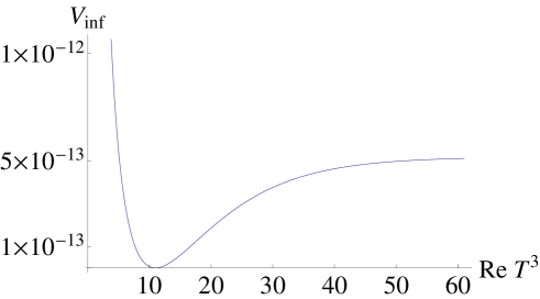
Figure 1: Inflaton potential $V_{\rm inf}$ on the ${\rm Im}\,T^{1}=0$ hypersurface.

As a result, it is found that the power spectrum of scalar curvature perturbation, its spectral index and tensor-to-scalar ratio are consistent with the current cosmological data,

$$P_{\xi}(k)\simeq 2.2\times 10^{-9},\,\,\,n_{s}\simeq 0.96,\,\,\,r\simeq 10^{-5},$$ (35)

with the enough $e$-foldings $N\simeq 58$ and then the parameters are chosen as,

$$J_{0}^{(3)}=\frac{1}{4000},\,\,J_{L}^{(3)}=\frac{3}{4000},\,\,c_{3}^{(3)}=\frac{1}{10}.$$ (36)

The running of the scalar spectral index is negligible, relative to the current observational sensitivity.

When the numerical values of the parameters are chosen as those in Eqs. (28), (29) and (36), the moduli VEVs become

$$(\text{Re}\langle T^{1}\rangle,\text{Re}\langle T^{2}\rangle,\text{Re}\langle T^{3}\rangle)\simeq(110,\;110,\;11),$$ (37)

in the unit $M_{\rm Pl}=1$. According to these moduli VEVs, the typical Kaluza-Klein mass scale is found as

$$M_{c}=\frac{\pi}{L}\simeq\frac{\pi}{\langle{\cal N}^{1/2}\rangle}\simeq 2.1\times 10^{16}\text{GeV},$$ (38)

which is close to the GUT scale due to the mild large volume of the fifth dimension, $\langle{\cal N}^{1/2}\rangle\simeq 364$. The mass of moduli $T^{I^{\prime}}$ and stabilizer fields $H_{i}$ are also given by

$$m_{T^{1}}\simeq m_{T^{2}}\simeq m_{H_{1}}\simeq m_{H_{2}}\simeq 4.8\times 10^{15}\,{\rm GeV},\,\,\,m_{T^{3}}\simeq m_{H_{3}}\simeq 4\times 10^{12}\,{\rm GeV},$$ (39)

and their F-terms become

$$F^{T^{1}}\simeq F^{T^{2}}\simeq F^{H_{1}}\simeq F^{H_{2}}\simeq 1\times 10^{-42},F^{T^{3}}\simeq F^{H_{3}}\simeq 1.6\times 10^{-36},$$ (40)

in the unit $M_{\rm Pl}=1$.

So far, we have specified the parameters relevant for the moduli and stabilizer fields. The parameters in the Kähler and superpotential (18) for the SUSY-breaking sector are considered as

$$\nu\simeq-1.567\cdots\times 10^{-14},\,\,w=-6\times 10^{-14},\,\,\Lambda=10^{-4},c_{X}^{(1)}=\frac{3}{10},\,\,c_{X}^{(2)}=\frac{1}{10},\,\,c_{X}^{(3)}=0,$$ (41)

where $\nu$ is proper chosen as realizing the Minkowski minimum. Then, the mass of the gravitino and the mass and F-term of $X$ are obtained as

$$m_{3/2}\simeq 395\,{\rm GeV},\,\,\,m_{X}\simeq 6\times 10^{8}\,{\rm GeV},\,\,\,\frac{F^{X}}{M_{\rm Pl}}\simeq 4541\,{\rm GeV},$$ (42)

which implies that the gravitino mass is suppressed by the Kähler metric of the SUSY-breaking field, $K_{X\bar{X}}\simeq 1/(c_{X}\cdot{\rm Re}T)\simeq 0.023$ as discussed in Sec. 3.2 and the concrete sparticle spectra are shown in Sec. 4.3.

3.5 Moduli-induced gravitino problem and reheating temperature

As mentioned in Sec. 3.3, the moduli and stabilizer fields are so heavy that they decay into the particles in the MSSM before the BBN. However, even if they are much heavier than O($100$ TeV), it has to be taken into account of the cosmological problem, e.g., the moduli-induced gravitino problem [38, 39].

The moduli decay width into the gravitino pair can be evaluated by the couplings between moduli and gravitinos in the unitary gauge,

$${\cal L}_{3/2}=\epsilon^{\mu\nu\rho\sigma}{\bar{\psi}}_{\mu}{\bar{\sigma}}_{\nu}\tilde{D}_{\rho}\psi_{\sigma}-e^{K/2}W^{\ast}\psi_{\mu}\sigma^{\mu\nu}\psi_{\nu}-e^{K/2}W{\bar{\psi}}_{\mu}{\bar{\sigma}}^{\mu\nu}{\bar{\psi}}_{\nu},$$ (43)

where $\psi_{\mu}$ denotes the gravitino in two-component formalism and the relevant covariant derivatives of the gravitino are $\tilde{D}_{\rho}\psi_{\sigma}=\partial_{\rho}\psi_{\sigma}+\frac{1}{4}(K_{J}\partial_{\rho}\phi^{J}-K_{\bar{J}}\partial_{\rho}{\bar{\phi}}^{{\bar{J}}})$. After carrying out a field-dependent chiral transformation,

$$\psi_{\mu}\rightarrow\left(\cfrac{W}{{\overline{W}}}\right)^{-1/4}\psi_{\mu},$$ (44)

the Lagrangian (43) is simplified as

$${\cal L}_{3/2} =\epsilon^{\mu\nu\rho\sigma}{\bar{\psi}}_{\mu}{\bar{\sigma}}_{\nu}\partial_{\rho}\psi_{\sigma}+\cfrac{\epsilon^{\mu\nu\rho\sigma}}{4}(G_{J}\partial_{\rho}\phi^{J}-G_{\bar{J}}\partial_{\rho}{\bar{\phi}}^{\bar{J}}){\bar{\psi}}_{\mu}{\bar{\sigma}}_{\nu}\psi_{\sigma}-e^{G/2}(\psi_{\mu}\sigma^{\mu\nu}\psi_{\nu}+{\bar{\psi}}_{\mu}{\bar{\sigma}}^{\mu\nu}{\bar{\psi}}_{\nu}),$$ (45)

where $G=K+\text{ln}|W|^{2}$ and $G_{J}=\partial_{J}G$. When we expand the moduli $T^{I^{\prime}}$ around the vacuum given by employing the reference point method (16) and (23), the Lagrangian (43) reduces to

$${\cal L}_{3/2} =-\cfrac{\epsilon^{\mu\nu\rho\sigma}}{2}{\bar{\Psi}}_{\mu}\gamma_{5}\gamma_{\nu}\partial_{\rho}\Psi_{\sigma}+\cfrac{\epsilon^{\mu\nu\rho\sigma}}{8}(\langle G_{T^{J^{\prime}}}\rangle\partial_{\rho}\delta T^{J^{\prime}}-\langle G_{\overline{T}^{J^{\prime}}}\rangle\partial_{\rho}\delta\overline{T}^{{\bar{J}}^{\prime}}){\bar{\Psi}}_{\mu}\gamma_{\nu}\Psi_{\sigma}$$

$$\hskip 13.0pt-\cfrac{1}{4}\langle e^{G/2}\rangle{\bar{\Psi}}_{\mu}[\gamma^{\mu},\gamma^{\nu}]\Psi_{\nu}-\cfrac{1}{8}\langle e^{G/2}\rangle(\langle G_{T^{J^{\prime}}}\rangle\delta T^{J^{\prime}}+\langle G_{{\overline{T}}^{{\bar{J}}^{\prime}}}\rangle\delta\overline{T}^{{\bar{J}}^{\prime}}){\bar{\Psi}}_{\mu}[\gamma^{\mu},\gamma^{\nu}]\Psi_{\nu},$$ (46)

in the four-component formalism of the gravitino $\Psi_{\mu}$. As shown in Eq. (39), the moduli and stabilizer fields, except for the pair ($T^{3},H_{3}$), are decoupled from the inflaton dynamics due to their heavy masses. Therefore, their decays can be neglected and do not give the sizable effects in the thermal history of the universe. In this respect, we focus on the decay processes of $T^{3}$, $H_{3}$, and SUSY-breaking field $X$.

3.5.1 The inflaton decay

First, we concentrate on the inflaton decay into gravitino pair. Since the gravitino wavefunction is described in terms of helicity $\pm 1/2$ components of the gravitino at a high-energy limit by the equivalence theorem, the inflaton decay width into the gravitino pair is estimated as

$$\Gamma(\sigma^{3}\rightarrow\Psi_{3/2}\Psi_{3/2}) \simeq\frac{1}{288\pi\langle K_{T^{3}\bar{T}^{3}}\rangle}\left|\left\langle\frac{D_{T^{3}}W}{W}\right\rangle\right|^{2}\cfrac{m_{T^{3}}^{5}}{m_{3/2}^{2}M_{\rm Pl}^{2}}\simeq\frac{1}{288\pi\langle K_{T^{3}\bar{T}^{3}}{\cal N}\rangle}\cfrac{m_{T^{3}}m_{3/2}^{2}}{M_{\rm Pl}^{2}}$$

$$\simeq 1.6\times 10^{-18}\;\;\text{GeV},$$ (47)

by employing the F-term of modulus (24) and numerical values of the mass, F-term of inflaton, and gravitino mass given by Eqs. (39) and (40). Here, the reduced Planck mass has been explicitly written. When the inflaton has the sizable F-term at the vacuum, the enhancement factor $m_{3/2}^{-2}$, as the longitudinal mode of the gravitino, induces the significant amount of gravitinos which would threaten to destroy the success of BBN. However, in our moduli inflation, this direct decay is so suppressed due to the almost vanishing F-term of the inflaton. Therefore, the dominant decay process of inflaton comes from the interactions with the gauge bosons,

$${\cal L}_{Tgg} =-\cfrac{1}{4(g_{a})^{2}}F^{a}_{\mu\nu}F^{a\mu\nu}-\cfrac{1}{4}\xi_{J^{\prime}}^{a}\delta T_{R}^{J^{\prime}}F^{a}_{\mu\nu}F^{a\mu\nu}-\cfrac{1}{8}\xi_{J^{\prime}}^{a}\delta T_{I}^{J^{\prime}}\epsilon^{\mu\nu\rho\sigma}F^{a}_{\mu\nu}F^{a}_{\rho\sigma},$$ (48)

where $T_{R}^{J^{\prime}}={\rm Re}\,T^{J^{\prime}}$, $T_{I}^{J^{\prime}}={\rm Im}\,T^{J^{\prime}}$. Now, the gauge kinetic functions $f_{a}(X,T)$ are considered as in Eq. (5). In general, $\xi_{X}^{a}X$ in the gauge kinetic function (5) could appear, because the R-symmetry is explicitly broken by the constant superpotential $w$ in Eq. (18).

The inflaton decay width into the gauge bosons are

$$\sum_{a=1}^{3}\Gamma(\sigma^{3}\rightarrow g^{(a)}g^{(a)}) \simeq\sum_{a=1}^{3}\cfrac{N_{G}^{a}}{128\pi}\left\langle\cfrac{\xi_{3}^{a}}{\sqrt{2K_{T^{3}\bar{T}^{3}}}}\right\rangle^{2}\cfrac{m_{T^{3}}^{3}}{M_{\rm Pl}^{2}}\simeq 3.95\,\,\,{\rm GeV},$$ (49)

with the numerical values of mass and VEV of modulus (37), (39), where $N_{G}^{a}$ are the number of the gauge bosons for the gauge groups $U(1)_{Y}$, $SU(2)_{L}$, $SU(3)_{C}$ and the nonvanishing coefficients in the gauge kinetic function are chosen as $\xi_{3}^{1}=\xi_{3}^{2}=\xi_{3}^{3}=0.22$ to realize the gauge coupling unification at the GUT scale $M_{\rm GUT}\simeq 2\times 10^{16}\,{\rm GeV}$. Although there are the other decay processes via the inflaton decay into the gauginos $\lambda^{a}$ given by the interactions,

$${\cal L}_{T\lambda\lambda} =-\cfrac{i}{2}\sum_{a}{\rm Re}\,f_{a}(\lambda^{a}\sigma^{\mu}D_{\mu}\bar{\lambda^{a}}+({\rm H.c.}))+\cfrac{i}{2}\sum_{a}{\rm Im}\,f_{a}D_{\mu}(\lambda^{a}\sigma^{\mu}\bar{\lambda^{a}})$$

$$\hskip 13.0pt+\sum_{a}\left(\cfrac{1}{4}\frac{\partial f_{a}}{\partial T^{I^{\prime}}}F^{T^{I^{\prime}}}\lambda^{a}\lambda^{a}+({\rm H.c.})\right),$$ (50)

where $D_{\mu}$ is the covariant derivative for gaugino, such decay channels are suppressed by the small masses of gauginos and almost vanishing F-term of inflaton such as

$$\sum_{a=1}^{3}\Gamma(\sigma^{3}\rightarrow\tilde{\lambda^{a}}\tilde{\lambda^{a}})\simeq\sum_{a=1}^{3}\frac{m_{T^{3}}}{16\pi}\frac{(\xi_{3}^{a})^{2}m_{\lambda^{a}}^{2}}{M_{\rm Pl}^{2}}\simeq 1.5\times 10^{-21}\,\text{GeV},$$ (51)

with $m_{\lambda^{3}}\simeq 1.5\,{\rm TeV}$ and the derivative of F-term for the inflaton,

$$\left\langle\frac{\partial F^{T^{3}}}{\partial T^{3}}\right\rangle=\left\langle\frac{\partial}{\partial T^{3}}e^{K/2}\left(K^{T^{3}\bar{T}^{3}}|D_{T^{3}}W|^{2}+K^{T^{3}\bar{H}^{3}}D_{T^{3}}W\overline{D_{H^{3}}W}\right)\right\rangle\sim O\left(\frac{m_{3/2}^{4}}{m_{T^{3}}^{2}}\right).$$ (52)

The decays from the inflaton into sfermions are also suppressed because of the factor, $m_{\text{sfermion}}/m_{T^{3}}$, if the masses of sfermions are of O($1$ TeV). Other decays from the inflaton into the fermion pairs and quark-quark-gluon are negligible due to their small masses and phase factors, respectively, as pointed out in Ref. [39]. The $\mu$-term does not give the sizable effects for the inflaton decay process, because we consider the tiny $\mu$-term ($\sim$ $500$ GeV) in the light of naturalness as shown in Sec. 4.1. Finally, we comment on a single gravitino production via the inflaton decay into the modulino and gravitino. Since the mixing terms between $T^{3}$ and $H_{3}$ in the mass squared matrices are controlled by the SUSY-breaking scale, i.e., the gravitino mass, the mass difference between the inflaton and modulino as its superpartner is of the order of the gravitino mass. Therefore, the inflaton decay width into the modulino $\tilde{\sigma}^{3}$ and gravitino is suppressed by the phase factor $m_{3/2}/m_{T^{3}}$,

$$\Gamma(\sigma^{3}\rightarrow{\tilde{\sigma}^{3}}\Psi_{\text{3/2}}) \simeq\frac{1}{48\pi}\left(\frac{m_{T^{3}}}{M_{\rm Pl}}\right)^{2}\left(\frac{m_{3/2}}{m_{T^{3}}}\right)m_{3/2}\simeq 7.2\times 10^{-22}\,\text{GeV},$$ (53)

with $m_{3/2}=395\,{\rm GeV}$, $m_{T^{3}}=4\times 10^{12}\,{\rm GeV}$ given by Eqs. (39) and (42). The inflaton decay into the SUSY-breaking field $X$ is also suppressed, because there is no tree-level interaction between $X$ and $T^{3}$ due to the vanishing $U(1)_{3}$ charge of $X$. As a result, the branching ratios of the moduli decaying into the gravitino(s) are summarized as

$$\Gamma_{\text{all}}^{\sigma^{3}}\equiv\Gamma(\sigma^{3}\rightarrow\text{all})\simeq\sum_{a=1}^{3}\Gamma(\sigma^{3}\rightarrow g^{(a)}g^{(a)})\simeq 3.95\,\,\,{\rm GeV},$$

$$\text{Br}(\sigma^{3}\rightarrow\Psi_{\text{3/2}}\Psi_{\text{3/2}})\simeq\frac{\Gamma(\sigma^{3}\rightarrow\Psi_{\text{3/2}}\Psi_{\text{3/2}})}{\Gamma_{\text{all}}^{\sigma^{3}}}\simeq 1.4\times 10^{-20},$$

$$\text{Br}(\sigma^{3}\rightarrow\tilde{\sigma}^{3}\Psi_{\text{3/2}})\simeq\frac{\Gamma(\sigma^{3}\rightarrow\tilde{\sigma}^{3}\Psi_{\text{3/2}})}{\Gamma_{\text{all}}^{\sigma^{3}}}\simeq 1.8\times 10^{-22},$$ (54)

and then the reheating temperature is roughly estimated by equaling the expansion rate of the Universe to the total decay width of inflaton,

$$\Gamma_{\rm all}^{\sigma^{3}}=H_{R}\Leftrightarrow T_{R}=\left(\cfrac{\pi^{2}g_{\ast}}{90}\right)^{-1/4}\sqrt{\Gamma_{\rm all}M_{\rm Pl}}\simeq 1.38\times 10^{9}~{}{\rm GeV},$$ (55)

where $H_{R}=H(T_{R})$ and $g_{\ast}(T_{R})=915/4$ is the effective degrees of freedom of the radiation in the MSSM at the reheating. The gravitino yield $Y_{3/2}$ via the inflaton decay is suppressed due to the tiny branching ratio of the inflaton decay into the gravitino(s),

$$Y_{3/2}=\frac{n_{3/2}}{s}\simeq\text{Br}(\sigma^{3}\rightarrow\tilde{\sigma}^{3}\Psi_{\text{3/2}})\frac{3T_{R}}{4m_{T^{3}}}\simeq 3.8\times 10^{-24},$$ (56)

with $m_{3/2}=395\,{\rm GeV}$, $T_{R}=1.38\times 10^{9}\,{\rm GeV}$ $s=4\rho/3T$, where $n_{3/2}$, $s$, and $\rho$ are the number density of the gravitino, entropy, and energy density of the Universe, respectively. Now it is supposed that the coherent oscillation of the inflaton field dominates the energy density of the Universe after the inflation and there is no entropy production after the inflation as shown later.

It is remarkable that the supersymmetric moduli stabilization is important to suppress the direct decays from the inflaton into the gravitino(s) which give the solution to the cosmological moduli problem, especially the moduli-induced gravitino problem. The other gravitino production from the stabilizer fields, the SUSY-breaking field, and the thermal bath can be estimated in the next section.

3.5.2 The decay of stabilizer and SUSY-breaking fields

The stabilizer field $H_{3}$ is stabilized at the origin during the inflation and after that, Re $H_{3}$ oscillates around its vacuum (23) deviated from the supersymmetric one (16). On the other hand, Im $H_{3}$ and Im $X$ evolve to the origin during inflation and do not oscillate after the inflation as shown in Appendices. A and B. Similarly, the SUSY-breaking field Re $X$ oscillates around its vacuum after the inflation. From the analyses in Appendices. A and B, the amplitudes of both fields are found as

$$\Delta h_{3}\simeq\frac{m_{3/2}}{m_{H_{3}}},\,\,\,\,\,\Delta x\simeq\left(\frac{m_{3/2}}{m_{X}}\right)^{2},$$ (57)

with $h_{3}={\rm Re}\,H_{3}$ and $x={\rm Re}\,X$. By comparing their masses given in Eq. (39) with the reheating temperature (55), the coherent oscillations of both fields $h_{3}$ and $x$ start before the reheating process. When $H_{3}$ does not couple to the fields in the MSSM, the dominant decay process is

$$\Gamma_{\rm all}^{h_{3}}\equiv\Gamma(h_{3}\rightarrow\Psi_{3/2}\Psi_{3/2}) \simeq\frac{1}{288\pi K_{H_{3}\bar{H}_{3}}}\left|\left\langle\frac{D_{H_{3}}W}{W}\right\rangle\right|^{2}\cfrac{m_{H_{3}}^{5}}{m_{3/2}^{2}M_{Pl.}^{2}}\simeq\frac{1}{288\pi\langle K_{H_{3}\bar{H}_{3}}{\cal N}\rangle}\cfrac{m_{H_{3}}^{3}}{M_{\rm Pl}^{2}}$$

$$\simeq 0.02\;\;\text{GeV},$$ (58)

which implies the decay time of $h_{3}$ is smaller than the time of the coherent oscillation of $h_{3}$ and reheating, that is, $H^{h_{3}}_{\rm osc}>H(T_{R})>H^{h_{3}}_{\rm dec}$, with $H^{h_{3}}_{\rm osc}\simeq m_{h_{3}}$ and $H^{h_{3}}_{\rm dec}\simeq\Gamma(h_{3}\rightarrow\Psi_{3/2}\Psi_{3/2})$. Here and in what follows, $H_{\rm R}$, $H_{\rm osc}^{\Phi}$, and $H_{\rm dec}^{\Phi}$ refer to the Hubble parameters at the time of reheating, beginning of oscillation of relevant fields $\Phi$, and decay of $\Phi$. The scale factors of $4$D spacetime $a_{R}$, $a_{\rm osc}^{\Phi}$, and $a_{\rm dec}^{\Phi}$ are also defined in the same way as the Hubble parameters, $H_{\rm R}$, $H_{\rm osc}^{\Phi}$, and $H_{\rm dec}^{\Phi}$. The energy density of coherent oscillation $h_{3}$ is

$$\rho_{h_{3}}\simeq\frac{1}{2}m_{H_{3}}^{2}(\Delta h_{3})^{2}\simeq\frac{1}{2}m_{3/2}^{2}\left(\frac{a}{a^{h_{3}}_{\rm osc}}\right)^{-3},$$ (59)

where $a^{h_{3}}_{\rm osc}$ stands for the scale factor at the time when $h_{3}$ begins to oscillate and $\rho_{h_{3}}$ is converted into the gravitino yield hereafter,

$$Y_{3/2}^{h_{3}}=\frac{2\rho_{h_{3}}}{m_{H_{3}}s}\simeq\frac{1}{4}\frac{m_{3/2}^{2}T_{R}}{m_{H_{3}}^{3}}\simeq 8.2\times 10^{-25},$$ (60)

with $m_{3/2}=395\,{\rm GeV}$, $T_{R}=1.38\times 10^{9}\,{\rm GeV}$, and $m_{H_{3}}=4\times 10^{12}\,{\rm GeV}$. Here we employed that the entropy production from $h_{3}$ can be neglected. In our model, the following inequality is satisfied due to the tiny mass of the gravitino and then $h_{3}$ does not dominate the Universe and release the significant entropy,

$$1\gg\frac{\rho_{h_{3}}}{\rho_{R}}\biggl{|}_{T=T_{\rm dec}^{h_{3}}}=\frac{\rho_{h_{3}}}{\rho}\biggl{|}_{\rm end}\left(\frac{T_{R}}{T_{t_{\rm dec}^{h_{3}}}}\right)\simeq\frac{m_{3/2}^{2}M_{\rm Pl}^{2}}{2V_{\rm inf}}\left(\frac{T_{R}}{T_{t_{\rm dec}^{h_{3}}}}\right),$$ (61)

where $\rho_{h_{3}}$, $\rho_{R}$ are the energy densities of $h_{3}$ and radiation, respectively. $\rho|_{\rm end}=V_{\rm inf}\simeq{\cal O}(10^{-13})$ denotes the energy density at the end of inflation and $T_{\rm dec}^{h_{3}}$ is the decay temperature of $h_{3}$,

$$T_{\rm dec}^{h_{3}}=\left(\cfrac{\pi^{2}g_{\ast}}{90}\right)^{-1/4}\sqrt{\Gamma_{\rm all}^{h_{3}}M_{\rm Pl}}\simeq 8.6\times 10^{7}~{}{\rm GeV}.$$ (62)

Furthermore, the SUSY-breaking field also produces the gravitinos through the following dominant decay channel:

$$\Gamma(x\rightarrow\Psi_{3/2}\Psi_{3/2}) \simeq\frac{1}{288\pi\langle K_{X\bar{X}}\rangle}\left|\left\langle\frac{D_{X}W}{W}\right\rangle\right|^{2}\cfrac{m_{X}^{5}}{m_{3/2}^{2}M_{\rm Pl}^{2}}\simeq\frac{1}{288\pi\langle K_{X\bar{X}}\rangle}\left|\frac{\nu}{w}\right|^{2}\cfrac{m_{X}^{5}}{m_{3/2}^{2}M_{\rm Pl}^{2}}.$$ (63)

With the parameters (41), the VEVs of moduli (37), and mass of $\Psi_{3/2}$ and $X$ (42), the total decay width of $X$ then becomes

$$\Gamma_{\rm all}^{x}\equiv\Gamma(x\rightarrow\Psi_{3/2}\Psi_{3/2})\simeq 3.7\times 10^{8}\;\;\text{GeV}.$$ (64)

Therefore, the decay time of $x$ is smaller than that of reheating, that is, $H^{x}_{\rm osc}>H^{x}_{\rm dec}\gg H(T_{R})$, with $H^{x}_{\rm osc}\simeq m_{X}$ and $H^{x}_{\rm dec}\simeq\Gamma(x\rightarrow\Psi_{3/2}\Psi_{3/2})$. The energy density of the coherent oscillation $x$ is converted into that of the gravitino as

$$\rho_{x}\simeq\frac{1}{2}m_{x}^{2}(\Delta x)^{2}\simeq\frac{1}{2}\left(\frac{m_{3/2}^{4}}{m_{x}^{2}}\right)\left(\frac{a^{x}_{\rm dec}}{a^{x}_{\rm osc}}\right)^{-3}\left(\frac{a_{R}}{a^{x}_{\rm dec}}\right)^{-4},$$ (65)

at the time of reheating, where the gravitino is relativistic at the time of production. By employing the scale factors,

$$\frac{a_{R}}{a_{\rm osc}^{\sigma^{3}}}=\left(\frac{\sqrt{6}\Gamma_{\rm all}^{\sigma^{3}}}{m_{T^{3}}}\right)^{-2/3},\,\,\,\frac{a_{\rm osc}^{x}}{a_{\rm osc}^{\sigma^{3}}}=\left(\frac{\sqrt{6}m_{X}}{m_{T^{3}}}\right)^{-2/3},\,\,\,\frac{a_{\rm dec}^{x}}{a_{\rm osc}^{\sigma^{3}}}=\left(\frac{6(\Gamma_{\rm all}^{x}\,m_{X})^{2}}{m_{3/2}^{4}}\right)^{-1/3},$$ (66)

the gravitino yield is

$$Y_{3/2}^{x}=\frac{2\rho_{x}}{m_{x}s}\simeq\frac{3}{2}\frac{T_{R}}{m_{X}}\left(\frac{m_{3/2}}{m_{X}}\right)^{16/3}\left(\frac{\Gamma_{\rm all}^{\sigma^{3}}}{\Gamma_{\rm all}^{x}}\right)^{2/3}\simeq 2\times 10^{-32},$$ (67)

with the numerical values given by Eqs. (42), (54), (55), and (64). It is found that the gravitino production via $x$ decay is suppressed by the tiny mass of the gravitino and it is not the dominant source for the relic abundance of the gravitino. The entropy production from $x$ can be also neglected in the same way as that of $h_{3}$. As pointed out in Ref. [40], under $m_{3/2}\ll m_{\rm X}\ll m_{T^{3}}\leq\Lambda$, the gravitino production is significantly relaxed and this condition is satisfied in our model. Note that when $\Lambda$ is smaller than the inflaton mass, we have to take account of the inflaton decay into the fields in the hidden sector.

4 Gravitino dark matter and the Higgs boson mass

4.1 Yukawa couplings and naturalness

Before estimating the relic abundance of the gravitino, we specify the Yukawa couplings and $\mu$-term in the superpotential which can be only introduced at the orbifold fixed points $y=0,L$, where the SUSY is reduced to $4$D ${\cal N}=1$. As stated in Sec. 3.1, we consider the Yukawa interactions in the MSSM at the orbifold fixed point $y=0$,

$$W_{\rm Yukawa}=\lambda_{ij}^{u}{\cal Q}_{i}{\cal H}_{u}{\cal U}_{j}+\lambda_{ij}^{d}{\cal Q}_{i}{\cal H}_{d}{\cal D}_{j}+\lambda_{ij}^{e}{\cal L}_{i}{\cal H}_{d}{\cal E}_{j}+\lambda_{ij}^{n}{\cal L}_{i}{\cal H}_{u}N_{j},$$ (68)

where $\lambda_{ij}^{u,d,e,n}$ are the holomorphic Yukawa coupling constants and are supposed to be of ${\cal O}(1)$. After the canonical normalization of fields in the MSSM, the physical Yukawa couplings are expressed as

$$y_{ij}^{u} =\frac{\lambda_{ij}^{u}}{\sqrt{\langle Y_{{\cal Q}_{i}}Y_{{\cal H}_{u}}Y_{{\cal U}_{j}}\rangle}},\;\;\;\;y_{ij}^{d}=\frac{\lambda_{ij}^{d}}{\sqrt{\langle Y_{{\cal Q}_{i}}Y_{{\cal H}_{d}}Y_{{\cal D}_{j}}\rangle}},\;\;\;\;y_{ij}^{e}=\frac{\lambda_{ij}^{e}}{\sqrt{\langle Y_{{\cal L}_{i}}Y_{{\cal H}_{d}}Y_{{\cal E}_{j}}\rangle}},\;\;\;\;y_{ij}^{n}=\frac{\lambda_{ij}^{n}}{\sqrt{\langle Y_{{\cal L}_{i}}Y_{{\cal H}_{u}}Y_{{\cal N}_{j}}\rangle}},$$

where

$$Y_{a}\equiv 2{\cal N}^{1/3}({\rm Re}T)\left\{Y(c_{a}\cdot T)+\tilde{\Omega}^{(4)}_{a,X}({\rm Re}T)|X|^{2}+{\cal O}(|X|^{4})\right\}$$ (70)

The function $Y(z)$ is always positive, and approximated as

$$Y(z)\equiv\frac{1-e^{-2{\rm Re}z}}{2{\rm Re}z}\simeq\begin{cases}\frac{1}{2\text{Re}z},&\text{Re}z>0\\ \frac{1}{2|\text{Re}z|}\text{exp}(2|\text{Re}z|).&\text{Re}z<0.\end{cases}$$ (71)

In the 5D viewpoint, the wavefunctions of fields are localized toward $y=0$ ($y=L$) in the case that $c_{a}\cdot\langle\text{Re}T\rangle$ is positive (negative). As can be seen in Eq. (71), $y_{ij}^{u,d,e,n}$ are of ${\cal O}(1)$ or exponentially small when all the relevant fields are localized toward $y=0$ or $y=L$, respectively.

Therefore, we expect that the mass hierarchies of elementary particles and the extreme smallness of the neutrino masses can be realized even in the case of Dirac neutrinos. In fact, when we choose the $U(1)_{I^{\prime}}$ charges and ${\cal O}(1)$ values of the holomorphic Yukawa couplings $\lambda^{u,d,e,n}_{i,j}$ in Tables 1 and 2, the observed masses and mixing angles of quarks and leptons at the electroweak scale can be realized. Here, we employ the full one-loop RG equations of the MSSM from the GUT to the EW scale. It is remarkable that the flavor structure of soft SUSY-breaking terms is determined by the $U(1)_{I^{\prime}}$ charge assignment as can be seen in the Kähler potential (LABEL:eq:effKahler). In fact, the soft SUSY-breaking terms at the GUT scale are determined by the following formula [41, 42]:

$$M_{a} =\langle F^{I}\partial_{I}\text{ln}\left(\text{Re}f^{a}\right)\rangle,$$

$$m_{Q_{\alpha}}^{2} =-\langle F^{I}\bar{F}^{\bar{J}}\partial_{I}\partial_{\bar{J}}\text{ln}Y_{Q_{\alpha}}\rangle,$$

$$A_{ij}^{u} =\langle F^{I}\partial_{I}\text{ln}\left(Y_{{\cal H}_{u}}Y_{{\cal Q}_{i}}Y_{{\cal U}_{j}}\right)\rangle,$$

$$A_{ij}^{d} =\langle F^{I}\partial_{I}\text{ln}\left(Y_{{\cal H}_{d}}Y_{{\cal Q}_{i}}Y_{{\cal D}_{j}}\right)\rangle,$$

$$A_{ij}^{e} =\langle F^{I}\partial_{I}\text{ln}\left(Y_{{\cal H}_{d}}Y_{{\cal L}_{i}}Y_{{\cal E}_{j}}\right)\rangle,$$

$$A_{ij}^{n} =\langle F^{I}\partial_{I}\text{ln}\left(Y_{{\cal H}_{u}}Y_{{\cal L}_{i}}Y_{{\cal N}_{j}}\right)\rangle,$$ (72)

where indices $I$ and $J$ run over all the chiral multiplets. Then, the $U(1)_{I^{\prime}}$ charge assignment in Table 1 and the F-term of the SUSY-breaking field $X$ given by Eq. (42) give rise to the soft scalar masses and gluino mass in Table 3. By contrast, the A-terms are almost vanishing due to the tiny F-terms of moduli. Here and hereafter, we parametrize the ratios of gaugino masses at the GUT scale as

$$r_{1}=\frac{M_{1}(M_{\rm GUT})}{M_{3}(M_{\rm GUT})},\,\,\,r_{2}=\frac{M_{2}(M_{\rm GUT})}{M_{3}(M_{\rm GUT})},$$ (73)

where $M_{1}(M_{\rm GUT})$, $M_{2}(M_{\rm GUT})$, and $M_{3}(M_{\rm GUT})$ are the bino, wino, and gluino masses at the GUT scale, $M_{\rm GUT}\simeq 2\times 10^{16}\,{\rm GeV}$. The ratios of gaugino masses are controlled by the parameters $\xi_{X}^{a}$ in the gauge kinetic function (5) without spoiling the gauge coupling unification due to the tiny VEV of $X$.

$c_{{\cal Q}_{i}}^{I^{\prime}=1}=(0.1,~{}0.1,~{}1.1)$	$c_{{\cal L}_{i}}^{I^{\prime}=1}=(0.1,~{}0.1,~{}1.6)$	$c_{{\cal H}_{u}}^{I^{\prime}=1}=0$
$c_{{\cal Q}_{i}}^{I^{\prime}=2}=(-0.1,-0.1,0.8)$	$c_{{\cal L}_{i}}^{I^{\prime}=2}=(-0.1,-0.1,~{}0)$	$c_{{\cal H}_{u}}^{I^{\prime}=2}=0.1$
$c_{{\cal Q}_{i}}^{I^{\prime}=3}=(0.1,~{}0.4,~{}1)$	$c_{{\cal L}_{i}}^{I^{\prime}=3}=(0.1,~{}0.5,~{}0)$	$c_{{\cal H}_{u}}^{I^{\prime}=3}=-0.9$
$c_{{\cal U}_{i}}^{I^{\prime}=1}=(0.1,~{}0.1,~{}0.6)$	$c_{{\cal E}_{i}}^{I^{\prime}=1}=(0.1,~{}0.2,~{}0.2)$	$c_{{\cal H}_{d}}^{I^{\prime}=1}=0$
$c_{{\cal U}_{i}}^{I^{\prime}=2}=(-0.1,-0.1,0.3)$	$c_{{\cal E}_{i}}^{I^{\prime}=2}=(-0.1,-0.1,0)$	$c_{{\cal H}_{d}}^{I^{\prime}=2}=0$
$c_{{\cal U}_{i}}^{I^{\prime}=3}=(-0.2,~{}0.2,~{}1)$	$c_{{\cal E}_{i}}^{I^{\prime}=3}=(-0.2,~{}0,~{}-0.5)$	$c_{{\cal H}_{d}}^{I^{\prime}=3}=-0.1$
$c_{{\cal D}_{i}}^{I^{\prime}=1}=(0.1,~{}0.1,~{}0.2)$	$c_{N_{i}}^{I^{\prime}=1}=(0.1,~{}0.1,~{}0.1)$
$c_{{\cal D}_{i}}^{I^{\prime}=2}=(-0.1,-0.1,0)$	$c_{N_{i}}^{I^{\prime}=2}=(-0.3,-0.3,-0.3)$
$c_{{\cal D}_{i}}^{I^{\prime}=3}=(0.3,~{}0.2,~{}-0.5)$	$c_{N_{i}}^{I^{\prime}=3}=(-0.7,~{}-0.7,~{}-0.7)$

Table 1: $U(1)_{I^{\prime}}$ flavor charges of the quarks, leptons, and Higgs.

$|\lambda^{u}_{ij}|$	$|\lambda^{d}_{ij}|$
$\displaystyle\left(\begin{array}[]{ccc}0.32&0.35&0.95\\ 0.22&0.42&0.33\\ 0.51&0.48&1.5\end{array}\right)$ (77)	$\displaystyle\left(\begin{array}[]{ccc}0.45&0.5&0.59\\ 0.28&0.24&0.38\\ 1.03&1.02&0.81\end{array}\right)$ (81)
$|\lambda^{e}_{ij}|$	$|\lambda^{n}_{ij}|$
$\displaystyle\left(\begin{array}[]{ccc}0.28&0.22&0.52\\ 0.4&1.15&0.31\\ 0.8&1.02&1.05\end{array}\right)$ (85)	$\displaystyle\left(\begin{array}[]{ccc}0.77&0.85&0.69\\ 0.25&0.98&0.58\\ 0.34&0.26&1.03\end{array}\right)$ (89)

Table 2: ${\cal O}(1)$ values of the holomorphic Yukawa couplings $\lambda^{u,d,e,n}_{ij}$ in the superpotential (68).

Sparticles	Mass[GeV]	(S)Particles	Mass[GeV]
$m_{\tilde{{\cal Q}}_{1}}$	1682	$m_{\tilde{{\cal L}}_{3}}$	2834
$m_{\tilde{{\cal Q}}_{2}}$	1530	$m_{\tilde{{\cal E}}_{1}}$	1157
$m_{\tilde{{\cal Q}}_{3}}$	581	$m_{\tilde{{\cal E}}_{2}}$	2390
$m_{\tilde{{\cal U}}_{1}}$	1157	$m_{\tilde{{\cal E}}_{3}}$	2298
$m_{\tilde{{\cal U}}_{2}}$	1698	$m_{\tilde{N}_{1}}$	414.5
$m_{\tilde{{\cal U}}_{3}}$	799	$m_{\tilde{N}_{2}}$	414.5
$m_{\tilde{{\cal D}}_{1}}$	1636	$m_{\tilde{N}_{3}}$	414.5
$m_{\tilde{{\cal D}}_{2}}$	1698	$M_{{\cal H}_{u}}$	1100
$m_{\tilde{{\cal D}}_{3}}$	2298	$M_{{\cal H}_{d}}$	298.5
$m_{\tilde{{\cal L}}_{1}}$	1682	$M_{3}$	550
$m_{\tilde{{\cal L}}_{2}}$	1396

Table 3: The soft scalar masses $m_{\tilde{Q}_{\alpha}}$, the up- and down-type Higgs masses $M_{{\cal H}_{u,d}}$, and the gluino mass $M_{3}$ at the GUT scale. The subscripts $\tilde{Q}_{\alpha}$ denote the mass eigenvalues for the left-handed $\tilde{\cal Q}_{i}$, up-type right-handed $\tilde{\cal U}_{i}$, down-type right-handed $\tilde{\cal D}_{i}$ squarks, left-handed $\tilde{\cal L}_{i}$, right-handed $\tilde{\cal E}_{i}$ charged sleptons, and right-handed sneutrinos $\tilde{N}_{i}$ with the three-generation $i=1,2,3$.

On the other hand, the $\mu$-term can be generated by the following superpotential:

$$W_{\mu-{\rm term}}=\sum_{i=1}^{3}\kappa_{i}H_{i}{\cal H}_{u}{\cal H}_{d},$$ (90)

where $\kappa_{i}$ are the $O(1)$ dimensionless couplings, $H_{i}$ are the stabilizer fields with R-charge $2$, whereas Higgs chiral superfields do not have the R-charge. These cubic interactions do not affect the moduli stabilization as well as the moduli inflation due to the almost vanishing VEVs of the Higgs fields. Thus, it is possible to consider the VEVs of the stabilizer fields $H_{i}$ as the origin of the $\mu$-term. After the canonical normalization of the relevant fields, the $\mu$-term at the GUT scale becomes

$$\mu=\sum_{i=1}^{3}\frac{\kappa_{i}\langle H_{i}\rangle}{\langle Y_{H_{i}}Y_{{\cal H}_{u}}Y_{{\cal H}_{d}}\rangle}.$$ (91)

Especially, in the case of $\kappa_{2}=\kappa_{3}=0$, the scale of the $\mu$-term is chosen as TeV scale,

$$\mu\simeq 3.8\times 10^{-3}\frac{m_{3/2}}{m_{H_{1}}}M_{\rm Pl}\simeq{\cal O}(500\,{\rm GeV}),$$ (92)

where $\kappa_{1}=2/3$, $m_{3/2}=395\,{\rm GeV}$, $m_{H_{1}}\simeq 4.8\times 10^{15}\,{\rm GeV}$, and $\langle H_{1}\rangle\simeq m_{3/2}/m_{H_{1}}$ are given by Eq. (23) and the factor $3.8\times 10^{-3}$ comes from the mild large volume of the fifth dimension and normalization factors for $H_{1}$, ${\cal H}_{u}$, and ${\cal H}_{d}$. The EW symmetry breaking requires the following relation between the mass of the $Z$-boson, $m_{Z}$ and soft SUSY-breaking masses of the up-type Higgs $m_{{\cal H}_{u}}$:

$$\frac{m_{Z}^{2}}{2} \simeq-m_{H_{u}}^{2}(M_{\rm EW})-\left|\mu(M_{\rm EW})\right|^{2}+O\left(\frac{1}{{\rm tan^{2}}\beta}\right),$$ (93)

in the limit of large value of tan$\beta$, where $\mu(M_{\rm EW})$ and $m_{H_{u}}(M_{\rm EW})$ are the $\mu$-term and $m_{H_{u}}$ at the EW scale, respectively. The VEVs of up- and down-type Higgs fields are denoted by $v_{u}=v\,{\rm sin}\beta$ and $v_{d}=v\,{\rm cos}\beta$ with $v=174$  GeV. Thus, the observed $Z$-boson mass indicates $|\mu(M_{\rm EW})|\sim|m_{H_{u}}(M_{\rm EW})|\sim m_{Z}$; otherwise $\mu$ and $m_{H_{u}}$ have to be properly tuned to obtain the EW vacuum. We adopt the measure of the degree of tuning the $\mu$-term at the GUT scale as

$$\Delta_{\mu}=\frac{1}{2}\frac{\partial\ln m_{Z}^{2}}{\partial\ln|\mu|},$$ (94)

and then $100\times|\Delta_{\mu}^{-1}|$ % represents the degree of tuning to obtain the $Z$-boson mass $m_{Z}=91.2$ GeV [43]. Although the conventional CMSSM scenario requires more severe tuning than the degree of $0.1$ %, as pointed out in Ref. [2], certain ratios of the nonuniversal gaugino masses at the GUT scale relax the degree of tuning and observed 125 GeV Higgs boson mass at the same time.

4.2 Relic abundance of the gravitino

We are now ready to estimate the relic abundance of the gravitino. As stated in Sec. 3.5, there are no significant gravitino productions from the inflaton, moduli, stabilizer, and SUSY-breaking fields after the inflation. However, there are two processes to produce the gravitinos associated with the decay of other particles in the MSSM.

One of them is the decay from the thermal bath which is constituted of the relativistic particles after the reheating process. On the thermal bath, the dominant decay process comes from gauginos into gravitinos, because the couplings between the gravitino and other sparticles are more suppressed than those of gauginos as discussed in Refs. [44, 45]. The abundance of the gravitino is estimated as

$$\Omega_{3/2}^{TP}h^{2}=\sum_{a=1}^{3}\left(1+\cfrac{M_{a}(T_{R})^{2}}{3m_{3/2}^{2}}\right)w_{a}g_{a}(T_{R})^{2}~{}{\rm ln}\left(\cfrac{k_{a}}{g_{a}(T_{R})}\right)\left(\cfrac{m_{3/2}}{100\text{GeV}}\right)\left(\cfrac{T_{R}}{10^{10}{\rm GeV}}\right),$$ (95)

where $w_{a}$ and $k_{a}$ are the parameters whose values are defined in Ref. [45] and $h$ is a dimensionless Hubble parameter. The thermal production of the gravitino is drawn in Fig. 2 in terms of the ratios of gaugino masses at the GUT scale $M_{\rm GUT}$, $r_{1}=M_{1}(M_{\rm GUT})/M_{3}(M_{\rm GUT})$ and $r_{2}=M_{2}(M_{\rm GUT})/M_{3}(M_{\rm GUT})$ with $M_{3}(M_{\rm GUT})=550$ GeV. The gaugino masses at the reheating temperature $M_{a}(T_{R})$ can be expressed as $M_{a}(M_{\rm GUT})$ by employing the one-loop RG equations in the MSSM. The Planck Collaboration reported that the abundance of dark matter resides in the range of $0.1175\leq\Omega_{3/2}^{TP}h^{2}\leq 0.1219$ [22], where the upper and lower limits correspond to the dotted curves in Fig. 2. Here we assume that the dark matter only consists of the abundance of the thermally produced gravitino.

NNLSP(Higgsino-like neutralino)	Mass[GeV]
$\tilde{\chi}_{3}^{0}$	441
NLSPs(right-handed sneutrinos)	mass[GeV]
$\tilde{\nu}_{e_{2}}$	415
$\tilde{\nu}_{\mu_{2}}$	415
$\tilde{\nu}_{\tau_{2}}$	415
LSP(gravitino)	mass[GeV]
$\Psi_{3/2}$	395

Table 4: The masses of NNLSP, NLSPs, and the gravitino at the EW scale for the reference point $(r_{1},r_{2})=(6,3.5)$. The subscripts denote the mass eigenvalues for the sneutrinos ($\tilde{\nu}$), the Higgsino-like neutralino ($\tilde{\chi}$).

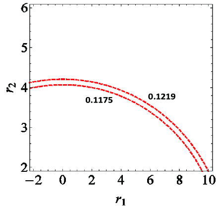
Figure 2: Contours of the thermal abundance of the gravitino in the ($r_{1},r_{2}$)-plane.

The other process is the nonthermal gravitino productions from the NLSP and/or next-to-next-to-lightest supersymmetric particle (NNLSP). As shown in Table 4, when we take the ratios of gaugino masses $(r_{1},r_{2})=(6,3.5)$ consistent with the observed relic abundance of dark matter in Fig. 2, the NLSPs and NNLSP correspond to the degenerated sneutrinos and Higgsino-like neutralino, respectively. The relevant sparticle spectra are obtained by employing the one-loop RG equations in the MSSM from GUT to EW scale with $(r_{1},r_{2})=(6,3.5)$ and the input parameters in Table 3. The full sparticle spectra are shown in the next section. Note that the degenerated sneutrinos do not have sizable interactions with the other (s)particles due to the tiny Yukawa couplings of Dirac-type neutrinos and then the soft SUSY-breaking masses of right-handed sneutrinos do not receive significant loop corrections.

Since the gravitino and right-handed sneutrinos are weakly coupled with the other (s)particles, they are not thermalized. Thus, the nonthermal gravitino productions from the higgsino-like neutralino and sneutrinos are roughly estimated as

$$\Omega_{3/2}^{NTP}h^{2}=\cfrac{m_{3/2}}{m_{\tilde{\chi}_{3}^{0}}}\Omega_{\tilde{\chi}_{3}^{0}}h^{2},$$ (96)

where $m_{\tilde{\chi}_{3}^{0}}$ and $\Omega_{\tilde{\chi}_{3}^{0}}$ are the mass and the thermal abundance of the Higgsino-like neutralino $\tilde{\chi}_{3}^{0}$, respectively. The thermal abundance of the Higgsino-like neutralino is known to be small when the $\mu$-term is smaller than wino and bino masses. Since the chargino and Higgsino-like neutralino are degenerated, both decay into the particles of the SM at almost the same decoupled time, which leads to the smallness of the thermal abundance of $\tilde{\chi}_{3}^{0}$. After all, the nonthermal abundance of the gravitino can be neglected,

$$\Omega_{3/2}^{NTP}h^{2}\ll 0.11,$$ (97)

and the total relic abundance of the gravitino is approximated by the thermal abundance of it,

$$\Omega_{3/2}h^{2}\simeq\Omega_{3/2}^{TP}h^{2}.$$ (98)

However, the decays of neutralino and sneutrinos into the gravitino dark matter would threaten to spoil the successful BBN. The produced right-handed neutrinos via the sneutrino decay into the gravitino are suppressed due to the thermal abundance of $\tilde{\chi}_{3}^{0}$, and then they are harmless for the BBN. On the other hand, the Higgsino-like neutralino decay into the gravitino affects the BBN. The authors of Ref. [47] suggest a way to relax the constraints from the BBN by assuming that the NLSP is the Dirac-type right-handed sneutrino. Although they consider the bino-like neutralino as the NNLSP, the sparticle spectra are almost the same as our obtained one. Because of the small thermal abundance of the Higgsino-like neutralino, it is then expected that our spectra are consistent with the BBN.

Note that the nonthermal production of the gravitino is enhanced when the bino-like neutralino is NNLSP which corresponds to the small value of $|r_{1}|$ in Fig. 2. In this case, it would break the successful BBN because of the large thermal abundance of the bino-like neutralino [10, 17, 47].

4.3 The Higgs boson mass, gravitino dark matter and sparticle spectra

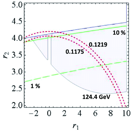
Figure 3: The Higgs boson mass, the degree of tuning a $\mu$-term, $|\Delta_{\mu}|\times 100(\%)$, and the relic abundance of the gravitino $\Omega_{3/2}h^{2}$ on the $(r_{1},r_{2})$-plane. In the blue shaded regions, the Higgs boson mass resides in the allowed range, $124.4\leq m_{h}\leq 126.8\,{\rm GeV}$ [1]. The green dashed and solid lines show the 1% and 10% tuning, respectively. The red dashed curves show the relic abundance of the gravitino within ranges $0.1179\leq\Omega_{3/2}h^{2}\leq 0.1215$, reported by the Planck Collaboration [22].

The ratios of gaugino masses at the GUT scale, $r_{1}$ and $r_{2}$, are severely constrained by the relic abundance of the gravitino as can be seen in Fig. 2. In this section, we show that the mass of the Higgs boson further constrains the ratios of gaugino masses, $r_{1}$ and $r_{2}$. The lightest CP-even Higgs boson corresponds to the SM-like Higgs in the framework of MSSM. Without the loop corrections, the Higgs boson mass is much lower than the observed mass of the Higgs reported by the LHC experiment [48]. Although, the high-scale SUSY-breaking scenario is a simple solution as one of the possibilities to raise the Higgs mass, it requires the tuning to obtain the EW vacuum. Therefore, we consider the maximal mixing of left- and right-handed top squarks to raise the Higgs boson mass without a severe fine-tuning.

With an approximation that the mass eigenstates of top squarks are nearly degenerate, the mass of the lightest CP-even Higgs boson cannot be realized. Thus, as pointed out in [2], we add the contribution from the mass differences between left- and right-handed top squarks in order to realize the observed Higgs boson mass and relax the degree of tuning at the same time. By employing the full one-loop RG equations of the MSSM from the GUT to the EW scale, we numerically calculate the Higgs boson mass which resides in the range of $124.4\leq m_{h}\leq 126.8$ [1], which is represented as the blue colored region in Fig. 3 and the degree of tuning a $\mu$-term, $|\Delta_{\mu}|\times 100\%$, is also given by the green dashed (1%) and solid lines (10%), respectively. From Fig. 3, there are the parameter spaces which are consistent with the relic abundance of the gravitino and the Higgs boson mass reported by the current cosmological observations [22] as well as the collider experiments [1] without a severe fine-tuning.

In particular, at the reference point $(r_{1},r_{2})=(6,3.5)$, the sparticle spectra, the Higgs boson mass $m_{h}$, and the degree of tuning a $\mu$-term $|\Delta_{\mu}|\times 100(\%)$ are summarized in Tables 4, 5, and 6. It is then satisfied by all the experimental lower bounds from the LHC experiments for the masses of all sparticles in Refs. [13] and [49] . In general, the SUSY flavor violations are dangerous in the gravity mediated SUSY-breaking scenario due to the flavor dependent interactions. In our setup, there are vanishing A-terms and no flavor dependent soft SUSY-breaking terms at the GUT scale because the moduli do not have the F-terms. Even if the moduli have the F-terms at the vacuum, the SUSY flavor violations can be suppressed from the structure of the $U(1)_{I^{\prime}}$ charge assignments [50]. Thus, there are no serious SUSY flavor violations; especially, the decay rates such as $\mu\rightarrow e\gamma$ and $b\rightarrow s\gamma$ evade the present limits [51, 52].

Sparticles	Mass[GeV]	Sparticles	Mass[GeV]
$\tilde{u}_{1}$	2618	$\tilde{e}_{1}$	3241
$\tilde{u}_{2}$	2359	$\tilde{e}_{2}$	2525
$\tilde{c}_{1}$	2520	$\tilde{\mu}_{1}$	2421
$\tilde{c}_{2}$	2011	$\tilde{\mu}_{2}$	2331
$\tilde{t}_{1}$	1735	$\tilde{\tau}_{1}$	2133
$\tilde{t}_{2}$	974	$\tilde{\tau}_{2}$	1447
$\tilde{d}_{1}$	2625	$\tilde{\nu}_{e_{1}}$	3240
$\tilde{d}_{2}$	2620	$\tilde{\nu}_{e_{2}}$	415
$\tilde{s}_{1}$	2522	$\tilde{\nu}_{\mu_{1}}$	2330
$\tilde{s}_{2}$	2189	$\tilde{\nu}_{\mu_{2}}$	415
$\tilde{b}_{1}$	2117	$\tilde{\nu}_{\tau_{1}}$	2132
$\tilde{b}_{2}$	1724	$\tilde{\nu}_{\tau_{2}}$	415
$\tilde{\chi}_{1}^{0}$	1723	$\tilde{\chi}_{1}^{\pm}$	444
$\tilde{\chi}_{2}^{0}$	1135	$\tilde{\chi}_{2}^{\pm}$	1723
$\tilde{\chi}_{3}^{0}$	448
$\tilde{\chi}_{4}^{0}$	441

Table 5: A typical sparticle spectra at the EW scale for the reference point, $(r_{1},r_{2})=(6,3.5)$. The subscripts denote the mass eigenvalues for the following: up ($\tilde{u}$), charm ($\tilde{c}$), top ($\tilde{t}$), down ($\tilde{d}$), strange ($\tilde{s}$), bottom ($\tilde{b}$) squarks, the scalar electron ($\tilde{e}$), muon ($\tilde{\mu}$), tauon ($\tilde{\tau}$), neutrino ($\tilde{\nu}$), the neutralino ($\tilde{\chi}$), and the chargino ($\tilde{\chi}^{\pm}$).

$m_{h}$[GeV]	$m_{H}$[GeV]	$m_{A}$[GeV]	$m_{H\pm}$[GeV]
125.4	1423	1423	1425
$\Delta_{\mu}^{-1}\times 100(\%)$	$M_{1}(m_{Z})$[GeV]	$M_{2}(m_{Z})$[GeV]	$M_{3}(m_{Z})$[GeV]
2.1	1133	1719	1575

Table 6: The neutral and charged Higgs boson masses $m_{h}$, $m_{H}$, $m_{A}$, and $m_{H_{\pm}}$, the degree of tuning a $\mu$-term, $|\Delta_{\mu}|\times 100(\%)$, and the gaugino masses at the EW scale for the reference point $(r_{1},r_{2})=(6,3.5)$.

5 Conclusion

In this paper, we proposed the gravitino dark matter in the gravity mediated SUSY-breaking scenario based on the $4$D ${\cal N}=1$ SUGRA. The nontrivial Kähler metric of the SUSY-breaking field induces the mass hierarchies between the gravitino and the other sparticles for any value of the F-term of the SUSY-breaking field. Especially, the small Kähler metric of the SUSY-breaking field leads to the stable gravitino of mass ${\cal O}(100)\,{\rm GeV}$ with TeV scale gauginos and sparticles which would be the typical features in the natural MSSM with gravity mediation, if the gauge kinetic functions and the kinetic terms of the matter fields satisfy certain conditions. (See Ref. [21] for the case of CMSSM.) In the stable gravitino scenario, one can consider the low-scale SUSY without the cosmological gravitino problem, only if the NLSP decays do not spoil the success of BBN.

As a concrete model, we considered the $5$D SUGRA model on $S^{1}/Z_{2}$. Since the successful inflation mechanism as well as the moduli stabilization have been realized in $5$D SUGRA [19, 22], we have estimated the moduli and inflaton decays into the gravitino dark matter. Although the produced gravitinos via the moduli decays seem to be dangerous from the cosmological point of view, their decays can be suppressed only if the moduli do not have the F-terms. Such a situation can be applied in our model, because the moduli, inflaton, and stabilizer fields have supersymmetric masses at the vacuum. Even if the supersymmetry is broken in the SUSY-breaking sector, their F-terms are suppressed by the gravitino mass at the SUSY-breaking minimum. When the NLSP and NNLSP are taken as the sneutrino and Higgsino-like neutralino, the nonthermal productions of the gravitino are negligible due to the small thermal abundance of the Higgsino-like neutralino. The smallness of the thermal abundance of NNLSP also relaxes the constraints from the BBN [10, 17, 47], and at the same time, the amount of neutrinos via the sneutrino decay can be suppressed. Thus, the total relic abundance of the gravitino is approximated by the thermal abundance of it which depends on the gaugino masses. As pointed out in [2], the certain ratios of gaugino masses are also important to raise the Higgs boson mass in the MSSM without a severe fine-tuning. From Fig. 3, it is found that certain ratios of gaugino masses are consistent with the relic abundance of the gravitino as well as the Higgs boson mass reported by the recent Planck and LHC data [1, 22].

In this paper, we focus on the $5$D SUGRA in order to show the realistic gravitino dark matter in the gravity mediation, and then the suppressed Kähler metric of the SUSY-breaking field is important to generate the mass hierarchies between the gravitino and other sparticles. When the $5$D SUGRA is derived as the effective theory of superstring theories on a warped throat and/or M-theory on the Calabi-Yau manifold [53], the SUSY-breaking sector would be constructed from the gauge theory living on Dp-branes and/or NS5-branes. Especially, in the type II string, the visible and hidden sectors can be realized on the different D-branes which wrap the certain cycles in the internal manifold. In such cases, the different volumes of the internal cycles lead to the hierarchical Kähler metric between the SUSY-breaking field and matter fields in the visible sector.

Acknowledgement

The author would like to thank H. Abe, T. Higaki, J. Kawamura, T. Kobayashi, and Y. Yamada for useful discussions and comments. H. O. was supported in part by a Grant-in-Aid for JSPS Fellows No. 26-7296.

Appendix A The F-terms of fields at the vacuum

In this appendix, we derive the F-terms of the moduli, stabilizer, and SUSY-breaking fields at the vacuum by employing the reference point method. As discussed in Sec. 3.3, when we expand the fields around the reference points given by Eqs. (16) and (21), $\phi\rightarrow\phi|_{\rm ref}+\delta\phi$, $\phi=T^{I^{\prime}},H_{i},X$ with $I^{\prime},i=1,2,3$, the Kähler metric with Kähler potentials (14) and (18) are expanded by

$$K_{I\bar{J}}=K_{I\bar{J}}^{(0)}+K_{I\bar{J}}^{(1)},$$ (99)

where

$$K_{I\bar{J}}^{(0)} =\begin{pmatrix}1/(2{\rm Re}T^{1})^{2}&0&0&0&0&0&0\\ 0&1/(2{\rm Re}T^{2})^{2}&0&0&0&0&0\\ 0&0&1/(2{\rm Re}T^{3})^{2}&0&0&0&0\\ 0&0&0&Z_{H_{1}}&0&0&0\\ 0&0&0&0&Z_{H_{2}}&0&0\\ 0&0&0&0&0&Z_{H_{3}}&0\\ 0&0&0&0&0&0&Z_{X}-4|X|^{2}/\Lambda^{2}\\ \end{pmatrix},$$ (100)

and

$$K_{I\bar{J}}^{(1)} =\begin{pmatrix}0&0&0&a_{H_{1}}H_{1}&0&0&a_{X}^{1}X\\ 0&0&0&0&a_{H_{2}}H_{2}&0&a_{X}^{2}X\\ 0&0&0&0&0&a_{H_{3}}H_{3}&a_{X}^{3}X\\ a_{H_{1}}\bar{H}_{1}&0&0&0&0&0&0\\ 0&a_{H_{2}}\bar{H}_{2}&0&0&0&0&0\\ 0&0&a_{H_{3}}\bar{H}_{3}&0&0&0&0\\ a_{X}^{1}\bar{X}&a_{X}^{2}\bar{X}&a_{X}^{3}X&0&0&0&0\\ \end{pmatrix},$$ (101)

in the field basis ($T^{1},T^{2},T^{3},H_{1},H_{2},H_{3},X$), with

$$a_{H_{i}}\equiv\cfrac{\partial Z_{H_{i}}}{\partial T^{I^{\prime}}}=\cfrac{1}{{\rm Re}T^{I^{\prime}}}\left(e^{-2c_{H_{i}}{\rm Re}T^{I^{\prime}}}-\cfrac{Z_{H_{i}}}{2}\right),\,\,\,(I^{\prime}=i),$$

$$a_{X}^{i}\equiv\cfrac{\partial Z_{X}}{\partial T^{I^{\prime}}}=\cfrac{c_{X}^{i}}{c_{X}\cdot{\rm Re}T}\left(e^{-2c_{X}\cdot ReT}-\cfrac{Z_{X}}{2}\right),$$

and the inverse of the Kähler metric is given by

$$K^{T^{I^{\prime}}\bar{T}^{I^{\prime}}}\simeq(2{\rm Re}T^{I^{\prime}})^{2}+8{\rm Re}T^{I^{\prime}}{\rm Re}\,\delta T^{I^{\prime}},\,\,\,K^{T^{I^{\prime}}\bar{H}_{i}}\simeq-A_{H_{i}}\delta H_{i},$$

$$K^{T^{I^{\prime}}\bar{X}}\simeq-A_{X}^{i}X-A_{X}^{i}\delta X,\,\,\,\,K^{H_{i}\bar{H}_{i}}\simeq\cfrac{1}{Z_{H_{i}}}-\cfrac{2a_{H_{i}}}{(Z_{H_{i}})^{2}}{\rm Re}\,\delta T^{I^{\prime}},$$

$$K^{X\bar{X}}\simeq\cfrac{1}{Z_{X}}-\cfrac{2a_{X}^{i}}{(Z_{X})^{2}}{\rm Re}\,\delta T^{I^{\prime}}+\cfrac{4}{\Lambda^{2}(Z_{X})^{2}}|\delta X|^{2},$$ (103)

where

$$A_{H_{i}}\equiv(2{\rm Re}T^{I^{\prime}})^{2}\cfrac{a_{H_{i}}}{Z_{H_{i}}},\,\,\,A_{X}^{i}\equiv(2{\rm Re}T^{I^{\prime}})^{2}\cfrac{a_{X}^{i}}{Z_{X}}.$$ (104)

Here and hereafter, we omit the subscript of $\phi$ at the reference point, that is, $\phi=\phi|_{\rm ref}$. From the relevant expansions in the scalar potential (1) with the Kähler and superpotential (14), (15), and (18),

$$D_{T^{I^{\prime}}}W \simeq K_{T^{I^{\prime}}}w,$$

$$+W_{T^{I^{\prime}}H_{i}}\delta H^{i}+K_{T^{I^{\prime}}{\bar{T}}^{I^{\prime}}}w(\delta T^{I^{\prime}}+\delta{\bar{T}}^{I^{\prime}})+K_{T^{I^{\prime}}}W_{X}\delta X$$

$$+W_{T^{I^{\prime}}T^{I^{\prime}}H_{i}}\delta T^{I^{\prime}}\delta H_{i}+\sum_{J^{\prime}=k}K_{T^{I^{\prime}}}W_{T^{J^{\prime}}H_{k}}\delta T^{k}\delta H^{k},$$

$$D_{H_{i}}W \simeq W_{T^{I^{\prime}}H_{i}}\delta T^{I^{\prime}}+K_{H_{i}{\bar{H}}_{i}}w\delta{\bar{H}}_{i}+\cfrac{W_{T^{I^{\prime}}T^{I^{\prime}}H_{i}}}{2}(\delta T^{I^{\prime}})^{2},$$

$$D_{X}W \simeq W_{X}+K_{X{\bar{X}}}w\delta{\bar{X}}+\frac{1}{2}\partial_{X}(K_{X\bar{X}})w(2|\delta X|^{2}+(\delta X)^{2}+(\delta\bar{X})^{2}),$$

$$W \simeq w+W_{X}\delta X+\sum_{I^{\prime}=i}^{3}W_{T^{I^{\prime}}H_{i}}\delta T^{I^{\prime}}\delta H_{i},$$

$$K \simeq\sum_{I^{\prime}=1}^{3}\left(-{\rm ln}({\rm Re}\,T^{I^{\prime}})-\cfrac{{\rm Re}\,\delta T^{I^{\prime}}}{{\rm Re}\,T^{I^{\prime}}}+\cfrac{1}{2}\left(\cfrac{{\rm Re}\,\delta T^{k}}{{\rm Re}\,T^{I^{\prime}}}\right)^{2}\right),$$ (105)

we obtain the scalar potential at the second order $\delta\phi$,

$$V \simeq\frac{W_{X}^{2}}{Z_{X}}-2wW_{X}(\delta X+\delta\bar{X})-\sum_{I^{\prime}=i}(2\text{Re}T^{I^{\prime}})wW_{T^{I^{\prime}}H_{i}}(\delta H_{i}+\delta\bar{H}_{i})$$

$$\hskip 13.0pt+\frac{4w^{2}}{\Lambda^{2}Z_{X}^{2}}|\delta X|^{2}+\sum_{I^{\prime}=i}\frac{W_{T^{I^{\prime}}H_{i}}^{2}}{Z_{H_{i}}}|\delta T^{I^{\prime}}|^{2}+\sum_{I^{\prime}=i}^{3}(2\text{Re}\,T^{I^{\prime}})^{2}W_{T^{I^{\prime}}H_{i}}^{2}|\delta H_{i}|^{2}$$

$$\hskip 13.0pt+\sum_{I^{\prime}=i}^{3}(-2\text{Re}\,T^{I^{\prime}}wW_{T^{I^{\prime}}T^{I^{\prime}}H_{i}}+wW_{T^{I^{\prime}}H_{i}})(\delta T^{I^{\prime}}\delta H_{i}+\delta\bar{T}^{I^{\prime}}\delta\bar{H}_{i})$$

$$\hskip 13.0pt+\sum_{I^{\prime}=i}\frac{A_{H_{i}}}{2\text{Re}T^{I^{\prime}}}wW_{T^{I^{\prime}}H_{i}}(\delta T^{I^{\prime}}\delta\bar{H}_{i}+\delta\bar{T}^{I^{\prime}}\delta H_{i})-\sum_{i=1}^{3}wW_{T^{I^{\prime}}H_{i}}(\delta T^{I^{\prime}}+\delta\bar{T}^{I^{\prime}})(\delta H_{i}+\delta\bar{H}_{i})$$

$$\hskip 13.0pt+\sum_{I^{\prime}=i}^{3}2\text{Re}\,T^{I^{\prime}}W_{X}W_{T^{I^{\prime}}H_{i}}(\delta H_{i}\delta\bar{X}+\delta\bar{H}_{i}\delta X)$$

$$\hskip 13.0pt+\sum_{I^{\prime}=i}^{3}\sum_{J^{\prime}=1}^{3}\frac{T^{I^{\prime}}+\bar{T}^{I^{\prime}}}{T^{J^{\prime}}+\bar{T}^{J^{\prime}}}wW_{T^{I^{\prime}}H_{i}}(\delta T^{J^{\prime}}+\delta\bar{T}^{J^{\prime}})(\delta H_{i}+\delta\bar{H}_{i}).$$ (106)

Finally, the extremal conditions for the relevant fields lead to the following variations of them:

$$\delta H_{i}\simeq\frac{w}{2\text{Re}T^{I^{\prime}}W_{T^{I^{\prime}}H_{i}}}\sim{\cal O}\left(\frac{m_{3/2}}{m_{H_{i}}}\right),\,\,\,\delta X\simeq\left(\frac{\Lambda^{2}Z_{X}^{2}}{4w^{2}}\right)5wW_{X},$$

$$\delta T^{I^{\prime}}\simeq\left(\frac{w}{W_{T^{I^{\prime}}H_{i}}}\right)^{2}Z_{H_{i}}\left(\frac{1+A_{H_{i}}K_{T^{I^{\prime}}}}{2\text{Re}T^{I^{\prime}}}+\frac{W_{T^{I^{\prime}}T^{I^{\prime}}H_{i}}}{W_{T^{I^{\prime}}H_{i}}}-\frac{3}{\text{Re}T^{I^{\prime}}}\right)\sim{\cal O}\left(\frac{m_{3/2}}{m_{T^{I^{\prime}}}}\right),$$ (107)

and their F-terms become

$$\sqrt{K_{T^{I^{\prime}}\bar{T}^{I^{\prime}}}}F^{T^{I^{\prime}}}=-e^{K/2}\sqrt{K_{T^{I^{\prime}}\bar{T}^{I^{\prime}}}}K^{T^{I^{\prime}}\bar{J}}\overline{D_{J}W}\sim O\left(\frac{m_{3/2}^{3}}{m_{T^{I^{\prime}}}^{2}}\right),$$

$$\sqrt{K_{H_{i}\bar{H}_{i}}}F^{H_{i}}=-e^{K/2}\sqrt{K_{H_{i}\bar{H}_{i}}}K^{H_{i}\bar{J}}\overline{D_{J}W}\sim O\left(\frac{m_{3/2}^{3}}{m_{H_{i}}^{2}}\right),$$

$$\sqrt{K_{X\bar{X}}}F^{X}\simeq-e^{K/2}\sqrt{K_{X\bar{X}}}K^{X\bar{X}}D_{X}W\simeq\frac{-W_{X}}{(\text{Re}T^{1}\text{Re}T^{2}\text{Re}T^{3})^{1/2}Z_{X}^{1/2}},$$ (108)

where

$$D_{T^{I^{\prime}}}W=\text{min}\left(O\left(\frac{m_{3/2}^{3}}{m_{T^{I^{\prime}}}^{2}}\right),O\left(\frac{m_{3/2}^{3}}{m_{X}^{2}}\right)\right),\,\,\,(I^{\prime}=1,2),$$

$$D_{T^{3}}W=O\left(\frac{m_{3/2}^{3}}{m_{T^{3}}^{2}}\right),\;\;D_{H_{i}}W=O\left(\frac{m_{3/2}^{2}}{m_{H_{i}}}\right),(i=1,2,3),\,\,\,D_{X}W\simeq\nu.$$ (109)

We also numerically checked these results, and then their F-terms can be suppressed by the tiny mass of the gravitino.

Appendix B The minima of fields during the inflation

By contrast, the minima of fields during the inflation are different from those at the true vacuum. In this section, we derive the minima of fields by employing the reference point method. The reference points of fields during the inflation are chosen in the same way as those at the vacuum. Similarly, we expand the fields except for the inflaton Re $T^{3}$ around the reference points given by Eqs. (16) and (21), $\phi\rightarrow\phi|_{\rm ref}+\delta\phi$, $\phi=T^{I^{\prime}},{\rm Im}\,T^{3},H_{i},X$ with $I^{\prime}=1,2$, $i=1,2,3$. It is then supposed that $H_{3}$ is fixed at the origin due to the Hubble-induced mass. From the scalar potential (1) with the Kähler and superpotentials (14), (15), and (18) given by the following expansions:

$$D_{T^{I^{\prime}}}W \simeq K_{T^{I^{\prime}}}w+W_{T^{I^{\prime}}H_{i}}\delta H_{i}+K_{T^{I^{\prime}}{\bar{T}}^{I^{\prime}}}w(\delta T^{I^{\prime}}+\delta{\bar{T}}^{I^{\prime}})+K_{T^{I^{\prime}}}(W_{H_{3}}\delta H_{3}+W_{X}\delta X)$$

$$+K_{T^{I^{\prime}}{\bar{T}}^{I^{\prime}}}W_{H_{3}}(\delta T^{I^{\prime}}+\delta{\bar{T}}^{I^{\prime}})\delta H^{3}+W_{T^{I^{\prime}}T^{I^{\prime}}H_{i}}\delta T^{I^{\prime}}\delta H_{i}+K_{T^{I^{\prime}}}\sum_{J^{\prime}=j}^{3}W_{T^{J^{\prime}}H^{j}}\delta T^{J^{\prime}}\delta H^{j},$$

$$D_{H_{1}}W \simeq W_{T^{1}H_{1}}\delta T^{1}+K_{H_{1}{\bar{H}}_{1}}w\delta{\bar{H}}_{1}+K_{H_{1}{\bar{H}}_{1}}W_{H_{3}}\delta{\bar{H}}_{1}\delta H_{3},$$

$$D_{H_{2}}W \simeq W_{T^{2}H_{2}}\delta T^{2}+K_{H_{2}{\bar{H}}_{2}}w\delta{\bar{H}}_{2}+K_{H_{2}{\bar{H}}_{2}}W_{H_{3}}\delta{\bar{H}}_{2}\delta H_{3},$$

$$D_{H_{3}}W \simeq W_{H_{3}}+W_{T^{3}H_{3}}\delta T^{3}+K_{H_{3}{\bar{H}}_{3}}W\delta{\bar{H}}_{3}+\partial_{T^{3}}(K_{H_{3}{\bar{H}}_{3}})w(\delta T^{3}+\delta{\bar{T}}^{3})\delta{\bar{H}}_{3},$$

$$+K_{H_{3}{\bar{H}}_{3}}(W_{H_{3}}|\delta H_{3}|^{2}+W_{X}\delta{\bar{H}}_{3}\delta X)+\cfrac{W_{T^{3}T^{3}H_{3}}}{2}(\delta T^{3})^{2},$$

$$D_{X}W \simeq W_{X}+K_{X{\bar{X}}}w\delta{\bar{X}}+\frac{1}{2}\partial_{X}(K_{X\bar{X}})w(2|\delta X|^{2}+(\delta X)^{2}+(\delta\bar{X})^{2})+K_{X{\bar{X}}}W_{H_{3}}\delta H_{3}\delta{\bar{X}},$$

$$W \simeq w+W_{X}\delta X+W_{H_{3}}\delta H_{3}+\sum_{I^{\prime}=i}^{3}W_{T^{I^{\prime}}H_{i}}\delta T^{I^{\prime}}\delta H_{i},$$

$$K \simeq\sum_{I^{\prime}=i}^{3}\left(-{\rm ln}{\rm Re}\,T^{I^{\prime}}-\cfrac{{\rm Re}\,\delta T^{I^{\prime}}}{{\rm Re}\,T^{I^{\prime}}}+\cfrac{1}{2}\left(\cfrac{{\rm Re}\,\delta T^{I^{\prime}}}{{\rm Re}\,T^{I^{\prime}}}\right)^{2}\right)+\sum_{i}Z_{H_{i}}|\delta H_{i}|^{2}+Z_{X}|\delta X|^{2},$$ (110)

we obtain the extremal conditions for the relevant fields, and then their variations become

$$\delta\tau^{1}=\delta\tau^{2}=\delta\tau^{3}=\delta k_{1}=\delta k_{2}=\delta k_{3}=\delta y=0,$$

$$\delta\sigma^{I^{\prime}}\sim O\left(\frac{Z_{H_{i}}}{W_{T^{I^{\prime}}H_{i}}^{2}\text{Re}\,T^{I^{\prime}}}\frac{|W_{H_{3}}|^{2}}{Z_{H_{3}}}\right)\simeq O\left(\left(\frac{H_{\rm inf}}{m_{T^{I^{\prime}}}}\right)^{2}\right),\,\,\,(I^{\prime}=1,2),$$

$$\delta h_{i}\sim O\left(\frac{K_{T^{I^{\prime}}}w}{W_{T^{I^{\prime}}H_{i}}(2\text{Re}T^{I^{\prime}})^{2}}\right)\simeq O\left(\frac{m_{3/2}}{m_{H_{i}}}\right),\,\,\,(i=1,2),$$

$$\delta h_{3}\sim O\left(\frac{w}{W_{H_{3}}}\right)\simeq O\left(\frac{m_{3/2}}{m_{H_{3}}}\right),$$

$$\delta x\sim O\left(\frac{\Lambda^{2}Z_{X}^{2}}{4W_{X}^{2}}W_{X}w\right)\simeq O\left(\left(\frac{m_{3/2}}{m_{X}}\right)^{2}\right),$$ (111)

where

$$\delta T^{I^{\prime}}\equiv\delta\sigma^{I^{\prime}}+i\delta\tau^{I^{\prime}},\;\;\delta H_{i}\equiv\delta h_{i}+i\delta k_{i},\;\;\delta X\equiv\delta x+i\delta y,$$ (112)

with $I^{\prime},i=1,2,3$.

References

- [1] G. Aad et al. [ATLAS Collaboration], Phys. Lett. B 716 (2012) 1 [arXiv:1207.7214 [hep-ex]], S. Chatrchyan et al. [CMS Collaboration], Phys. Lett. B 716 (2012) 30 [arXiv:1207.7235 [hep-ex]].
- [2] H. Abe, T. Kobayashi and Y. Omura, Phys. Rev. D 76 (2007) 015002 [hep-ph/0703044 [HEP-PH]], H. Abe, J. Kawamura and H. Otsuka, PTEP 2013 (2013) 013B02 [arXiv:1208.5328 [hep-ph]].
- [3] L. J. Hall, J. D. Lykken and S. Weinberg, Phys. Rev. D 27 (1983) 2359, S. K. Soni and H. A. Weldon, Phys. Lett. B 126 (1983) 215.
- [4] G. F. Giudice and R. Rattazzi, Phys. Rept. 322 (1999) 419 [hep-ph/9801271].
- [5] L. Randall and R. Sundrum, Nucl. Phys. B 557 (1999) 79 [hep-th/9810155], G. F. Giudice, M. A. Luty, H. Murayama and R. Rattazzi, JHEP 9812 (1998) 027 [hep-ph/9810442].
- [6] H. Pagels and J. R. Primack, Phys. Rev. Lett. 48 (1982) 223, S. Weinberg, Phys. Rev. Lett. 48 (1982) 1303.
- [7] M. Y. Khlopov and A. D. Linde, Phys. Lett. B 138 (1984) 265.
- [8] T. Moroi, H. Murayama and M. Yamaguchi, Phys. Lett. B 303 (1993) 289.
- [9] M. Kawasaki, K. Kohri and T. Moroi, Phys. Rev. D 71 (2005) 083502 [astro-ph/0408426]; K. Kohri, T. Moroi and A. Yotsuyanagi, Phys. Rev. D 73 (2006) 123511 [hep-ph/0507245].
- [10] T. Kanzaki, M. Kawasaki, K. Kohri and T. Moroi, Phys. Rev. D 75 (2007) 025011 [hep-ph/0609246], M. Kawasaki, K. Kohri, T. Moroi and A. Yotsuyanagi, Phys. Rev. D 78 (2008) 065011 [arXiv:0804.3745 [hep-ph]].
- [11] C. Kelso, S. Profumo and F. S. Queiroz, Phys. Rev. D 88 (2013) 2, 023511 [arXiv:1304.5243 [hep-ph]]; R. Allahverdi, B. Dutta, F. S. Queiroz, L. E. Strigari and M. Y. Wang, Phys. Rev. D 91 (2015) 5, 055033 [arXiv:1412.4391 [hep-ph]].
- [12] T. Moroi and L. Randall, Nucl. Phys. B 570 (2000) 455 [hep-ph/9906527].
- [13] G. Aad et al. [ATLAS Collaboration], JHEP 1410 (2014) 24 [arXiv:1407.0600 [hep-ex]].
- [14] K. Choi, K. S. Jeong and K. i. Okumura, JHEP 0509 (2005) 039 [hep-ph/0504037], M. Endo, M. Yamaguchi and K. Yoshioka, Phys. Rev. D 72 (2005) 015004 [hep-ph/0504036].
- [15] J. L. Feng, A. Rajaraman and F. Takayama, Phys. Rev. Lett. 91 (2003) 011302 [hep-ph/0302215], J. L. Feng, A. Rajaraman and F. Takayama, Phys. Rev. D 68 (2003) 063504 [hep-ph/0306024].
- [16] J. R. Ellis, K. A. Olive, Y. Santoso and V. C. Spanos, Phys. Lett. B 588 (2004) 7 [hep-ph/0312262].
- [17] J. L. Feng, S. f. Su and F. Takayama, Phys. Rev. D 70 (2004) 063514 [hep-ph/0404198].
- [18] H. Abe and H. Otsuka, JCAP 1411 (2014) 11, 027 [arXiv:1405.6520 [hep-th]].
- [19] N. Maru and N. Okada, Phys. Rev. D 70 (2004) 025002 [hep-th/0312148].
- [20] N. Arkani-Hamed and M. Schmaltz, Phys. Rev. D 61 (2000) 033005 [hep-ph/9903417], D. E. Kaplan and T. M. P. Tait, JHEP 0006 (2000) 020 [hep-ph/0004200].
- [21] J. Kersten and O. Lebedev, Phys. Lett. B 678 (2009) 481 [arXiv:0905.3711 [hep-ph]].
- [22] P. A. R. Ade et al. [Planck Collaboration], arXiv:1502.02114 [astro-ph.CO].
- [23] M. Zucker, Nucl. Phys. B 570 (2000) 267 [hep-th/9907082]; M. Zucker, JHEP 0008 (2000) 016 [hep-th/9909144]; M. Zucker, Phys. Rev. D 64 (2001) 024024 [hep-th/0009083]; M. Zucker, Fortsch. Phys. 51 (2003) 899.
- [24] T. Kugo and K. Ohashi, Prog. Theor. Phys. 105 (2001) 323 [hep-ph/0010288]; T. Fujita and K. Ohashi, Prog. Theor. Phys. 106 (2001) 221 [hep-th/0104130]; T. Fujita, T. Kugo and K. Ohashi, Prog. Theor. Phys. 106 (2001) 671 [hep-th/0106051]; T. Kugo and K. Ohashi, Prog. Theor. Phys. 108 (2002) 203 [hep-th/0203276].
- [25] H. Abe and Y. Sakamura, Phys. Rev. D 71 (2005) 105010 [hep-th/0501183], H. Abe and Y. Sakamura, Phys. Rev. D 73 (2006) 125013 [hep-th/0511208].
- [26] F. Paccetti Correia, M. G. Schmidt, Z. Tavartkiladze and , Nucl. Phys. B 751 (2006) 222 [hep-th/0602173].
- [27] H. Abe and Y. Sakamura, Phys. Rev. D 75 (2007) 025018 [hep-th/0610234].
- [28] H. Abe and Y. Sakamura, JHEP 0410 (2004) 013 [hep-th/0408224].
- [29] F. Paccetti Correia, M. G. Schmidt, Z. Tavartkiladze and , Nucl. Phys. B 709 (2005) 141 [hep-th/0408138],
- [30] Y. Sakamura, JHEP 1112 (2011) 008 [arXiv:1107.4247 [hep-th]].
- [31] Y. Sakamura, JHEP 1207 (2012) 183 [arXiv:1204.6603 [hep-th]].
- [32] Y. Sakamura, Nucl. Phys. B 873 (2013) 165 [Erratum-ibid. B 873 (2013) 728] [arXiv:1302.7244 [hep-th]], Y. Sakamura and Y. Yamada, JHEP 1311 (2013) 090 [Erratum-ibid. 1401 (2014) 181] [arXiv:1307.5585 [hep-th]].
- [33] H. Abe and Y. Sakamura, Nucl. Phys. B 796 (2008) 224 [arXiv:0709.3791 [hep-th]].
- [34] L. O’Raifeartaigh, Nucl. Phys. B 96 (1975) 331.
- [35] R. Kallosh and A. D. Linde, JHEP 0702 (2007) 002 [hep-th/0611183], R. Kitano, Phys. Lett. B 641 (2006) 203 [hep-ph/0607090].
- [36] H. Abe, T. Higaki, T. Kobayashi and Y. Omura, Phys. Rev. D 75 (2007) 025019 [hep-th/0611024].
- [37] A. A. Starobinsky, Phys. Lett. B 91 (1980) 99.
- [38] M. Endo, K. Hamaguchi and F. Takahashi, Phys. Rev. Lett. 96 (2006) 211301 [hep-ph/0602061].
- [39] S. Nakamura and M. Yamaguchi, Phys. Lett. B 638 (2006) 389 [hep-ph/0602081].
- [40] K. Nakayama, F. Takahashi and T. T. Yanagida, Phys. Lett. B 718 (2012) 526 [arXiv:1209.2583 [hep-ph]].
- [41] K. Choi, A. Falkowski, H. P. Nilles and M. Olechowski, Nucl. Phys. B 718 (2005) 113 [hep-th/0503216].
- [42] V. S. Kaplunovsky and J. Louis, Phys. Lett. B 306 (1993) 269 [hep-th/9303040].
- [43] R. Barbieri and G. F. Giudice, Nucl. Phys. B 306 (1988) 63.
- [44] M. Bolz, A. Brandenburg and W. Buchmuller, Nucl. Phys. B 606 (2001) 518 [Erratum-ibid. B 790 (2008) 336] [hep-ph/0012052].
- [45] J. Pradler and F. D. Steffen, Phys. Rev. D 75 (2007) 023509 [hep-ph/0608344].
- [46] M. Y. Khlopov, A. Barrau and J. Grain, Class. Quant. Grav. 23 (2006) 1875 [astro-ph/0406621].
- [47] K. Ishiwata, S. Matsumoto and T. Moroi, Phys. Rev. D 77 (2008) 035004 [arXiv:0710.2968 [hep-ph]].
- [48] Y. Okada, M. Yamaguchi and T. Yanagida, Prog. Theor. Phys. 85 (1991) 1.
- [49] J. Beringer et al. [Particle Data Group Collaboration], Phys. Rev. D 86 (2012) 010001.
- [50] H. Abe, H. Otsuka, Y. Sakamura and Y. Yamada, Eur. Phys. J. C 72 (2012) 2018 [arXiv:1111.3721 [hep-ph]].
- [51] J. Adam et al. [MEG Collaboration], Phys. Rev. Lett. 110 (2013) 201801 [arXiv:1303.0754 [hep-ex]].
- [52] Y. Amhis et al. [Heavy Flavor Averaging Group (HFAG) Collaboration], arXiv:1412.7515 [hep-ex].
- [53] A. Lukas, B. A. Ovrut, K. S. Stelle and D. Waldram, Phys. Rev. D 59 (1999) 086001 [hep-th/9803235], A. Lukas, B. A. Ovrut, K. S. Stelle and D. Waldram, Nucl. Phys. B 552 (1999) 246 [hep-th/9806051].