Quasiprobability distributions in open quantum systems: spin-qubit systems

Abstract

We study nonclassical features in a number of spin-qubit systems including single, two and three qubit states, as well as an $N$ qubit Dicke model and a spin-1 system, of importance in the fields of quantum optics and information. This is done by analyzing the behavior of the well known Wigner, $P$, and $Q$ quasiprobability distributions on them. We also discuss the not so well known $F$ function and specify its relation to the Wigner function. Here we provide a comprehensive analysis of quasiprobability distributions for spin-qubit systems under general open system effects, including both pure dephasing as well as dissipation. This makes it relevant from the perspective of experimental implementation.

PACS: 03.65.Yz,03.75.Be,42.50.-p

I Introduction

A very useful concept in the analysis of the dynamics of classical systems is the notion of phase space. A straightforward extension of this to the realm of quantum mechanics is however foiled due to the uncertainty principle. Despite this, it is possible to construct quasiprobability distributions (QDs) for quantum mechanical systems in analogy with their classical counterparts (KS, ; SZ, ; Sch, ; GSA, ; Puri, ; Klimnov, ). These QDs are very useful in that they provide a quantum classical correspondence and facilitate the calculation of quantum mechanical averages in close analogy to classical phase space averages. Nevertheless, the QDs are not probability distributions as they can take negative values as well, a feature that could be used for the identification of quantumness in a system.

The first such QD was developed by Wigner resulting in the epithet Wigner function ($W$) (wig, ; moyal, ; hillery, ; kimnoz, ; adam1, ; adam2, ). Another, very well known, QD is the $P$ function whose development was a precursor to the evolution of the field of quantum optics. This was originally developed from the possibility of expressing any state of the radiation field in terms of a diagonal sum over coherent states (glaub, ; sudar, ). The $P$ function can become singular for quantum states, a feature that promoted the development of other QDs such as the $Q$ function (mehta, ; kano, ; husimi, ) as well as further highlighted the use of the $W$ function which does not have this feature. These QDs are intimately related to the problem of operator orderings. Thus, the $P$ and $Q$ functions are related to the normal and antinormal orderings, respectively, while the $W$ function is associated with symmetric operator ordering. It is quite clear that there can be other QDs, apart from the above three, depending upon the operator ordering. However, among all the possible QDs the above three QDs are the most widely studied. There exist several reasons behind the intense interest in these QDs. They can be used to identify the nonclassical (quantum) nature of a state referee . Specifically, nonpositive values of $P$ function define a nonclassical state. Nonpositivity of $P$ is a necessary and sufficient criterion for nonclassicality, but other QDs provide only sufficient criteria.

A nonclassical state can be used to perform tasks that are classically impossible. This fact motivated many studies on nonclassical states, for example, studies on squeezed, antibunched and entangled states. The interest on nonclassical states has been considerably amplified in the recent past after the advent of quantum information where several applications of nonclassical states, in particular, of entangled states, have been reported (my book, ). Interestingly many of these applications have been designed using spin-qubit systems.

Quantum optics deals with atom-field interactions. The atoms, in their simplest forms, are modeled as qubits (two-level systems). These are also of immense practical importance as they can be the effective realizations of Rydberg atoms (sa, ; ga, ). Atomic systems are also studied in the context of the Dicke model (dicke, ; dowling, ), a collection of two-level atoms; in atomic traps (we, ), atomic interferometers (kita, ), polarization optics (kara, ), and have recently found applications in quantum computation ((Qu-comp1, ; Qu-comp2, ; Qu-comp3, ; Qu-comp4, ; Qu-comp5, ; Qu-comp6, ) and references therein) as well as in the generation of long-distance entanglement (Qu-comp7, ). All these would evoke the question whether one could have QDs for such atomic systems as well. Such questions, which are of relevance to the present work, would be closely tied to the problem of development of QDs for $SU(2)$, spin-like (spin-$j$), systems. Such a development was made in (strato, ), where a QD on the sphere, naturally related to the $SU(2)$ dynamical group (klim, ; chuma, ), was obtained. There are by now a number of constructions of spin QDs (wootters, ; vourdas, ; chatur, ; leon, ; paz, ), among others.

However, another approach, the one adapted here, is to make use of the connection of $SU(2)$ geometry to that of a sphere. The spherical harmonics provide a natural basis for functions on the sphere. This, along with the general theory of multipole operators (blum, ; zare, ), can be made use of to construct QDs of spin (qubit) systems as functions of polar and azimuthal angles (agarwal, ). Other constructions, in the literature, of $W$ functions for spin-$1/2$ systems can be found in (cohen, ; varilly, ), among others. A concept that played an important role in the above developments, was the atomic coherent state (arecchi, ), which lead to the definition of atomic $P$ function in close analogy to their radiation field counterparts. Another related development, following (mh, ) where joint probability distributions were obtained for spin-1 systems exposed to quadrupole fields, was a QD obtained from the Fourier inversion of the characteristic function of the corresponding probability mass function, using the Wigner-Weyl correspondence. This could be called the characteristic function or $F$-function approach (rama, ).

The fields of quantum optics and information have matured to the point where intense experimental investigations are being made. Both from the fundamental perspective as well as from the viewpoint of practical realizations, it is imperative to study the evolution of the system of interest taking into account the effect of its ambient environment. This is achieved systematically by using the formalism of Open Quantum Systems (louis, ; bp, ; pi, ; sbqbm, ).

In the present work, we investigate nonclassicality in a number of spin-qubit systems including single, two and three qubit states, as well as $N$ qubit Dicke states and a spin-1 system, of importance in the fields of quantum optics and information. This is done by analyzing the behavior of the well known $W$, $P$, $Q$ QDs on them. The significance of this is rooted to the phenomena of quantum state engineering, which involves the generation and manipulation of nonclassical states (adam-SE, ; SE-nature, ). In this context, it is imperative to have an understanding over quantum to classical transitions, under ambient conditions. Such an understanding is made possible by the present work, where investigations are done in the presence of open system effects, both purely dephasing (decoherence) (sbsrikgp, ; QND, ), also known as quantum non-demolition (QND), as well as dissipation (sbsrikgp, ; SGAD, ). These aspects of open system evolution have been realized in a series of beautiful experiments (haroche, ; turchette, ). We also discuss the not so well known $F$ function and specify its relation to the $W$ function. Further, we expect this work to have an impact on tomography related issues, as borne out in (agarwal98, ), where a method for quantum state reconstruction of a system of spins or qubits was proposed using the $Q$ function. Also, the $Q$ function, studied here, can be turned to address fundamental issues such as complementarity between number and phase distributions (shapiro, ; hall, ; agarwalphase, ), under the influence of QND as well as dissipative interactions with their environment, as well as for phase dispersion in atomic systems (sbphase, ; sbsrik, ). Here, to the best of our knowledge, we provide, for the first time, a comprehensive analysis of QDs for spin-qubit systems under general open system effects.

The plan of this paper is as follows. In the next section, we will briefly discuss the QDs that will be subsequently used in the rest of the work, i.e., the $W$, $P$, $Q$, and $F$ functions. This will be followed by a study of open system QDs for single qubit states. Next, we take up the case of some interesting two and three qubit states as well as the well known $N$ qubit Dicke model. We then discuss, briefly, QDs of a spin-1 system. These examples will provide an understanding of quantum to classical transitions as indicated by the various QDs, under general open system evolutions. Although QDs have been frequently used to identify the existence of nonclassical states (perina-book, ), they do not directly provide any quantitative measure of the amount of nonclassicality. Keeping these in mind, several measures of nonclassicality have been proposed, but all of them are seen to suffer from some limitations (with-adam-meas, ). A specific measure of nonclassicality is the nonclassical volume, which considers the doubled volume of the integrated negative part of the $W$ function as a measure of nonclassicality (zyco, ). In the penultimate section, we make a study of quantumness, in some of the systems considered in this work, by using nonclassical volume (zyco, ). We then make our conclusions.

II Distribution functions for spin (qubit) systems

Here, we briefly discuss the different QDs, i.e., the $W$, $P$, $Q$, and $F$ functions, subsequently used in the paper.

II.1 The Wigner function

Exploiting the connection between spin-like, $SU(2)$, systems and the sphere, a QD can be expressed as a function of the polar and azimuthal angles. This expanded over a complete basis set, a convenient one being the spherical harmonics, the $W$ function for a single spin-$j$ state can be expressed as (agarwal, )

$$\begin{array}[]{lcl}W\left(\theta,\phi\right)&=&\left(\frac{2j+1}{4\pi}\right)^{1/2}\underset{K,Q}{\sum}\rho_{KQ}Y_{KQ}\left(\theta,\phi\right),\end{array}$$ (1)

where $K=0,1,\ldots,2j$, and $Q=-K,-K+1,\ldots,0,\ldots,K-1,K$, and

$$\begin{array}[]{lcl}\rho_{KQ}&=&Tr\left\{T_{KQ}^{\dagger}\rho\right\}.\end{array}$$ (2)

Here, $Y_{KQ}$ are spherical harmonics and $T_{KQ}$ are multipole operators given by

$$\begin{array}[]{lcl}T_{KQ}&=&\underset{m,m^{\prime}}{\sum}\left(-1\right)^{j-m}\left(2K+1\right)^{1/2}\left(\begin{array}[]{ccc}j&K&j\\ -m&Q&m^{\prime}\end{array}\right)|j,m\rangle\langle j,m^{\prime}|,\end{array}$$ (3)

where $\left(\begin{array}[]{ccc}j_{1}&j_{2}&j\\ m_{1}&m_{2}&m\end{array}\right)=\frac{\left(-1\right)^{j_{1}-j_{2}-m}}{\sqrt{2j+1}}\langle j_{1}m_{1}j_{2}m_{2}|j-m\rangle$ is the Wigner $3j$ symbol (varshalo, ) and $\langle j_{1}m_{1}j_{2}m_{2}|j-m\rangle$ is the Clebsh-Gordon coefficient. The multipole operators $T_{KQ}$ are orthogonal to each other and they form a complete set with property $T_{KQ}^{\dagger}=\left(-1\right)^{Q}T_{K,-Q}$. The $W$ function is normalized as

$$\int W\left(\theta,\phi\right)\sin\theta d\theta d\phi=1,$$

and $W^{*}\left(\theta,\phi\right)=W\left(\theta,\phi\right)$. Similarly, the $W$ function of a two particle system, each with spin-$j$ is (agarwal, ; rama, )

$$\begin{array}[]{lcl}W\left(\theta_{1},\phi_{1},\theta_{2},\phi_{2}\right)&=&\left(\frac{2j+1}{4\pi}\right)\underset{K_{1},Q_{1}}{\sum}\underset{K_{2},Q_{2}}{\sum}\rho_{K_{1}Q_{1}K_{2}Q_{2}}Y_{K_{1}Q_{1}}\left(\theta_{1},\phi_{1}\right)Y_{K_{2}Q_{2}}\left(\theta_{2},\phi_{2}\right),\end{array}$$ (4)

where $\begin{array}[]{lcl}\rho_{K_{1}Q_{1}K_{2}Q_{2}}&=&Tr\left\{\rho T_{K_{1}Q_{1}}^{\dagger}T_{K_{2}Q_{2}}^{\dagger}\right\}.\end{array}$ Here, $W\left(\theta_{1},\phi_{1},\theta_{2},\phi_{2}\right)$ is also normalized as

$$\int W\left(\theta_{1},\phi_{1},\theta_{2},\phi_{2}\right)\sin\theta_{1}\sin\theta_{2}d\theta_{1}d\phi_{1}d\theta_{2}d\phi_{2}=1.$$

Further, it is known that any arbitrary operator can be mapped into the $W$ function or any other QD discussed here. In what follows, using the same notations we describe $P$, $Q$ and $F$ functions for single spin-$j$ state and for two spin-$j$ particles. It may be noted that all the analytic expressions for the QDs given below are normalized.

II.2 The $P$ function

In analogy with the $P$ function for continuous variable systems, the $P$ function for a single spin-$j$ state is defined as agarwal

$$\rho=\int d\theta d\phi P\left(\theta,\phi\right)|\theta,\phi\rangle\langle\theta,\phi|,$$ (5)

and can be shown to be

$$\begin{array}[]{lcl}P\left(\theta,\phi\right)&=&\underset{K,Q}{\sum}\rho_{KQ}Y_{KQ}\left(\theta,\phi\right)\left(\frac{1}{4\pi}\right)^{1/2}\left(-1\right)^{K-Q}\left(\frac{\left(2j-K\right)!\left(2j+K+1\right)!}{\left(2j\right)!\left(2j\right)!}\right)^{1/2}.\end{array}$$ (6)

The $P$ function for two spin-$j$ particles is (agarwal, ; rama, )

$$\begin{array}[]{lcl}P\left(\theta_{1},\phi_{1},\theta_{2},\phi_{2}\right)&=&\underset{K_{1},Q_{1}}{\sum}\underset{K_{2},Q_{2}}{\sum}\rho_{K_{1}Q_{1}K_{2}Q_{2}}Y_{K_{1}Q_{1}}\left(\theta_{1},\phi_{1}\right)Y_{K_{2}Q_{2}}\left(\theta_{2},\phi_{2}\right)\\ &\times&\left(-1\right)^{K_{1}-Q_{1}+K_{2}-Q_{2}}\left(\frac{1}{4\pi}\right)\left(\frac{\sqrt{\left(2j-K_{1}\right)!\left(2j-K_{2}\right)!\left(2j+K_{1}+1\right)!\left(2j+K_{2}+1\right)!}}{\left(2j\right)!\left(2j\right)!}\right).\end{array}$$ (7)

Here $|\theta,\phi\rangle$ is the atomic coherent state (arecchi, ) and can be expressed in terms of the Wigner-Dicke states $|j,m\rangle$ as

$$|\theta,\phi\rangle=\underset{m=-j}{\sum^{j}}\left(\begin{array}[]{c}2j\\ m+j\end{array}\right)^{1/2}\sin^{j+m}(\frac{\theta}{2})\cos^{j-m}(\frac{\theta}{2})e^{-i(j+m)\phi}|j,m\rangle.$$ (8)

II.3 The $Q$ function

Similarly, the $Q$ function for a single spin-$j$ state is

$$Q\left(\theta,\phi\right)=\frac{2j+1}{4\pi}\langle\theta,\phi|\rho|\theta,\phi\rangle,$$ (9)

and can be expressed as agarwal

$$\begin{array}[]{lcl}Q\left(\theta,\phi\right)&=&\underset{K,Q}{\sum}\rho_{KQ}Y_{KQ}\left(\theta,\phi\right)\left(\frac{1}{4\pi}\right)^{1/2}\left(-1\right)^{K-Q}\left(2j+1\right)\left(\frac{\left(2j\right)!\left(2j\right)!}{\left(2j-K\right)!\left(2j+K+1\right)!}\right)^{1/2}.\end{array}$$ (10)

Further, the normalized $Q$ function for two particle system of spin-$j$ (agarwal, ; rama, ) particles is

$$\begin{array}[]{lcl}Q\left(\theta_{1},\phi_{1},\theta_{2},\phi_{2}\right)&=&\underset{K_{1},Q_{1}}{\sum}\underset{K_{2},Q_{2}}{\sum}\rho_{K_{1}Q_{1}K_{2}Q_{2}}Y_{K_{1}Q_{1}}\left(\theta_{1},\phi_{1}\right)Y_{K_{2}Q_{2}}\left(\theta_{2},\phi_{2}\right)\left(\frac{\left(2j+1\right)^{2}}{4\pi}\right)\\ &\times&\left(-1\right)^{K_{1}-Q_{1}+K_{2}-Q_{2}}\left(\frac{\left(2j\right)!\left(2j\right)!}{\sqrt{\left(2j-K_{1}\right)!\left(2j-K_{2}\right)!\left(2j+K_{1}+1\right)!\left(2j+K_{2}+1\right)!}}\right).\end{array}$$ (11)

II.4 The $F$ function

The $F$ distribution function (rama, ) is defined using the relation between Fano statistical tensors and state multipole operators. Specifically, for a single spin-$j$ state, it is defined as (rama, )

$$\begin{array}[]{lcl}F\left(\theta,\phi\right)&=&\underset{K,Q}{\sum}\rho_{KQ}Y_{KQ}\left(\theta,\phi\right)\left(\frac{1}{4\pi}\right)^{1/2}\frac{1}{2^{K}}\left(\frac{\left(2j+K+1\right)!}{\left(2j-K\right)!\left\{j\left(j+1\right)\right\}^{K}}\right)^{1/2}.\end{array}$$ (12)

Similarly, the normalized $F$ function for a two particle, spin-$j$, (rama, ) system is

$$\begin{array}[]{lcl}F\left(\theta_{1},\phi_{1},\theta_{2},\phi_{2}\right)&=&\underset{K_{1},Q_{1}}{\sum}\underset{K_{2},Q_{2}}{\sum}\rho_{K_{1}Q_{1}K_{2}Q_{2}}Y_{K_{1}Q_{1}}\left(\theta_{1},\phi_{1}\right)Y_{K_{2}Q_{2}}\left(\theta_{2},\phi_{2}\right)\\ &\times&\left(\frac{1}{4\pi\left(2^{K_{1}+K_{2}}\right)}\right)\left(\frac{\left(2j+K_{1}+1\right)!\left(2j+K_{2}+1\right)!}{\left(2j-K_{1}\right)!\left(2j-K_{2}\right)!\left\{j\left(j+1\right)\right\}^{K_{1}+K_{2}}}\right)^{1/2}.\end{array}$$ (13)

To summarize, all the QDs discussed in this work are normalized to unity. They are also real functions as they correspond to probability density functions for classical states. The density matrix of a quantum state can be reconstructed from these QDs (Klimnov, ). One can also calculate the expectation value of an operator from them (agarwal, ).

It would be appropriate here to make a brief comparison of the QDs, discussed above, with their continuous variable counterparts. The coherent state and thereby the displacement operator $D$, which generate coherent states from vacuum and is usually expressed as $D(\phi)=e^{\phi\hat{a}^{\dagger}-\phi^{*}\hat{a}}$ with $\hat{a}$, $\hat{a}^{\dagger}$ being the annihilation and creation operators of the given Fock space, respectively, play a central role in these considerations. Thus, for example, the Wigner function, associated with a state $\rho$ is the symplectic Fourier transform of the mean value of $D$ in the state $\rho$, leading to the standard representation of the Wigner function as the Fourier transform of the skewed matrix representation of $\rho$,

$$W(\eta,\overline{\eta})=\frac{1}{2\pi}\int_{-\infty}^{\infty}d\xi\langle a-\frac{\xi}{2}|\rho|a+\frac{\xi}{2}\rangle e^{i\xi b},$$ (14)

with $a$ and $b$ being real and $\eta=\frac{1}{\sqrt{2}}(a+ib)$. Similarly, the $P$ function is associated with the diagonal representation of the state $\rho$ in terms of the coherent state, while the $Q$ function is related to the expectation value of $\rho$, with respect to coherent states.

The multipole operators $T_{KQ}$ (3) play a pivotal role in the construction of QDs of spin systems, discussed here. These operators are extensively used in the study of atomic and nuclear radiation and can be shown to have properties analogous to those of the coherent state dispalcement operator $D$ for usual continuous variable bosonic systems (agarwal, ). In this sense, the properties of spin QDs are analogous to those of their continuous variable counterparts, with the atomic coherent state playing the role of the usual coherent state. Thus, for example, even though, for the spin (qubit) systems, both $P$ and $W$ QDs are witnesses of quantum correlations, in the sense that their negative values indicate quantumnes in the system, it is possible for a scenario wherein the $P$ function is negative and $W$ is positive, but not viceversa. The $Q$ function is always positive, while the $F$ function is same as the $W$ function for spin-$\frac{1}{2}$ systems, as shown below.

Before proceeding further, it is worth noting here that for all the spin-$\frac{1}{2}$ states (qubits), single or multi-qubit, the $W$ and $F$ QDs are identical. Specifically, for the single qubit case, the $W$ function is

$$W_{\frac{1}{2}}\left(\theta,\phi\right)=\frac{1}{\sqrt{2\pi}}\underset{K,Q}{\sum}M_{K,Q}\left(\theta,\phi\right),$$

where $M_{K,Q}\left(\theta,\phi\right)=\rho_{KQ}Y_{KQ}\left(\theta,\phi\right)$, while, the $F$ function is

$$F_{\frac{1}{2}}\left(\theta,\phi\right)=\frac{1}{\sqrt{4\pi}}\underset{K,Q}{\sum}M_{K,Q}\left(\theta,\phi\right)\left(\frac{\left(2+K\right)!}{3^{K}\left(1-K\right)!}\right)^{1/2},$$

where the term inside the brackets with square root is $2$ for both the values of $K$ (i.e., $0$ or $1$). Similarly, for two spin-$\frac{1}{2}$ states, the $W$ and $F$ functions are

$$\begin{array}[]{lcl}F_{\frac{1}{2},\frac{1}{2}}\left(\theta_{1},\phi_{1},\theta_{2},\phi_{2}\right)&=&\frac{1}{4\pi}\underset{K_{1},Q_{1}}{\sum}\underset{K_{2},Q_{2}}{\sum}M_{K_{1}Q_{1}K_{2}Q_{2}}\left(\theta_{1},\phi_{1},\theta_{2},\phi_{2}\right)\left(\frac{\left(2+K_{1}\right)!\left(2+K_{2}\right)!}{3^{K_{1}+K_{2}}\left(1-K_{1}\right)!\left(1-K_{2}\right)!}\right)^{1/2}\\ &=&\frac{1}{2\pi}\underset{K_{1},Q_{1}}{\sum}\underset{K_{2},Q_{2}}{\sum}M_{K_{1}Q_{1}K_{2}Q_{2}}\left(\theta_{1},\phi_{1},\theta_{2},\phi_{2}\right)\\ &=&W_{\frac{1}{2},\frac{1}{2}}\left(\theta_{1},\phi_{1},\theta_{2},\phi_{2}\right),\end{array}$$

where $M_{K_{1}Q_{1}K_{2}Q_{2}}\left(\theta_{1},\phi_{1},\theta_{2},\phi_{2}\right)=\rho_{K_{1}Q_{1}K_{2}Q_{2}}Y_{K_{1}Q_{1}}\left(\theta_{1},\phi_{1}\right)Y_{K_{2}Q_{2}}\left(\theta_{2},\phi_{2}\right),$ and the term in the brackets is $4$ for all the possible values of $K_{1}$ and $K_{2}$. This can further be extended for higher number of spin-$\frac{1}{2}$ states.

Since the $W$ and $F$ functions are the same for spin-$\frac{1}{2}$ systems, we will not discuss the evolution of the $F$ function of these systems.

III Distribution functions for single spin-$\frac{1}{2}$ states

Here, we consider single spin-$\frac{1}{2}$ states, initially in an atomic coherent state, in the presence of two different noises, i.e., QND (sbsrikgp, ; QND, ), which are purely dephasing, and the dissipative SGAD (Squeezed Generalized Amplitude Damping) (sbsrikgp, ; SGAD, ) noises. For calculating the QDs, we will require multipole operators for $j=\frac{1}{2}$ and $m,\,m^{\prime}=\pm\frac{1}{2}$, giving $K=0$ and $1$. For $K=0$, $Q=0$, and for $K=1$, $Q=1,\,0,\,-1$. Using these, the multipole operators $T_{KQ}$ can be obtained as $\begin{array}[]{lcl}T_{00}&=&\frac{1}{\sqrt{2}}\left[\begin{array}[]{cc}1&0\\ 0&1\end{array}\right],\end{array}$ $\begin{array}[]{lcl}T_{11}&=&\left[\begin{array}[]{cc}0&0\\ -1&0\end{array}\right],\end{array}$ $\begin{array}[]{lcl}T_{10}&=&\frac{1}{\sqrt{2}}\left[\begin{array}[]{cc}1&0\\ 0&-1\end{array}\right],\end{array}$and $\begin{array}[]{lcl}T_{1-1}&=&\left[\begin{array}[]{cc}0&1\\ 0&0\end{array}\right].\end{array}$

III.1 Atomic coherent state in QND noise

The master equation of the system interacting with a squeezed thermal bath and undergoing a QND evolution (QND, ) is

$$\begin{array}[]{lcl}\dot{\rho}{}_{nm}\left(t\right)&=&\left[-\frac{i}{\hbar}\left(E_{n}-E_{m}\right)+i\dot{\eta}\left(t\right)\left(E_{n}^{2}-E_{m}^{2}\right)-\left(E_{n}-E_{m}\right)^{2}\dot{\gamma}\left(t\right)\right]\rho_{nm}\left(t\right),\end{array}$$ (15)

where $E_{n}$s are the eigenvalues of the system Hamiltonian in the system eigenbasis $|n\rangle$, which here would correspond to the Wigner-Dicke states (GSA, );

$$\eta\left(t\right)=-\underset{k}{\sum}\frac{g_{k}^{2}}{\hbar^{2}\omega_{k}^{2}}\sin\left(\omega_{k}t\right)$$

and

$$\begin{array}[]{lcl}\gamma\left(t\right)&=&\frac{1}{2}\underset{k}{\sum}\frac{g_{k}^{2}}{\hbar^{2}\omega_{k}^{2}}\coth\left(\frac{\beta\hbar\omega_{k}}{2}\right)\left|\left(e^{i\omega_{k}t}-1\right)\cosh\left(r_{k}\right)+\left(e^{-i\omega_{k}t}-1\right)\sinh\left(r_{k}\right)e^{2i\Phi_{k}}\right|^{2}.\end{array}$$

Here, $\beta=\frac{1}{k_{B}T}$, and $k_{B}$ is the Boltzmann constant, while $r_{k}$ and $\Phi_{k}$ are the squeezing parameters. The initial density matrix for the atomic coherent state is

$$\rho\left(0\right)=|\alpha,\beta\rangle\langle\alpha,\beta|,$$ (16)

where $|\alpha,\beta\rangle$ is given by Eq. (8). The density matrix (16) in the presence of QND noise at time $t$ becomes

$$\begin{array}[]{lcl}\rho_{jm,jn}\left(t\right)&=&e^{-i\omega\left(m-n\right)t}e^{i\left(\hbar\omega\right)^{2}\left(m^{2}-n^{2}\right)\eta\left(t\right)}e^{-\left(\hbar\omega\right)^{2}\left(m-n\right)^{2}\gamma\left(t\right)}\rho_{jm,jn}\left(0\right),\end{array}$$ (17)

where

$$\begin{array}[]{lcl}\rho_{jm,jn}\left(0\right)&=&\langle j,m|\rho\left(0\right)|j,n\rangle\\ &=&\langle j,m|\alpha,\beta\rangle\langle\alpha,\beta|j,n\rangle.\end{array}$$ (18)

For $j=\frac{1}{2}$, the initial density matrix is

$$\rho\left(0\right)=\left[\begin{array}[]{cc}\sin^{2}\left(\frac{\alpha}{2}\right)&\frac{1}{2}e^{-i\beta}\sin\alpha\\ \frac{1}{2}e^{i\beta}\sin\alpha&\cos^{2}\left(\frac{\alpha}{2}\right)\end{array}\right],$$ (19)

which in the presence of QND noise becomes

$$\rho\left(t\right)=\left[\begin{array}[]{cc}\sin^{2}\left(\frac{\alpha}{2}\right)&\frac{1}{2}e^{-i\omega t}e^{-\left(\hbar\omega\right)^{2}\gamma\left(t\right)}e^{-i\beta}\sin\alpha\\ \frac{1}{2}e^{i\omega t}e^{-\left(\hbar\omega\right)^{2}\gamma\left(t\right)}e^{i\beta}\sin\alpha&\cos^{2}\left(\frac{\alpha}{2}\right)\end{array}\right].$$ (20)

Here, we consider the case of an Ohmic bath for which analytic expressions for $\gamma\left(t\right)$, both for zero and high temperatures, can be obtained (QND, ). These are functions of the bath parameters $\gamma_{0}$ and $\omega_{c}$ as well as squeezing parameters $r$ and $\phi$, with $\phi=a\omega$ and $a$ is a constant dependent on the squeezed bath. Now, using multipole operators, mentioned above, analytic expressions of the different QDs can be obtained. For example, we have obtained the $W$ function for a qubit, starting from an atomic coherent state, in the presence of QND noise as

$$\begin{array}[]{lcl}W\left(\theta,\phi\right)&=&\frac{1}{4\pi}\left(1-\sqrt{3}\cos\alpha\cos\theta+\sqrt{3}e^{-\left(\hbar\omega\right)^{2}\gamma\left(t\right)}\cos\left(\beta+\omega t+\phi\right)\sin\alpha\sin\theta\right),\end{array}$$ (21)

while, the corresponding $P$ and $Q$ QDs are obtained as

$$\begin{array}[]{lcl}P\left(\theta,\phi\right)&=&\frac{1}{4\pi}\left(1+3\cos\alpha\cos\theta+3e^{-\left(\hbar\omega\right)^{2}\gamma\left(t\right)}\cos\left(\beta+\omega t+\phi\right)\sin\alpha\sin\theta\right),\end{array}$$ (22)

and

$$\begin{array}[]{lcl}Q\left(\theta,\phi\right)&=&\frac{1}{4\pi}\left(1+\cos\alpha\cos\theta+e^{-\left(\hbar\omega\right)^{2}\gamma\left(t\right)}\cos\left(\beta+\omega t+\phi\right)\sin\alpha\sin\theta\right),\end{array}$$ (23)

respectively. All the QDs calculated in Eqs. (21)-(23) can be used to get the corresponding noiseless QDs for the same system and this also serves as a nice consistency check of the calculations. The variation of the QDs, Eqs. (21)-(23), for some specific parameter values are shown in Fig. 1 a-c, where the effect of the presence of noise on the QDs can be easily observed. Both the $P$ and $W$ functions are found to exhibit negative values indicative of quantumness in the system. Also, in Fig. 1 b-c, we can see that with an increase in temperature $T$, the QDs tend to become less negative, which is an indicator of a move towards classicality, as expected. Interestingly, in Fig. 1 a, we do not observe any zero of the $Q$ function which implies that the $Q$ function does not show any signature of nonclassicality in this particular case. The oscillatory nature of the QDs for atomic coherent state when subjected to QND noise can be attributed to the purely dephasing effect of the QND interaction. That is, this process involves decoherence without any dissipation. At temperature $T=0$ decoherence is minimal and hence an oscillatory pattern is observed in the depicted time scale. With increase in $T$, resulting in increase in the influence of decoherence, these oscillations gradually decrease.

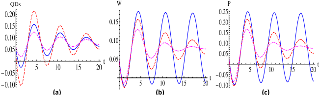
Figure 1: (Color online) Plot (a) shows the variation of all QDs with time ($t$) for single spin-$\frac{1}{2}$ atomic coherent state in the presence of QND noise with bath parameters $\gamma_{0}=0.1,\,\omega_{c}=100,$ squeezing parameters $r=0,\,a=0,$ and $\omega=1.0$ at temperature $T=1$, and $\alpha=\frac{\pi}{2},\,\beta=\frac{\pi}{3},\,\theta=\frac{\pi}{3},\,\phi=\frac{\pi}{4},$ in the units of $\hbar=k_{B}=1$. The smooth (blue) line, dashed (red) line and dot-dashed (magenta) line correspond to the $W$, $P$ and $Q$ functions, respectively; (b) and (c) show the variation of $W$ and $P$ functions with time for different temperatures $T=0,\,1$ and $2$ by smooth (blue) lines, dashed (red) lines and dot-dashed (magenta) lines, respectively.

III.2 Atomic coherent state in SGAD noise

Now, we take up a spin $j=\frac{1}{2}$, starting from an atomic coherent state, given by Eq. (19), evolving under a Squeezed Generalized Amplitude Damping (SGAD) channel, incorporating the effects of dissipation and bath squeezing and which includes the well known amplitude damping (AD) and generalized amplitude damping (GAD) channels as special cases. The Kraus operators of the SGAD channel are (SGAD, )

$$\begin{array}[]{lcl}E_{0}&=&\sqrt{p}\left[\begin{array}[]{cc}\sqrt{1-\lambda\left(t\right)}&0\\ 0&1\end{array}\right],\end{array}$$

$$\begin{array}[]{lcl}E_{1}&=&\sqrt{p}\left[\begin{array}[]{cc}0&0\\ \sqrt{\lambda\left(t\right)}&0\end{array}\right],\end{array}$$

$$\begin{array}[]{lcl}E_{2}&=&\sqrt{1-p}\left[\begin{array}[]{cc}\sqrt{1-\mu\left(t\right)}&0\\ 0&\sqrt{1-\nu\left(t\right)}\end{array}\right],\end{array}$$

$$\begin{array}[]{lcl}E_{3}&=&\sqrt{1-p}\left[\begin{array}[]{cc}0&\sqrt{\nu\left(t\right)}\\ \sqrt{\mu\left(t\right)}e^{-i\xi\left(t\right)}&0\end{array}\right],\end{array}$$ (24)

where $\lambda=\frac{1}{p}\left\{1-\left(1-p\right)\left[\mu+\nu\right]-\exp\left(-\gamma_{0}\left(2N+1\right)t\right)\right\},$ $\mu=\frac{2N+1}{2N\left(1-p\right)}\frac{\sinh^{2}\left(\gamma_{0}at/2\right)}{\sinh^{2}\left(\gamma_{0}\left(2N+1\right)t/2\right)}\exp\left(-\frac{\gamma_{0}}{2}\left(2N+1\right)t\right),$ and $\nu=\frac{N}{\left(1-p\right)\left(2N+1\right)}\left\{1-\exp\left(-\gamma_{0}\left(2N+1\right)t\right)\right\}.$ Here, for convenience we have omitted the time dependence in the argument of different time dependent parameters (e.g., $\lambda(t)$, $\mu(t)$, $\nu(t)$, etc.) in the Kraus operators of SGAD noise. Here, $\gamma_{0}$ is the spontaneous emission rate, $a=\sinh\left(2r\right)\left(2N_{th}+1\right),$ and $N=N_{th}\left\{\cosh^{2}\left(r\right)+\sinh^{2}\left(r\right)\right\}+\sinh^{2}\left(r\right),$ with $N_{th}=1/\left\{\exp\left(\hbar\omega/k_{B}T\right)-1\right\}$ being the Planck distribution. Here, $r$ and the bath squeezing angle ($\xi\left(t\right)$) are the bath squeezing parameters. The expression for $p$ in the above equations has an analytic, though complicated, expression, and we refer the reader to (SGAD, ) for details. Application of the above Kraus operators to the initial state results in

$$\begin{array}[]{lcl}\rho\left(t\right)&=&\overset{3}{\underset{i=0}{\Sigma}}E_{i}\left(t\right)\rho\left(0\right)E_{i}^{\dagger}\left(t\right).\end{array}$$

The state at time $t$ can be obtained as

$$\rho\left(t\right)=\left[\begin{array}[]{cc}\rho_{11}&\rho_{21}^{*}\\ \rho_{21}&1-\rho_{11}\end{array}\right],$$ (25)

where

$$\begin{array}[]{lcl}\rho_{11}&=&\frac{1}{2}\left\{1-\mu+\nu-p\left(\lambda-\mu+\nu\right)+\left(-1+\mu+\nu+p\left(\lambda-\mu-\nu\right)\right)\cos\alpha\right\},\end{array}$$

and

$$\begin{array}[]{lcl}\rho_{21}&=&\frac{1}{2}\sin\alpha\left\{\left(1-p\right)\sqrt{\mu\nu}e^{-i\left(\beta+\xi\right)}+p\sqrt{1-\lambda}e^{i\beta}+\left(1-p\right)\sqrt{\left(1-\mu\right)\left(1-\nu\right)}e^{i\beta}\right\}.\end{array}$$

Using this density matrix, we can calculate the evolution of the different QDs, in a manner similar to the previous example of evolution under QND channel, leading to

$$\begin{array}[]{lcl}W\left(\theta,\phi\right)&=&\frac{1}{4\pi}\left[1+\sqrt{3}\left\{-\mu+\nu-p\left(\lambda-\mu+\nu\right)+\left(-1+\mu+\nu+p\left(\lambda-\mu-\nu\right)\right)\cos\alpha\right\}\cos\theta\right.\\ &+&\sqrt{3}\left(\left\{p\sqrt{1-\lambda}+\left(1-p\right)\sqrt{\left(1-\mu\right)\left(1-\nu\right)}\right\}\cos\left(\beta+\phi\right)\right.\\ &+&\left.\left.\left(1-p\right)\sqrt{\mu\nu}\cos\left(\beta+\xi-\phi\right)\right)\sin\alpha\sin\theta\right];\end{array}$$ (26)

$$\begin{array}[]{lcl}P\left(\theta,\phi\right)&=&\frac{1}{4\pi}\left[1-3\left\{-\mu+\nu-p\left(\lambda-\mu+\nu\right)+\left(-1+\mu+\nu+p\left(\lambda-\mu-\nu\right)\right)\cos\alpha\right\}\cos\theta\right.\\ &+&3\left(\left\{p\sqrt{1-\lambda}+\left(1-p\right)\sqrt{\left(1-\mu\right)\left(1-\nu\right)}\right\}\cos\left(\beta+\phi\right)\right.\\ &+&\left.\left.\left(1-p\right)\sqrt{\mu\nu}\cos\left(\beta+\xi-\phi\right)\right)\sin\alpha\sin\theta\right];\end{array}$$ (27)

and

$$\begin{array}[]{lcl}Q\left(\theta,\phi\right)&=&\frac{1}{4\pi}\left[1-\left\{-\mu+\nu-p\left(\lambda-\mu+\nu\right)+\left(-1+\mu+\nu+p\left(\lambda-\mu-\nu\right)\right)\cos\alpha\right\}\cos\theta\right.\\ &+&\left(\left\{p\sqrt{1-\lambda}+\left(1-p\right)\sqrt{\left(1-\mu\right)\left(1-\nu\right)}\right\}\cos\left(\beta+\phi\right)\right.\\ &+&\left.\left.\left(1-p\right)\sqrt{\mu\nu}\cos\left(\beta+\xi-\phi\right)\right)\sin\alpha\sin\theta\right].\end{array}$$ (28)

The variation of all the QDs with time ($t$) for some specific values of the parameters is depicted in Fig. 2, which incorporates both temperature and squeezing. A comparison of the Figs. 2 a and 2 b brings out the effect of squeezing on the evolution of QDs. Further, it is easily observed that with the increase in $T$, the quantumness reduces. An important point to notice here, is that if we make the noise parameters zero, i.e., in the absence of noise, the different QDs given by Eqs. (26)-(28), reduce to a form exactly equal to the corresponding noiseless QDs obtained for QND evolutions (Eqs. (21)-(23)). Also, results for generalized amplitude damping channel can be obtained in the limit of vanishing squeezing, i.e., for $\mu\left(t\right)=0$ and $\lambda\left(t\right)=\nu\left(t\right)$, while corresponding results for QDs under evolution of an amplitude damping channel can be obtained by further setting $T=0$, and $p=1$. Further, it would be apt to mention here that the oscillatory nature of the QDs for an atomic coherent state evolving under QND noise is not seen here. This is consistent with the fact that the SGAD noise is dissipative in nature, involving decoherence along with dissipation.

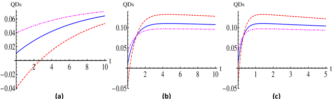
Figure 2: (Color online) The variation of all the distribution functions with time ($t$) is shown together for a single spin-$\frac{1}{2}$ atomic coherent state in the presence of the SGAD noise for zero bath squeezing angle in units of $\hbar=k_{B}=1$, with $\omega=1.0,\,\gamma_{0}=0.05,$ and $\alpha=\frac{\pi}{2},\,\beta=\frac{\pi}{3},\,\theta=\frac{\pi}{2},\,\phi=\frac{\pi}{3}.$ In (a) the variation with time is shown for temperature $T=3.0$ in the absence of squeezing parameter, i.e., $r=0$. In (b) the effect of the change in squeezing parameter for same temperature, i.e., $T=3.0$ is shown by using the squeezing parameter $r=1.0$, keeping all the other values as same as that used in (a). Further, in (c) keeping $r=1.0$ as in (b), the temperature is increased to $T=10$ to show the effect of variation in T. In (c) time is varied only up to $t=5$ to emphasize the effect of temperature. In all the three plots, smooth (blue), dashed (red) and dotted-dashed (magenta) lines correspond to the $W$, $P$ and $Q$ functions, respectively.

IV QDs for multiqubit systems undergoing QND and dissipative evolutions

Now, we wish to study the evolution of QDs for some interesting two and three qubit systems under general open system evolutions. We will also take up the well known $N$-qubit Dicke model. In each case, we study the nonclassicality exhibited by the system under consideration.

IV.1 Two qubits in the presence of QND noise

The density matrix for a system of two qubits in QND interaction with a squeezed thermal bath, as obtained in Ref. (2qubit-QND, ), is

$$\begin{array}[]{lcl}\rho_{\left\{i_{n},j_{n}\right\}}^{s}\left(t\right)&=&\exp\left[i\left\{\Theta_{\left\{i_{n},j_{n}\right\}}\left(t\right)-\Lambda_{\left\{i_{n},j_{n}\right\}}\left(t\right)\right\}\right]\exp\left[-\Gamma_{\left\{i_{n},j_{n}\right\}}^{sq}\left(t\right)\right]\rho^{s}\left(0\right),\end{array}$$ (29)

where $\rho_{\left\{i_{n},j_{n}\right\}}^{s}\left(t\right)$ is the two-qubit reduced density matrix obtained by tracing out the bath (reservoir) degrees of freedom and has the matrix representation $\left\langle i_{2},i_{1}\right|\rho^{s}\left(t\right)\left|j_{2},j_{1}\right\rangle$, and $\left\{i_{n},j_{n}\right\}$ stands for $i_{1},j_{1};i_{2},j_{2}$. In this model, the system-bath coupling is dependent upon the position of the qubit, resulting in the classification of the dynamics into two regimes: (a) Localized model, where the inter-qubit spacing is greater than or of the order of the length scale set by the bath, and (b) Collective model, where the qubits are close enough to experience the same bath (2qubit-QND, ). Here, for the sake of brevity, we will provide details of the localized model only. The terms $\Theta_{\left\{i_{n},j_{n}\right\}}\left(t\right)$, $\Lambda_{\left\{i_{n},j_{n}\right\}}\left(t\right)$ and $\Gamma_{\left\{i_{n},j_{n}\right\}}^{sq}\left(t\right)$ have different expressions in the localized and collective models. The superscript $sq$ indicates that the bath starts in a squeezed thermal initial state. For convenience, the two particle index in Eq. (29) is denoted by a single 4-level index in the following manner:

$$-\frac{1}{2},-\frac{1}{2}\equiv 0;\;-\frac{1}{2},\frac{1}{2}\equiv 1;\;\frac{1}{2},-\frac{1}{2}\equiv 2;\;\frac{1}{2},\frac{1}{2}\equiv 3.$$

All the sixteen terms, of the density matrix, can be analytically calculated for a given initial state $\rho^{s}\left(0\right)$. In the localized model, considered here, the density matrix is obtained using the symmetry of the density matrix $\rho^{s}\left(t\right)$, i.e., symmetries between the matrix elements and hermiticity of the density matrix, and the expressions of different terms in Eq. (29) (2qubit-QND, ). The elements

$$\rho_{32}^{s}\left(t\right)=\rho_{23}^{*s}\left(t\right)=\rho_{01}^{s}\left(t\right)=\rho_{10}^{*s}\left(t\right),$$

are obtained using

$$\begin{array}[]{lcl}\Theta_{32}\left(t\right)&=&\Theta_{01}\left(t\right)=-\Theta_{23}\left(t\right)=-\Theta_{10}\left(t\right)\\ &=&\intop_{0}^{\infty}d\omega I\left(\omega\right)S\left(\omega,t\right)\cos\omega t_{s},\end{array}$$

and

$$\begin{array}[]{lcl}\Lambda_{32}\left(t\right)&=&\Lambda_{01}\left(t\right)=-\Lambda_{23}\left(t\right)=-\Lambda_{10}\left(t\right)\\ &=&-\intop_{0}^{\infty}d\omega I\left(\omega\right)C\left(\omega,t\right)\sin\omega t_{s},\end{array}$$

where $I\left(\omega\right)$ is the bath spectral density. In the Ohmic case considered here, $I\left(\omega\right)=\frac{\gamma_{0}}{\pi}\omega e^{-\omega/\omega_{c}},$ where $\gamma_{0}$ and $\omega_{c}$ are bath parameters. We have $S\left(\omega,t\right)=\frac{\omega t-\sin\omega t}{\omega^{2}},$ $C\left(\omega,t\right)=\frac{1-\cos\omega t}{\omega^{2}},$ $\omega t_{s}\equiv k.r_{mn},$ where $r_{mn}$ is the inter-qubit spacing and $t_{s}$ is the transit time introduced for the purpose of expressing the coupling of the system to its bath in the frequency domain. The diagonal elements of the density matrix are

$$\rho_{aa}^{s}\left(t\right)=\rho_{aa}^{s}\left(0\right),{\rm\;where}\,a=0,1,2,3,$$

implying an unchanging population, a characteristic of QND evolution. Also,

$$\rho_{21}^{s}\left(t\right)=\rho_{12}^{*s}\left(t\right)=\rho_{12}^{s}\left(t\right),$$

$$\rho_{30}^{s}\left(t\right)=\rho_{03}^{*s}\left(t\right)=\rho_{03}^{s}\left(t\right),$$

i.e., these elements are purely real and for these $\Theta\left(t\right)=0=\Lambda\left(t\right).$ The remaining elements are

$$\rho_{31}^{s}\left(t\right)=\rho_{13}^{*s}\left(t\right)=\rho_{02}^{s}\left(t\right)=\rho_{20}^{*s}\left(t\right),$$

and for their calculation we need

$$\begin{array}[]{lcl}\Theta_{31}\left(t\right)&=&\Theta_{02}\left(t\right)=-\Theta_{13}\left(t\right)=-\Theta_{20}\left(t\right)\\ &=&\intop_{0}^{\infty}d\omega I\left(\omega\right)S\left(\omega,t\right)\cos\omega t_{s},\end{array}$$

and

$$\begin{array}[]{lcl}\Lambda_{31}\left(t\right)&=&\Lambda_{02}\left(t\right)=-\Lambda_{13}\left(t\right)=-\Lambda_{20}\left(t\right)\\ &=&\intop_{0}^{\infty}d\omega I\left(\omega\right)C\left(\omega,t\right)\sin\omega t_{s}.\end{array}$$

For the determination of all these elements of the density matrix at time $t$, we also need $\Gamma^{sq}\left(t\right)$ which have complex expressions and can be seen in (2qubit-QND, ). Once the density matrix at time $t$ is obtained, the corresponding QDs can be obtained from the prescription discussed above. However, getting analytic expressions for different QDs, here, is a cumbersome task; hence we will resort to numerically plotting them. Without loss of generality, we consider here our initial state to be such that all the sixteen elements of the density matrix at time $t=0$ are 0.25. The effect of QND interaction on different QDs obtained for this particular choice of initial state is shown in Fig. 3. As can be seen from the figure, both the $P$ and $W$ functions exhibit negative values, indicative of quantumness in the system, for some time after initiation of the evolution, before becoming positive, due to dephasing caused by the bath. As expected, the $P$ function is a stronger indicator of quantumness than the $W$ function, while the $Q$ function is always positive, by construction.

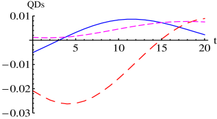
Figure 3: (Color online) The plot shows the variation of all the QDs with time for two qubits undergoing QND evolution with $\gamma_{0}=0.01,\,\omega_{c}=100,$ $k.r_{ab}=0.05,$ squeezing parameters $r=0.05,\,a=0,$ which implies zero squeezing angle, and temperature $T=2$ with $\theta_{1}=\frac{\pi}{3},\,\theta_{2}=\frac{\pi}{4},\,\phi_{1}=\pi,\,\phi_{2}=\frac{\pi}{3}$ in units of $\hbar=k_{B}=1$. The smooth (blue), large dashed (red), and small dashed (magenta) lines correspond to $W$, $P$ and $Q$ functions, respectively.

IV.2 Two qubits under dissipative evolution

Here, we study the evolution of QDs, for two qubit systems, undergoing dissipative evolution, first interacting with a vacuum bath, $T=0$ and zero bath squeezing, and then under the influence of a squeezed thermal bath, finite $T$ and bath squeezing. Here, we will make use of the results worked out in Ref. (squ-ther-bath, ).

IV.2.1 Vacuum bath

The density matrix, in the dressed state basis, can be used for calculating different QDs. We consider the initial state with one qubit in the excited state $\left|e_{1}\right\rangle$ and the other in the ground state $\left|g_{2}\right\rangle$, i.e., $\left|e_{1}\right\rangle\left|g_{2}\right\rangle$. The two-qubit reduced density matrix is given by

$$\begin{array}[]{lcl}\rho\left(t\right)&=&\left[\begin{array}[]{cccc}\rho_{ee}\left(t\right)&\rho_{es}\left(t\right)&\rho_{ea}\left(t\right)&\rho_{eg}\left(t\right)\\ \rho_{es}^{*}\left(t\right)&\rho_{ss}\left(t\right)&\rho_{sa}\left(t\right)&\rho_{sg}\left(t\right)\\ \rho_{ea}^{*}\left(t\right)&\rho_{sa}^{*}\left(t\right)&\rho_{aa}\left(t\right)&\rho_{ag}\left(t\right)\\ \rho_{eg}^{*}\left(t\right)&\rho_{sg}^{*}\left(t\right)&\rho_{ag}^{*}\left(t\right)&\rho_{gg}\left(t\right)\end{array}\right],\end{array}$$ (30)

where analytic expressions of all the elements of the density matrix in Eq. (30) can be seen from Eqs. (23)-(32) of Ref. (squ-ther-bath, ).

Here, we consider identical qubits. The dynamics involve collective coherent effects due to the multiqubit interaction, as well collective incoherent effects due to dissipative multiqubit interaction with the bath, and spontaneous emission. Analytic expressions of the corresponding QDs are very cumbersome, hence we resort to numerically studying the QDs for some parameters. Values of different parameters are as follows wavevector and mean frequency $k_{0}=\omega_{0}=1$, spontaneous emission rate $\Gamma_{j}=0.05$, and $\hat{\mu}\cdot\hat{r}_{ij}=0$, where $\hat{\mu}$ is equal to the unit vector along the atomic transition dipole moment and $\hat{r}_{ij}$ is the interatomic distance. Considering the initial state with $\rho_{ee}\left(0\right)=\rho_{gg}\left(0\right)=\rho_{es}\left(0\right)=\rho_{ea}\left(0\right)=\rho_{eg}\left(0\right)=\rho_{sg}\left(0\right)=\rho_{ag}\left(0\right)=0$, and $\rho_{ss}\left(0\right)=\rho_{aa}\left(0\right)=\rho_{sa}\left(0\right)=0.5$, the $W$, $P$, and $Q$ functions are calculated.

The variation of the different QDs is depicted in Figs. 4 and 5. Figs. 4 a and 4 b show the negative values of $W$ function and $P$ function for some and for all times, respectively. The $Q$ function exhibits a decaying pattern. These features are reinforced in the last plot of the figure, where all the QDs are plotted together. In Fig. 5, various QDs are plotted with respect to the inter-qubit distance. In the collective regime, $r_{12}\ll 1$, the QDs exhibit an oscillatory behavior, in consonance with the general behavior in this regime (squ-ther-bath, ). Also, for the chosen parameters, the $P$ function is always negative, while the $W$ function is negative for $t=1$, but becomes positive for a longer time $t=5$, due to the dissipative influence of the bath.

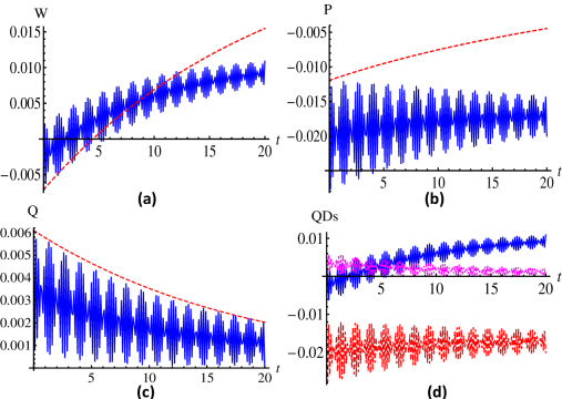
Figure 4: (Color online) The variation of the $W$, $P$, and $Q$ functions with time is shown in (a)-(c) for the two-qubit state, in the presence of vacuum bath, with $\theta_{1}=\frac{\pi}{8},\,\theta_{2}=\frac{\pi}{3},\,\phi_{1}=\frac{\pi}{4},\,\phi_{2}=\frac{\pi}{4}$ with the inter-qubit spacing $r_{12}=0.05$ (smooth blue line), and $r_{12}=2.0$ (red dashed line). In (d) all the QDs, varying with time, are plotted together with inter-qubit spacing $r_{12}=0.05$. Here the $P$ function is seen to be negative for all times shown, while the $W$ function is negative only for sometime, while the $Q$ function is always positive.

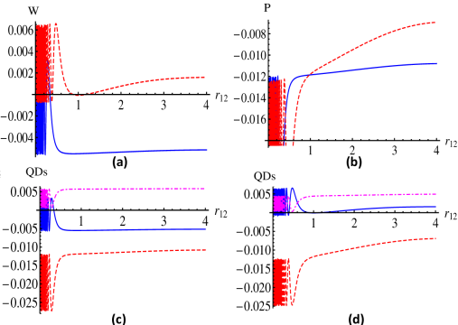
Figure 5: (Color online) (a) and (b) depict the $W$ and $P$ functions for the two qubit state, interacting with a vacuum bath, as a function of the inter-qubit spacing at $t=1$ (smooth blue line), and $t=5$ (red dashed line). In (c) and (d), $W$ (smooth blue line), $P$ (red dashed line) and $Q$ (magenta dot-dashed line) QDs are plotted together, depicting their variation with inter-qubit spacing at time $t=1$ and $t=5$, respectively. For all the plots $\theta_{1}=\frac{\pi}{8},\,\theta_{2}=\frac{\pi}{3},\,\phi_{1}=\frac{\pi}{4},\,{\rm and}\,\phi_{2}=\frac{\pi}{4}$.

IV.2.2 Squeezed thermal bath

Let us consider the evolution of same initial state, as in the presence of the vacuum bath at time $t=0$, but now evolving under the influence of a squeezed thermal bath with finite $T$ and $r$. Similar to the case of the vacuum bath, for certain values of the parameters in the density matrix, we can calculate different QDs. The elements of the density matrix in the presence of a squeezed thermal bath can be obtained as in Eqs. (33)-(40) in Ref. (squ-ther-bath, ). For simplicity, we take here the squeezing angle $\Phi=0$, and all other parameters are same as in the case of the vacuum bath, i.e., $k_{0}=\omega_{0}=1$, $\Gamma_{j}=0.05$, and $\hat{\mu}\cdot\hat{r}_{ij}=0$. From the density matrix of the evolved state, the various QDs can be obtained, which once more due to their cumbersome nature are studied numerically. The behavior of the different QDs is shown, for different parameters, in Figs. 6 and 7.

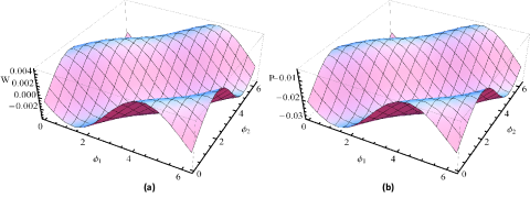
Figure 6: (Color online) $W$ and $P$ functions were able to detect the nonclassicality in the presence of squeezed thermal bath at time $t=2.0$ with $\theta_{1}=\frac{\pi}{4},\,\theta_{2}=\frac{\pi}{8}$, at temperature $T=1.0,$ squeezing parameter $r=0.5,$ and interatomic distance $kr_{12}=0.05$; all the remaining parameters are as mentioned above. The $Q$ function failed to detect nonclassicality. The $P$ function shows nonclassicality for all values of $\phi_{1}$ and $\phi_{2}$ as it is negative for all values of the chosen parameters.

In Figs. 6, three dimensional plots of $W$ and $P$ QDs are shown with respect to the azimuthal angles. The $P$ function exhibits negative values for all values of the parameters chosen, while the $W$ function does so for a restricted set of values. All these reiterate the quantumness of the state studied. From Fig. 7 a-b, the effect of finite bath squeezing $r$ and $T$ on the evolution of the QDs can be seen. In particular, with an increase in $T$, the QDs, both $P$ and $W$, which were earlier exhibiting negative values start becoming positive, a clear indicator of a quantum to classical transition. Fig. 7 c and d, showing the behavior of the QDs with respect to time and inter-qubit separations, are also along the expected lines. The nature of the QDs for small interqubit spacing, as seen here, is consistent with that of the same state subjected to dissipative interaction with a vacuum bath. Due to increase in temperature the oscillations observed in the QDs for small interqubit spacing, for the case of interaction with the vacuum bath in Fig. 5d, decreases in the present scenario of a squeezed thermal bath interaction and depicted in Fig. 7d. Further increase in temperature flattens the peak, observed for small inter-qubit spacing, in Fig. 7d.

IV.2.3 EPR singlet state in an amplitude damping (AD) channel

Now, we take an initially entangled two qubit, EPR singlet, state (EPR, ). The evolution of this state is studied assuming independent action of an amplitude damping (AD) channel on each qubit. Such a scenario could be envisaged in a quantum memory net with the qubits being its remote components, subject locally to the AD noise (eberly, ). Using Kraus operators of an AD channel

$$\begin{array}[]{lcl}E_{0}&=&\left[\begin{array}[]{cc}\sqrt{1-\lambda\left(t\right)}&0\\ 0&1\end{array}\right],\end{array}$$

$$\begin{array}[]{lcl}E_{1}&=&\left[\begin{array}[]{cc}0&0\\ \sqrt{\lambda\left(t\right)}&0\end{array}\right],\end{array}$$ (31)

where $\begin{array}[]{lcl}\lambda\left(t\right)&=&1-e^{-\gamma_{0}t},\end{array}$ where $\gamma_{0}$ is the spontaneous emission rate, and assuming that the two qubits, of the singlet, are independent and do not have any interaction, the Kraus operators for the action of AD channels, one on each spin, can be modeled as

$$\begin{array}[]{lcl}K_{1}&=&E_{0}\left(A\right)\otimes E_{0}\left(B\right),\\ K_{2}&=&E_{0}\left(A\right)\otimes E_{1}\left(B\right),\\ K_{3}&=&E_{1}\left(A\right)\otimes E_{0}\left(B\right),\\ K_{4}&=&E_{1}\left(A\right)\otimes E_{1}\left(B\right),\end{array}$$

where $A$ and $B$ stand for the first and second qubits (spins) comprising the singlet, respectively. From the form of Kraus operators (31) and assuming $\lambda_{A}=\lambda_{B}=\lambda$, we have

$$\begin{array}[]{lcl}K_{1}&=&\left[\begin{array}[]{cccc}1-\lambda&0&0&0\\ 0&\sqrt{1-\lambda}&0&0\\ 0&0&\sqrt{1-\lambda}&0\\ 0&0&0&1\end{array}\right],\end{array}$$

$$\begin{array}[]{lcl}K_{2}&=&\left[\begin{array}[]{cccc}0&0&0&0\\ \sqrt{\lambda\left(1-\lambda\right)}&0&0&0\\ 0&0&0&0\\ 0&0&\sqrt{\lambda}&0\end{array}\right],\end{array}$$

$$\begin{array}[]{lcl}K_{3}&=&\left[\begin{array}[]{cccc}0&0&0&0\\ 0&0&0&0\\ \sqrt{\lambda\left(1-\lambda\right)}&0&0&0\\ 0&\sqrt{\lambda}&0&0\end{array}\right],\end{array}$$

$$\begin{array}[]{lcl}K_{4}&=&\left[\begin{array}[]{cccc}0&0&0&0\\ 0&0&0&0\\ 0&0&0&0\\ \lambda&0&0&0\end{array}\right].\end{array}$$ (32)

The density matrix of the singlet state at time $t$, under the action of the above channel is

$$\begin{array}[]{lcl}\rho\left(t\right)&=&\overset{4}{\underset{i=1}{\Sigma}}K_{i}\left(t\right)\rho\left(0\right)K_{i}^{\dagger}\left(t\right),\end{array}$$

where $\rho\left(0\right)=\left|\phi\right\rangle\left\langle\phi\right|$, and $\begin{array}[]{lcl}\left|\phi\right\rangle&=&\frac{1}{\sqrt{2}}\left(\left|\frac{1}{2},-\frac{1}{2}\right\rangle-\left|-\frac{1}{2},\frac{1}{2}\right\rangle\right),\end{array}$ is the initial state at time $t=0$. Hence, at time $t$ the evolved density matrix is

$$\begin{array}[]{lcl}\rho\left(t\right)&=&\left[\begin{array}[]{cccc}0&0&0&0\\ 0&\frac{1}{2}\left(1-\lambda\right)&-\frac{1}{2}\left(1-\lambda\right)&0\\ 0&-\frac{1}{2}\left(1-\lambda\right)&\frac{1}{2}\left(1-\lambda\right)&0\\ 0&0&0&\lambda\end{array}\right].\end{array}$$ (33)

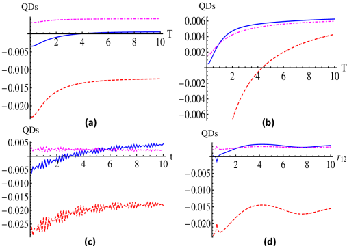
Figure 7: (Color online) Different QDs, evolving under the influence of a squeezed thermal bath, are plotted with $\theta_{1}=\frac{\pi}{4},\,\theta_{2}=\frac{\pi}{8},\,\phi_{1}=\frac{\pi}{6},\,\phi_{2}=\frac{\pi}{8}$, where smooth (blue), dashed (red) and dot-dashed (magenta) lines correspond to the $W$, $P$ and $Q$ functions, respectively. (a) and (b) are for temperature variation at time $t=2.0$ in two cases, (a) $r=0.5,\,kr_{12}=0.08$ (collective model), and (b) $r=-0.5,\,kr_{12}=1.5$ (localized model). In (c) all the QDs are plotted with respect to time with $T=1.0,\,r=0.1,\,kr_{12}=0.05$. And (d) shows the variation of all the QDs with $r_{12}$ for $T=1.0,\,t=2.0,\,r=0.5$.

On the evolved state, represented by the above density matrix, we may now apply the prescription for obtaining the QDs to yield compact analytical expressions of the various QDs. Specifically, the $W$ function is obtained as

$$\begin{array}[]{lcl}W\left(\theta_{1},\phi_{1},\theta_{2},\phi_{2}\right)&=&\frac{1}{16\pi^{2}}\left[\lambda\left\{1+3\cos\theta_{1}\cos\theta_{2}-\sqrt{3}\left(\cos\theta_{1}+\cos\theta_{2}\right)\right\}\right.\\ &+&\left.\left(1-\lambda\right)\left\{1-3\cos\theta_{1}\cos\theta_{2}-3\sin\theta_{1}\sin\theta_{2}\cos\left(\phi_{1}-\phi_{2}\right)\right\}\right],\end{array}$$ (34)

while the $P$ function is

$$\begin{array}[]{lcl}P\left(\theta_{1},\phi_{1},\theta_{2},\phi_{2}\right)&=&\frac{1}{16\pi^{2}}\left[\lambda\left\{1+9\cos\theta_{1}\cos\theta_{2}+3\left(\cos\theta_{1}+\cos\theta_{2}\right)\right\}\right.\\ &+&\left.\left(1-\lambda\right)\left\{1-9\cos\theta_{1}\cos\theta_{2}-9\sin\theta_{1}\sin\theta_{2}\cos\left(\phi_{1}-\phi_{2}\right)\right\}\right],\end{array}$$ (35)

and the $Q$ function is

$$\begin{array}[]{lcl}Q\left(\theta_{1},\phi_{1},\theta_{2},\phi_{2}\right)&=&\frac{1}{16\pi^{2}}\left[\lambda\left\{1+\cos\theta_{1}\cos\theta_{2}+\left(\cos\theta_{1}+\cos\theta_{2}\right)\right\}\right.\\ &+&\left.\left(1-\lambda\right)\left\{1-\cos\theta_{1}\cos\theta_{2}-\sin\theta_{1}\sin\theta_{2}\cos\left(\phi_{1}-\phi_{2}\right)\right\}\right].\end{array}$$ (36)

The QDs, reported here for an EPR pair (singlet state) evolving under AD channel exactly match with the corresponding noiseless results (agarwal, ; rama, ), by setting $\lambda=0$ in the above expressions. The variation of the different QDs with time is shown in Fig. 8. The $P$ and $W$ functions are found to show negative values for a long time, indicative of the perfect initial entanglement in the system, and finally become positive due to exposure to noise.

As all the QDs, in this case, are symmetric pairwise in $\left(\theta_{1}\leftrightarrow\theta_{2}\right)$ and $\left(\phi_{1}\leftrightarrow\phi_{2}\right)$, hence either or both of these exchanges would leave the expressions unchanged. For $\theta_{1}=-\theta_{2}=\frac{\pi}{2}$, and $\phi_{1}=\phi_{2}=0$, we observe the classically perfect anti-correlation of spins. We can also observe that for certain angles, viz. $\theta_{1}=\theta_{2}=\frac{\pi}{2}$, and $\phi_{1}-\phi_{2}=\frac{n\pi}{2},$ where $n$ is an odd integer, all the QDs become equal to $\frac{1}{\left(4\pi\right)^{2}}$, a result which remains unaffected by the presence or absence of noise. Hence, for these settings, the evolution of the QDs becomes noise independent.

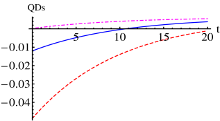
Figure 8: (Color online) The variation of all the QDs with time $t$ for EPR singlet state in the presence of AD channel with $\gamma_{0}=0.1$ and $\theta_{1}=\frac{\pi}{2},\theta_{2}=\frac{\pi}{2},\phi_{1}=\frac{\pi}{4},\phi_{2}=\frac{\pi}{3}$. Smooth (blue), dashed (red) and dot-dashed (magenta) lines are for $W$, $P$ and $Q$ functions, respectively.

IV.3 Three qubit QDs evolution in an AD channel

Three qubit entangled states can be classified into two classes (GHZ and W classes) of quantum states, such that a state of W (GHZ) class cannot be transformed to a state of GHZ (W) class by using LOCC (local operation and classical communication). Here, we study both GHZ (ghz, ) and W (w, ) classes of states. To simulate the effect of noise, we consider the scenario wherein the first qubit is affected by the AD channel. An arbitrary effect of noise on each subsystem could be thought of as more natural. The assumption of only one subsystem affected by amplitude damping noise is consistent with the effect of noise considered in, for example, various cryptrographic protocols (our-cryp and references therein), where it is commonly assumed that the qubits which travel through the channel are affected by noise while the channel noise does not affect the qubits to be teleported or not travelling through it.

IV.3.1 GHZ state in an amplitude damping (AD) channel

The GHZ (Greenberger–Horne–Zeilinger) state is a three qubit quantum state $\begin{array}[]{lcl}\left|GHZ\right\rangle&=&\frac{1}{\sqrt{2}}\left(\left|000\right\rangle+\left|111\right\rangle\right).\end{array}$ The first qubit of the state is acted upon by an amplitude damping (AD) channel while the remaining two qubits remain unaffected. The Kraus operators for AD channel for a single qubit state are as in Eq. (31). Here, assuming that the three qubits are independent of each other and do not have any interactions, the Kraus operators for the action of AD channel only on the first qubit, can be modeled as

$$\begin{array}[]{lcl}K_{1}&=&E_{0}\left(A\right)\otimes\mathbb{I}\left(B\right)\otimes\mathbb{I}\left(C\right),\\ K_{2}&=&E_{1}\left(A\right)\otimes\mathbb{I}\left(B\right)\otimes\mathbb{I}\left(C\right),\end{array}$$ (37)

where $E_{0}$ and $E_{1}$ are as in Eq. (31) and $\mathbb{I}$ is a $2\times 2$ identity matrix. Also, $A$, $B$ and $C$ stand for the first, second and third qubits of the GHZ state, respectively. Thus, the density matrix of the GHZ state at time $t$ in the amplitude damping channel is

$$\begin{array}[]{lcl}\rho\left(t\right)&=&\overset{2}{\underset{i=1}{\Sigma}}K_{i}\left(t\right)\rho\left(0\right)K_{i}^{\dagger}\left(t\right),\end{array}$$ (38)

where $\rho\left(0\right)=\left|GHZ\right\rangle\left\langle GHZ\right|,$ is the initial state at time $t=0$. Thus, at time $t$ the density matrix for the GHZ state evolving in the presence of the AD channel is

$$\begin{array}[]{lcl}\rho\left(t\right)&=&\frac{1}{2}\left[\begin{array}[]{cccccccc}\left(1-\lambda\right)&0&0&0&0&0&0&\sqrt{\left(1-\lambda\right)}\\ 0&0&0&0&0&0&0&0\\ 0&0&0&0&0&0&0&0\\ 0&0&0&0&0&0&0&0\\ 0&0&0&0&\lambda&0&0&0\\ 0&0&0&0&0&0&0&0\\ 0&0&0&0&0&0&0&0\\ \sqrt{\left(1-\lambda\right)}&0&0&0&0&0&0&1\end{array}\right].\end{array}$$ (39)

Analytical expressions can be obtained for the different QDs for the time evolved GHZ state described by Eq. (39).

Specifically, we obtain the $W$ function as

$$\begin{array}[]{lcl}W\left(\theta_{1},\phi_{1},\theta_{2},\phi_{2},\theta_{3},\phi_{3}\right)&=&\frac{1}{64\pi^{3}}\left[1-\sqrt{3}\lambda\cos\theta_{1}+3\cos\theta_{2}\cos\theta_{3}+3\left(1-\lambda\right)\cos\theta_{1}\left(\cos\theta_{2}+\cos\theta_{3}\right)\right.\\ &-&\left.3\sqrt{3}\left\{\lambda\cos\theta_{1}\cos\theta_{2}\cos\theta_{3}-\sqrt{\left(1-\lambda\right)}\sin\theta_{1}\sin\theta_{2}\sin\theta_{3}\cos\left(\phi_{1}+\phi_{2}+\phi_{3}\right)\right\}\right],\end{array}$$ (40)

while the $P$ function is

$$\begin{array}[]{lcl}P\left(\theta_{1},\phi_{1},\theta_{2},\phi_{2},\theta_{3},\phi_{3}\right)&=&\frac{1}{64\pi^{3}}\left[1+3\lambda\cos\theta_{1}+9\cos\theta_{2}\cos\theta_{3}+9\left(1-\lambda\right)\cos\theta_{1}\left(\cos\theta_{2}+\cos\theta_{3}\right)\right.\\ &+&\left.27\left\{\lambda\cos\theta_{1}\cos\theta_{2}\cos\theta_{3}-\sqrt{\left(1-\lambda\right)}\sin\theta_{1}\sin\theta_{2}\sin\theta_{3}\cos\left(\phi_{1}+\phi_{2}+\phi_{3}\right)\right\}\right],\end{array}$$ (41)

and the $Q$ function is

$$\begin{array}[]{lcl}Q\left(\theta_{1},\phi_{1},\theta_{2},\phi_{2},\theta_{3},\phi_{3}\right)&=&\frac{1}{64\pi^{3}}\left[1+\lambda\cos\theta_{1}+\cos\theta_{2}\cos\theta_{3}+\left(1-\lambda\right)\cos\theta_{1}\left(\cos\theta_{2}+\cos\theta_{3}\right)\right.\\ &+&\left.\lambda\cos\theta_{1}\cos\theta_{2}\cos\theta_{3}-\sqrt{\left(1-\lambda\right)}\sin\theta_{1}\sin\theta_{2}\sin\theta_{3}\cos\left(\phi_{1}+\phi_{2}+\phi_{3}\right)\right].\end{array}$$ (42)

The variation of the different QDs, as in Eqs. (40)-(42), with time is depicted, for a particular choice of the parameters, in Fig. 9a. The $W$ and $P$ functions exhibit negative values (nonclassical character) for the times shown, which could be attributed to the initial entanglement in the state. Further, for the sake of generality, we depict in Fig. 9b the scenario wherein all three qubits are affected by the generalized amplitude damping noise SGAD , which can be obtained from Eq. (24) by setting the bath squeezing parameters to zero. All three qubits are subjected to different temperatures corresponding to independent environment for each qubit, and simulates the scenario where each qubit travels through an independent channel. It can be observed that the nonclassicality indicated by the negativity of $W$ and $P$ functions at $t=0$ decays more rapidly when the last two qubits are subjected to finite temperature noises.

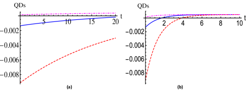
Figure 9: (Color online) The variation of all QDs with time for the GHZ state when acted upon by (a) an AD noise on the first qubit and (b) a generalized amplitude damping noise on each qubit, with $\gamma_{0}=0.1$ and $\theta_{1}=\frac{\pi}{2},\,\theta_{2}=\frac{\pi}{2},\,\theta_{3}=\frac{\pi}{2},\,\phi_{1}=\frac{\pi}{4},\,\phi_{2}=\frac{\pi}{3},\,\phi_{3}=\frac{\pi}{6}$. In (b) different QDs are shown for $\omega=1.0$ with the first, second and third qubits subjected to generalized amplitude damping noise at $T=0$, 1 and 2, respectively. In both the plots smooth (blue), dashed (red) and dot-dashed (magenta) lines are for the $W$, $P$ and $Q$ functions, respectively.

IV.3.2 W state in an amplitude damping (AD) channel

For our second example of QDs of three qubit states, we take up the W state $\begin{array}[]{lcl}\left|W\right\rangle&=&\frac{1}{\sqrt{3}}\left(\left|001\right\rangle+\left|010\right\rangle+\left|100\right\rangle\right).\end{array}$ As before, we consider the evolution where only the first qubit of the state is acted upon by an AD channel. The Kraus operators, describing the evolution are given by Eq. (37). Here, as in the case of GHZ or EPR states, assuming that the three qubits are independent of each other and do not have any interactions, the density matrix of the evolved state is, as in the last case, given by Eq. (38), where $\rho\left(0\right)=\left|W\right\rangle\left\langle W\right|,$ is the initial state at time $t=0$. Hence, at time $t$, the W state evolves, in the presence of the AD channel, to

$$\begin{array}[]{lcl}\rho\left(t\right)&=&\frac{1}{3}\left[\begin{array}[]{cccccccc}0&0&0&0&0&0&0&0\\ 0&\left(1-\lambda\right)&\left(1-\lambda\right)&0&\sqrt{\left(1-\lambda\right)}&0&0&0\\ 0&\left(1-\lambda\right)&\left(1-\lambda\right)&0&\sqrt{\left(1-\lambda\right)}&0&0&0\\ 0&0&0&0&0&0&0&0\\ 0&\sqrt{\left(1-\lambda\right)}&\sqrt{\left(1-\lambda\right)}&0&1&0&0&0\\ 0&0&0&0&0&\lambda&\lambda&0\\ 0&0&0&0&0&\lambda&\lambda&0\\ 0&0&0&0&0&0&0&0\end{array}\right].\end{array}$$ (43)

In this case, again, making use of Eq. (43), analytical forms of the different QDs can be obtained as follows

$$\begin{array}[]{lcl}W\left(\theta_{1},\phi_{1},\theta_{2},\phi_{2},\theta_{3},\phi_{3}\right)&=&\frac{1}{64\pi^{3}}\left[1-\left(\cos\theta_{1}\cos\theta_{2}+\cos\theta_{2}\cos\theta_{3}+\cos\theta_{1}\cos\theta_{3}\right)+\frac{\sqrt{3}}{3}\left(\cos\theta_{1}+\cos\theta_{2}+\cos\theta_{3}\right)\right.\\ &-&3\sqrt{3}\cos\theta_{1}\cos\theta_{2}\cos\theta_{3}+2\left(1+\sqrt{3}\cos\theta_{1}\right)\sin\theta_{2}\sin\theta_{3}\cos\left(\phi_{2}-\phi_{3}\right)\\ &+&2\sqrt{\left(1-\lambda\right)}\left\{\left(1+\sqrt{3}\cos\theta_{2}\right)\sin\theta_{1}\sin\theta_{3}\cos\left(\phi_{1}-\phi_{3}\right)\right.\\ &+&\left.\left(1+\sqrt{3}\cos\theta_{3}\right)\sin\theta_{1}\sin\theta_{2}\cos\left(\phi_{1}-\phi_{2}\right)\right\}\\ &+&\left.4\sqrt{3}\lambda\cos\theta_{1}\left\{-\frac{1}{3}+\cos\theta_{2}\cos\theta_{3}-\sin\theta_{2}\sin\theta_{3}\cos\left(\phi_{2}-\phi_{3}\right)\right\}\right],\end{array}$$ (44)

$$\begin{array}[]{lcl}P\left(\theta_{1},\phi_{1},\theta_{2},\phi_{2},\theta_{3},\phi_{3}\right)&=&\frac{1}{64\pi^{3}}\left[1-3\left(\cos\theta_{1}\cos\theta_{2}+\cos\theta_{2}\cos\theta_{3}+\cos\theta_{1}\cos\theta_{3}\right)-\left(\cos\theta_{1}+\cos\theta_{2}+\cos\theta_{3}\right)\right.\\ &+&27\cos\theta_{1}\cos\theta_{2}\cos\theta_{3}+6\left(1-3\cos\theta_{1}\right)\sin\theta_{2}\sin\theta_{3}\cos\left(\phi_{2}-\phi_{3}\right)\\ &+&6\sqrt{\left(1-\lambda\right)}\left\{\left(1-3\cos\theta_{2}\right)\sin\theta_{1}\sin\theta_{3}\cos\left(\phi_{1}-\phi_{3}\right)\right.\\ &+&\left.\left(1-3\cos\theta_{3}\right)\sin\theta_{1}\sin\theta_{2}\cos\left(\phi_{1}-\phi_{2}\right)\right\}\\ &+&\left.4\lambda\cos\theta_{1}\left\{1-9\cos\theta_{2}\cos\theta_{3}+9\sin\theta_{2}\sin\theta_{3}\cos\left(\phi_{2}-\phi_{3}\right)\right\}\right],\end{array}$$ (45)

and

$$\begin{array}[]{lcl}Q\left(\theta_{1},\phi_{1},\theta_{2},\phi_{2},\theta_{3},\phi_{3}\right)&=&\frac{1}{192\pi^{3}}\left[3-\left(\cos\theta_{1}\cos\theta_{2}+\cos\theta_{2}\cos\theta_{3}+\cos\theta_{1}\cos\theta_{3}\right)-\left(\cos\theta_{1}+\cos\theta_{2}+\cos\theta_{3}\right)\right.\\ &+&3\cos\theta_{1}\cos\theta_{2}\cos\theta_{3}+4\sin\frac{\theta_{1}^{2}}{2}\sin\theta_{2}\sin\theta_{3}\cos\left(\phi_{2}-\phi_{3}\right)\\ &+&4\sqrt{\left(1-\lambda\right)}\left\{\sin\theta_{1}\sin\frac{\theta_{2}^{2}}{2}\sin\theta_{3}\cos\left(\phi_{1}-\phi_{3}\right)+\sin\theta_{1}\sin\theta_{2}\sin\frac{\theta_{3}^{2}}{2}\cos\left(\phi_{1}-\phi_{2}\right)\right\}\\ &+&\left.4\lambda\cos\theta_{1}\left\{1-\cos\theta_{2}\cos\theta_{3}+\sin\theta_{2}\sin\theta_{3}\cos\left(\phi_{2}-\phi_{3}\right)\right\}\right].\end{array}$$ (46)

The variation of the QDs with time is shown in Fig. 10a for a particular choice of the parameters. Here, the $P$ function exhibits negative values for the times shown, but in contrast to the GHZ case, the $W$ function is found to be positive. Thus, the signature of quantumness (nonclassicality) of the state is identified by $P$ function, but $W$ function fails to detect the same. Similar to the QDs of GHZ state in the presence of generalized amplitude damping noise, a decrease in the nonclassicality of W state with time can be observed due to the effect of noise on the last two qubits at non-zero temperatures (cf. Fig. 10b).

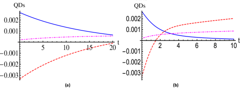
Figure 10: (Color online) (a) Variation of QDs with time for the W state in the presence of an AD channel, acting only upon the first qubit, with $\gamma_{0}=0.1$ and $\theta_{1}=\frac{\pi}{4},\,\theta_{2}=\frac{\pi}{6},\,\theta_{3}=\frac{\pi}{3},\,\phi_{1}=\frac{\pi}{8},\,\phi_{2}=\frac{\pi}{4},\,\phi_{3}=\frac{\pi}{6}$. (b) QDs for W state, when all the qubits are subjected to generalized amplitude damping noise, with $\omega=1.0$ and $T=0$, 1 and 2 for the first, second and third qubits, respectively. The remaining values of parameters in (b) are as in (a). Smooth (blue), dashed (red) and dot-dashed (magenta) lines correspond to $W$ function, $P$ function and $Q$ function, respectively.

IV.4 $N$ qubit Dicke Model

We conclude our discussion of QDs for two-level systems (qubits) with the Dicke model. The interaction of a collection of identical two-level atoms with a single mode of quantized field is the Dicke model (dicke, ; tacum, ) and is the multi-atom generalization of the Jaynes-Cummings model. The Hamiltonian for the Dicke model is given as

$$H=\omega\left(a^{\dagger}a+\Sigma_{z}^{c}\right)+g\left(a\Sigma_{+}^{c}+a^{\dagger}\Sigma_{-}^{c}\right).$$ (47)

Here, $\omega$ is the resonant atomic frequency, $g$ is the coupling constant, $a$ ($a^{\dagger}$) is the annihilation (creation) operator for the radiation field, and $\Sigma_{\pm}^{c}=\overset{N}{\underset{j=1}{\sum}}{\sigma^{\left(j\right)}}_{\pm},$ and $\Sigma_{z}^{c}=\frac{1}{2}\overset{N}{\underset{j=1}{\sum}}{\sigma^{\left(j\right)}}_{z},$ where $N$ is the number of atoms considered. Also, the symbol $c$ in the superscript stands for collective. A generalization of this model, dynamics of a collection of atoms interacting with a squeezed radiation field, was made in (AgPu, ). The Dicke model has analytical solutions in two regimes: weak and strong field regimes, which corresponds to average photon number being much smaller or greater than the number of atoms, respectively.

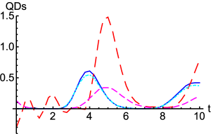
Figure 11: (Color online) Variation of all QDs with time for the $N=4$ atoms Dicke model with $\theta=\frac{\pi}{3},$ and $\phi=\frac{\pi}{2}.$ Smooth (blue), large dashed (red), small dashed (magenta) and dot-dashed (cyan) lines are for $W$ function, $P$ function, $Q$ function, and $F$ function, respectively. The four atom case is equivalent to the spin-2 case and consequently different values of the $W$ and $F$ functions can be observed.

We discuss, here, only the second case in the presence of strong initial field (DM, ), i.e., $\bar{n}\gg N$, where $\bar{n}$ is the average number of photons in the initial coherent field. In the dissipative case, modeling the microwave region of zero temperature dissipative cavity quantum electrodynamics, restricting ourselves to the condition $\frac{\gamma}{g}\ll\sqrt{\bar{n}}$, the master equation in Fock basis is

$$\begin{array}[]{lcl}\dot{\rho}_{nm}&=&-2ig\left(\Sigma_{x}^{c}\sqrt{n_{N}}\rho_{nm}-\rho_{nm}\sqrt{m_{N}}\Sigma_{x}^{c}\right)+\frac{\gamma}{2}\left(2a\rho a^{\dagger}-a^{\dagger}a\rho-\rho a^{\dagger}a\right)_{nm},\end{array}$$ (48)

where $n_{N}=n+\frac{1}{2}-\frac{N}{2}$, and $\gamma$ is the cavity decay constant. This master equation takes a simple form in the dressed atomic basis, in which the atomic operator $\Sigma_{x}^{c}=\frac{1}{2}(\Sigma_{+}^{c}+\Sigma_{-}^{c})$ is diagonal

$$\Sigma_{x}^{c}\left|\tilde{q}\right\rangle=\lambda_{q}\left|\tilde{q}\right\rangle,$$

where $\lambda_{q}=q-\frac{N}{2},$ and $q=0,1,\ldots,N.$ These dressed atomic states can be expressed in terms of the bare atomic basis as $\left|\tilde{q}\right\rangle=\underset{q}{\sum}C_{qk}\left|k\right\rangle,$ where $C_{qk}=\left\langle k\left|\tilde{q}\right.\right\rangle=i^{q-k}d_{qk}^{N}\left(-\frac{\pi}{2}\right),$ and $d_{qk}^{N}\left(\theta\right)$ are Wigner $d$ functions. The bare atomic basis (Dicke states) is defined as

$$\Sigma_{z}^{c}\left|k\right\rangle=\left(k-\frac{N}{2}\right)\left|k\right\rangle,\,\,\,\,0\leq k\leq N,$$

where $k$ is the number of excited atoms.

Now, we consider the initial atoms-field density matrix

$$\rho\left(0\right)=\left|{\rm atin}\right\rangle\left\langle{\rm atin}\right|\otimes\left|\alpha\right\rangle\left\langle\alpha\right|,$$

where $\left|{\rm atin}\right\rangle$ is the initial atomic state, taken here to be ground state, i.e., none of the atoms are excited and $\left|\alpha\right\rangle$ denotes the initial strong coherent state of the field. The atomic density matrix, in the bare atomic basis, after tracing out the radiation field evolves as

$$\begin{array}[]{lcl}\rho_{kl}\left(t\right)&=&\underset{n}{\sum}\alpha_{k+n}\left(t\right)\alpha_{l+n}^{*}\left(t\right)\overset{N}{\underset{q,p=0}{\Sigma}}C_{kq}C_{lp}C_{0q}C_{0p}^{*}G_{pq}^{n+k,n+l}\left(t\right),\end{array}$$ (49)

where

$$G_{qp}^{n,m}\left(t\right)=\exp\left[-2igt\left(\lambda_{q}\sqrt{n_{N}}-\lambda_{p}\sqrt{m_{N}}\right)-\Theta_{qp}\left(t\right)\right],$$

and $\Theta_{qp}\left(t\right)=\bar{n}\left\{\left(1-e^{-\gamma t}\right)-\frac{\gamma}{\gamma^{\prime}}\left(1-e^{-\gamma^{\prime}t}\right)\right\}$, $\gamma^{\prime}=\gamma+\frac{ig\left(\lambda_{q}-\lambda_{p}\right)}{\sqrt{\bar{n}\left(t\right)-\frac{N}{2}+\frac{1}{2}}}$ and $\alpha_{n}\left(t\right)=e^{-\bar{n}\left(t\right)/2}\frac{\bar{n}\left(t\right)^{n/2}}{\sqrt{n!}},$ with $\bar{n}\left(t\right)=\bar{n}e^{-\gamma t}.$

The evolution of all the QDs can be obtained for the Dicke model in the dissipative case using Eq. (49). Here, we consider the $N=4$ atoms Dicke model in a strong initial field with average photon number 30. Further, we take $\frac{\gamma}{g}=10^{-2},$ and coupling constant as 0.1. To achieve consistence with the notations used in this article, we have used $j=\frac{N}{2}$, and $m,\,m^{\prime}=-j,\ldots,j$. The multipole operators required to calculate the QDs are equivalent to spin-2 multipole operators and can be seen in Appendix. In Fig. 11, variation of the various QDs, as they evolve with time, is depicted. The $P$ function exhibits negative values at some early times, indicative of the quintessence of quantumness in the system, but eventually becomes positive due to dissipative effects. Different values of the $W$ and $F$ QDs are observed at some time intervals, consistent with the observation that the four atom case is equivalent to the spin-2 case. For this specific choice of parameters and restricting ourselves to the computational accuracy of the numerical method adopted here, we did not observe any signature of nonclassicality via $W$ function. However, $W$ function can witness the nonclassical characteristics present in the Dicke model for other values of $\theta$ and $\phi$. This point will be clearly illustrated in Fig. 13 d, where we show positive values of nonclassical volume (which is obtained by integrating the modulus of $W$ function over all possible values of $\theta$ and $\phi$) for the Dicke model. These positive values of nonclassical volume imply negative values of $W$ function for some values of $\theta$ and $\phi$ (cf. (Eq. 54)).

V QDs for a spin-1 state

Now, we extend the discussion of spin QDs from spin-$\frac{1}{2}$ to spin-1 states. For a spin-1 pure state (blum, )

$$\left|\chi\right\rangle=a_{+}\left|+1\right\rangle+a_{0}\left|0\right\rangle+a_{-}\left|-1\right\rangle,$$

QDs can be constructed using appropriate multipole operators and spherical harmonics. A few relevant multipole operators are $T_{00}=\frac{1}{\sqrt{3}}\left[\begin{array}[]{ccc}1&0&0\\ 0&1&0\\ 0&0&1\end{array}\right],$ $T_{11}=\frac{1}{\sqrt{2}}\left[\begin{array}[]{ccc}0&-1&0\\ 0&0&-1\\ 0&0&0\end{array}\right],$ $T_{10}=\frac{1}{\sqrt{2}}\left[\begin{array}[]{ccc}1&0&0\\ 0&0&0\\ 0&0&-1\end{array}\right],$ $T_{22}=\left[\begin{array}[]{ccc}0&0&1\\ 0&0&0\\ 0&0&0\end{array}\right],$ $T_{21}=\frac{1}{\sqrt{2}}\left[\begin{array}[]{ccc}0&-1&0\\ 0&0&1\\ 0&0&0\end{array}\right],$ and $T_{20}=\frac{1}{\sqrt{6}}\left[\begin{array}[]{ccc}1&0&0\\ 0&-2&0\\ 0&0&1\end{array}\right].$ All other multipole operators can be obtained from these operators. The analytical expressions of the different QDs are obtained as

$$\begin{array}[]{lcl}W\left(\theta,\phi\right)&=&\frac{1}{16\pi}\left[4-\sqrt{10}+3\sqrt{10}\left(\cos^{2}\theta+\left|a_{0}\right|^{2}-3\left|a_{0}\right|^{2}\cos^{2}\theta\right)+6\sqrt{2}\left(\left|a_{+}\right|^{2}-\left|a_{-}\right|^{2}\right)\cos\theta\right.\\ &+&\left.\left(6a_{0}\sin\theta\left\{a_{+}^{*}\exp(-i\phi)\left(1+\sqrt{5}\cos\theta\right)+a_{-}^{*}\exp(i\phi)\left(1-\sqrt{5}\cos\theta\right)\right\}+3\sqrt{10}a_{+}a_{-}^{*}\sin^{2}\theta\exp(2i\phi)+{\rm c.c.}\right)\right],\end{array}$$ (50)

$$\begin{array}[]{lcl}P\left(\theta,\phi\right)&=&\frac{3}{8\pi}\left[-1+5\left(\cos^{2}\theta+\left|a_{0}\right|^{2}-3\left|a_{0}\right|^{2}\cos^{2}\theta\right)-2\left(\left|a_{+}\right|^{2}-\left|a_{-}\right|^{2}\right)\cos\theta\right.\\ &+&\left.\left(\sqrt{2}a_{0}\sin\theta\left\{a_{+}^{*}\exp(-i\phi)\left(1-5\cos\theta\right)+a_{-}^{*}\exp(i\phi)\left(1+5\cos\theta\right)\right\}+5a_{+}a_{-}^{*}\sin^{2}\theta\exp(2i\phi)+{\rm c.c.}\right)\right],\end{array}$$ (51)

$$\begin{array}[]{lcl}Q\left(\theta,\phi\right)&=&\frac{3}{16\pi}\left[1+\left(\cos^{2}\theta+\left|a_{0}\right|^{2}-3\left|a_{0}\right|^{2}\cos^{2}\theta\right)-2\left(\left|a_{+}\right|^{2}-\left|a_{-}\right|^{2}\right)\cos\theta\right.\\ &+&\left.\left(\sqrt{2}a_{0}\sin\theta\left\{a_{+}^{*}\exp(-i\phi)\left(1-\cos\theta\right)+a_{-}^{*}\exp(i\phi)\left(1+\cos\theta\right)\right\}+5a_{+}a_{-}^{*}\sin^{2}\theta\exp(2i\phi)+{\rm c.c.}\right)\right],\end{array}$$ (52)

and

$$\begin{array}[]{lcl}F\left(\theta,\phi\right)&=&\frac{3}{32\pi}\left[1+5\left(\cos^{2}\theta+\left|a_{0}\right|^{2}-3\left|a_{0}\right|^{2}\cos^{2}\theta\right)+4\sqrt{2}\left(\left|a_{+}\right|^{2}-\left|a_{-}\right|^{2}\right)\cos\theta\right.\\ &+&\left.\left(a_{0}\sin\theta\left\{a_{+}^{*}\exp(-i\phi)\left(4+5\sqrt{2}\cos\theta\right)+a_{-}^{*}\exp(i\phi)\left(4-5\sqrt{2}\cos\theta\right)\right\}+5a_{+}a_{-}^{*}\sin^{2}\theta\exp(2i\phi)+{\rm c.c.}\right)\right].\end{array}$$ (53)

In Fig. 12, we illustrate the behavior of the above QDs for $a_{+}=a_{0}=a_{-}=\frac{1}{\sqrt{3}}$. Here, we do not consider the effect of noise on the evolution of the QDs, a topic to which we will return back to, in the future. The purpose here, besides studying the quantumness in the system via the QDs, is to emphasize the nonequivalence, for the spin-1 case, of the $W$ and $F$ functions, in contrast to the spin-$\frac{1}{2}$ case. Fig. 12 depicts the behavior of the QDs with respect to $\theta$ and $\phi$, both of which show a symmetric behavior about the central point on the ordinate. The $P$, $W$ and $F$ functions exhibit negative values, indicative of the quantumness in the system, with the $P$ function being the most sensitive indicator, as expected. Also, the $F$ and $W$ functions are clearly distinct.

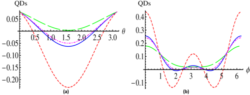
Figure 12: (Color online) Variation of all the QDs is shown for the spin-1 state with $a_{+}=a_{0}=a_{-}=\frac{1}{\sqrt{3}}.$ (a) shows $W$ (smooth blue line), $P$ (small dashed red line), $Q$ (large dashed green line), and $F$ (dot-dashed magenta line) functions with $\phi=\frac{2\pi}{3}.$ Similarly, (b) shows all the QDs for $\theta=\frac{\pi}{4}.$ Both (a) and (b) clearly bring out the point that $W$ and $F$ functions are not equal, in general, in contrast to the spin-$\frac{1}{2}$ cases.

VI Nonclassical volume

Till now, we have studied nonclassicality using negative values of the $W$ or $P$ function. Negative values of the QDs only provide a signature of nonclassicality, but they do not provide a quantitative measure of nonclassicality. There do exist some quantitative measures of nonclassicality, see for example, (with-adam-meas, ) for a review. One such measure is nonclassical volume introduced in (zyco, ). In this approach, the doubled volume of the integrated negative part of the $W$ function of a given quantum state is used as a quantitative measure of the quantumness (zyco, ). Using our knowledge of the $W$ functions for various systems, studied here, the nonclassical volume $\delta$, which is defined as

$$\delta=\int\left|W\left(\theta,\phi\right)\right|\sin\theta d\theta d\phi-1,$$ (54)

can be computed. It can be easily observed that a nonzero value of $\delta$ would imply the existence of nonclassicality, but this measure is not useful in measuring inherent nonclassicality in all quantum states. This is so because, the $W$ function is only a witness of nonclassicality (it does not provide a necessary condition). However, this measure of nonclassicality has been used in a number of optical systems, see for example, (with-adam, ; with-jay, ) and references therein.

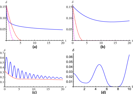
Figure 13: (Color online) The plots (a)-(d) depict the variation of the nonclassical volume in the presence of different noises. (a) The variation of the nonclassical volume with time is shown for the single spin-$\frac{1}{2}$ atomic coherent state in the presence of the QND noise with $\gamma_{0}=0.1,\,r=0,\,a=0,\,\omega_{c}=100,\,\omega=1.0,$ and $\alpha=\frac{\pi}{2},\,\beta=\frac{\pi}{3},$ in the units of $\hbar=k_{B}=1$, where the smooth (blue), dashed (red) and dot-dashed (magenta) lines correspond to different temperatures $T=0,\,1$ and $2$, respectively. (b) The variation of the nonclassical volume with time is shown for a single spin-$\frac{1}{2}$ atomic coherent state in a SGAD channel, where the smooth (blue) line corresponds to the variation in nonclassical volume in vacuum bath, i.e., at $T=0$ and squeezing parameters $r=\xi=0$ (amplitude damping channel); dashed (red) line corresponds to the variation in a channel with zero squeezing at $T=3$, i.e., generalized amplitude damping channel, and dot-dashed (magenta) line corresponds to the variation with squeezing $r=1,$ squeezing angle $\xi=0,$ and $T=3$. In all these cases $\alpha$ and $\beta$ have the same values as in (a). (c) The behavior of nonclassical volume with time is depicted in a vacuum bath for the state discussed in Section IV.2.1 with the inter-qubit spacing $r_{12}=0.05$ (smooth blue line), and $r_{12}=2.0$ (red dashed line). (d) The temporal behavior of nonclassical volume of the four atom Dicke model interacting with a strong input coherent field with average photon number 30, in the dissipative regime with $\frac{\gamma}{g}=10^{-2},$ and coupling constant as 0.1.

Here, we will illustrate the time evolution of $\delta$ for some of the spin-qubit systems, studied above. Specifically, Fig. 13 a and b show the variation of $\delta$ for two spin-$\frac{1}{2}$ systems, initially in an atomic coherent state under the influence of QND and SGAD channels, respectively. Fig. 13 c shows two spin-$\frac{1}{2}$ states in a two-qubit vacuum bath. The dashed and dot-dashed lines in Fig. 13 a and b, i.e., for atomic coherent state in QND with finite temperature and in SGAD with finite temperature and squeezing, exhibit the exponential reduction of nonclassical volume with time implying a quick transition from nonclassical to classical states, whereas the smooth lines in a and b (when temperature and squeezing parameters are taken to be zero) show that after an initial reduction, the nonclassical volume stabilizes over a reasonably large duration. Thus, nonclassicality does not get completely destroyed with time. A similar nature of time evolution of $\delta$ is also observed for the dashed line in Fig. 13 c (a two qubit state in a vacuum bath with relatively large inter-qubit spacing), whereas an oscillatory nature is observed for small inter-qubit spacing, depicted here by a smooth line. It should be noted that the smooth blue line in Fig. 13 b corresponds to the nonclassical volume for an atomic coherent state dissipatively interacting with a vacuum bath, i.e., at zero temperature and squeezing, while the $W$ function of the atomic coherent state, illustrated in Fig. 2, is for non-zero temperature and squeezing. At zero temperature, the nonclassicality present in the system is expected to survive for a relatively longer period of time. Further, the nonclassical volume is the overall contribution in nonclassicality from all values of $\theta$ and $\phi$. It is possible that the $W$ function shown for a particular value of $\theta$ and $\phi$, in the previous sections, may not exibit nonclassical behaviour at time $t$ whereas the other possible values provide a finite contribution to nonclassical volume, resulting in a nonvanishing $\delta$. Interestingly, in Fig. 13 d for the nonclassical volume of the Dicke model, we find that the amount of nonclassicality oscillates with time. This seems to arise from the weakness of the nonclassicality measure used here.

VII Conclusions

The nonclassical nature of all the systems studied here, of relevance to the fields of quantum optics and information, is illustrated via their quasiprobability distributions as a function of the time of evolution as well as various state or bath parameters. We also provide a quantitative idea of the amount of nonclassicality observed in some of the systems studied using a measure which essentially makes use of the $W$ function. These issues assume significance in questions related to quantum state engineering, where the central point is to have a clear understanding of coherences in the quantum mechanical system being used. Thus, it is essential to have an understanding over quantum to classical transitions, under ambient conditions. This is made possible by the present work, where a comprehensive analysis of QDs for spin-qubit systems is made under general open system effects, including both pure dephasing as well as dissipation, making it relevant from the perspective of experimental implementation. Along with the well known $W$, $P$ and $Q$ quasiprobability distributions, we also discuss the so called $F$ function and specify its relation to the $W$ function. We expect this work to have an impact on issues related to state reconstruction, in the presence of decoherence and dissipation. These quasiprobability distributions also play an important role in fundamental issues such as complementarity between number and phase distributions as well as for phase dispersion in atomic systems. It is interesting to note that in (victor, ), a connection was established between negative values of a particular quasiprobability and potential for quantum speed-up. The present study could be of use to probe this connection deeper.

Acknowledgement: A. P. and K.T. thank Department of Science and Technology (DST), India for support provided through the DST project No. SR/S2/LOP-0012/2010. SB thanks R. Srikanth for some useful discussions during the early stages of this work. We also thank Usha Devi for a number of helpful comments during various stages of this work.

Appendix: Multipole operators for Dicke model

Here, we collect the multipole operators used for the computation of QDs for the four qubit Dicke model in Sec. (IV.D).

$T_{00}=\frac{1}{\sqrt{5}}\left[\begin{array}[]{ccccc}1&0&0&0&0\\ 0&1&0&0&0\\ 0&0&1&0&0\\ 0&0&0&1&0\\ 0&0&0&0&1\end{array}\right],$ $T_{11}=\frac{1}{\sqrt{10}}\left[\begin{array}[]{ccccc}0&0&0&0&0\\ -\sqrt{2}&0&0&0&0\\ 0&-\sqrt{3}&0&0&0\\ 0&0&-\sqrt{3}&0&0\\ 0&0&0&-\sqrt{2}&0\end{array}\right],$ $T_{10}=\frac{1}{\sqrt{10}}\left[\begin{array}[]{ccccc}-2&0&0&0&0\\ 0&-1&0&0&0\\ 0&0&0&0&0\\ 0&0&0&1&0\\ 0&0&0&0&2\end{array}\right],$

$T_{22}=\frac{1}{\sqrt{7}}\left[\begin{array}[]{ccccc}0&0&0&0&0\\ 0&0&0&0&0\\ \sqrt{2}&0&0&0&0\\ 0&\sqrt{3}&0&0&0\\ 0&0&\sqrt{2}&0&0\end{array}\right],$ $T_{21}=\frac{1}{\sqrt{14}}\left[\begin{array}[]{ccccc}0&0&0&0&0\\ \sqrt{6}&0&0&0&0\\ 0&1&0&0&0\\ 0&0&-1&0&0\\ 0&0&0&-\sqrt{6}&0\end{array}\right],$ $T_{20}=\frac{1}{\sqrt{14}}\left[\begin{array}[]{ccccc}2&0&0&0&0\\ 0&-1&0&0&0\\ 0&0&-2&0&0\\ 0&0&0&1&0\\ 0&0&0&0&2\end{array}\right],$

$T_{33}=-\frac{1}{\sqrt{2}}\left[\begin{array}[]{ccccc}0&0&0&0&0\\ 0&0&0&0&0\\ 0&0&0&0&0\\ 1&0&0&0&0\\ 0&1&0&0&0\end{array}\right],$ $T_{32}=\frac{1}{\sqrt{2}}\left[\begin{array}[]{ccccc}0&0&0&0&0\\ 0&0&0&0&0\\ -1&0&0&0&0\\ 0&0&0&0&0\\ 0&0&1&0&0\end{array}\right],$ $T_{31}=\frac{1}{\sqrt{10}}\left[\begin{array}[]{ccccc}0&0&0&0&0\\ -\sqrt{3}&0&0&0&0\\ 0&\sqrt{2}&0&0&0\\ 0&0&\sqrt{2}&0&0\\ 0&0&0&-\sqrt{3}&0\end{array}\right],$

$T_{30}=\frac{1}{\sqrt{10}}\left[\begin{array}[]{ccccc}-1&0&0&0&0\\ 0&2&0&0&0\\ 0&0&0&0&0\\ 0&0&0&-2&0\\ 0&0&0&0&1\end{array}\right],$ $T_{44}=\left[\begin{array}[]{ccccc}0&0&0&0&0\\ 0&0&0&0&0\\ 0&0&0&0&0\\ 0&0&0&0&0\\ 1&0&0&0&0\end{array}\right],$ $T_{43}=\frac{1}{\sqrt{2}}\left[\begin{array}[]{ccccc}0&0&0&0&0\\ 0&0&0&0&0\\ 0&0&0&0&0\\ 1&0&0&0&0\\ 0&-1&0&0&0\end{array}\right],$

$T_{42}=\frac{1}{\sqrt{14}}\left[\begin{array}[]{ccccc}0&0&0&0&0\\ 0&0&0&0&0\\ \sqrt{3}&0&0&0&0\\ 0&-2\sqrt{2}&0&0&0\\ 0&0&\sqrt{3}&0&0\end{array}\right],$ $T_{41}=\frac{1}{\sqrt{14}}\left[\begin{array}[]{ccccc}0&0&0&0&0\\ 1&0&0&0&0\\ 0&-\sqrt{6}&0&0&0\\ 0&0&\sqrt{6}&0&0\\ 0&0&0&-1&0\end{array}\right],$ and $T_{40}=\frac{1}{\sqrt{70}}\left[\begin{array}[]{ccccc}1&0&0&0&0\\ 0&-4&0&0&0\\ 0&0&6&0&0\\ 0&0&0&-4&0\\ 0&0&0&0&1\end{array}\right].$

References

• (1) J. R. Klauder and E. C. G. Sudarshan, Fundamentals of Quantum Optics (Benjamin, New York 1968).
• (2) M. O. Scully and M. S. Zubairy, Quantum Optics (Cambridge University Press, Cambridge 1997).
• (3) W. P. Schleich, Quantum Optics in Phase Space (Wiley-VCH, Berlin 2001).
• (4) G. S. Agarwal, Quantum Optics (Cambridge University Press, Cambridge 2013).
• (5) R. R. Puri, Mathematical Methods of Quantum Optics (Springer, 2001).
• (6) A. B. Klimov and S. M. Chumakov, A Group-Theoretical Approach to Quantum Optics (Wiley-VCH, Weinheim 2009).
• (7) E. P. Wigner, Phys. Rev. 47, 749 (1932).
• (8) J. E. Moyal, Proc. Cambridge Philos. Soc. 45, 99 (1949).
• (9) M. Hillery, R. F. O’Connell, M. O. Scully and E. P. Wigner, Phys. Rep. 106, 121 (1984).
• (10) Y. S. Kim and M. E. Noz, Phase Space Picture of Quantum Mechanics (World Scientific, 1991).
• (11) A. Miranowicz, W. Leoński, and N. Imoto, Adv. Chem. Phys. 119, 155 (2001).
• (12) T. Opatrnỳ, A. Miranowicz, and J. Bajer, J. Mod. Opt. 43, 417 (1996).
• (13) R. J. Glauber, Phys. Rev. 131, 2766 (1963).
• (14) E. C. G. Sudarshan, Phys. Rev. Lett. 10, 277 (1963).
• (15) C. L. Mehta and E. C. G. Sudarshan, Phys. Rev. 138, B274 (1965).
• (16) Y. Kano, J. Phys. Soc. Japan 19, 1555 (1964).
• (17) K. Husimi, Proc. Phys. Math. Soc. Japan 22, 264 (1940).
• (18) J. Ryu, J. Lim, S. Hong and J. Lee, Phys. Rev. A 88, 052123 (2013).
• (19) A. Pathak, Elements of Quantum Computation and Quantum Communication (CRC Press, Boca Raton, USA (2013)).
• (20) M. Saffman, T. G. Walker and K. Molmer, Rev. Mod. Phys. 82, 2313 (2010).
• (21) A. Gaetan, et al., Nature Physics 5, 115 (2009).
• (22) R. H. Dicke, Phys. Rev. 93, 99 (1954).
• (23) J. P. Dowling, G. S. Agarwal and W. P. Schleich, Phys. Rev. A 49, 4101 (1994).
• (24) K. Wodkiewicz and J. H. Eberly, J. Opt. Soc. Am. B 2, 458 (1985).
• (25) M. Kitagawa and M. Ueda, Phys. Rev. Lett. 67, 1852 (1991).
• (26) V. P. Karassiov, Bull. Lebedev Phys. Inst. (Russian Academy of Science) N9, 34 (1999).
• (27) C. Zu, W.-B. Wang, L. He, W-.G. Zhang, C.-Y. Dai, F. Wang, and L.-M. Duan, Nature 514, 72 (2014).
• (28) C. Monroe, R. Raussendorf, A. Ruthven, K. R. Brown, P. Maunz, L.-M. Duan, and J. Kim, Phys. Rev. A 89, 022317 (2014).
• (29) J. A. Jones and M. Mosca, The Journal of Chemical Physics 109, 1648 (1998).
• (30) T. D. Ladd, J. R. Goldman, F. Yamaguchi, Y. Yamamoto, E. Abe, and K. M. Itoh, Phys. Rev. Lett. 89, 017901 (2002).
• (31) W. Harneit, Phys. Rev. A 65, 032322 (2002).
• (32) N. A. Gershenfeld, I. L. Chuang, Science 275, 350 (1997).
• (33) S. Sahling, G. Remenyi, C. Paulsen, P. Monceau, V. Saligrama, C. Marin, A. Revcolevschi, L. P. Regnault, S. Raymond, and J. E. Lorenzo, Nature Physics 11, 255 (2015).
• (34) R. L. Stratonovich, Sov. Phys. JETP 31, 1012 (1956).
• (35) A. B. Klimov and S. M. Chumakov, Revista Mexicana De Fisica 48, 317 (2002).
• (36) S. M. Chumakov, A. B. Klimov and K. B. Wolf, Phys. Rev. A 61, 034101 (2000).
• (37) W. K. Wootters, Ann. Phys. 176, 1 (1987).
• (38) A. Vourdas A, J. Phys. A: Math. Gen. 36, 5645 (2003).
• (39) S. Chaturvedi, et al., J. Phys. A: Math. Gen. 39 1405 (2006).
• (40) U. Leonhardt, Phys. Rev. A 53, 2998 (1996).
• (41) J. P. Paz, Phys. Rev. A 65 062311 (2002).
• (42) K. Blum, Density Matrix Theory and Applications (Plenum Press, New York 1996).
• (43) R. N. Zare, Angular Momentum: Understanding Spatial Aspects in Chemistry and Physics (John Wiley and Sons, 1988).
• (44) G. S. Agarwal, Phys. Rev. A 24, 2889 (1981); Phys. Rev. A 47, 4608 (1993).
• (45) L. Cohen and M. O. Scully, Found. Phys. 16, 295 (1986).
• (46) J. C. Varilly and J. M. Gracia-Bondia, Ann. of Phys. 190, 107 (1989).
• (47) F. T. Arecchi, E. Courtens, R. Gilmore and H. Thomas, Phys. Rev. A 6, 2211 (1972).
• (48) H. Margenau and R. N. Hill, Prog. Theor. Phys. 26, 722 (1961).
• (49) G. Ramachandran, A. R. Usha Devi, P. Devi and S. Sirsi, Found. of Phys. 26, 401 (1996); A. R. Usha Devi, Int. J. Mod. Phys. A 17, 2267 (2002).
• (50) W. H. Louisell, Quantum Statistical Properties of Radiation (John Wiley and Sons, 1973).
• (51) H.-P. Breuer and F. Petruccione, The Theory of Open Quantum Systems (Oxford University Press, 2002).
• (52) U. Weiss, Quantum Dissipative Systems (World Scientific, 2008).
• (53) S. Banerjee and R. Ghosh, Phys. Rev. E. 67, 056120 (2003).
• (54) Ş. K. Özdemir, A. Miranowicz, M. Koashi, and N. Imoto, Phys. Rev. A 64, 063818 (2001); Y. Makhlin, G. ${\rm Sch\ddot{o}n}$ and A. Shnirman, Rev. of Mod. Phys. 73, 357 (2001).
• (55) F. Verstraete, M. M. Wolf, and J. I. Cirac, Nature physics 5, 633 (2009).
• (56) S. Banerjee and R. Srikanth, Euro. Phys. J. D 46, 335 (2008).
• (57) S. Banerjee and R. Ghosh, J. Phys. A:Math. Theo. 40, 13735 (2007).
• (58) R. Srikanth and S. Banerjee, Phys. Rev. A 77, 012318 (2008).
• (59) M. Brune, E. Hagley, J. Dreyer, X. Maitre, et al., Phys. Rev. Lett. 77, 4887 (1996).
• (60) Q. A. Turchette, C. J. Myatt, B. E. King, C. A. Sackett, et al., Phys. Rev. A 62, 053807 (2000); C. J. Myatt, B. E. King, Q. A. Turchette, C. A. Sackett, et al., Nature 403, 269 (2000).
• (61) G. S. Agarwal, Phys. Rev. A 57, 671 (1998).
• (62) J. H. Shapiro and S. R. Shepard, Phys. Rev. A 43, 3795 (1991).
• (63) M. J. W. Hall, Quantum Opt. 3, 7 (1991).
• (64) G. S. Agarwal, S. Chaturvedi, K. Tara and V. Srinivasan, Phys. Rev. A 45, 4904 (1992); G. S. Agarwal and R. P. Singh, Phys. Lett. A 217, 215 (1996).
• (65) S. Banerjee, J. Ghosh, and R. Ghosh, Phys. Rev. A 75, 062106 (2007); S. Banerjee and R. Srikanth, Phys. Rev. A 76, 062109 (2007).
• (66) R. Srikanth and S. Banerjee, Eur. Phys. J. D 53, 217 (2009); S. Banerjee and R. Srikanth, Modern Phys. Lett. B 24, 2485 (2010); R. Srikanth and S. Banerjee, Phys. Lett. A 374, 3147 (2010).
• (67) J. ${\rm\check{Perina}}$, Quantum statistics of Linear and Nonlinear Optical Phenomena (Kluwer, Dordrecht-Boston, 1991).
• (68) A. Miranowicz, K. Bartkiewicz, A. Pathak, J. ${\rm\check{Perina}}$ Jr., Y.-N. Chen, and F. Nori, Phys. Rev A 91, 042309 (2015).
• (69) A. Kenfack and K. Zyczkowski, Jour. of Optics B: Quantum and Semiclassical Optics 6, 396 (2004).
• (70) D. A. Varshalovich, A. N. Moskalev and V. K. Khersonskii, Quantum Theory of Angular Momentum (World Scientific, Singapore, 1988).
• (71) S. Banerjee, V. Ravishankar and R. Srikanth, Euro. Phys. J. D 56, 277 (2010).
• (72) S. Banerjee, V. Ravishankar, R. Srikanth, Annals of Physics 325 (4), 816-834 (2010).
• (73) A. Einstein, B. Podolsky, and N. Rosen, Phys. Rev. 47, 777 (1935).
• (74) T. Yu and J. H. Eberly, Phys. Lett. A 283, 676 (2010).
• (75) D. M. Greenberger, M. A. Horne, and A. Zeilinger, in Bell’s Theorem, Quantum Theory and Conceptions of the Universe, edited by M. Kafatos, (Kluwer Academics, Dordrecht, Netherlands, 1989), pp. 73-76; D. Bouwmeester, J. W. Pan, M. Daniell, H. Weinfurter and A. Zeilinger, Phys. Rev. Lett. 82, 1345 (1999).
• (76) W. Dur, G. Vidal and J. I. Cirac, Phys. Rev. A 62, 062314 (2000).
• (77) K. Thapliyal and A. Pathak, Quant. Inform. Process. 14, 2599 (2015); V. Sharma, C, Shukla, S. Banerjee, and A. Pathak, Quant. Info. Process. DOI: 10.1007/s11128-015-1038-5 (2015).
• (78) M. Tavis and F. W. Cummings, Phys. Rev. 170, 379 (1968).
• (79) G. S. Agarwal and R. R. Puri, Phys. Rev. A 41, 3782 (1990).
• (80) C. Saavedra, A. B. Klimov, S. M. Chumakov and J. C. Retamal, Phys. Rev. A 58, 4078 (1998).
• (81) A. Miranowicz, M. Paprzycka, A. Pathak and F. Nori, Phys. Rev. A 89, 033812 (2014).
• (82) A. Pathak and J. Banerji, Phys. Lett. A 378, 117 (2014).
• (83) V. Veitch, C. Ferrie, D. Gross and J. Emerson, New Journal of Physics 14, 113011 (2012).