Adaptive Diffusion Schemes for Heterogeneous Networks

Abstract

In this paper, we deal with distributed estimation problems in diffusion networks with heterogeneous nodes, i.e., nodes that either implement different adaptive rules or differ in some other aspect such as the filter structure or length, or step size. Although such heterogeneous networks have been considered from the first works on diffusion networks, obtaining practical and robust schemes to adaptively adjust the combiners in different scenarios is still an open problem. In this paper, we study a diffusion strategy specially designed and suited to heterogeneous networks. Our approach is based on two key ingredients: 1) the adaptation and combination phases are completely decoupled, so that network nodes keep purely local estimations at all times; and 2) combiners are adapted to minimize estimates of the network mean-square-error. Our scheme is compared with the standard Adapt-then-Combine scheme and theoretically analyzed using energy conservation arguments. Several experiments involving networks with heterogeneous nodes show that the proposed decoupled Adapt-then-Combine approach with adaptive combiners outperforms other state-of-the-art techniques, becoming a competitive approach in these scenarios.

I Introduction

Over the last years, adaptive diffusion networks have become an attractive and robust approach to estimate a set of parameters of interest in a distributed manner (see, e.g., [1, 2, 3, 4, 5, 6, 7, 8, 9, 10, 11, 12, 13, 14, 15] and their references). Compared to other distributed schemes, such as incremental and consensus strategies, diffusion techniques present some advantages, e.g., they are more robust to link failures or they do not require the definition of a cyclic path that runs across the nodes as in incremental solutions [16]. Furthermore, they perform better than consensus techniques in terms of stability, convergence rate, and tracking ability [5]. For these reasons, adaptive diffusion networks are considered an efficient solution in applications such as target localization and tracking [4], environment monitoring [5], and spectrum sensing in mobile networks [4, 17], among others. Moreover, they are also suited to model complex behaviors exhibited by biological or socioeconomic networks [5].

Diffusion networks consist of a collection of connected nodes, linked according to a certain topology, that cooperate with each other through local interactions to solve a distributed inference or optimization problem in real time. Each node is able to extract information from its local measurements and combine it with the ones received from its neighbors [4, 5]. This is typically performed in two stages: adaptation and combination. The order in which these stages are performed leads to two possible schemes: Adapt-then-Combine (ATC) and Combine-then-Adapt (CTA) [1, 18]. In both cases, the adaptation and combination steps are interleaved with the communication of the intermediate estimates among neighbors. In general, it is assumed that this communication among the nodes is synchronous, though an analysis of asynchronous diffusion strategies is available in [19].

In this paper, we focus on heterogeneous diffusion networks. We refer as heterogeneous to networks whose nodes implement diverse update functions, i.e., they can differ in the filter length or structure, step sizes, or even in the implemented learning rule. This is different to other popular scenarios such as multitask or node-specific diffusion networks [23], where the heterogeneity is in the input that nodes receive or/and in the task they solve. Heterogeneous nodes are an interesting choice to improve the tracking performance of the network, or simply to achieve a better tradeoff between computational cost and convergence rate by updating the nodes with different algorithms. Thus, it is not surprising that such heterogeneous networks have been considered in the literature from the first works on diffusion networks. For instance, [4] and [5] already considered in the analysis of the ATC and CTA schemes the case of least-mean-squares (LMS) nodes with different step sizes, and [24] used the term heterogeneous to refer to informed and uninformed (i.e., without access to local measurements) nodes in a diffusion network.

Compared to multitask scenarios, experimental studies of this kind of networks have been quite limited up to now and we think that they deserve more attention. One possible explanation is that overall network performance can be very sensitive to an inappropriate selection of the network combiners. To illustrate this, Fig. 1 shows the performance of the ATC scheme of [18] for a fully-connected network of 5 nodes implementing LMS updates, using static combiners. In this example, four nodes have a common step size, whereas the last node uses a larger value that can provide faster convergence. As it can be seen, in this case the diffusion strategy actually degrades the convergence of the fast node and the steady-state performance of the slow ones with respect to the operation of these nodes in the non-cooperation case. This is due to the use of fixed combiners that ‘contaminate’ the estimation of the fast node during convergence, whereas during the steady-state regime slow nodes fuse their estimations with that coming from the fast node, resulting in larger rather than smaller estimation error.

Fast node

Slow node

Figure 1: Estimation error for two nodes of a fully-connected ATC network with 5 nodes. All nodes implement LMS rules, but node 1 (fast node) uses a larger step size than the rest of nodes.

This simple example illustrates the importance of adequate rules for setting and adjusting the combination parameters in heterogeneous networks. Indeed, combination weights play an essential role in the overall performance of the network. For instance, diffusion least-mean-squares (LMS) strategies can perform similarly to classical centralized solutions when the weights used to combine the neighbors estimates are optimally adjusted [4, 25, 26]. Initially, different static combination rules were proposed such as Uniform [27], Laplacian [28], Metropolis [28], and Relative Degree [29]. Some adaptive schemes for adjusting the combination weights (e.g., [25, 26, 30, 31]) have also been proposed in order to optimize the network performance under spatially varying signal-to-noise ratio (SNR). Although these adaptive rules can reduce the steady-state error with respect to static combiners, some experiments show a deterioration in the convergence behavior [31]. Consequently, some schemes propose the use of different rules for transitory and steady-state regimes and include mechanisms to switch from one rule to the other in an online manner [31, 32]. Since all these works are generally optimized assuming homogeneous nodes, an important challenge is related with the fact that all the above-mentioned combination rules result in degraded performance when used with heterogeneous networks, and there are presently no alternatives for dealing with such problem in a general case.

In this work, we focus on an alternative diffusion scheme especifically designed for heterogeneous networks. In our approach, firstly proposed in [33, 34], and which will be called Decoupled ATC (D-ATC), the adaptation phase is kept decoupled from the combination phase, i.e., the local estimation of each node is combined with the estimates received from its neighbors, as in standard ATC, but the resulting combined estimation is not fed back into the next adaptation step. This scheme presents a more clear separation between the adaptation and combination phases. As it will be shown later, this allows us to implement mean-square-error (MSE) based rules for the combination phase which offer an adequate behavior for heterogeneous networks. With these rules we obtain a significant improvement in convergence and steady-state performance with respect to previous approaches, both in tracking and stationary scenarios. In addition, our proposal seems to be a more natural scheme for asynchronous networks, which are receiving increasing attention [19].

This paper extends our previous works [33, 34] in different ways:

1. We analyze the mean behavior of our diffusion strategy and derive sufficient conditions for the network combiners that guarantee the mean stability of the algorithm.

2. Using energy conservation arguments [35], we derive closed-form expressions for the steady-state mean-square deviation (MSD) of the network and of its individual nodes in a non stationary environment.

3. We propose two new rules for adjusting the combination weights: One following a Least-Squares (LS) approach, in the same vein as the one introduced in [33, 34], and one based on the Affine Projection Algorithm (APA).

4. Finally, we include detailed simulation work, both for stationary and tracking scenarios, to illustrate the performance of the proposed schemes and to corroborate the theoretical results.

The paper is organized as follows. The general formulation of ATC diffusion strategies for heterogeneous networks, together with the introduction of adaptive combiners, is presented in Section II. In Section III, the Decoupled ATC strategy is proposed, and we theoretically analyze it in Section IV. APA and LS-based rules for adapting network combiners are derived in Section V. Experimental results are provided in Section VI, and we close the paper with our main conclusions and some possibilities for future works in Section VII.

I-A Notation

We use boldface lowercase letters to denote vectors and boldface uppercase letters to denote matrices. The superscript $T$ represents the transpose of a matrix or a vector. Depending on the context, ${\mathbf{0}}_{N}$ represents an $N\times N$ matrix or a length-$N$ column vector with all elements equal to zero, and $\mathds{1}_{N}$ is an all-ones column vector with length $N$. In addition, to simplify the arguments, we assume that all the variables are real. Table I summarizes the notation that is used throughout the paper.

TABLE I: Summary of the notation used in the paper

$N$	Number of nodes in the network
${\mathcal{N}}_{k}$	Neighborhood of node $k$, including itself
$N_{k}$	Cardinality of ${\mathcal{N}}_{k}$
${\bar{\cal N}}_{k}$	Neighborhood of node $k$, excluding itself
$\bar{N}_{k}$	Cardinality of ${\bar{\cal N}}_{k}$
$\bar{{\bf{b}}}_{k}$	Vector with the indexes of all nodes in ${\bar{\cal N}}_{k}$
$\bar{{{b}}}_{k}^{(m)}$	Index of the $m^{\text{th}}$ node connected to node $k$
${\mathbf{w}}_{\rm o}(n)$	Unknown time-varying parameter vector
${\bf{{\boldsymbol{\psi}}}}_{k}(n)$	Local estimate of ${\mathbf{w}}_{\rm o}(n)$ (based only
	on local data at node $k$)
${\bf{w}}_{k}(n)$	Combined estimate of ${\mathbf{w}}_{\rm o}(n)$ at node $k$
$\{d_{k}(n),{\mathbf{u}}_{k}(n)\}$	Local desired value and regression vector
	at node $k$
$v_{k}(n)$	Local noise at node $k$
$y_{k}(n)$	Local output of node $k$
$e_{k}(n)$	Local error of node $k$
$c_{\ell k}(n)$	Combination weight assigned by node $k$ to
	the estimate received from node $\ell\in{\cal N}_{k}$
${\bf{c}}_{k}(n)$	Vector with combination weights
	associated to node $k$
$\bar{{\bf{c}}}_{k}(n)$	Vector with the same entries of ${\bf{c}}_{k}(n)$,
	excluding $c_{kk}(n)$

II Heterogeneous diffusion networks with MSE-based adaptive combiners

II-A ATC and CTA diffusion strategies

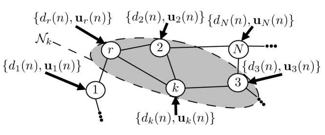
Figure 2: Example of diffusion network: At every time step $n$, each node $k$ takes a measurement $\{d_{k}(n),{\mathbf{u}}_{k}(n)\}$. In this example, the neighborhood of node $k$ is ${\mathcal{N}}_{k}=\{2,3,r,k\}$ and its cardinality is $N_{k}=4$.

Consider a collection of $N$ nodes connected according to a certain topology, as depicted in Fig. 2. Each node $k$ shares information with its neighbors and we denote this neighborhood of $k$, excluding the node itself, $\mathcal{\bar{N}}_{k}$, while $\mathcal{N}_{k}=\mathcal{\bar{N}}_{k}\cup\{k\}$. The network objective at every time instant $n$ is to obtain, in a distributed manner, the solution that minimizes a certain global cost function $J\left[{\mathbf{w}}(n)\right]$.

In this work, we consider that the global cost and the individual cost of each agent are the mean-square error (MSE). In particular, we consider a linear estimation setting: At every time instant $n$, each node $k$ has access to a scalar measurement $d_{k}(n)$ and a regression column vector ${\bf{u}}_{k}(n)$ of length $M$, both realizations of zero-mean random processes. We assume that these measurements are related via some unknown column vector ${\mathbf{w}}_{\rm o}(n)$ of length $M$ through a linear model

$$d_{k}(n)={\mathbf{u}}_{k}^{T}(n){\mathbf{w}}_{\rm o}(n)+v_{k}(n),$$ (1)

where $v_{k}(n)$ denotes measurement noise and is assumed to be a realization of a zero-mean white random process with power $\sigma_{v,k}^{2}$ and independent of all other variables across the network. The objective of the network is estimating the (possibly) time-varying parameter vector ${\mathbf{w}}_{\rm o}(n)$.

In standard ATC or CTA diffusion strategies, adaptation and combination phases are iterated to solve this estimation problem in an adaptive and distributed manner. In particular, the ATC scheme has the following two steps

$${\boldsymbol{\phi}}_{k}(n) =f_{k}({\mathbf{w}}_{k}(n-1),{\mathbf{u}}_{k}(n),d_{k}(n),\boldsymbol{\eta}_{k}),$$ (2)

$${\mathbf{w}}_{k}(n) =\sum_{\ell\in{\cal N}_{k}}c_{\ell k}(n){\boldsymbol{\phi}}_{\ell}(n),$$ (3)

where an intermediate estimation ${\boldsymbol{\phi}}_{k}(n)$ is calculated as a function of these elements: the previous estimation ${\mathbf{w}}_{k}(n-1)$, current local data $\{{\mathbf{u}}_{k}(n),d_{k}(n)\}$ and a state vector $\mathbf{\eta}_{k}$ that incorporates any other information needed for filter adaptation. Some typical choices for the adaptation stage (2) are least-mean-squares (LMS), normalized least-mean-squares (NLMS), Affine Projection Algorithm (APA) [35], etc. ${\boldsymbol{\phi}}_{k}(n)$ is then shared with the neighbors and combined by means of the coefficients $c_{\ell k}(n),\>\ell\in{\cal N}_{k}$, to calculate ${\mathbf{w}}_{k}(n)$.

Note that we assume that the update rules on (2) can be different among the nodes but all of them try to solve the same estimation task. This is complementary to other approaches such us multitask networks [36], where each node solves a different but related task.

II-B Adaptive combiners for heterogeneous networks

Different update rules to adapt the combiners in diffusion schemes have been proposed in the literature [25, 30, 26], all of them based in the approximated minimization of the network MSD (NMSD) defined as

$$\text{NMSD}(n)=\frac{1}{N}\sum_{k=1}^{N}\text{MSD}_{k}(n)=\frac{1}{N}\sum_{k=1}^{N}{\mathbb{E}}\{\left[{\mathbf{w}}_{\rm o}(n)-{\mathbf{w}}_{k}(n)\right]^{2}\},$$ (4)

where $\text{MSD}_{k}(n)$ is the mean-square deviation of each node $k$ in the network at iteration $n$.

However, the NMSD is very complicated to estimate as ${\mathbf{w}}_{\rm o}$ is unknown, and the available approximations [25, 30, 26] are only valid for the steady-state NMSD, $\text{NMSD}({\infty})=\lim_{n\rightarrow\infty}\text{NMSD}(n)$. Moreover, there is no approach in the literature that approximately minimizes (4) in heterogeneous networks, not even for the well-studied case of diffusion LMS networks with different step sizes in the nodes.

In this work, we follow a different approach. We propose an update rule driven by the online minimization of network MSE (NMSE), defined as

$$\text{NMSE}(n)=\frac{1}{N}\sum_{k=1}^{N}{\text{MSE}_{k}(n)}=\frac{1}{N}\sum_{k=1}^{N}{\mathbb{E}\{\check{e}^{2}_{k}(n)\}},$$ (5)

where $\check{e}_{k}(n)=d_{k}(n)-\check{y}_{k}(n)=d_{k}(n)-{\bf{u}}_{k}^{\scriptscriptstyle T}(n){\bf{w}}_{k}(n-1)$ represents the error at node $k$ using combined estimates available at that node, while $\check{y}_{k}(n)$ stands for the corresponding combined output.

It is well-known that for linear regression problems both criteria, MSD and MSE, are tightly related [35]. In our approach, $\text{MSE}_{k}(n)$ can be easily approximated during both the convergence and the steady-state phases, and whatever the kind of update implemented by each node of the network. In addition, other advantage of using the NMSE as the optimization criterion lies in the fact that its minimization can be tackled with well known algorithms to update the combination weights, including gradient-based or LS strategies. In this respect, while using the NMSD requires a model for the network performance to overcome the lack of knowledge of the optimum weight vector, minimization of the network MSE can be seen as a model-free approach.

Fig. 3 illustrates the performance of a standard ATC diffusion in a fully connected network with 5 LMS nodes. As in the example in Fig. 1, one node has a comparably larger step size than the other nodes. The scheme of [30], with adaptive combination weights (ATC ACW 2), is not able to exploit the fast convergence of the node with large step size. This is due to the lack of an accurate NMSD approximation during convergence. When the network combiners are adjusted using an LS criterion (ATC with LS combiner), the behavior of the network is similar to the use of static combiners, what made us wonder why the network did not fully exploit the best properties of the different nodes. When analyzing this problem in detail, we observed severe numerical problems due to the coupled nature of adaptation and combination stages in standard ATC, i.e., the feedback of the combined weights in the adaptation step causes almost perfect correlation among the weight estimations at all nodes, ill-conditioning the minimization of (5).

Figure 3: Estimation error for an ATC network with different combiners. It can be observed that state-of-the-art adaptive combination rules (in red) obtain a very good steady-state behaviour, much better that the ATC with LS combiners (black) because of the numerical problems of the latter.

In the next section, we propose a novel diffusion scheme that overcomes these numerical instabilities, permitting an effective use of NMSE-based adaptive combiners.

III Decoupled adapt-then-combine diffusion

Recently, we proposed a diffusion method [33, 34] that also iterates an adaptation and a combination phase. However, differently from standard ATC or CTA diffusion [4, 5], each node in our scheme preserves and adapts a purely local estimation ${\boldsymbol{\psi}}_{k}(n)$, which is then combined with the combined estimates, ${\mathbf{w}}_{\ell}(n-1)$, received from the neighboring nodes $\ell\in\mathcal{\bar{N}}_{k}$ at the previous iteration. Note that, although we have selected an ATC approach as the basis of our algorithm, it could be straightforwardly extended to CTA. Consequently, the proposed diffusion scheme can be written as follows

$${\boldsymbol{\psi}}_{k}(n) =f_{k}({\boldsymbol{\psi}}_{k}(n-1),{\mathbf{u}}_{k}(n),d_{k}(n),\boldsymbol{\eta}_{k}),$$ (6)

$${\mathbf{w}}_{k}(n) =c_{kk}(n){\boldsymbol{\psi}}_{k}(n)+\sum_{\ell\in\bar{\cal N}_{k}}c_{\ell k}(n){\mathbf{w}}_{\ell}(n-1).$$ (7)

with adaptive combiners $c_{\ell k}(n)$ selected to minimize (5).

In the adaptation phase (6), an updated local estimation ${\boldsymbol{\psi}}_{k}(n)$ is calculated as a function of the previous local estimation ${\boldsymbol{\psi}}_{k}(n-1)$, local data $\{d_{k}(n),{\mathbf{u}}_{k}(n)\}$ and a state vector $\boldsymbol{\eta}_{k}$. In the combination phase (7), each node calculates ${\mathbf{w}}_{k}(n)$ using time-varying combination coefficients $c_{\ell k}(n)$.

Two conditions are applied in the adaptation of $c_{\ell k}(n)$. Firstly, as most adaptive filtering schemes converge to unbiased estimations of the optimal solution in stationary scenarios, i.e., ${\mathbb{E}}\{{\mathbf{w}}_{\rm o}(n)-{\boldsymbol{\psi}}_{k}(n)\}\rightarrow 0$ as $n\rightarrow\infty$, we constrain all coefficients at each node to sum up to one, in order to keep combined weights estimations unbiased in steady state. In addition to this, to guarantee mean stability of our scheme, and in contrast with our previous work [33], we also impose non-negativity constraints on such combiners,

$$c_{\ell k}(n)\geq 0\text{, }\sum_{\ell\in\mathcal{N}_{k}}c_{\ell k}(n)=1,\forall k.$$ (8)

These conditions on combination coefficients have also been considered in other diffusion schemes available in the literature to guarantee certain stability properties.

The adaptation and combination stages on the proposed diffusion algorithm can be interpreted in the following way: with respect to the adaptation of local estimates ${\boldsymbol{\psi}}_{k}(n)$, each node could be considered as an isolated adaptive filter working independently from the rest of the network. Thus, it pursues the minimization of $\text{MSE}_{k}(n)$ using just its own regressors. During the combination phase, which includes the computation of combined weight estimators ${\mathbf{w}}_{k}(n)$ and the adaptation of the combiners, minimization of the network MSE is pursued.

We should emphasize that the most significant difference of (6) and (7) with respect to standard ATC is that the weight vector resulting from the combination is not fed back to the update of each individual filter. Even though under some circumstances this feedback can be beneficial, for instance to reduce the steady-state error in homogeneous networks, it also dilutes the differences between individual filter performances, which are key to get the maximum advantage out of heterogeneous networks. Furthermore, local estimates differ more among nodes than combined estimates, what results in a better conditioning for the model-free MSE-based adjustment of network combiners.

Since this diffusion scheme keeps the updates at each node decoupled from the rest of the network, we will refer to it in the following as Decoupled ATC (D-ATC). There are some additional advantages of decoupling the adaptation step from the combination phase:

• Since nodes are updated as if they were working isolated from the network, the analysis of the local estimates can rely on existing models for adaptive filters.

• Decoupled adaptation simplifies the design of heterogeneous networks, thus making it easy to include nodes that use different learning rules (e.g., LMS and RLS, Recursive Least-Squares), different learning parameters (e.g., step sizes, or asymmetry parameters in sparsity-aware nodes), or different filter lengths (using zero-padding for the shorter nodes).

• Related to this, the adaptation phase of our scheme is not influenced by an erroneous selection of the combination weights. In contrast, in standard ATC, if the combination weights are suboptimal, the adaptation phase of the diffusion algorithm is also affected.

• Since the adaptation of each node is completely independent of other nodes’ adaptation, we can more easily deal with synchronization issues. Furthermore, the combination stage can be modified to include the last available estimates received from the neighbors so that a delay in a particular node does not slow down the network.

IV Theoretical Analysis of D-ATC

In this section, we analyze the performance of the D-ATC diffusion strategy in the mean and mean-square sense and derive expressions for the steady-state NMSD in stationary and nonstationary environments. Different from [33, 37] and thanks to the energy conservation method [35], we directly obtain steady-state results, bypassing several of the difficulties encountered when obtaining them as a limiting case of a transient analysis. In order to simplify the analysis, the combiners $c_{\ell k}(n)$ are assumed to be static. Finally, for this analysis we consider LMS and NLMS adaptations and consequently the general Equation (6) becomes

$${\boldsymbol{\psi}}_{k}(n)={\boldsymbol{\psi}}_{k}(n-1)+{\mu}_{k}(n){\mathbf{u}}_{k}(n)e_{k}(n),$$ (9)

where the local estimation error signals are

$$e_{k}(n)=d_{k}(n)-{\mathbf{u}}_{k}^{T}(n){\boldsymbol{\psi}}_{k}(n-1)\triangleq d_{k}(n)-y_{k}(n),$$ (10)

with $y_{k}(n)$ being the local output, and ${\mu}_{k}(n)$ a step size. For LMS, we have a constant step size ${\mu}_{k}(n)=\mu_{k}$, whereas for NLMS ${\mu}_{k}(n)=\tilde{\mu}_{k}/\left[{\delta+\|{\mathbf{u}}_{k}(n)\|^{2}}\right]$, with $0<\tilde{\mu}_{k}<2$, with $\delta$ a regularization factor to prevent division by zero.

IV-A Data model and definitions

We start by introducing several assumptions to make the analysis more tractable. In order to obtain the most general results, during our analysis, we will delay the application of the different assumptions as much as possible.

A1) The unknown parameter vector ${\mathbf{w}}_{\rm o}(n)$ follows a random-walk model [35]. According to this widespread model, the optimal solution varies in a nonstationary environment as

$${\mathbf{w}}_{\rm o}(n)={\mathbf{w}}_{\rm o}(n-1)+{\mathbf{q}}(n),$$ (11)

where ${\mathbf{q}}(n)$ is a zero-mean, independent and identically distributed (i.i.d.) vector with autocorrelation matrix ${{\mathbf{Q}}}={\mathbb{E}}\{{\mathbf{q}}(n){\mathbf{q}}^{\scriptscriptstyle T}(n)\}$, independent of the initial conditions ${\boldsymbol{\psi}}_{k}(0),\;{\mathbf{w}}_{k}(0)$, and of $\{{\mathbf{u}}_{k}(n^{\prime}),v_{k}(n^{\prime})\}$ for all $k$ and $n^{\prime}$. Although this model implies that the covariance matrix of ${\mathbf{w}}_{\rm o}(n)$ diverges as $n\to\infty$, it has been commonly used in the literature to keep the analysis of adaptive systems simpler [35]. For ${{\mathbf{Q}}}=\mathbf{0}_{M}$ all expressions in the subsequent analysis are particularized for the stationary case.

A2) Input regressors are zero-mean and have covariance matrix ${{{\mathbf{R}}}}_{k}={\mathbb{E}}\{{\mathbf{u}}_{k}(n){\mathbf{u}}_{k}^{\scriptscriptstyle T}(n)\}$. Furthermore, they are spatially independent, i.e.,

$${\mathbb{E}}\{{\mathbf{u}}_{k}(n){\mathbf{u}}_{\ell}^{\scriptscriptstyle T}(n)\}={\mathbf{0}}_{M},\;\;k\neq\ell.$$

This assumption is widely employed in the analysis of diffusion algorithms and is realistic in many practical applications [4]. Furthermore, the noise processes $\{v_{k}(n)\}$ are assumed to be temporally white and spatially independent,

$${\mathbb{E}}\{v_{k}(n)v_{k}(n^{\prime})\} =0,\;\;\text{for all}\;\;{n\neq n^{\prime}},$$

$${\mathbb{E}}\{v_{k}(n)v_{\ell}(n^{\prime})\} =0,\;\;\text{for all}\;\;n,n^{\prime}\;\;\text{whenever}\;\;k\neq\ell.$$

Additionally, noise is assumed to be independent (not only uncorrelated) of the regression data ${\mathbf{u}}_{\ell}(n^{\prime})$, so that ${\rm E}\{v_{k}(n){\mathbf{u}}_{\ell}(n^{\prime})\}={\mathbf{0}}_{M},\;\;\text{for all}\;\;k,\ell,n,\;\text{and}\;n^{\prime}.$ As a result, ${\boldsymbol{\psi}}_{k}(n-1)$ is independent of $v_{\ell}(n)$ for all $k$ and $\ell$. Since the regressors are assumed spatially independent, ${\boldsymbol{\psi}}_{k}(n-1)$ is also independent of ${\mathbf{u}}_{\ell}(n)$ for $k\neq\ell$. For $k=\ell$, this independence condition also holds if the regressors are temporally uncorrelated.

A3) We will finally assume sufficiently small step sizes to neglect the effects of the statistical dependence of ${\boldsymbol{\psi}}_{k}(n-1)$ and ${\mathbf{u}}_{k}(n)$ for colored regressors. This assumption has also been widely used in analyses of diffusion schemes [4, 5, 25, 26, 30]. Furthermore, results obtained from the independence assumption between ${\boldsymbol{\psi}}_{k}(n-1)$ and ${\mathbf{u}}_{k}(n)$ tend to match reasonably well the real filter performance for sufficiently small step sizes, even when the temporal whiteness condition on the regression data does not hold (see e.g., [35]).

To analyze adaptive diffusion strategies, it is usual to define weight-error vectors, taking into account the local and combined estimates of each node, i.e.,

$$\widetilde{\boldsymbol{\psi}}_{k}(n) \triangleq{\mathbf{w}}_{\rm o}(n)\!-\!{\boldsymbol{\psi}}_{k}(n),$$ (12)

$$\widetilde{\mathbf{w}}_{k}(n) \triangleq{\mathbf{w}}_{\rm o}(n)\!-\!{\mathbf{w}}_{k}(n),$$ (13)

with $k\!=\!1,\ldots,N$.

For notational convenience, we collect all weight-error vectors and products $v_{k}(n){\mathbf{u}}_{k}(n)$ across the network into column vectors:

$$\!\!\!\widetilde{{\boldsymbol{w}}}(n)\!=\!{\rm col}\{\widetilde{\boldsymbol{\psi}}_{1}(n),\cdots,\widetilde{\boldsymbol{\psi}}_{N}(n),\widetilde{\mathbf{w}}_{1}(n),\cdots,\widetilde{\mathbf{w}}_{N}(n)\},$$ (14)

$$\!\!\!\boldsymbol{s}(n)\!\!=\!{\rm col}\{v_{1}(n){\mathbf{u}}_{1}(n),v_{2}(n){\mathbf{u}}_{2}(n),\cdots,v_{N}(n){\mathbf{u}}_{N}(n)\},$$ (15)

where ${\rm col}\{\cdot\}$ represents the vector obtained by stacking its entries on top of each other. Note that the length of $\widetilde{{\boldsymbol{w}}}(n)$ is equal to $2MN$, whereas the length of $\boldsymbol{s}(n)$ is $MN$. We also define the $(2MN)$-length column vector

$${\mathbf{q}}_{a}(n)={\rm col}\{{\mathbf{q}}(n),{\mathbf{q}}(n),\cdots\!,{\mathbf{q}}(n)\},$$ (16)

and the following $MN\times MN$ block-diagonal matrices containing the step sizes and information related to the autocorrelation matrices of the regressors:

$$\boldsymbol{\cal M}(n) ={\rm diag}\{{\mu}_{1}(n)\mathbf{I}_{M},{\mu}_{2}(n)\mathbf{I}_{M},\cdots,{\mu}_{N}(n)\mathbf{I}_{M}\},$$ (17)

$$\boldsymbol{\cal R}(n) ={\rm diag}\{{\mathbf{u}}_{1}(n){\mathbf{u}}_{1}^{\scriptscriptstyle T}(n),\cdots,{\mathbf{u}}_{N}(n){\mathbf{u}}_{N}^{\scriptscriptstyle T}(n)\},$$ (18)

where ${\rm diag}\{\cdot\}$ generates a block-diagonal matrix from its arguments and $\mathbf{I}_{M}$ is the $M\times M$ identity matrix. Finally, we also define the following matrices containing the combination weights:

$$\mathbf{C}_{1} ={\rm diag}\{c_{11},c_{22},\cdots,c_{NN}\},$$ (19)

$$\mathbf{C}_{2} =\left[\begin{array}[]{cccc}0&c_{12}&\cdots&c_{1N}\\ c_{21}&0&\cdots&c_{2N}\\ \vdots&\vdots&\ddots&\vdots\\ c_{N1}&c_{N2}&\cdots&0\end{array}\right],$$ (24)

and their extended versions

$$\boldsymbol{\cal C}_{i}\triangleq\mathbf{C}_{i}\otimes\mathbf{I}_{M},\;\;\;i=1,2,$$ (25)

where $\otimes$ represents the Kronecker product of two matrices.

As a measure of performance, we consider the steady-state $\text{MSD}_{k}$ at each node and the steady-state NMSD, as defined in (4).

IV-B Mean Stability Analysis

First, we present the mean convergence and stability analysis of our scheme. To do so, we start subtracting both sides of (7) and (9) from ${\mathbf{w}}_{\rm o}(n)$. Under Assumption A1, using (1) and recalling that $c_{kk}+\sum_{\ell\in\bar{\cal N}_{k}}c_{\ell k}=1$, we obtain

$$\widetilde{\boldsymbol{\psi}}_{k}(n)\!-\!{\mathbf{q}}(n) \!=\!\mathbf{A}_{k}(n)\widetilde{\boldsymbol{\psi}}_{k}(n\!-\!1)\!-\!{\mu}_{k}(n)v_{k}(n){\mathbf{u}}_{k}(n),$$ (26)

$$\widetilde{\mathbf{w}}_{k}(n)\!-\!{\mathbf{q}}(n) \!=\!c_{kk}\mathbf{A}_{k}(n)\widetilde{\boldsymbol{\psi}}_{k}(n\!-\!1)\!+\!\!\!\sum_{\ell\in\bar{\cal N}_{k}}\!\!c_{\ell k}\widetilde{\mathbf{w}}_{\ell}(n\!-\!1)-c_{kk}{\mu}_{k}(n)v_{k}(n){\mathbf{u}}_{k}(n),$$ (27)

where $\mathbf{A}_{k}(n)\triangleq\mathbf{I}_{M}-{\mu}_{k}(n){\mathbf{u}}_{k}(n){\mathbf{u}}_{k}^{\scriptscriptstyle T}(n)$.

From (26) and (27), using definitions (14)-(25), and following algebraic manipulations similar to those of [4], we obtain the following equation characterizing the evolution of the weight-error vectors:

$$\widetilde{{\boldsymbol{w}}}(n)-{\mathbf{q}}_{a}(n)=\boldsymbol{\cal B}(n)\widetilde{{\boldsymbol{w}}}(n-1)-\boldsymbol{z}(n),$$ (28)

where

$$\boldsymbol{\cal B}(n) \triangleq\left[\begin{array}[]{cc}\boldsymbol{\cal B}_{11}(n)&{\mathbf{0}}_{(MN)}\\ \boldsymbol{\cal B}_{21}(n)&\boldsymbol{\cal B}_{22}\end{array}\right],$$ (31)

$$\boldsymbol{\cal B}_{11}(n) =\mathbf{I}_{(MN)}-\boldsymbol{\cal M}(n)\boldsymbol{\cal R}(n),$$

$$\boldsymbol{\cal B}_{21}(n) =\boldsymbol{\cal C}_{1}^{\scriptscriptstyle T}[\mathbf{I}_{(MN)}-\boldsymbol{\cal M}(n)\boldsymbol{\cal R}(n)],$$

$$\boldsymbol{\cal B}_{22} =\boldsymbol{\cal C}_{2}^{\scriptscriptstyle T},$$

$$\boldsymbol{z}(n) \triangleq[\boldsymbol{\cal M}(n)\boldsymbol{s}(n)\;\;\;\;\boldsymbol{\cal C}_{1}^{\scriptscriptstyle T}\boldsymbol{\cal M}(n)\boldsymbol{s}(n)]^{\scriptscriptstyle T}.$$

Under Assumptions A2 and A3, all regressor vectors ${\mathbf{u}}_{k}(n)$ are independent of $\widetilde{\boldsymbol{\psi}}_{\ell}(n-1)$ and $\widetilde{\mathbf{w}}_{\ell}(n-1)$ for $k,\,\ell=1,2,\cdots,N$. Furthermore, independence of the noise w.r.t. the rest of variables implies that $\mathbb{E}\{\boldsymbol{s}(n)\}=\mathbf{0}_{M}$ and $\mathbb{E}\{\boldsymbol{z}(n)\}=\mathbf{0}_{M}$. Thus, taking expectations on both sides of (28) and recalling that $\mathbb{E}\{{\mathbf{q}}_{a}(n)\}=\mathbf{0}_{2MN}$, we obtain

$$\mathbb{E}\{\widetilde{{\boldsymbol{w}}}(n)\}=\mathbb{E}\{\boldsymbol{\cal B}(n)\}\mathbb{E}\{\widetilde{{\boldsymbol{w}}}(n-1)\}.$$ (32)

A necessary and sufficient condition for the mean stability of (32) is that the spectral radius of $\mathbb{E}\{\boldsymbol{\cal B}(n)\}$ is less than one, i.e.,

$$\rho(\mathbb{E}\{\boldsymbol{\cal B}(n)\})=\max_{i}\{\lambda_{i}\}<1,$$

where $\rho(\cdot)$ denotes the spectral radius of its matrix argument and $\lambda_{i}$, with $i=1,2,\cdots,2MN$, are the eigenvalues of $\mathbb{E}\{\boldsymbol{\cal B}(n)\}$ [4]. Since $\mathbb{E}\{\boldsymbol{\cal B}(n)\}$ is a block-triangular matrix, its eigenvalues are the eigenvalues of the blocks of its main diagonal, i.e., the eigenvalues of $\mathbb{E}\{\boldsymbol{\cal B}_{11}(n)\}$ and $\mathbb{E}\{\boldsymbol{\cal B}_{22}\}$ [38].

Focusing first on matrix $\mathbb{E}\{\boldsymbol{\cal B}_{11}(n)\}$, we notice that it is also a block-diagonal matrix, so the step sizes need to be selected to guarantee

$$\rho(\mathbb{E}\{\boldsymbol{\cal B}_{11}(n)\})=\max_{1\leq k\leq N}\rho\left(\mathbf{I}_{M}-{\overline{\mathbf{R}}}_{k}\right)<1,$$ (33)

where

$${\overline{\mathbf{R}}_{k}} {\triangleq{\mathbb{E}}\left\{{\mu}_{k}(n){\mathbf{u}}_{k}(n){\mathbf{u}}_{k}^{\scriptscriptstyle T}(n)\right\}.}$$ (34)

For LMS, this matrix reduces to

$${\overline{\mathbf{R}}_{k}} {={\mu}_{k}{\mathbb{E}}\left\{{\mathbf{u}}_{k}(n){\mathbf{u}}_{k}^{\scriptscriptstyle T}(n)\right\}=\mu_{k}\mathbf{R}_{k}}$$ (35)

and for NLMS, we have

$$\overline{\mathbf{R}}_{k} ={\tilde{\mu}_{k}}{\mathbb{E}}\left\{\frac{{\mathbf{u}}_{k}(n){\mathbf{u}}_{k}^{\scriptscriptstyle T}(n)}{\delta+\|{\mathbf{u}}_{k}(n)\|^{2}}\right\}.$$ (36)

Condition (33) will be ensured for LMS if the step sizes $\mu_{k}$ satisfy [35]

$$0<\mu_{k}<\frac{2}{\lambda_{\max}(\mathbf{R}_{k})},\;\;\;\text{for}\;\;k=1,2,\cdots,N,$$ (37)

in terms of the largest eigenvalue of $\mathbf{R}_{k}$. Similarly, Condition (33) will be ensured for NLMS if the step sizes $\tilde{\mu}_{k}$ satisfy [35]

$$0<{\tilde{\mu}}_{k}<2,\;\;\;\text{for}\;\;k=1,2,\cdots,N.$$ (38)

Conditions (37) and (38), which are well-known results for the LMS and NLMS algorithms, respectively, guarantee that the local estimators $\{{\boldsymbol{\psi}}_{k}(n)\}$ are asymptotically unbiased, i.e., $\mathbb{E}\{\widetilde{\boldsymbol{\psi}}_{k}(n)\}\rightarrow\mathbf{0}_{M}$ as $n\rightarrow\infty$ for all nodes of the network.

For the spectral radius of ${\boldsymbol{\cal B}}_{22}=\boldsymbol{\cal C}_{2}^{\scriptscriptstyle T}$, we can rely on the following bound from [38]:

$$\rho(\boldsymbol{\cal B}_{22})\leq\|\boldsymbol{\cal B}_{22}\|_{\infty}=\displaystyle\max_{k}\sum_{\ell\in\bar{\mathcal{N}}_{k}}|c_{\ell k}|.$$ (39)

A sufficient (but not necessary) condition to guarantee $\rho(\boldsymbol{\cal B}_{22})\leq 1$ is to keep all combination weights non-negative. In effect, since the sum of all combiners associated to a node is one, using non-negative weights we have

$$\rho(\boldsymbol{\cal B}_{22})\leq\displaystyle\max_{k}\sum_{\ell\in\bar{\mathcal{N}}_{k}}c_{\ell k}=\displaystyle\max_{k}\,(1-c_{kk})\leq 1.$$ (40)

When combiners are learned by the network, non-negativity constraints can be applied at every iteration to ensure mean stability. Although our derivations show that this is just a sufficient condition, we should mention that in our previous simulation work of [33, 34], where we allowed combination weights to become negative, the network showed some instability problems that have been removed thanks to the application of these constraints.

IV-C Mean-Square Performance

We present next a mean-square performance analysis, following the energy conservation framework of [35]. First, let $\boldsymbol{\Sigma}$ denote an arbitrary nonnegative definite $2MN\times 2MN$ matrix. Different choices of $\boldsymbol{\Sigma}$ allow us to obtain different performance measurements of the network [5].

Thus, computing the weighted squared norm on both sides of (28) using $\boldsymbol{\Sigma}$ as a weighting matrix, we arrive at

$$\widetilde{{\boldsymbol{w}}}^{\scriptscriptstyle T}\!(n)\boldsymbol{\Sigma}\widetilde{{\boldsymbol{w}}}(n)\!-\!\widetilde{{\boldsymbol{w}}}^{\scriptscriptstyle T}\!(n)\boldsymbol{\Sigma}{\mathbf{q}}_{a}(n)\!-\!{\mathbf{q}}_{a}^{\scriptscriptstyle T}\!(n)\boldsymbol{\Sigma}\widetilde{{\boldsymbol{w}}}(n)\!+\!{\mathbf{q}}_{a}^{\scriptscriptstyle T}\!(n)\boldsymbol{\Sigma}{\mathbf{q}}_{a}(n)$$

$$\;\;\;\;\;\;=\widetilde{{\boldsymbol{w}}}^{\scriptscriptstyle T}\!(n-1)\boldsymbol{\cal B}^{\scriptscriptstyle T}\!(n)\boldsymbol{\Sigma}\boldsymbol{\cal B}(n)\widetilde{{\boldsymbol{w}}}(n\!-\!1)+\!\boldsymbol{z}^{\scriptscriptstyle T}\!(n)\boldsymbol{\Sigma}\boldsymbol{z}(n)-\!2\boldsymbol{z}^{\scriptscriptstyle T}\!(n)\boldsymbol{\Sigma}\boldsymbol{\cal B}(n)\widetilde{{\boldsymbol{w}}}(n\!-\!1).$$ (41)

As before, independence of the noise terms in $\boldsymbol{z}(n)$ with respect to all other variables implies that the last element in (41) vanishes under expectation. Furthermore, under Assumption A1, we can verify that

$${\mathbb{E}}\{\widetilde{{\boldsymbol{w}}}^{\scriptscriptstyle T}\!(n)\boldsymbol{\Sigma}{\mathbf{q}}_{a}(n)\} =\!{\mathbb{E}}\{{\mathbf{q}}_{a}^{\scriptscriptstyle T}\!(n)\boldsymbol{\Sigma}\widetilde{{\boldsymbol{w}}}(n)\}\!=\!{\mathbb{E}}\{{\mathbf{q}}_{a}^{\scriptscriptstyle T}\!(n)\boldsymbol{\Sigma}{\mathbf{q}}_{a}(n)\}={\rm Tr}(\boldsymbol{\Sigma}\mathbf{Q}_{a}),$$ (42)

where ${\rm Tr}(\cdot)$ stands for the trace of a matrix and

$$\mathbf{Q}_{a}\triangleq{\mathbb{E}}\{{\mathbf{q}}_{a}(n){\mathbf{q}}_{a}^{\scriptscriptstyle T}(n)\}=\mathbf{J}_{(2N)}\otimes\mathbf{Q},$$

being $\mathbf{J}_{(2N)}$ a $2N\times 2N$ matrix with all entries equal to one. Defining the matrices

$$\boldsymbol{\cal S} \triangleq{{\rm diag}\Big{\{}\sigma_{v_{1}}^{2}{\mathbb{E}}\{{\mu}_{1}^{2}(n){\mathbf{u}}_{1}(n){\mathbf{u}}_{1}^{\scriptscriptstyle T}(n)\},}{\sigma_{v_{2}}^{2}{\mathbb{E}}\{{\mu}_{2}^{2}(n){\mathbf{u}}_{2}(n){\mathbf{u}}_{2}^{\scriptscriptstyle T}(n)\},\;\;\cdots,}$$

$$\hskip 42.67912pt{\sigma_{v_{N}}^{2}{\mathbb{E}}\{{\mu}_{N}^{2}(n){\mathbf{u}}_{N}(n){\mathbf{u}}_{N}^{\scriptscriptstyle T}(n)\}\Big{\}}},$$ (43)

$$\boldsymbol{\cal Z} \triangleq{\mathbb{E}}\{\boldsymbol{z}(n)\boldsymbol{z}^{\scriptscriptstyle T}\!(n)\}=\left[\begin{array}[]{cc}\boldsymbol{\cal S}&\boldsymbol{\cal S}\boldsymbol{\cal C}_{1}\\ \boldsymbol{\cal C}_{1}^{\scriptscriptstyle T}\boldsymbol{\cal S}&\boldsymbol{\cal C}_{1}^{\scriptscriptstyle T}\boldsymbol{\cal S}\boldsymbol{\cal C}_{1}\end{array}\right],$$ (46)

using (42), and taking expectations of both sides of (41), we obtain

$${\mathbb{E}}\{\|\widetilde{{\boldsymbol{w}}}(n)\|^{2}_{\boldsymbol{\Sigma}}\}= \;{\mathbb{E}}\left\{\|\widetilde{{\boldsymbol{w}}}(n\!-\!1)\|^{2}_{{\boldsymbol{\cal B}}^{\scriptscriptstyle T}(n)\boldsymbol{\Sigma}{\boldsymbol{\cal B}}(n)}\right\}+\!{\rm Tr}(\boldsymbol{\Sigma}\boldsymbol{\cal Z})\!+\!{\rm Tr}(\boldsymbol{\Sigma}\mathbf{Q}_{a}),$$ (47)

where $\|\mathbf{x}\|^{2}_{\boldsymbol{\Sigma}}$ denotes the weighted squared norm $\mathbf{x}^{\scriptscriptstyle T}\boldsymbol{\Sigma}\mathbf{x}$.

Using Assumption A3, we can replace the random matrix $\boldsymbol{\cal B}(n)$ by its steady-state mean value $\overline{\boldsymbol{\cal B}}=\lim_{n\rightarrow\infty}{\mathbb{E}}\{\boldsymbol{\cal B}(n)\}$, which is equivalent to replacing the matrix $\mu_{k}(n){\mathbf{u}}_{k}(n){\mathbf{u}}_{k}^{\scriptscriptstyle T}(n)$ by its mean $\overline{\mathbf{R}}_{k}$, given by (35) for LMS or by (36) for NLMS. Using this approximation, (47) reduces to

$${\mathbb{E}}\{\|\widetilde{{\boldsymbol{w}}}(n)\|^{2}_{\boldsymbol{\Sigma}}\}\approx\; {\mathbb{E}}\left\{\{\|\widetilde{{\boldsymbol{w}}}(n\!-\!1)\|^{2}_{\overline{\boldsymbol{\cal B}}^{\scriptscriptstyle T}\boldsymbol{\Sigma}\overline{\boldsymbol{\cal B}}}\right\}+{\rm Tr}(\boldsymbol{\Sigma}\boldsymbol{\cal Z})\!+\!{\rm Tr}(\boldsymbol{\Sigma}\mathbf{Q}_{a}).$$ (48)

Mean-Square Convergence

As in [5], the convergence rate of the series is governed by $[\rho(\overline{\boldsymbol{\cal B}})]^{2}$, in terms of the spectral radius of $\overline{\boldsymbol{\cal B}}$. From Section IV-B, we can obtain a superior limit for $\rho(\overline{\boldsymbol{\cal B}})$, which is given by

$$\rho(\overline{\boldsymbol{\cal B}})\leq\max\left\{\max_{k,i}\left[1-{\lambda_{i}({\overline{\mathbf{R}}}_{k})}\right],\;\;\max_{k}\left(1-c_{kk}\right)\right\}.$$ (49)

Choosing the step size of the LMS (resp., NLMS) algorithm into the interval (37) [resp., (38)] and imposing non-negativity constraints to the combiners, $\rho(\overline{\boldsymbol{\cal B}})\leq 1$ and the convergence of $\lim_{n\rightarrow\infty}{\mathbb{E}}\{\|\widetilde{{\boldsymbol{w}}}(n)\|^{2}_{\boldsymbol{\Sigma}}\}$ is ensured. Furthermore, from the superior limit (49), we can see that, in the worst case, our diffusion scheme can converge with the same convergence rate of the noncooperative solution, whose spectral radius is $\max_{k,i}\left\{1-{\lambda_{i}({\overline{\mathbf{R}}}_{k})}\right\}$ (considering that all the nodes are adapted using LMS or NLMS). However, we show by means of simulations that in practice this limit is very conservative and the proposed diffusion scheme converges much faster than the noncooperative solution.

Steady-state MSD performance

It it important to notice that variance relations similar to (48) have often appeared in the performance analysis of diffusion schemes [5]. Iterating (48) and taking the limit as $n\rightarrow\infty$, we conclude that (see, e.g., [24])

$$\lim_{n\rightarrow\infty}{\mathbb{E}}\{\|\widetilde{{\boldsymbol{w}}}(n)\|^{2}_{\boldsymbol{\Sigma}}\}\approx\sum_{j=0}^{\infty}{\rm Tr}[\overline{\boldsymbol{\cal B}}^{j}(\boldsymbol{\cal Z}+\mathbf{Q}_{a})(\overline{\boldsymbol{\cal B}}^{\scriptscriptstyle T})^{j}\boldsymbol{\Sigma}].$$ (50)

To obtain analytical expressions for the steady-state MSD of the network and of its individual nodes, we will replace $\boldsymbol{\Sigma}$ by the following matrices

$$\boldsymbol{\Gamma} \triangleq\left[\begin{array}[]{cc}\mathbf{0}_{NM}&\mathbf{0}_{NM}\\ \mathbf{0}_{NM}&\frac{1}{N}\mathbf{I}_{NM}\end{array}\right],$$ (53)

$$\boldsymbol{\Upsilon}_{k} \triangleq\left[\begin{array}[]{cc}\mathbf{0}_{NM}&\mathbf{0}_{NM}\\ \mathbf{0}_{NM}&\mathbf{E}_{k}\otimes\mathbf{I}_{M}\end{array}\right],$$ (56)

where $\mathbf{E}_{k}$ is an $N\times N$ zero matrix, except in the element $(k,k)$, that is equal to one. Replacing $\boldsymbol{\Sigma}$ in (50) by either $\boldsymbol{\Gamma}$ or $\boldsymbol{\Upsilon}_{k}$, the MSD performance of the network and of its individual nodes can be expressed, respectively, by

$${\rm NMSD}(\infty) \approx\sum_{j=0}^{\infty}{\rm Tr}[\overline{\boldsymbol{\cal B}}^{j}(\boldsymbol{\cal Z}+\mathbf{Q}_{a})(\overline{\boldsymbol{\cal B}}^{\scriptscriptstyle T})^{j}\boldsymbol{\Gamma}],$$ (57)

$${\rm MSD}_{k}(\infty) \approx\sum_{j=0}^{\infty}{\rm Tr}[\overline{\boldsymbol{\cal B}}^{j}(\boldsymbol{\cal Z}+\mathbf{Q}_{a})(\overline{\boldsymbol{\cal B}}^{\scriptscriptstyle T})^{j}\boldsymbol{\Upsilon}_{k}].$$ (58)

Since $\overline{\boldsymbol{\cal B}}$ is lower triangular, matrix $\overline{\boldsymbol{\cal B}}^{j}$ is given by

$$\overline{\boldsymbol{\cal B}}^{j}=\left[\begin{array}[]{cc}\overline{\boldsymbol{\cal B}}_{11}^{j}&\mathbf{0}_{(MN)}\\ \bar{\boldsymbol{\cal X}}(j)&\overline{\boldsymbol{\cal B}}_{22}^{j}\end{array}\right],$$ (59)

being

$$\bar{\boldsymbol{\cal X}}(j)\!=\!\!\sum_{k=0}^{j-1}\overline{\boldsymbol{\cal B}}_{22}^{k}\overline{\boldsymbol{\cal B}}_{21}\overline{\boldsymbol{\cal B}}_{11}^{j\!-\!k\!-\!1}\!=\!\!\sum_{k=0}^{j-1}{[\boldsymbol{\cal C}_{2}^{\scriptscriptstyle T}]^{k}\boldsymbol{\cal C}_{1}^{\scriptscriptstyle T}\left[\mathbf{I}_{(MN)}\!-\!\boldsymbol{\cal L}\right]^{j\!-\!k}},$$ (60)

where we have defined

$$\boldsymbol{\cal L}\!\triangleq\!\lim_{n\rightarrow\infty}\!\!{\mathbb{E}}\{\boldsymbol{\cal M}(n)\boldsymbol{\cal R}(n)\}\!=\!{\rm diag}\{\overline{\mathbf{R}}_{1},\,\overline{\mathbf{R}}_{2},\cdots,\overline{\mathbf{R}}_{N}\}.$$ (61)

Replacing (59) and (46) respectively in (57) and (58), we arrive at

$${\rm NMSD}(\infty) \approx\frac{1}{N}\sum_{j=0}^{\infty}{\rm Tr}\bigg{[}\bar{\boldsymbol{\cal X}}(j)(\boldsymbol{\cal S}\!+\!{\boldsymbol{\cal Q}})\bar{\boldsymbol{\cal X}}^{\scriptscriptstyle T}\!(j)+2(\boldsymbol{\cal C}_{2}^{\scriptscriptstyle T})^{j}(\boldsymbol{\cal C}_{1}^{\scriptscriptstyle T}\boldsymbol{\cal S}\!+\!{\boldsymbol{\cal Q}})\bar{\boldsymbol{\cal X}}^{\scriptscriptstyle T}\!(j)+(\boldsymbol{\cal C}_{2}^{\scriptscriptstyle T})^{j}(\boldsymbol{\cal C}_{1}^{\scriptscriptstyle T}\boldsymbol{\cal S}\boldsymbol{\cal C}_{1}\!+\!{\boldsymbol{\cal Q}})\boldsymbol{\cal C}_{2}^{j}\;\;\bigg{]},$$ (62)

$${\rm MSD}_{k}(\infty) \approx\sum_{j=0}^{\infty}{\rm Tr}\bigg{[}\Big{(}\bar{\boldsymbol{\cal X}}(j)(\boldsymbol{\cal S}\!+\!{\boldsymbol{\cal Q}})\bar{\boldsymbol{\cal X}}^{\scriptscriptstyle T}\!(j)+\!2(\boldsymbol{\cal C}_{2}^{\scriptscriptstyle T})^{j}(\boldsymbol{\cal C}_{1}^{\scriptscriptstyle T}\boldsymbol{\cal S}\!+\!{\boldsymbol{\cal Q}})\bar{\boldsymbol{\cal X}}^{\scriptscriptstyle T}\!(j)+\!(\boldsymbol{\cal C}_{2}^{\scriptscriptstyle T})^{j}(\boldsymbol{\cal C}_{1}^{\scriptscriptstyle T}\boldsymbol{\cal S}\boldsymbol{\cal C}_{1}\!+\!{\boldsymbol{\cal Q}})\boldsymbol{\cal C}_{2}^{j}\Big{)}\mathbf{E}_{k}\otimes\mathbf{I}_{M}\bigg{]},$$ (63)

where $\boldsymbol{\cal Q}=\mathbf{J}_{N}\otimes\mathbf{Q}$. Note that the $MN\times MN$ matrix $\boldsymbol{\cal Q}$ is similar to matrix $\mathbf{Q}_{a}$, but has half its size.

If all the nodes of the network update their local estimates with the LMS algorithm, the theoretical steady-state MSD can be estimated by (62) and (63), recalling that matrices $\overline{\mathbf{R}}_{k}$, which appear in $\bar{\boldsymbol{\cal X}}(j)$, are given by (35) and that matrix $\boldsymbol{\cal S}$ reduces to

$$\boldsymbol{\cal S}={\rm diag}\left\{\sigma_{v_{1}}^{2}\mu_{1}^{2}{\mathbf{R}}_{1},\;\sigma_{v_{2}}^{2}\mu_{2}^{2}{\mathbf{R}}_{2},\;\cdots,\;\sigma_{v_{N}}^{2}\mu_{N}^{2}{\mathbf{R}}_{N}\right\}.$$ (64)

On the other hand, assuming NLMS adaptation, we still have to obtain approximations for matrices $\overline{\mathbf{R}}_{k}$ and ${\mathbb{E}}\{\mu_{k}^{2}(n){\mathbf{u}}_{k}(n){\mathbf{u}}_{k}^{\scriptscriptstyle T}(n)\}$. For this purpose, we assume:

A4) The number of coefficients $M$ is large enough for each element of the matrix ${\mathbf{u}}_{k}(n){\mathbf{u}}_{k}^{\scriptscriptstyle T}(n)$ to be approximately independent from $\sum_{l=0}^{M-1}|u(n-l)|^{2}$. This is equivalent to applying the averaging principle of [39], since for large $M$, $\|{\mathbf{u}}_{k}(n)\|^{2}$ tends to vary slowly compared to the individual entries of ${\mathbf{u}}_{k}(n){\mathbf{u}}_{k}^{\scriptscriptstyle T}(n)$.

A5) The regressors ${\mathbf{u}}_{k}(n)$, $k=1,2,\ldots,N$ are formed by a tapped-delay line with Gaussian entries and the regularization factor is equal to zero $(\delta=0)$. This is a common assumption in the analysis of adaptive filters and leads to reasonable analytical results [40]. Under A4 and A5, we obtain the following approximations from [41]:

$$\overline{\mathbf{R}}_{k} \approx{{\tilde{\mu}}_{k}}\frac{\mathbf{R}_{k}}{\sigma_{u_{k}}^{2}(M-2)},$$ (65)

$${{\mathbb{E}}\{\mu_{k}^{2}(n){\mathbf{u}}_{k}(n){\mathbf{u}}_{k}^{\scriptscriptstyle T}(n)\}} \approx{{\tilde{\mu}}_{k}^{2}}\frac{\mathbf{R}_{k}}{\sigma_{u_{k}}^{4}(M-2)(M-4)}.$$ (66)

The model to compute the steady-state MSD of the network and of its individual nodes can be summarized as follows: (i) compute the matrices of the combination weights using (19)-(25) and the matrix $\boldsymbol{\cal Q}$, according to the environment variation; (ii) for LMS (resp., NLMS) adaptation, use (35) [resp., (65) and (66)] in the computation of matrices $\boldsymbol{\cal S}$ and $\bar{\boldsymbol{\cal X}}(j)$, defined respectively by (43) and (60); and finally, (iii) use these matrices in (62) and (63).

V NMSE-based adaptive combiners

As shown in Section I, the implementation of adaptive combiners is crucial for heterogeneous networks. For instance, when the nodes have different step sizes in the adaptation step, the combiners should favor the diffusion of the estimates of the fastest nodes during network convergence. However, the network should favor the nodes with better SNR and smaller adaptation step size in steady state, as they produce lower steady-state misadjustment.

In this section we present two strategies for learning the combiners suitable for our Decoupled ATC scheme. These two strategies are based on an approximate minimization of the network Mean-Square Error at each step $n$ as defined in (5). Since every node only optimizes its own combination coefficients, this is equivalent to minimizing $\text{MSE}_{k}(n)$ node-wise. As stated in Subsection II-B, there are different well-known algorithms that can be used to optimize $\text{MSE}_{k}(n)$ including gradient-based or LS strategies. However, it should be remarked that due to the nature of the problem, in particular because of the expected large correlation among the solution estimates shared by the nodes, not all adaptive algorithms to update $c_{\ell k}(n)$ would obtain a competitive performance. In this work, we include two approaches to adapt the combination coefficients that have demonstrated their benefits with respect to other schemes.

Finally, let us recall that we would like to satisfy the convexity constraint of Subsection IV-B to guarantee stability (and also to follow the criterion of other works in this field, e.g., [4, 25, 26, 29, 30]). Since a direct application of the algorithms below may give rise to values of $c_{\ell k}(n)$ outside range $[0,1]$, we will enforce the combination parameters $c_{\ell k}(n)$ to remain in the desired interval $[0,1]$ at each iteration. For simplicity, if any $c_{\ell k}(n)$ results negative after its update, we simply set it to zero and then rescale the remaining combination weights so that they sum up to one. We would like to remark that more complex projection rules could have been used to implement this constraint but, as the proposed method shows a good performance, we leave as future work the analysis and evaluation of alternative solutions.

V-A Affine Projection Algorithm

In this subsection we present an Affine Projection Algorithm (APA) for the stochastic minimization of the MSE in (5).

First, it is useful to define some notation. We stack the combination coefficients $c_{\ell k}(n)$ of node $k$, with $\ell\in\bar{\cal N}_{k}$, in a length-$\bar{N}_{k}$ vector ${\bf{\bar{c}}}_{k}(n)$. Doing so, we can write

$$c_{kk}(n)=1-\sum_{\ell\in\bar{\cal N}_{k}}c_{\ell k}(n)=1-{\mathds{1}}_{\bar{\cal N}_{k}}^{\scriptscriptstyle T}{\bf{\bar{c}}}_{k}(n).$$ (67)

Then, defining $y_{\ell k}(n)={\mathbf{u}}_{k}^{\scriptscriptstyle T}(n){\mathbf{w}}_{\ell}(n-1)$ and $\tilde{y}_{\ell k}(n)=y_{\ell k}(n)-y_{k}(n)$ with $\ell\in\bar{\cal N}_{k}$, collecting all these differences into a column vector $\tilde{\mathbf{y}}_{k}(n)$, and using (67), ${\rm MSE}_{k}(n)$ can be rewritten as

$$\text{MSE}_{k}(n)=\mathbb{E}\left\{\left[e_{k}(n)-\bar{\bf{c}}_{k}^{\scriptscriptstyle T}(n)\tilde{\mathbf{y}}_{k}(n)\right]^{2}\right\}.$$ (68)

Applying the standard APA algorithm [35] to minimize this cost function, we obtain a regularized affine projection algorithm for the adaptation of ${\bf{\bar{c}}}_{k}(n)$:

$${\bf{\bar{c}}}_{k}(n)={\bf{\bar{c}}}_{k}(n-1)+\mu_{c}[\epsilon{\bf{I}}_{\bar{N}_{k}}+{\bf{\tilde{Y}}}_{k}^{\scriptscriptstyle T}(n){\bf{\tilde{Y}}}_{k}(n)]^{-1}{\bf{\tilde{Y}}}^{\scriptscriptstyle T}_{k}(n)\times[{\bf{e}}_{k}(n)-{\bf{\tilde{Y}}}_{k}(n){\bf{\bar{c}}}_{k}(n-1)],$$ (69)

where $\mu_{c}$ is a step size to control the adaptation of ${\bf{\bar{c}}}_{k}(n)$, $\epsilon$ is a small regularization parameter to prevent division by zero, ${\bf{\tilde{Y}}}_{k}(n)$ is an $L\times\bar{N}_{k}$ matrix whose $L$ rows corresponds with the last $L$ values of vector $\tilde{\bf{y}}_{k}(n)$, ${\bf{e}}_{k}(n)=[e_{k}(n),e_{k}(n-1),\cdots,e_{k}(n-L+1)]^{\scriptscriptstyle T}$, and ${\bf{I}}_{\bar{N}_{k}}$ represents the ${\bar{N}_{k}}\times{\bar{N}_{k}}$ identity matrix, with ${\bar{N}_{k}}$ the cardinal of $\bar{\mathcal{N}}_{k}$.

This recursion requires the inversion of an $\bar{N}_{k}\times\bar{N}_{k}$ matrix at each iteration, resulting in an attractive implementation if the projection order $L$ is larger than the number of neighbors of node $k$, $\bar{N}_{k}$. Otherwise, if for any node $\bar{N}_{k}>L$, we can invoke the matrix inversion lemma [35] to rewrite (69) as

$${\bf{\bar{c}}}_{k}(n)={\bf{\bar{c}}}_{k}(n-1)+\mu_{c}{\bf{\tilde{Y}}}_{k}^{\scriptscriptstyle T}(n)[\epsilon{\bf{I}}_{L}+{\bf{\tilde{Y}}}_{k}(n){\bf{\tilde{Y}}}^{\scriptscriptstyle T}_{k}(n)]^{-1}\times[{\bf{e}}_{k}(n)-{\bf{\tilde{Y}}}_{k}(n){\bf{\bar{c}}}_{k}(n-1)],$$ (70)

which requires the inversion of an $L\times L$ matrix.

Equations (69) –or (70)– and (67), constitute the $\epsilon$-APA algorithm for adapting the combiners at each node. More details about the derivation are provided in Appendix A.

V-B Least-Squares Algorithm

In this subsection, we follow a Least-Squares approach similar to the one in [33] and [34]. Instead of minimizing (5) using a stochastic minimization algorithm, we replace ${\text{MSE}_{k}(n)}$ by the following related cost function [35],

$$J_{k}(n)=\sum_{i=1}^{n}\beta(n,i)\check{e}_{k}^{2}(n,i),$$ (71)

where $\beta(n,i)$ is a temporal weighting window, and

$$\check{e}_{k}(n,i)=e_{k}(i)-\bar{\bf{c}}_{k}^{\scriptscriptstyle T}(n)\tilde{\mathbf{y}}_{k}(i)$$ (72)

represents the error incurred by node $k$ at time $i$ when the outputs of all nodes belonging to ${\cal N}_{k}$ are combined using the combiners at time $n$.

Following a standard LS method to minimize this cost function, we obtain

$$\bar{\mathbf{c}}_{k}(n)=\left(\mathbf{P}_{k}(n)+\epsilon{\bf I}_{\bar{N}_{k}}\right)^{-1}\mathbf{z}_{k}(n),$$ (73)

where a small regularization constant $\epsilon$ is again introduced since $\mathbf{P}_{k}(n)$ could be ill-conditioned [34]. Similarly to the case of combination of multiple filters [42], $\mathbf{P}_{k}(n)$ can be interpreted as the autocorrelation matrix of vector $\tilde{\mathbf{y}}_{k}(n)$ while $\mathbf{z}_{k}(n)$ would be seen as the cross-correlation vector between $\tilde{\mathbf{y}}_{k}(n)$ and $e_{k}(n)$.

For further details about the derivation of the LS algorithm, please refer to Appendix B.

Temporal weighting window

The temporal weighting window $\beta(n,i)$, in the cost function (71) and the computation of $\mathbf{P}_{k}(n)$ and $\mathbf{z}_{k}(n)$, deserves some discussion. In this paper, we propose the use of an exponential weighting window,

$$\beta(n,i)=\gamma^{n-i},$$ (74)

where $\gamma$ is a forgetting factor $0<\gamma\leq 1$.

This contrasts with our choice in previous works [33, 34], where we leaned towards a rectangular window, which provided a good convergence but a worse steady-state performance than standard ATC with adaptive combiners [30]. The reason for that choice was the instability problems of affine combiners when long windows were used. In this paper, as we use the more stable convex combiners (see Subsection IV-B) an exponential window can be safely employed. This window has two remarkable advantages with respect to a rectangular window: 1) It is more efficient in terms of memory and computation; and 2) it allows a recursive implementation. In addition, as we show in the experiments in the next section, the LS algorithm with exponential window outperforms other state-of-the art approaches.

VI Simulation Results

In this section we present a number of simulation results to illustrate the behavior of D-ATC and the proposed adaptive combiners rules in stationary estimation and tracking scenarios. In the simulations, we consider only the NLMS algorithm to update the nodes due to its inherent advantages with respect to LMS. Nevertheless, it should be remarked that we have carried out experiments where nodes are updated with the LMS algorithm obtaining similar conclusions.

We simulate the 15-node network of Fig. 4(a), where all the nodes employ NLMS adaptation. The nodes step sizes are taken as $\mu_{k}\in\{0.1,1\}$ as illustrated in Fig. 4. The input signals ${\mathbf{u}}_{k}(n)$ follow a multidimensional Gaussian with zero mean and the same scalar covariance matrix, $\sigma_{u}^{2}{\bf{I}}_{M}$, with $\sigma_{u}^{2}=1$. Unless otherwise stated, the observation noise $v_{k}(n)$ at each node is also Gaussian distributed with zero mean and variance $\sigma_{v,k}^{2}$ randomly chosen between $[0,0.4]$ as shown in Fig. 4(b). For the stationary estimation problem, the parameter vector ${\mathbf{w}}_{\rm o}$ is a length-50 vector with values uniformly taken from range $\left[-1,1\right]$. As a tracking model, we use the one presented in (11).

First, we present a set of experiments with the aim to validate the theoretical analysis of Section IV. Then, we compare the behavior of our rules to state-of-the-art adaptive combination algorithms for standard ATC [30], both in stationary and tracking scenarios.

(a)	(b)

Figure 4: (a) Network topology for the simulation experiments: orange shaded nodes are adapted with $\tilde{\mu}_{k}=0.1$ and the rest with $\tilde{\mu}_{k}=1$. (b) noise power $\sigma^{2}_{v,k}$ at each node in the network.

VI-A Validation of the theoretical analysis for D-ATC

Scenario (a)	Scenario (b)
Scenario (c)	Scenario (d)

Figure 5: Comparison between empirical performance and the theoretical model for the node steady-state MSD.

In the first place, we carry out some numerical simulations to validate the analysis of Section IV. To do so, we compare in Fig. 5 the theoretical and empirical steady-state $\text{MSD}_{k}$ for the nodes of a D-ATC scheme with Metropolis combiners [4] in the stationary estimation scenario. Our objective in this subsection is just to show that the analysis correctly predicts the steady-state performance of each individual node, as well as the NMSD. Although we consider just the case of Metropolis combination rule, we have checked that other rules, e.g., uniform combiners, would lead to similar conclusions about the accuracy of the analysis. In Fig. 5, we plot the steady-state MSD for four different scenarios where the step sizes $\mu_{k}$ and the noise variances $\sigma_{v,k}^{2}$ have been varied from those in Fig. 4, according to Table II.

TABLE II: Scenarios simulated in Fig. 5.

Scenario (a)	Scenario (b)	Scenario (c)	Scenario (d)
$\mu_{k}$	$\mu_{k}/10$	$\mu_{k}$	$\mu_{k}/10$
$\sigma_{v,k}^{2}$	$\sigma_{v,k}^{2}$	$\sigma_{v,k}^{2}/10$	$\sigma_{v,k}^{2}/10$

From Fig. 5 we can conclude that the matching between the analysis and the simulation is quite good, even for not so small step sizes [scenarios (a) and (c)].

We have also studied the accuracy of the model in tracking situations. In Fig. 6 we plot the steady-state NMSD for different speeds of change, i.e., values of ${\rm Tr}\{\mathbf{Q}\}$. We can see that the matching is also quite good, especially for fast changes. For smaller ${\rm Tr}\{\mathbf{Q}\}$ we observe a mismatch up to 2 dB, similarly to the stationary scenario depicted in Fig. 5(a).

Figure 6: Comparison between the analysis and the simulation in a tracking scenario with respect to the logarithm of ${\rm Tr}\{\mathbf{Q}\}$.

VI-B Stationary performance of D-ATC with adaptive combiners

(a) D-ATC with APA adaptive combiners

(b) D-ATC with LS adaptive combiners

Figure 7: Parameter selection for D-ATC with a) APA and b) LS adaptive combiners.

Before comparing the performance of D-ATC and ATC with adaptive combiners, we study in Fig. 7 the sensitivity of the proposed combiner learning rules, APA and LS, with respect to their settings. We observe that there is a trade-off between convergence/reconvergence speed and steady-state performance in the selection of these parameters. In fact, we can conclude that the influences of different parameters are coupled among them.

Regarding the forgetting factor $\gamma$ in the LS rule, note that, when it is correctly chosen [see Fig. 7(b)], we can obtain a large steady-state enhancement hardly affecting the convergence. This was not the case with the rectangular window [34], where instability issues prevented us from using a very small regularization constant, and limited the number of useful window sizes, causing degradation in the steady-state performance.

Next, we compare our D-ATC scheme with adaptive combiners, with other state-of-the-art ATC algorithms with adaptive combiners: 1) ATC with adaptive combiners proposed by Takahashi et al. [25], and 2) a more recent approach by Tu et al. [4, 30]. We also include a baseline network where the nodes do not combine their estimates. The free parameters of all algorithms are chosen to maximize the steady-state performance while keeping a similar convergence rate and, for reproducibility, are shown in Table III. Fig. 8 shows the results for all the mentioned schemes. Although we are more interested in the heterogeneous case, Fig. 8(a) shows also a comparison for a similar homogeneous network where all the step sizes $\tilde{\mu}_{k}$ are $0.1$ to show the suitability of adaptive combiners in general.

(a) Homogeneous network

(b) Heterogeneous network

Figure 8: Network MSD performance for a stationary estimation problem. A zoom of the first 3000 iterations is provided for a more clear illustration of the convergence properties of the algorithms.

TABLE III: Simulation Parameters.

	D-ATC	D-ATC	ATC	ATC
	APA	LS	ACW 1 [25]	ACW 2 [30]
Stationary.	$L=500$	$\gamma=0.99$	$\alpha=0.2$	$\nu=0.1$
Fig 8	$\epsilon=10^{-6}$	$\epsilon=10^{-12}$	$\epsilon=10^{-6}$
	$\mu_{c}=1$
Tracking.	$L=10$	$\gamma=0.9999$	$\alpha=0.05$	$\nu=0.2$
Fig 9.(a)	$\epsilon=10^{-6}$	$\epsilon=10^{-10}$	$\epsilon=10^{-6}$
	$\mu_{c}=1$
Tracking.	$L=500$	$\gamma=0.99$	$\alpha=0.2$	$\nu=0.1$
Fig 9.(b)	$\epsilon=10^{-6}$	$\epsilon=10^{-10}$	$\epsilon=10^{-6}$
	$\mu_{c}=1$

If we compare the results in Figs. 8(a) and (b), a first conclusion we can extract is that heterogeneous networks achieve a faster initial convergence and after the change in the optimal solution in the middle of the experiment (iteration $2.5\cdot 10^{4}$). For the homogeneous networks, it is interesting to notice that D-ATC with LS adaptive combiners can obtain an additional gain in steady state with respect to all other schemes, illustrating the suitability of the network MSE as the optimization criterion to update the combiners.

Focusing now on the heterogeneous case, in Fig. 8(b), we can see that D-ATC with both adaptive rules (APA and LS) significantly outperforms standard ATC both in steady state and during the convergence (see the zoom of the first 3000 iterations for a more clear comparison among algorithms). The combination of our adaptive rules and the decoupled scheme seems to be more effective in this heterogeneous setup. Note that adaptive rules for learning the combination weights for standard ATC [25, 30], are derived for homogeneous networks, when only the noise variance changes among the nodes. That explains most of the gap between both approaches.

VI-C Tracking performance of D-ATC with adaptive combiners

We compare in Fig. 9 the performance of D-ATC and ATC, both with adaptive combiners, when tracking a time-varying solution for two different values of ${\rm Tr}\{\mathbf{Q}\}$. The parameters of these simulations are shown in Table III. Analyzing the results, we can conclude that D-ATC outperforms both ATC techniques in terms of convergence and steady state, both for the fast and slow time-varying systems.

(a) Tracking a fast system, ${\rm Tr}\{\mathbf{Q}\}=10^{-4}$.

(b) Tracking a slow system, ${\rm Tr}\{\mathbf{Q}\}=10^{-8}$.

Figure 9: Network MSD performance for a tracking problem: (a) fast variations, ${\rm Tr}\{\mathbf{Q}\}=10^{-4}$, (b) slow variations ${\rm Tr}\{\mathbf{Q}\}=10^{-8}$.

In conclusion, in all the presented experiments, the proposed D-ATC diffusion scheme outperforms standard ATC, when both schemes use adaptive rules to learn their combiners.

VI-D Networks with uninformed nodes

In this section, we consider a completely different kind of heterogeneous networks. We follow [24] that implements a network with both informed and uninformed nodes (i.e., with and without access to local measurements). In [24], it was shown that ATC networks with fixed combiners do not necessarily benefit from an increased number of informed nodes. In this section we show that our proposed scheme with adaptive combiners is able to use additional data more efficiently, so that an increment in the available information does not degrade network performance.

We consider again the network in Fig. 4 when we increase the number of informed nodes (nodes that receive data and perform the adaptation step) from 1 to 15 nodes. In Fig. 10(a) we show the steady-state NMSD for the standard ATC algorithm with uniform combiners. In such figure, we observe the counterintuitive result of [24]: An increment on the number of informed agents in a network can deteriorate its overall performance. However, when varying the number of informed nodes in a D-ATC network with adaptive LS combiners, an increment on the number of informed agents leads to improved performance, since the combiners are able to modify their values to exploit the new available information. This result further justifies the need of using adaptive combiners in heterogeneous networks.

(a) ATC with uniform combiners

(b) D-ATC LS-EXP

Figure 10: Relative loss in terms of Network MSD performance for a stationary estimation problem in a network with uninformed nodes for ATC with uniform combiners (left) and D-ATC with LS combiners (right). Relative loss is measured with respect to the NMSD of a fully informed network for either case (reference NMSD levels are $-23.5$ dB for the ATC network with static combiners, and $-41.6$ dB for the D-ATC LS scheme).

VI-E Computational cost

Finally, we have calculated the computational cost incurred by all the algorithms and configurations evaluated experimentally in this section, as a function of the number of products, sums, divisions and comparisons per iteration.

As it can be seen in Table IV, the performance gains achieved by our proposal have an associated increment in the computational burden with respect to that of the ATC with adaptive combiners in [25] and [30]. This increment results more important for the case of the APA rule with large projection order $L$ than for the case of both the LS algorithm and the APA rule with small $L$, where the computational cost is on the same order of magnitude than for [25] and [30]. This computational cost could be a limitation in densely connected networks.

TABLE IV: Total computational cost for the algorithms and configurations employed in the experiments.

Operation	Sums	Mult.	Div.	Comp.
ATC ACW 1 [25]	22765	19878	30	81
ATC ACW 2 [30]	13011	9873	30	0
D-ATC LS	25478	25684	30	81
D-ATC APA ($L=10)$	11717	11553	30	81
D-ATC APA ($L=500$)	76397	76233	30	81

VII Conclusions and Future Work

Heterogeneous diffusion networks offer some additional flexibility with respect to homogeneous networks in which all nodes implement the same update rule using common parameters. In this paper, we have presented a novel diffusion scheme that is especially fitted to heterogeneous networks. Each node of our decoupled ATC (D-ATC) scheme keeps a purely local estimate of the solution vector, and calculates an improved combined estimation using its local estimation and combined estimates received from other nodes in the network. We have shown that, if equipped with appropriate schemes for adapting the network combiners, the proposed diffusion scheme can outperform existing ATC networks (both with fixed and adaptive combiners), requiring only a slight increment in the computational cost.

This work opens a number of research lines worth exploring. From our point of view, one of the most important is the analysis of asynchronous adaptation in networks. The decoupled nature of D-ATC strategy would make it a good option in such a case. Finally, it is also necessary to evaluate these schemes in the resolution of real tasks. We expect that this contribution helps to further develop the applicability of these networks.

Appendix A Affine Projection Algorithm derivation

Consider the cost function defined in (68) and repeated here for convenience

$$\text{MSE}_{k}(n)=\mathbb{E}\left\{\left[e_{k}(n)-\bar{\bf{c}}_{k}^{\scriptscriptstyle T}(n)\tilde{\mathbf{y}}_{k}(n)\right]^{2}\right\}.$$ (75)

Applying the regularized Newton’s method [35] to minimize (75), we obtain

$${\bf{\bar{c}}}_{k}(n)={\bf{\bar{c}}}_{k}(n-1)+\mu_{c}[\epsilon{\bf{I}}_{\bar{N}_{k}}+{\bf{R}}_{\tilde{\bf{y}}_{k}}]^{-1}[{\bf{R}}_{e_{k},\tilde{\bf{y}}_{k}}-{\bf{R}}_{\tilde{\bf{y}}_{k}}{\bf{\bar{c}}}_{k}(n-1)]$$ (76)

where ${\bf{R}}_{\tilde{\bf{y}}_{k}}$ is the autocorrelation matrix of vector $\tilde{\bf{y}}_{k}(n)$, and ${\bf{R}}_{e_{k},\tilde{\bf{y}}_{k}}$ is the cross-correlation vector between $\tilde{\bf{y}}_{k}(n)$ and $e_{k}(n)$.

Replacing ${\bf{R}}_{\tilde{\bf{y}}_{k}}$ and ${\bf{R}}_{e_{k},\tilde{\bf{y}}_{k}}$ by their approximations based on averages over the $L$ most recent values of $\tilde{\bf{y}}_{k}(n)$ and $e_{k}(n)$ [35], we obtain the update equation for ${\bf{\bar{c}}}_{k}(n)$ described in (69):

$${\bf{\bar{c}}}_{k}(n)={\bf{\bar{c}}}_{k}(n-1)+\mu_{c}[\epsilon{\bf{I}}_{\bar{N}_{k}}+{\bf{\tilde{Y}}}_{k}^{\scriptscriptstyle T}(n){\bf{\tilde{Y}}}_{k}(n)]^{-1}{\bf{\tilde{Y}}}^{\scriptscriptstyle T}_{k}(n)\times[{\bf{e}}_{k}(n)-{\bf{\tilde{Y}}}_{k}(n){\bf{\bar{c}}}_{k}(n-1)].$$ (77)

Appendix B Least-Squares Algorithm derivation

We start from the cost function (71), where we rewrite

$$\check{e}_{k}(n,i)=e_{k}(i)+\sum_{\ell=1}^{\bar{N}_{k}}{c}_{\ell k}(n)\left[y_{k}(i)-y_{\ell k}(i)\right].$$ (78)

Taking now the derivatives of (71) with respect to each combination weight $c_{mk}(n)$, with $m=1,2,\ldots,\bar{N}_{k}$, we obtain

$$\frac{\partial J_{k}(n)}{\partial c_{mk}(n)}=2\sum_{i=1}^{n}\beta(n,i)\check{e}_{k}(n,i)\left[y_{k}(i)-y_{mk}(i)\right].$$ (79)

Replacing (78) in (79), setting the result to zero, and after some algebraic manipulations, we obtain

$$\sum_{i=1}^{n}\sum_{\ell=1}^{\bar{N}_{k}}\beta(n,i)c_{\ell k}(n)\tilde{y}_{\ell k}(i)\tilde{y}_{mk}(i)=\sum_{i=1}^{n}\beta(n,i)e_{k}(i)\tilde{y}_{mk}(i).$$

This defines for for each node $k$ a system with $\bar{N}_{k}$ equations, introducing the usual matrix notation, reads

$$\mathbf{P}_{k}(n)\bar{\mathbf{c}}_{k}(n)=\mathbf{z}_{k}(n),$$ (80)

where $\mathbf{P}_{k}(n)$ is a square symmetric matrix of size $\bar{N}_{k}$ with components

$$\left[\mathbf{P}_{k}(n)\right]_{p,q}=\sum_{i=1}^{n}\beta(n,i)\tilde{y}_{(\bar{b}_{k}^{(p)},k)}(i)\tilde{y}_{(\bar{b}_{k}^{(q)},k)}(i),$$ (81)

with $p,q=1,2,\ldots,\bar{N}_{k}$. We introduce the index $\bar{b}_{k}^{(p)}$ which is the index of the $p$-th neighbor of $k$. In addition, $\mathbf{z}_{k}(n)$ is a column vector of length $\bar{N}_{k}$, whose $p^{\rm th}$ element is given by

$${z}_{k}^{(p)}(n)=\displaystyle\sum_{i=1}^{n}\beta(n,i)e_{k}(i)\tilde{y}_{(\bar{b}_{k}^{(p)},k)}(i),$$ (82)

for $p=1,2,\ldots,\bar{N}_{k}$. Thus, the solution of the problem is obtained from (80) using Tikhonov method [43], which leads to (73).

References

- [1] C. G. Lopes and A. H. Sayed, “Diffusion least-mean squares over adaptive networks: formulation and performance analysis,” IEEE Trans. Signal Process., vol. 56, pp. 3122 –3136, Jul. 2008.
- [2] I. D. Schizas, G. Mateos, and G. B. Giannakis, “Distributed LMS for consensus-based in network adaptive processing,” IEEE Trans. Signal Process., vol. 57, no. 6, pp. 2365–2382, June 2009.
- [3] S. Chouvardas, K. Slavakis, Y. Kopsinis, and S. Theodoridis, “A sparsity promoting adaptive algorithm for distributed learning,” IEEE Trans. on Signal Process., vol. 60, no. 10, pp. 5412–5425, 2012.
- [4] A. H. Sayed, “Diffusion adaptation over networks,” in Academic Press Library in Signal Processing: array and statistical signal processing, R. Chellapa and S. Theodoridis, Eds. Academic Press, 2014 [See also arXiv:1205.4220, May 2012], vol. 3, ch. 9, pp. 323–456.
- [5] A. H. Sayed, S.-Y. Tu, J. Chen, X. Zhao, and Z. J. Towfic, “Diffusion strategies for adaptation and learning over networks,” IEEE Signal Process. Mag., vol. 30, no. 3, pp. 155–171, May 2013.
- [6] Y. Xia, D. P. Mandic, and A. H. Sayed, “An adaptive diffusion augmented CLMS algorithm for distributed filtering of noncircular complex signals,” IEEE Signal Process. Letters, vol. 18, no. 11, pp. 659–662, 2011.
- [7] M. O. Sayin and S. S. Kozat, “Compressive diffusion strategies over distributed networks for reduced communication load,” IEEE Trans. on Signal Process., vol. 62, no. 20, pp. 5308–5323, 2014.
- [8] A. Khalili, M. Tinati, A. Rastegarnia, and J. Chambers, “Steady-state analysis of diffusion LMS adaptive networks with noisy links,” IEEE Trans. on Signal Process., vol. 60, no. 2, pp. 974–979, Feb 2012.
- [9] B. H. Fadlallah and J. C. Principe, “Diffusion least-mean squares over adaptive networks with dynamic topologies,” in Proc. IEEE Int. Joint Conf. on Neural Networks (IJCNN), 2013, pp. 1–6.
- [10] J. Plata-Chaves, N. Bogdanović, and K. Berberidis, “Distributed diffusion-based LMS for node-specific adaptive parameter estimation,” IEEE Trans. on Signal Process., vol. 63, no. 13, pp. 3448–3460, 2015.
- [11] R. Arablouei, S. Werner, Y.-F. Huang, and K. Doğançay, “Distributed least mean-square estimation with partial diffusion,” IEEE Trans. on Signal Process., vol. 62, no. 2, pp. 472–484, 2014.
- [12] P. Di Lorenzo and A. H. Sayed, “Sparse distributed learning based on diffusion adaptation,” IEEE Trans. on Signal Process., vol. 61, no. 6, pp. 1419–1433, 2013.
- [13] P. Di Lorenzo, “Diffusion adaptation strategies for distributed estimation over gaussian markov random fields,” IEEE Trans. on Signal Process., vol. 62, no. 21, pp. 5748–5760, 2014.
- [14] S. Xu, R. C. de Lamare, and H. V. Poor, “Distributed compressed estimation based on compressive sensing,” IEEE Signal Process. Letters, vol. 22, no. 9, pp. 1311–1315, 2015.
- [15] J. Chen and A. H. Sayed, “On the learning behavior of adaptive networks,” IEEE Trans. on Information Theory, vol. 61, no. 6, pp. 3487–3548, 2015.
- [16] C. G. Lopes and A. H. Sayed, “Incremental adaptive strategies over distributed networks,” IEEE Trans. Signal Process., vol. 55, pp. 4064 –4077, Aug. 2007.
- [17] P. Di Lorenzo, S. Barbarossa, and A. H. Sayed, “Bio-inspired decentralized radio access based on swarming mechanisms over adaptive networks,” IEEE Trans. on Signal Process., vol. 61, no. 12, pp. 3183–3197, June 2013.
- [18] F. S. Cattivelli and A. H. Sayed, “Diffusion LMS strategies for distributed estimation,” IEEE Trans. on Signal Process., vol. 58, no. 3, pp. 1035–1048, March 2010.
- [19] X. Zhao and A. H. Sayed, “Asynchronous adaptation and learning over networks,” IEEE Trans. on Signal Process., vol. 63, no. 4, pp. 811–858, 2015.
- [20] V. Mhatre and C. Rosenberg, “Homogeneous vs heterogeneous clustered sensor networks: a comparative study,” in Procs. IEEE Int. Conf. Commun., vol. 6. IEEE, 2004, pp. 3646–3651.
- [21] Y. Moreno, R. Pastor-Satorras, and A. Vespignani, “Epidemic outbreaks in complex heterogeneous networks,” The European Physical Journal B-Condensed Matter and Complex Systems, vol. 26, no. 4, pp. 521–529, 2002.
- [22] A. Damnjanovic, J. Montojo, Y. Wei, T. Ji, T. Luo, M. Vajapeyam, T. Yoo, O. Song, and D. Malladi, “A survey on 3gpp heterogeneous networks,” IEEE Wireless Communications, vol. 18, no. 3, 2011.
- [23] J. Plata-Chaves, A. Bertrand, M. Moonen, S. Theodoridis, and A. M. Zoubir, “Heterogeneous and multitask wireless sensor networks—algorithms, applications, and challenges,” IEEE Journal of Selected Topics in Signal Processing, vol. 11, no. 3, pp. 450–465, 2017.
- [24] S.-Y. Tu and A. H. Sayed, “On the influence of informed agents on learning and adaptation over networks,” IEEE Trans. Signal Process., vol. 61, no. 6, pp. 1339–1356, March 2013.
- [25] N. Takahashi, I. Yamada, and A. H. Sayed, “Diffusion least-mean squares with adaptive combiners: Formulation and performance analysis,” IEEE Trans. Signal Process., vol. 58, pp. 4795–4810, Sep. 2010.
- [26] X. Zhao and A. H. Sayed, “Performance limits for distributed estimation over LMS adaptive networks,” IEEE Trans. Signal Process., vol. 60, no. 10, pp. 5107–5124, October 2012.
- [27] V. D. Blondel, J. M. Hendrickx, A. Olshevsky, and J. N. Tsitsiklis, “Convergence in multiagent coordination, consensus, and flocking,” in Proc. of 44th IEEE Conf. on Decision and Control - European Control Conf. (CDC-ECC’05), Seville, Spain, 2005, pp. 2996–3000.
- [28] L. Xiao and S. Boyd, “Fast linear iterations for distributed averaging,” Systems & Control Letters, vol. 53, pp. 65–78, September 2004.
- [29] F. S. Cattivelli, C. G. Lopes, and A. H. Sayed, “Diffusion recursive least-squares for distributed estimation over adaptive networks,” IEEE Trans. Signal Process., vol. 56, no. 5, pp. 1865–1877, May 2008.
- [30] S.-Y. Tu and A. H. Sayed, “Optimal combination rules for adaptation and learning over networks,” in Proc. of 4th IEEE Int. Workshop on Computational Advances in Multi-Sensor Adaptive Process. (CAMSAP), 2011, pp. 317–320.
- [31] C.-K. Yu and A. H. Sayed, “A strategy for adjusting combination weights over adaptive networks,” in Proc. IEEE Int. Conf. Acoustics, Speech, and Signal Process. (ICASSP), Vancouver, Canada, 2013, pp. 4579–4583.
- [32] J. Fernandez-Bes, J. Arenas-García, and A. H. Sayed, “Adjustment of combination weights over adaptive diffusion networks,” in Proc. IEEE Int. Conf. Acoustics, Speech, and Signal Process. (ICASSP), Florence, Italy, 2014, pp. 6409–6413.
- [33] J. Fernandez-Bes, L. A. Azpicueta-Ruiz, J. Arenas-García, and M. T. M. Silva, “Distributed estimation in diffusion networks using affine least-squares combiners,” Digital Signal Process., vol. 36, pp. 1–14, 2015.
- [34] J. Fernandez-Bes, L. A. Azpicueta-Ruiz, M. T. M. Silva, and J. Arenas-García, “A novel scheme for diffusion networks with least-squares adaptive combiners,” in Proc. of IEEE Workshop on Machine Learning for Signal Process. (MLSP), Santander, Spain, 2012.
- [35] A. H. Sayed, Adaptive Filters. John Wiley & Sons, NJ, 2008.
- [36] J. Chen, C. Richard, and A. H. Sayed, “Diffusion LMS over multitask networks,” IEEE Trans. on Signal Process., vol. 63, no. 11, pp. 2733–2748, 2015.
- [37] J. Fernandez-Bes, L. A. Azpicueta-Ruiz, M. T. M. Silva, and J. Arenas-García, “Improved least-squares-based combiners for diffusion networks,” in Proc. of International Symposium on Wireless Communication Systems (ISWCS), Ilmenau, Germany, 2013.
- [38] R. A. Horn and C. R. Johnson, Matrix Analysis. Cambridge University Press, NY, 2012.
- [39] C. Samson and V. U. Reddy, “Fixed-point error analysis of the normalized ladder algorithms,” IEEE Trans. Acoust., Speech, Signal Process., vol. 31, pp. 1177–1191, Oct. 1983.
- [40] S. Haykin, Adaptive Filter Theory, 4th ed. Prentice Hall, Upper Saddle River, 2002.
- [41] M. C. Costa and J. C. M. Bermudez, “An improved model for the normalized LMS algorithm with Gaussian inputs and large number of coefficients,” in Proc. IEEE Int. Conf. Acoustics, Speech, and Signal Process., vol. II, Orlando, FL, 2002, pp. 1385–1388.
- [42] L. A. Azpicueta-Ruiz, M. Zeller, A. R. Figueiras-Vidal, and J. Arenas-García, “Least-squares adaptation of affine combinations of multiple adaptive filters,” in Proc. of IEEE Int. Symp. on Circuits and Systems, Paris, France, 2010, pp. 2976–2979.
- [43] G. Wahba, “Practical approximate solutions to linear operator equations when the data are noisy,” SIAM Journal on Numerical Analysis, vol. 14, no. 4, pp. 651–667, May 1977.