Parametrizing linear generalized Langevin dynamics from explicit molecular dynamics simulations

Abstract

Fundamental understanding of complex dynamics in many-particle systems on the atomistic level is of utmost importance. Often the systems of interest are of macroscopic size but can be partitioned into few important degrees of freedom which are treated most accurately and others which constitute a thermal bath. Particular attention in this respect attracts the linear generalized Langevin equation (GLE), which can be rigorously derived by means of a linear projection (LP) technique. Within this framework a complicated interaction with the bath can be reduced to a single memory kernel. This memory kernel in turn is parametrized for a particular system studied, usually by means of time-domain methods based on explicit molecular dynamics data. Here we discuss that this task is most naturally achieved in frequency domain and develop a Fourier-based parametrization method that outperforms its time-domain analogues. Very surprisingly, the widely used rigid bond method turns out to be inappropriate in general. Importantly, we show that the rigid bond approach leads to a systematic underestimation of relaxation times, unless the system under study consists of a harmonic bath bi-linearly coupled to the relevant degrees of freedom.

I Introduction

Studying complex dynamics of many-particle systems has become one of the main goals in modern molecular physics. The fundamental understanding of the underlying microscopical processes requires the interplay of elaborate experimental techniques and sophisticated theoretical approaches. Experimentally, (non-)linear spectroscopy revealed itself as a powerful tool for probing the dynamics and for determining the characteristic timescales, such as dephasing/relaxation times and reaction rates to name but two. For interpreting the experimental spectra theoretical models are needed which can give insight into the atomistic dynamics. Often, a reduction of the description to few variables is convenient in many cases since this can not only ease the interpretation, but enable the identification of key properties May and Kühn (2011). Such a reduced description can formally be obtained from the so-called system-bath partitioning, where only a small subset of degrees of freedom (DOFs), referred to as system, is considered as important for describing a physical process under study. All the other DOFs, referred to as bath, are regarded as irrelevant in the sense that they might influence the time evolution of the system but do not explicitly enter any dynamical variable of interest. Practically, such a separation is often natural, for instance, when studying a reaction with a clearly defined reaction center or solute dynamics in a solvent environment. Further, reduced equations of motion (EOMs) for the system DOFs can be derived in which the influence of the bath is limited to dissipation and fluctuations.

The most simple formulation of this idea is provided by the Markovian Langevin equation, where dissipation and fluctuations take the form of static friction and stochastic white noise, respectively Lemons (1997); Ornstein and Uhlenbeck (1930); Zwanzig (2001). Situations where memory effects become important are accounted for by the generalized Langevin equation (GLE) Mori (1965); Zwanzig (1973); Kawasaki (1973) via a frequency-dependent friction and a stochastic force with a finite correlation time. This generalized equation has been employed for instance, in the theory of vibrational relaxation for estimating characteristic relaxation times Whitnell et al. (1990); Benjamin and Whitnell (1993); Tuckerman and Berne (1993); Gnanakaran and Hochstrasser (1996), reaction rates Grote and Hynes (1980) and for thermostatting purposes Ceriotti et al. (2009a, b, 2010); see e.g. Refs. Abe et al. (1996); Tanimura (2006) for review.

The microscopic origin of the GLE can be rationalized starting from different standpoints. First, it can be rigorously derived from the so-called Caldeira-Leggett (CL) model, where the environment is assumed to be a collection of independent harmonic oscillators bi-linearly coupled to the system Zwanzig (1973); Caldeira and Leggett (1981, 1983a); Zwanzig (2001); Mukamel (1995). This model has been widely used in analyzing and interpreting (non-)linear spectroscopic experiments on systems in condensed phase, termed multi-mode Brownian oscillator (MBO) model in this context Palese and Mukamel (1996); Okumura and Tanimura (1997); Woutersen and Bakker (1999); Toutounji and Small (2002); Tanimura and Ishizaki (2009); Joutsuka and Ando (2011). The second, more formal ansatz is to employ projection operator techniques in order to recast the system’s EOMs into linear or non-linear GLE forms Mori (1965); Kawasaki (1973); Kawai and Komatsuzaki (2011); Zwanzig (2001). In the former, the resulting system potential is effectively harmonic, whereas in the latter the system potential is formed by a (non-linear) mean-field potential. In this approach noise and dissipation can be mathematically defined as (non-)linearly projected quantities.

In any case, practical use of the GLE can only be made in connection with a stochastic model for the noise term being the main assumption of the formalism. The general advantage of the stochastic GLE is that dissipation and the statistical properties of the noise are entirely described by the so-called memory kernel being simply a function of time. If such a memory kernel can be obtained for a real system then the full quantum-mechanical treatment of the bath can be performed analytically, leading to a quantum version of the GLE Cortes et al. (1985); Ford and Kac (1987); Ford et al. (1988); McDowell (2000); Banerjee et al. (2004). Alternatively, a density matrix theory either via the Feynman-Vernon influence functional approach Feynman and Vernon (1963); Caldeira and Leggett (1983b) or hierarchy type EOMs Dijkstra and Tanimura (2010); Suess et al. (2014) can be employed. Further, numerical methods that solve the Schrödinger equation in many dimensions Giese et al. (2006) or various quantum-classical hybrid schemes Egorov et al. (1999) can be used. Finally, the machinery for a purely classical treatment of the GLE is provided by the method of colored noise thermostats Ceriotti et al. (2009b, 2010) or similar techniques Baczewski and Bond (2013); Stella et al. (2014). Therefore the GLE formalism has become a popular tool for assigning system properties in macroscopic environments.

However, establishing a connection between a real molecular system and a GLE might not be straightforward. In a recent study we have shown that in condensed phase the mapping between the two can be established only for the effectively harmonic GLE derived by means of linear projection (LP) operator techniques Ivanov et al. (2014). All other possible mappings onto the GLE where the system force is kept anharmonic turned out inapplicable due to the so-called invertibility problem. Hence, in this work we limit ourselves exclusively to parametrizing the linear GLE.

Common approaches to calculating memory kernels involve classical molecular dynamics (MD) simulations where the environment is explicitly taken into account. A very popular scheme is to obtain the memory kernel from the time-correlation function (TCF) of the forces exerted on a frozen system coordinate, referred to as the rigid bond approach Whitnell et al. (1990); Benjamin and Whitnell (1993); Gnanakaran and Hochstrasser (1996); Kühn and Naundorf (2003). However, Berne et al. Berne et al. (1990) have shown that this ansatz is only correct when the system frequency is much larger than the bath ones. If such a frequency separation is not given, one can determine the memory kernel from a Volterra integro-differential equation for the momentum-autocorrelation function (MAF). Practically, the memory kernel can be computed from explicit MD MAFs involving discretization schemes in time domain Berne and Harp (1970); Berkowitz et al. (1981); Lange and Grubmüller (2006); Shin et al. (2010). An example of this ansatz is the method introduced by Berne and Harp who have employed polynomial interpolations of the MAF in order to calculate necessary derivatives Berne and Harp (1970); Straub et al. (1987); Berne et al. (1990); Tuckerman and Berne (1993).

Another idea is based on Laplace domain techniques Goodyear and Stratt (1996); Lange and Grubmüller (2006); Baczewski and Bond (2013). Here, the Volterra integro-differential equation is transformed into Laplace domain, resulting in an algebraic expression for the Laplace-transformed memory kernel. However, the practical application of this method has not been discussed in detail. In contrast, this technique has been criticized due to the significant difficulties of the numerical Laplace back transform Shin et al. (2010).

In this paper we demonstrate that it is more convenient to parametrize the GLE in frequency domain, where a memory kernel turns into a spectral density. We present a new Fourier-based method, which provides a direct and robust way for calculating spectral densities of realistic solute dynamics in liquid solvents and avoids the aforementioned numerical problems. It is shown that existing time-domain techniques suffer from either numerical or conceptual deficiencies. Very surprisingly, the well-established rigid bond approach turns out to be inapplicable, even when the frequency separation is provided.

The paper is organized as follows. After this introduction, the GLE formalism is described in detail. Then the rigid bond approach and the method by Berne and Harp, Berne and Harp (1970) which are widely used for calculating the memory kernel from explicit MD simulation data are reviewed. Further, we present in detail a new efficient scheme that enables calculating the memory kernel in Fourier space. Finally, we demonstrate that our procedure gives reasonable spectral densities for realistic solute dynamics on the example of two hydrogen bonded systems: HOD in H₂O, and the ionic liquid $[\mathrm{C}_{2}\mbox{mim}][\mbox{NTf}_{2}]$. The model system introduced by Berne et al. Berne et al. (1990), which consists of a diatomic in an atomic gas, termed A₂ in A, is considered for cross-checking. A comparison of our procedure against the rigid system approach and the method of Berne and Harp is provided, and the failure of the rigid bond approach is analyzed in detail followed by conclusions and outlook.

II Generalized Langevin equations

In the following we consider a classical one-dimensional system with a mass $m$, coordinate $x$ and conjugate momentum $p$, which undergoes Brownian motion in a classical bath described by coordinates $\{Q_{i}\}$ and momenta $\{P_{i}\}$. The total open system is without any loss of generality assumed to be partitioned into the system, $V_{\mathrm{S}}(x)$, and the bath, $V_{\mathrm{B}}(\{Q_{i}\})$, coupled via a system-bath interaction, $V_{\mathrm{S-B}}(x,\{Q_{i}\})$.

II.1 The linear GLE

A mathematically rigorous approach for deriving reduced EOMs is to employ LP operators, which project a dynamical variable $A(x,p;\{Q_{i},P_{i}\})$ depending on the full set of system and bath coordinates onto the linear subspace spanned by $x$ and $p$. Mori (1965); Kawasaki (1973); Zwanzig (2001) The resulting linear GLE reads

$$\dot{p}(t) = -\frac{kT}{\langle x^{2}\rangle}x(t)-\intop_{0}^{t}\xi_{\mathrm{LP}}(t-\tau)p(\tau)\mathrm{d}\tau+R(t)$$

$$\dot{x}(t) = \frac{p(t)}{m}\enspace,$$ (1)

where $T$ stands for the temperature, $k$ is the Boltzmann constant and $\langle...\rangle$ denotes canonical averaging. The dissipative force is thus given by a convolution of the momentum with a memory kernel, $\xi_{\mathrm{LP}}(t)$, which is a real function decaying on a finite timescale. The noise term, $R(t)$, formally contains an explicit dependence on all bath DOFs and is related to the memory kernel via the fluctuation-dissipation theorem (FDT)

$$\xi_{\mathrm{LP}}(t)=\frac{\left\langle R(0)\exp[\mathrm{i}L_{\mathrm{LP}}t]R(0)\right\rangle}{mkT}\enspace,$$ (2)

where $L_{\mathrm{LP}}$ is the Liouville operator that describes the linearly projected time evolution; note that it does not correspond to the real Hamiltonian flow. In practical applications one sacrifices the deterministic time evolution of the noise and mimics this term by a stochastic zero-centered Gaussian process $R(t)$ keeping the FDT as its main statistical property Berkowitz et al. (1983); Ceriotti et al. (2010); Baczewski and Bond (2013). The GLE in Eq. (II.1) then becomes a non-Markovian stochastic differential equation, where memory effects in the noise are incorporated via the FDT, Eq. (2). The Markovian limit $\xi_{\mathrm{LP}}(t)\rightarrow\xi_{0}\delta(t)$ can be obtained if the decay of the memory kernel is much faster than a characteristic timescale, e.g. a vibrational period, of the system. The great advantage of the stochastic GLE is that the implicit characterization of the bath is simply given by the memory kernel $\xi_{\mathrm{LP}}(t)$. For an easier interpretation it is convenient to consider $\xi_{\mathrm{LP}}(t)$ in frequency domain, where it is referred to as the spectral density

$$\hat{\xi}_{\mathrm{LP}}(\omega)=\intop_{0}^{\infty}\exp[-i\omega t]\xi_{\mathrm{LP}}(t)\mathrm{d}t\enspace.$$ (3)

Here and in the following hat denotes the half-sided Fourier transform. It should be stressed at this point that the term which is linear in $x$ in Eq. (II.1), usually referred to as the mean intramolecular force of the system, Tuckerman and Berne (1993); Gnanakaran and Hochstrasser (1996) is a consequence of the LP. This implies that one can interpret the projected system part as an effective harmonic oscillator with the frequency

$$\bar{\omega}^{2}\equiv\frac{kT}{m\langle x^{2}\rangle}$$ (4)

even though the original system potential can be arbitrarily anharmonic. The anharmonicity is formally projected onto the bath and, hence, incorporated into the noise term and the memory kernel. Thus, using this model to disentangle, e.g. anharmonicity and mode coupling, by means of non-linear spectroscopies is doomed to fail from the outset. Still, if one is interested only in linear properties, like transport coefficients or linear absorption spectra, the GLE gives the correct description Ivanov et al. (2014) and provides a very simple and intuitive model. In the general case the linear GLE does not reflect all dynamical features of the real system and, thus, one partly looses the true atomistic picture when using it.

II.2 The Caldeira-Leggett Model

Another way to derive a GLE is to employ the CL model that has enjoyed popularity in condensed phase spectroscopy Palese and Mukamel (1996); Okumura and Tanimura (1997); Woutersen and Bakker (1999); Toutounji and Small (2002); Tanimura and Ishizaki (2009); Joutsuka and Ando (2011). This model assumes that the bath consists of independent harmonic oscillators bi-linearly coupled to the system. The total potential energy for the model reads

$$V(x,\{Q_{i}\})=V_{\mathrm{S}}(x)+\sum_{i}\frac{1}{2}\omega_{i}^{2}Q^{2}_{i}-\sum_{i}g_{i}Q_{i}x$$ (5)

with the bath frequencies $\omega_{i}$, bath masses set to unity and the coupling strengths $g_{i}$. Caldeira and Leggett (1981, 1983a); Grabert et al. (1988) Often the square on the right hand side of Eq. (5) is completed causing thereby a harmonic correction to the system potential $V_{\mathrm{S}}(x)$

$$V^{\prime}_{\mathrm{S}}(x)\equiv V_{\mathrm{S}}(x)-\frac{1}{2}\sum_{i}\frac{g_{i}^{2}}{\omega_{i}^{2}}x^{2}\enspace.$$ (6)

The corresponding GLE implied by the CL model can be derived both in classical Zwanzig (1973, 2001) and quantum Ford and Kac (1987); Ford et al. (1988) domains. Limiting ourselves to the classical description, the derivation can be straightforwardly performed without any further approximations by integrating the EOMs for the bath, yielding

$$\dot{p}(t)=-\frac{\partial V^{\prime}_{\mathrm{S}}}{\partial x}-\intop_{0}^{t}\xi_{\mathrm{CL}}(t-\tau)p(\tau)\mathrm{d}\tau+R(t)\enspace;$$ (7)

Within the CL model the real part of the spectral density, Eq. (3), can be interpreted as the bath modes’ density of states weighted with the strength of the coupling to the system

$$\Re\hat{\xi}_{\mathrm{CL}}(\omega)\equiv\sum_{i}\frac{g_{i}^{2}}{\omega_{i}^{2}}\delta(\omega-\omega_{i})\enspace.$$ (8)

By comparing Eq. (8) and Eq. (6) one finds that the frequency renormalization term is given by

$$V^{\prime}_{\mathrm{S}}(x)=V_{\mathrm{S}}(x)-\frac{x^{2}}{2}\int\limits_{0}^{\infty}\Re\hat{\xi}_{\mathrm{CL}}(\omega)\mathrm{d}\omega\,\enspace.$$ (9)

This frequency renormalization term thus induces a redshift of the system frequency due to interactions with the harmonic oscillator bath. Comparing Eq. (II.1) to Eq. (7) immediately suggests that the only possibility for them to coincide is to set the model system potential $V^{\prime}_{\mathrm{S}}(x)=kTx^{2}/(2\langle x^{2}\rangle)$.

III Parametrizing a Spectral Density

III.1 Formulation of the problem

In order to utilize the framework of a stochastic GLE one has to find a memory kernel that correctly mimics the features of the bath. We start the consideration with the linear GLE, Eq. (II.1). Multiplying it with $p(0)$, taking the canonical ensemble average and noting that the correlation function with the noise term vanishes by construction, yields a Volterra integro-differential equation for the normalized MAF defined as $C_{pp}(t)\equiv\langle p(0)p(t)\rangle/\langle p^{2}\rangle$

$$\dot{C}_{pp}(t)=-m\bar{\omega}^{2}C_{px}(t)-\intop_{0}^{t}\xi_{\mathrm{LP}}(t-\tau)C_{pp}(\tau)\mathrm{d}\tau\enspace,$$ (10)

where the function $C_{px}(t)\equiv\langle p(0)x(t)\rangle/\langle p^{2}\rangle$ denotes the momentum-position cross correlation. The aforementioned equation can be simplified by using the relation

$$C_{px}(t)=\frac{1}{m}\intop_{0}^{t}C_{pp}(\tau)\mathrm{d}\tau\enspace,$$ (11)

which yields

$$\dot{C}_{pp}(t)=-\intop_{0}^{t}K_{\mathrm{LP}}(t-\tau)C_{pp}(\tau)\mathrm{d}\tau\enspace,$$ (12)

with the shifted memory kernel

$$K_{\mathrm{LP}}(t)\equiv\xi_{\mathrm{LP}}(t)+\bar{\omega}^{2}\enspace.$$ (13)

The basic idea is to invert this equation to obtain the memory kernel $K_{\mathrm{LP}}(t)$ and, hence, the spectral density $\hat{K}_{\mathrm{LP}}(\omega)$. As an input, the MAF calculated from an explicit MD simulation is needed.

Performing the aforementioned procedure with Eq. (7) as a starting point, yields another Volterra equation

$$\dot{C}_{pp}(t)=C_{pF}(t)-\intop_{0}^{t}\xi_{\mathrm{CL}}(t-\tau)C_{pp}(\tau)\mathrm{d}\tau\enspace,$$ (14)

where $C_{pF}(t)$ is momentum-system force correlation function. Thus these two functions, $C_{pp}(t)$ and $C_{pF}(t)$, can be used to parametrize $\xi_{\mathrm{CL}}(t)$. It should be stressed that a self-consistent procedure can be established only if the system is of the CL form. In general, there exist infinitely many pairs of the TCFs that correspond to the given spectral density, which is in the heart of the invertibility problem. Ivanov et al. (2014) Still, the obtained spectral density is unique and can be used for comparison, see Sec. V.3.

III.2 Berne and Harp Method

The method presented in this section approaches the iterative solution for $K_{\mathrm{LP}}(t)$ from Eq. (12) in the time domain has been introduced by Berne and Harp in 1970 Berne and Harp (1970); due to stability reasons, the starting point here is the derivative of Eq. (12) rather than the integro-differential Eq. (12) itself. Following Ref. Berne and Harp (1970), the method consists of three steps. First, the corresponding finite difference scheme is formulated by making a variable substitution $\tau\to\tau-t$ in Eq. (12) in order to shift the $t$-dependence from the kernel, followed by a differentiation with respect to $t$ resulting in

$$K_{\mathrm{LP}}(m\Delta t)=-\ddot{C}_{pp}(m\Delta t)$$

$$-\Delta t\sum_{j=0}^{m}w_{j}K_{\mathrm{LP}}(j\Delta t)\!\! \!\!\dot{C}_{pp}\left((m-j)\Delta t\right)\enspace.$$ (15)

Here the time integration $\int_{0}^{t}\mathrm{d}\tau K_{\mathrm{LP}}(\tau)\dot{C}_{pp}(t-\tau)$ is approximated with the help of the Gregory formula employing the weights $w_{j}$ and MD timestep $\Delta t$. Note that the Gregory formula is advantageous to the Simpson rule, since it does not rely on the parity of the number of integrated points Todd (1962).

Second, the MAF is interpolated by a $2n$th order polynomial $\bar{C}_{k}(t)=\sum_{j=0}^{2n}a^{(k)}_{j}t^{j}$ in the vicinity of $k$-th time step such that $\bar{C}_{k}((k+j)\Delta t)={C}_{pp}((k+j)\Delta t)$, for $j=-n,-n+1,\ldots,n-1,n$. The derivatives that enter Eq. (III.2) are then approximated by the derivatives of the polynomial $\bar{C}_{k}$ at these time points.

Third, one determines the initial values of $K_{\mathrm{LP}}$ at first four time instances. The first value $K_{\mathrm{LP}}(0)=\langle\dot{p}^{2}(0)/p^{2}(0)\rangle$ is directly calculated from averaged MD data. Subsequently, the remaining starting values $K_{\mathrm{LP}}(\Delta t),K_{\mathrm{LP}}(2\Delta t),K_{\mathrm{LP}}(3\Delta t)$ are accurately determined by applying the so-called Day’s method to Eq. (III.2). Day (1967)

III.3 Rigid Bond Approach

Another time domain technique which has been widely used in the literature, e.g. in studies of vibrational relaxation Whitnell et al. (1990); Berne et al. (1990); Gnanakaran and Hochstrasser (1996), is based on approximating $\xi_{\mathrm{LP}}(t)$ by $\xi_{\mathrm{RB}}(t)$ calculated as

$$\xi_{\mathrm{RB}}(t)=\frac{\langle R(0)\exp[\mathrm{i}L_{\mathrm{RB}}t]R(0)\rangle}{mkT}\enspace.$$ (16)

Here, $L_{\mathrm{RB}}$ is the Liouvillian corresponding to the system with the frozen bond and the noise is calculated via explicit MD simulations. If a system coordinate $x$ is chosen as a single bondlength, as in the practical applications considered here, then the noise $R(t)$ is obtained as

$$R(t)=\mu\cdot\vec{n}_{12}\cdot\left[\frac{\vec{F}_{1}(t)}{m_{1}}-\frac{\vec{F}_{2}(t)}{m_{2}}\right]\enspace,$$ (17)

where $\vec{F}_{1}(t),\vec{F}_{2}(t)$ are the forces exerted on the two bonded atoms by their surrounding, $m_{1},m_{2}$ are their masses and $\mu$ is the reduced mass of the atom pair. The vector $\vec{n}_{12}$ is the unit bond vector pointing from atom 1 to atom 2.

In general, fixing the system’s coordinate has an influence on the energy flow between system and bath thereby affecting the memory kernel. The consequences have been extensively discussed by Berne et. al Berne et al. (1990) and are briefly summarized below. In general, there are two approximations behind the rigid bond approach, which can be formulated in terms of the memory kernels $\xi_{\mathrm{LP}}(t)$, $\xi_{\mathrm{RB}}(t)$ defined in Eqs. (2, 16) and the time correlation function due to the Hamiltonian flow of the real system

$$\xi_{\mathrm{RS}}(t)=\frac{\langle R(0)\exp{(\mathrm{i}L_{\mathrm{RS}}t)}R(0)\rangle}{mkT}\enspace.$$ (18)

As it was shown by the authors, a simple relation between $\xi_{\mathrm{RS}}(t)$ and $\xi_{\mathrm{LP}}(t)$ can be obtained in Laplace domain

$$\tilde{\xi}_{\mathrm{RS}}(s)=\frac{\tilde{\xi}_{\mathrm{LP}}(s)}{1+s/(\bar{\omega}^{2}+s^{2})\tilde{\xi}_{\mathrm{LP}}(s)}\enspace,$$ (19)

where tilde denotes the Laplace transform throughout the manuscript. Taking the limit $\bar{\omega}\to\infty$ in Eq. (19) naturally results in $\lim_{\bar{\omega}\to\infty}\tilde{\xi}_{\mathrm{RS}}(s)=\lim_{\bar{\omega}\to\infty}\tilde{\xi}_{\mathrm{LP}}(s)$. As a matter of fact, the limit also directly corresponds to the rigid bond dynamics, $\tilde{\xi}_{\mathrm{RB}}(s)=\lim_{\bar{\omega}\to\infty}\tilde{\xi}_{\mathrm{RS}}(s)$. This can be most easily understood in the time domain, namely, if the memory kernel varies slowly on the timescale of the fast oscillations of the system coordinate, then the dissipative term in the GLE would vanish, as it is required by the rigid bond approach. Combining the two expressions obtained in the limit $\bar{\omega}\to\infty$ yields the aforementioned two approximations $\xi_{\mathrm{LP}}(t)\approx\xi_{\mathrm{RS}}(t)\approx\xi_{\mathrm{RB}}(t)$, see Sec. V.2 for further discussion.

Importantly, if the system studied would indeed be of the CL form, then the match $\xi_{\mathrm{CL}}(t)=\xi_{\mathrm{RB}}(t)$ becomes exact and thus one can exclude $\xi_{\mathrm{RS}}(t)$ from consideration. The memory kernels $\xi_{\mathrm{CL}}(t)$ and $\xi_{\mathrm{LP}}(t)$ coincide exclusively for harmonic system potential, $V^{\prime}_{\mathrm{S}}(x)$, see Sec. V.3.

III.4 Motivation for a Fourier Method

The aforementioned methods are exclusively time domain techniques. Another possibility that has been suggested in the literature is based on a transform of Eq. (12) into Laplace domain. Goodyear and Stratt (1996); Lange and Grubmüller (2006); Baczewski and Bond (2013) This ansatz results in an algebraic equation

$$s\tilde{C}_{pp}(s)-C_{pp}(t=0)=-\tilde{K}_{\mathrm{LP}}(s)\tilde{C}_{pp}(s)\enspace.$$ (20)

Note that a differentiation in time domain results in a multiplication by $s$ in Laplace domain and the convolution in Eq. (12) thereby turns into a simple product. Despite its apparent simplicity, the detailed implementation of the method has not been carried out to our best knowledge, owing to numerical instabilities of a Laplace back transform. Shin et al. (2010). Further we show that both time and Laplace domain methods are not natural for the present purpose.

First, numerical algorithms for GLE simulations often require to fit the memory kernel to a special class of analytic functions, typically exponential and/or exponentially damped cosine functions Ceriotti et al. (2009b, 2010); Morrone et al. (2011); Baczewski and Bond (2013); Stella et al. (2014). Practically, a fit to oscillatory functions in time domain can be very difficult since the memory kernels of realistic solute systems usually constitute a mixture of terms with distinct frequencies. Importantly the same problem occurs in Laplace domain, see panel b in Fig. 1, thereby making a fit of the memory kernel directly in Laplace domain not recommendable as well. In contrast, the signals can be well separated in frequency domain, see panel a therein, thus simplifying the fit remarkably. This suggests that a successful method might be formulated in the frequency domain.

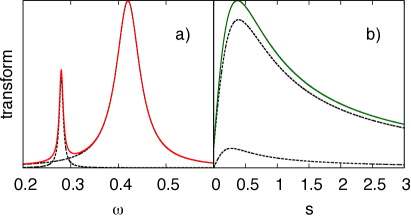
Figure 1: Fourier transform (left panel) and Laplace transform (right panel) of a memory kernel consisting of a superposition of two exponentially damped cosine functions. Their individual Laplace/Fourier counterparts are plotted in black dotted lines.

Another benefit of working in frequency domain is the possibility to limit the description to the region of the spectral density that is resonant with the system frequency only. This is illustrated in Fig. 2 by comparing the linear absorption spectra of a harmonic oscillator in a bath described by a spectral density with and without off-resonant contributions. The two spectra are almost identical and the influence of the off-resonant peaks in the spectral density on spectra is negligibly small, see insets therein, although the off-resonant peak intensity is about five times larger than the intensity in the resonant region. This is a manifestation of the well-known fact that the energy can be exchanged efficiently only when the bath is resonant with the system. Thus the consideration can be limited to a narrow frequency interval around the system frequency. In practice, this is a great simplification, since the spectral density might have an extremely elaborate pattern, if the bath consists of fairly complicated molecules, see, e.g. panel c) in Fig. 5. In time domain it would be impossible to filter out the corresponding signal. Importantly it would be equally complicated to extract the frequency window in Laplace domain due to the unsuitable shape of the Laplace-transformed damped oscillations, see panel b in Fig. 1.

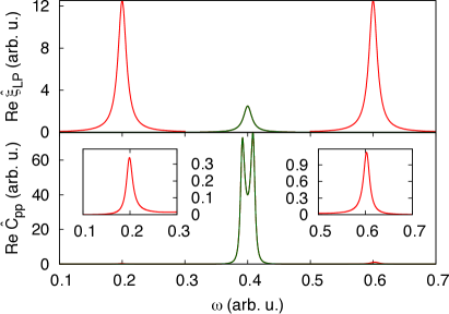
Figure 2: Two spectral densities, one having only the resonant contribution (green) and the other having additionally two off-resonant Lorentzian contributions (red) are depicted in the upper panel. The corresponding spectra of the harmonic oscillator with frequency $\bar{\omega}=0.4$ coupled to the spectral densities are shown in lower panel. Insets zoom on the spectral features stemming from the off-resonant contributions in the second spectral density.

To this end the problem of parametrizing GLE simulations seems to naturally pose itself in frequency domain, thereby operating with the spectral density rather than with the memory kernel. The transition from Laplace to frequency domain can be easily achieved by setting the Laplace variable imaginary, i.e. $s\equiv i\omega$ with a real frequency $\omega$. Equation (20) then becomes

$$i\omega\hat{C}_{pp}(\omega)-C_{pp}(t=0)=-\hat{K}_{\mathrm{LP}}(\omega)\hat{C}_{pp}(\omega)\enspace.$$ (21)

Solving Eq. (21) for the spectral density yields

$$\hat{K}_{\mathrm{LP}}(\omega)=\frac{1}{\hat{C}_{pp}(\omega)}-i\omega\enspace,$$ (22)

using that $C_{pp}(0)=1$ by normalization; note that the convolution theorem still applies to the half-sided Fourier transform.

Equation (22) is the starting point of the proposed Fourier-based GLE parametrization scheme, later referred to as the Fourier method, that is presented in detail in the next section.

III.5 Implementation of a Fourier Method

In this section we elaborate on setting up a GLE simulation according to Eq. (II.1) using the previously derived result in Eq. (22) as a starting point. Two quantities need to be calculated: the effective harmonic frequency, $\bar{\omega}$, defined in Eq. (4) and a spectral density $\hat{\xi}_{\mathrm{LP}}(\omega)$. Since the two memory kernels $\xi_{\mathrm{LP}}(t)$ and $K_{\mathrm{LP}}(t)$ differ only by the constant $\bar{\omega}^{2}$, the corresponding half-sided Fourier transforms are connected via

$$\hat{K}_{\mathrm{LP}}(\omega)=\hat{\xi}_{\mathrm{LP}}(\omega)+\pi\bar{\omega}^{2}\delta(\omega)-i\frac{\bar{\omega}^{2}}{\omega}\enspace.$$ (23)

One notices that the real parts of $\hat{\xi}_{\mathrm{LP}}(\omega)$ and $\hat{K}_{\mathrm{LP}}(\omega)$ coincide for $\omega>0$. Since the memory kernel $\xi_{\mathrm{LP}}(t)$ is a real function, the knowledge of the real part of $\hat{\xi}_{\mathrm{LP}}(\omega)$ and, thus, of $\hat{K}_{\mathrm{LP}}(\omega)$ is sufficient, because the imaginary part is provided by the Kramer-Kronig relations. Finally, fitting the hyperbola in the imaginary part of $\hat{K}_{\mathrm{LP}}(\omega)$ to the fit function $h(\omega)=-d/\omega$ provides an easy way to determine the effective harmonic frequency as $\bar{\omega}=\sqrt{d}$.

In order to use the obtained spectral density in GLE simulations, its corresponding memory kernel $\xi_{\mathrm{LP}}(t)$ must be given as a superposition of damped cosine functions, $f(t)=2a^{2}e^{-bt}\cos(ct),\ \forall a,b,c\in\mathbf{R},b>0$. The real part of its Fourier transform reads as a superposition of

$$\Re\hat{f}(\omega)=a^{2}b\cdot\left[\frac{1}{b^{2}+(c-\omega)^{2}}+\frac{1}{b^{2}+(c+\omega)^{2}}\right]\enspace,$$ (24)

which can in turn be used to fit the spectral density, $\hat{\xi}_{\mathrm{LP}}(\omega)$. For fitting the hyperbola in the imaginary part, $\Im\hat{K}_{\mathrm{LP}}(\omega)$, it is recommendable to subtract from it the imaginary parts of the fit functions given by

$$\Im\hat{f}(\omega)=a^{2}\cdot\left[\frac{c+\omega}{b^{2}+(c+\omega)^{2}}+\frac{c-\omega}{b^{2}+(c-\omega)^{2}}\right]\enspace.$$ (25)

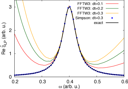
Figure 3: Real part of spectral densities obtained according to Eq. (22) for the test system, see text. The exact spectral density is shown in black. Numerical results obtained using the FFTW3 library for three time steps $0.1,0.2,0.3$ are shown in red, green and yellow, respectively. The result employing the Fourier transform based on the Simpson rule for a time step of $0.3$ is shown as blue dots.

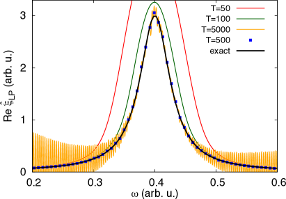
Figure 4: Real part of spectral densities obtained for the test system, see text, upon smoothing the MAF. The exact spectral density is shown in black. Results for different window widths $T=50,100,500,5000$ are shown as red, green, blue dots and yellow curves, respectively.

The performance of the method is illustrated on a simple test system: a harmonic oscillator ($\bar{\omega}=0.4$) in a bath described by a spectral density comprised of a single function as given in Eq. (24) with $a=0.03$, $b=0.03$ and $c=0.4$. In order to test the procedure, the aforementioned spectral density was used in GLE simulations to produce the MAF, that in turn was used to parametrize the spectral density as it was described above. The resulting spectral density was compared against the input one.

It turns out that the successful use of the procedure presented above rests upon two important numerical issues. First, the Fourier transform $\hat{C}_{pp}(\omega)$ needs to be calculated very accurately. In particular, performing the Fourier transform by means of the standard FFTW3 library Frigo and Johnson (2005) (based on a single-sided sum rule), led to diverging spectral densities even for moderate timestep sizes ($0.1-0.3$), that are typical for molecular systems with hydrogen atoms, if reasonable units (fs) are employed, see Fig. 3. Here, a more accurate quadrature, such as the 3/8 Simpson integration scheme, yielded excellent results already for a time step of $0.3$.

The second numerical issue concerns the usually insufficiently converged tail of the MAF, that causes noisy results upon the Fourier transform. In order to reduce the noise level we suggest Gaussian filtering, that is to multiply the MAF by a Gaussian window function

$$G(t)=\exp\left[-\frac{t^{2}}{2T^{2}}\right]\enspace.$$ (26)

In frequency domain this corresponds to a convolution with a Gaussian function of the width $\Delta\omega=1/T$ thereby suppressing the noise. The parameter $T$ should be chosen as a compromise between noise reduction and smoothing errors, see Fig. 4. As a rule of thumb, $T$ can be set equal to the correlation time in the system, which has been $T=500$ for our test system.

The developed parametrization method can be summarized by the following steps

• Calculate the MAF from explicit MD simulations with sufficient convergence (system dependent)

• Perform a reasonable Gaussian filtering to reduce the noise level upon the Fourier transform, taking the correlation time as a starting guess for the window width

• Transform MAF into frequency domain using a sufficiently accurate integrator, e.g. Simpson 3/8 rule

• Calculate the spectral density $\hat{K}_{\mathrm{LP}}(\omega)$ using Eq. (22)

• Estimate $\bar{\omega}$ and fit the real part of $\hat{K}_{\mathrm{LP}}(\omega)$ in its vicinity to superpositions of functions given in Eq. (24)

• Subtract the imaginary counterparts, Eq. (25) of the fit functions from $\Im\hat{K}_{\mathrm{LP}}(\omega)$

• Obtain the effective harmonic frequency $\bar{\omega}$ via a hyperbolic fit from the imaginary part of $\hat{K}_{\mathrm{LP}}(\omega)$

As a word of caution it should be stressed that the presented scheme does not give a correct estimate of a spectral density at low frequencies due to the divergence of $\hat{K}_{\mathrm{LP}}(\omega)$ at $\omega=0$ caused by the $\delta$-function, see Eq. (23). This leaves description of pure dephasing times outside reach.

IV Models and computational Details

We have investigated two hydrogen-bonded systems – HOD in H₂O, and the ionic liquid $[\mathrm{C}_{2}\mbox{mim}][\mbox{NTf}_{2}]$ at room temperature, as well as an A₂ in A model system employed by Berne et al. Berne et al. (1990). These examples have been chosen as water is perhaps the most important solvent and HOD features a spectrum with three distinct peaks, which makes it highly suitable for methodological investigations. Cho (2008); Giese et al. (2006); Habershon and Manolopoulos (2009); Ivanov et al. (2010); Stenger et al. (2001) The ionic liquid represents a system, where, in addition to moderate H-bonding, there exists a strong Coulomb interaction between the ion pairs Roth et al. (2012). Finally, investigating the A₂ in A model system allows us to compare our results with that of Berne et al, see Ref. Berne et al. (1990) for the parameters.

The aqueous systems have been comprised of 466 molecules in a periodic box with the length of $2.4\,$nm interacting according to the force field adopted from Ref. Paesani and Voth (2010). The harmonic HOD simulations used in Sec. V.3 for comparison, have been performed with exactly the same setup as the anharmonic ones, with the OH stretching potential in the HOD molecule being harmonic with the frequency obtained from expanding the respective Morse potential up to the second order ($\mu\omega^{2}=5081\,$kJ$\cdot$mol^-1Å^-2). The ionic liquid simulations have been carried out in a periodic box with the length of $4.5\,$nm containing 216 ionic pairs and the force field described in Ref. Köddermann et al. (2007). All explicit molecular dynamics (MD) simulations have been performed with the GROMACS program package (Version 4.6.5) Hess et al. (2008). The spectra have been computed for the OH stretch in the HOD molecule and for the C$(2)-$H stretch of the imidazolium ring Köddermann et al. (2007) in the ionic liquid. In the latter case the potential for the C-H stretching motion has been re-parametrized to a Morse potential using DFT-B3LYP calculations Zentel (2012). Note that in the spirit of the system-bath treatment the O-H bondlengths have been taken as the respective system coordinates, $x$, whereas all other degrees of freedom constituted the bath. We employed the “standard protocol” for calculating IR spectra, that is, a set of NVE trajectories, each $6\,$ps long (time step $0.1\,$fs), has been started from uncorrelated initial conditions sampled from an NVT ensemble. The dipole autocorrelation functions for the system coordinate have been Fourier-transformed to yield the spectra Ivanov et al. (2013). In order to achieve convergence, 1000 trajectories for the considered stretching motion have been employed.

For GLE simulations we adopted the method of Colored Noise thermostats Ceriotti et al. (2009b, 2010); Morrone et al. (2011), fitting the spectral density to a superposition of 8-12 functions as given in Eq. (24). In the GLE simulations all the numerical parameters for the time step, length, number of trajectories, etc. have been the same as in the explicit MD simulations. Bonds in the rigid bond approach have been fixed using the Settle algorithm as implemented in GROMACS.

V Numerical tests

In this section we first demonstrate that the proposed Fourier method provides accurate spectral densities that can describe realistic solute dynamics. Then the performance of the time domain techniques is discussed, using the spectral densities obtained via the Fourier method as a reference. Finally, an exceptional case for which the rigid bond approach works, the A₂ in A model system, is discussed in detail.

V.1 The Fourier method

In order to test the Fourier method, first the explicit MD simulations are performed and vibrational spectra and MAFs are calculated. Then the spectral densities are parametrized from these MAFs according to the Fourier method. These spectral densities are used as input for implicit GLE simulations, which in turn yield vibrational spectra that are compared against their explicit MD counterparts. The coincidence of the GLE and MD spectra manifests the success of the Fourier method.

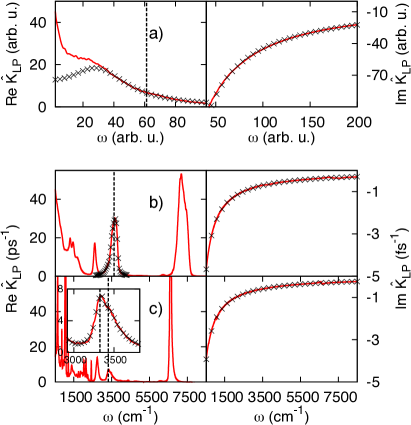
Figure 5: Real (left panels) and imaginary (right panels) parts of spectral densities (red curves) obtained according to the Fourier method are shown for a) A₂ in A, b) HOD in bulk water, and c) the ionic liquid. Vertical dashed lines denote the effective harmonic frequency $\bar{\omega}$. The fits to Lorentzian functions, Eq. (24), performed in the resonant region and the hyperbolic fits to the imaginary parts are depicted with black crosses. The inset in panel c) zooms into the resonant region. Note the different scales for imaginary and real parts.

In Fig. 5 the spectral densities, $\hat{K}_{\mathrm{LP}}(\omega)$, calculated according to Eq. (22), are shown for the three systems studied. The real parts of $\hat{K}_{\mathrm{LP}}(\omega)$ are depicted in the left panels therein. For the A₂ in A model system, panel a), the spectral density nicely reproduces that obtained by Berne et al. Berne et al. (1990) The spectral densities for the real systems considered, panels b) and c), possess peaked contributions at various frequencies stemming from the coupling to a plethora of vibrational modes in the bath. The spectral density is most structured in the ionic liquid case, panel c), due to the complexity of the molecules involved.

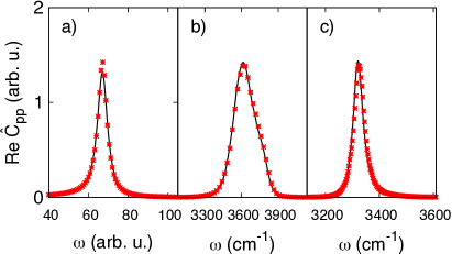
Figure 6: Explicit MD (black curve) and GLE spectra (red stars) shown for a) A₂ in A, b) HOD in bulk water and c) the ionic liquid.

However, as it was explained above, the only important region is in the vicinity of the system frequency $\bar{\omega}$, denoted by a dashed vertical line therein. The fits to the real part of spectral density in the important region, black crosses in Fig. 5, illustrate the excellent fit quality. Finally, one sees that the hyperbola in the imaginary part (right panels therein), Eq. (23), is clearly pronounced and can be thus very well fitted.

Having established the sufficient fit quality for the spectral densities, the GLE simulations are performed and the resulting vibrational spectra of the three investigated systems (red stars) are compared with that obtained from explicit MD simulations (black curves) in Fig. 6. It becomes apparent that the GLE simulations excellently reproduce the explicit MD spectra for all systems studied thereby confirming the success of the Fourier method as a parametrization scheme.

V.2 Comparison to Time Domain Techniques

Having obtained the numerical evidence that the spectral densities calculated from the Fourier method (red lines in Fig. 7) are reliable, we compare the results obtained via the rigid bond (blue) and Berne and Harp methods (green) against them.

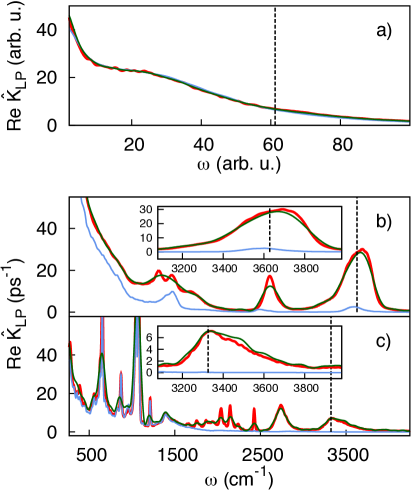
Figure 7: Real parts of the spectral densities obtained via the Fourier (red), rigid bond (blue) and Berne and Harp (green) methods are shown for a) A₂ in A b) HOD in bulk water and c) the ionic liquid. Dashed vertical lines mark $\bar{\omega}$ position. Insets zoom on the resonant regions.

One sees that the real parts of the spectral densities due to the Berne and Harp approach reproduce the reference results reasonably well. However, we encountered several numerical issues when using the method for the realistic systems studied. First, the polynomial interpolation turned out to be very sensitive to the degree $2n$ of the polynomial. In particular, using $n=1$ was insufficient, $n>2$ led to noticeable spikes causing divergences in the kernel and only $n=2$ yielded satisfactory results. Importantly, small inaccuracies in the polynomial interpolation turn out to accumulate strongly due to repeated integration according to Eq. (III.2). Second, even for $n=2$ the kernel diverged at long times and one had to cut it manually at the plateau, which could not be determined uniquely (data not shown). These deficiencies together with the general problems of time domain methods discussed in Sec. III.4 make the use of Berne and Harp method not convenient.

Considering the results of the rigid bond approach (blue lines in Fig. 7), one sees that it is successful only for the A₂ in A system, panel a) therein. The curves corresponding to realistic systems deviate from the reference results significantly. The general trend is that the larger is the frequency, the more the real part of the spectral density is downscaled. For HOD in water, panel b), noticeable deviations start from $\approx 1000\,$cm^-1, implying wrong description in the region where the bending and OH stretching modes reside. Remarkably, in the case of the ionic liquid, panel c), the frequency region below $1500\,$cm^-1 is well reproduced by the rigid system approach. In contrast, contributions to the important resonant region are completely absent in both cases, see insets in Fig. 7 for zoom on. Since the spectral densities obtained from the Fourier method are proven to be trustworthy, we thus conclude that the rigid system approach breaks down for the realistic cases considered here. According to the Laplace domain based analysis by Berne at al. Berne et al. (1990), see also Sec. III.3, this breakdown is no surprise since the rigid approach is valid only if the system frequency is high compared to that of bath modes. However, as it was discussed in Sec. III.4, it is more natural to consider the memory kernel in frequency domain. Here, the formula equivalent to Eq. (19) reads

$$\hat{\xi}_{\mathrm{RS}}(\omega)=\frac{\hat{\xi}_{\mathrm{LP}}(\omega)}{1+i\omega/(\bar{\omega}^{2}-\omega^{2})\hat{\xi}_{\mathrm{LP}}(\omega)}\enspace.$$ (27)

From this equation it becomes clear that a problem emerges for $\omega\rightarrow\bar{\omega}$, since the denominator diverges under the assumption that $\hat{\xi}_{\mathrm{LP}}(\omega)$ is finite in the vicinity of $\bar{\omega}$; note this assumption is not fulfilled the irrelevant case of isolated unperturbed systems. This divergence thus leads to vanishing $\hat{\xi}_{\mathrm{RS}}(\omega)$ in the mostly important resonant region. Since $\hat{\xi}_{\mathrm{RB}}(\omega)\approx\hat{\xi}_{\mathrm{RS}}(\omega)$ for sufficiently high frequency $\bar{\omega}$, see Sec. III.3, one can conclude that $\hat{\xi}_{\mathrm{RB}}(\omega)$ would vanish in the resonant region as well. Note that if the latter limit is not yet reached, then one observes a contribution at resonance, which corresponds to the error $\hat{\xi}_{\mathrm{RS}}(\bar{\omega})-\hat{\xi}_{\mathrm{RB}}(\bar{\omega})$. This explains our numerical results for the realistic systems studied, namely the absence of the signal for the ionic liquid and the small but finite contribution to the resonant region observed for the HOD in water case, see insets in panels b) and c). Interestingly, this line of reasoning suggests that having the frequency high can only make the situation worse, as then the error would become smaller and the spectral density even more underestimated. In fact, considering HOD in D₂O, where a frequency separation between the OH stretch and the bath modes was provided, fully confirmed this conjecture, did not improve the result (data not shown). Still, the low frequency region, $\omega\ll\bar{\omega}$, comes out correctly as it follows from this discussion and has been demonstrated numerically above.

Strictly speaking, the obtained spectral density is generally valid only for the particular (high frequency) mode studied, thus making this low frequency region irrelevant and the whole rigid bond approach inappropriate. An important consequence of the generally dramatic underestimation of the spectral density in the resonant region is the correspondingly overestimated energy relaxation time given in the framework of the Landau-Teller theory Tuckerman and Berne (1993) simply as $T_{1}=1/\hat{\xi}_{\mathrm{LP}}(\bar{\omega})$.

One might ask at this point, why the rigid bond method had success for the A₂ in A system, which we elaborate on in the next section.

V.3 Unexpected success of rigid bond method for A₂ in A

Let us consider what would happen if the system studied was indeed of the CL form. Then $\xi_{\mathrm{RB}}(t)=\xi_{\mathrm{CL}}(t)$ without any approximations. If further the model system potential, $V^{\prime}_{\mathrm{S}}(x)$, was harmonic then $\xi_{\mathrm{CL}}(t)$ and $\xi_{\mathrm{LP}}(t)$ would coincide up to a trivial offset. Since $\xi_{\mathrm{RB}}(t)=\xi_{\mathrm{LP}}(t)$ again up to a constant offset, $\xi_{\mathrm{RS}}(t)$ needs not to be considered. It suggests that the success of the rigid bond method for A₂ in A is based on the possibility that this system is indeed of the CL form.

In fact, Berne et al. Berne et al. (1990) have tested this conjecture by considering the temperature dependence of the static friction, $\hat{\xi}_{\mathrm{CL}}(\omega=0)$ and the frequency renormalisation term, $\xi_{\mathrm{CL}}(t=0)$. They concluded that the temperature dependence observed excludes the possibility of such a direct correspondence. However, the temperature was probed starting just above the melting point, which might have led to a significant change of the properties. Additionally, we have recently observed that the failure of such an indirect check does not necessarily lead to visible discrepancies in the observables, e.g. linear vibrational spectra. Ivanov et al. (2014) Particularly, testing the linearities of the coupling on both the system and bath sides for the very same realistic systems suggested that the latter is much more important than the former. Performing the same test for A₂ in A led to a strongly non-linear coupling on the system side and an almost ideally linear one on the bath side (data not shown). Therefore, the important linearity on the bath side suggests that the system can be represented by the CL model.

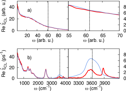
Figure 8: Real parts of the spectral densities for harmonic (red) and anharmonic (blue) system potentials are shown in the left panels for a) A₂ in A b) HOD in bulk water. Right panels zoom on the respective resonant regions.

Another possible check is provided by the independence of the spectral density in the CL model from the system potential, see Eq. (8). This can be tested by computing the memory kernel, $\xi_{\mathrm{CL}}(t)$, for both harmonic and anharmonic system potentials. It turned out that the spectral densities due to (an)harmonic system potentials coincide for A₂ in A, see panel a) in Fig. 8. A reference calculation performed for HOD in water revealed a striking discrepancy in the resonant region, panel b) therein.

These tests considered together indicate that A₂ in A can indeed be represented by the CL model. This also suggests that testing the dependence of the spectral density on the system potential is plausible.

VI Conclusions and Outlook

In this paper we considered the problem of parametrizing spectral densities within the linear GLE framework. We have shown that from the general perspective the problem naturally poses itself in the frequency domain, and both time and Laplace domains are not intrinsic to the problem. We have developed a Fourier-based method and compared its performance to the existing time-domain techniques, that is Berne and Harp Berne and Harp (1970) and the widely used rigid bond approach. It turned out that our method is extremely robust and provides trustworthy results for all systems studied. In contrast, Berne and Harp approach suffers from numerical problems apart from having general disadvantages of the time domain formulations. Surprisingly the rigid bond method, which is claimed to be accurate in the high frequency limit, turns out to be not appropriate in general, unless the system studied is of the Caldeira-Leggett form. Importantly, we have shown that the spectral densities due to the rigid bond method are strongly underestimated in the resonant region, which makes the common Landau-Teller estimation for the relaxation times questionable. A parametrizing scheme beyond the linear GLE regime, that is based on Eq. (14), has also been developed and will be published elsewhere.

The authors gratefully acknowledge financial support by the Deutsche Forschungsgemeinschaft (Sfb 652).

References

- May and Kühn (2011) V. May and O. Kühn, Charge and Energy Transfer Dynamics in Molecular Systems (Wiley-VCH, 2011).
- Lemons (1997) D. S. Lemons, Am. J. Phys. 65, 1079 (1997).
- Ornstein and Uhlenbeck (1930) L. S. Ornstein and G. E. Uhlenbeck, Phys. Rev. 36, 823 (1930).
- Zwanzig (2001) R. Zwanzig, Nonequilibrium Statistical Mechanics (Oxford University Press, 2001).
- Mori (1965) H. Mori, Prog. Theor. Phys. 33, 423 (1965).
- Zwanzig (1973) R. Zwanzig, J. Stat. Phys. 9, 215 (1973).
- Kawasaki (1973) K. Kawasaki, J. Phys. A Math. Nucl. Gen. 6, 1289 (1973).
- Whitnell et al. (1990) R. M. Whitnell, K. R. Wilson, and J. T. Hynes, J. Phys. Chem. 94, 8625 (1990).
- Benjamin and Whitnell (1993) I. Benjamin and R. M. Whitnell, Chem. Phys. Lett. 204, 45 (1993).
- Tuckerman and Berne (1993) M. Tuckerman and B. J. Berne, J. Chem. Phys. 98, 7301 (1993).
- Gnanakaran and Hochstrasser (1996) S. Gnanakaran and R. M. Hochstrasser, J. Chem. Phys. 105, 3486 (1996).
- Grote and Hynes (1980) R. F. Grote and J. T. Hynes, J. Chem. Phys. 73, 2715 (1980).
- Ceriotti et al. (2009a) M. Ceriotti, G. Bussi, and M. Parrinello, Phys. Rev. Lett. 103, 030603 (2009a).
- Ceriotti et al. (2009b) M. Ceriotti, G. Bussi, and M. Parrinello, Phys. Rev. Lett. 102, 020601 (2009b).
- Ceriotti et al. (2010) M. Ceriotti, G. Bussi, and M. Parrinello, J. Chem. Theory Comput. 6, 1170 (2010).
- Abe et al. (1996) Y. Abe, S. Ayik, P.-G. Reinhard, and E. Suraud, Phys. Rep. 275, 49 (1996).
- Tanimura (2006) Y. Tanimura, J. Phys. Soc. Japan 75, 1 (2006).
- Caldeira and Leggett (1981) A. Caldeira and A. Leggett, Phys. Rev. Lett. 46, 211 (1981).
- Caldeira and Leggett (1983a) A. O. Caldeira and A. J. Leggett, Ann. Phys. (N. Y). 149, 374 (1983a).
- Mukamel (1995) S. Mukamel, Principles of Nonlinear Optical Spectroscopy (Oxford University Press, Oxford, 1995).
- Palese and Mukamel (1996) S. Palese and S. Mukamel, J. Phys. Chem. 3654, 10380 (1996).
- Okumura and Tanimura (1997) K. Okumura and Y. Tanimura, J. Chem. Phys. 107, 2267 (1997).
- Woutersen and Bakker (1999) S. Woutersen and H. J. Bakker, Phys. Rev. Lett. 83, 2077 (1999).
- Toutounji and Small (2002) M. M. Toutounji and G. J. Small, J. Chem. Phys. 117, 3848 (2002).
- Tanimura and Ishizaki (2009) Y. Tanimura and A. Ishizaki, Acc. Chem. Res. 42, 1270 (2009).
- Joutsuka and Ando (2011) T. Joutsuka and K. Ando, J. Chem. Phys. 134, 204511 (2011).
- Kawai and Komatsuzaki (2011) S. Kawai and T. Komatsuzaki, J. Chem. Phys. 134, 114523 (2011).
- Cortes et al. (1985) E. Cortes, B. J. West, and K. Lindenberg, J. Chem. Phys. 82, 2708 (1985).
- Ford and Kac (1987) G. W. Ford and M. Kac, J. Stat. Phys. 46, 803 (1987).
- Ford et al. (1988) G. W. Ford, J. T. Lewis, and R. F. Oconnell, Phys. Rev. A 37, 4419 (1988).
- McDowell (2000) H. K. McDowell, J. Chem. Phys. 112, 6971 (2000).
- Banerjee et al. (2004) D. Banerjee, B. C. Bag, S. K. Banik, and D. S. Ray, J. Chem. Phys. 120, 8960 (2004).
- Feynman and Vernon (1963) R. Feynman and F. Vernon, Ann. Phys. (N. Y). 24, 118 (1963).
- Caldeira and Leggett (1983b) A. Caldeira and A. Leggett, Phys. A Stat. Mech. its Appl. 121, 587 (1983b).
- Dijkstra and Tanimura (2010) A. G. Dijkstra and Y. Tanimura, Phys. Rev. Lett. 104, 250401 (2010), arXiv:1004.1450 .
- Suess et al. (2014) D. Suess, A. Eisfeld, and W. T. Strunz, Phys. Rev. Lett. 113, 150403 (2014).
- Giese et al. (2006) K. Giese, M. Petković, H. Naundorf, and O. Kühn, Phys. Rep. 430, 211 (2006).
- Egorov et al. (1999) S. A. Egorov, E. Rabani, and B. J. Berne, J. Chem. Phys. 110, 5238 (1999).
- Baczewski and Bond (2013) A. D. Baczewski and S. D. Bond, J. Chem. Phys. 139, 044107 (2013).
- Stella et al. (2014) L. Stella, C. D. Lorenz, and L. Kantorovich, Phys. Rev. B 89, 134303 (2014).
- Ivanov et al. (2014) S. D. Ivanov, F. Gottwald, and O. Kühn, ArXiv e-prints (2014), arXiv:1412.1688 [physics.chem-ph], arXiv:0707.3168 [hep-th] .
- Kühn and Naundorf (2003) O. Kühn and H. Naundorf, Phys. Chem. Chem. Phys. 5, 79 (2003).
- Berne et al. (1990) B. J. Berne, M. E. Tuckerman, J. E. Straub, and A. L. R. Bug, J. Chem. Phys. 93, 5084 (1990).
- Berne and Harp (1970) B. J. Berne and G. D. Harp, Adv. Chem. Phys 17, 63 (1970).
- Berkowitz et al. (1981) M. Berkowitz, J. D. Morgan, D. J. Kouri, and J. A. McCammon, J. Chem. Phys. 75, 2462 (1981).
- Lange and Grubmüller (2006) O. F. Lange and H. Grubmüller, J. Chem. Phys. 124, 214903 (2006).
- Shin et al. (2010) H. K. Shin, C. Kim, P. Talkner, and E. K. Lee, Chem. Phys. 375, 316 (2010).
- Straub et al. (1987) J. E. Straub, M. Borkovec, and B. J. Berne, J. Phys. Chem. 91, 4995 (1987).
- Goodyear and Stratt (1996) G. Goodyear and R. M. Stratt, J. Chem. Phys. 105, 10050 (1996).
- Berkowitz et al. (1983) M. Berkowitz, J. D. Morgan, and J. A. McCammon, J. Chem. Phys. 78, 3256 (1983).
- Grabert et al. (1988) H. Grabert, P. Schramm, and G.-L. Ingold, Phys. Rep. 168, 115 (1988).
- Todd (1962) J. Todd, Survey of Numerical Analysis (McGraw-Hill, 1962).
- Day (1967) J. T. Day, Bit 7, 71 (1967).
- Morrone et al. (2011) J. A. Morrone, T. E. Markland, M. Ceriotti, and B. J. Berne, J. Chem. Phys. 134, 014103 (2011).
- Frigo and Johnson (2005) M. Frigo and S. G. Johnson, Proceedings of the IEEE 93, 216 (2005), special issue on “Program Generation, Optimization, and Platform Adaptation”.
- Cho (2008) M. Cho, Chem. Rev. 108, 1331 (2008).
- Habershon and Manolopoulos (2009) S. Habershon and D. E. Manolopoulos, J. Chem. Phys. 131, 244518 (2009).
- Ivanov et al. (2010) S. D. Ivanov, A. Witt, M. Shiga, and D. Marx, J. Chem. Phys. 132, 031101 (2010).
- Stenger et al. (2001) J. Stenger, D. Madsen, P. Hamm, E. T. J. Nibbering, and T. Elsaesser, Phys. Rev. Lett. 87, 027401 (2001).
- Roth et al. (2012) C. Roth, S. Chatzipapadopoulos, D. Kerlé, F. Friedriszik, M. Lütgens, S. Lochbrunner, O. Kühn, and R. Ludwig, New J. Phys. 14, 105026 (2012).
- Paesani and Voth (2010) F. Paesani and G. A. Voth, J. Chem. Phys. 132, 014105 (2010).
- Köddermann et al. (2007) T. Köddermann, D. Paschek, and R. Ludwig, ChemPhysChem 8, 2464 (2007).
- Hess et al. (2008) B. Hess, C. Kutzner, D. van der Spoel, and E. Lindahl, J. Chem. Theory Comput. 4, 435 (2008).
- Zentel (2012) T. Zentel, (Non-)linear Spectroscopy Based on Classical Trajectories, Master’s thesis, Rostock University, Rostock, Germany (2012), uRL: http://rosdok.uni-rostock.de/resolve/id/rosdok_thesis_0000000013.
- Ivanov et al. (2013) S. D. Ivanov, A. Witt, and D. Marx, Phys. Chem. Chem. Phys. 15, 10270 (2013).