Magnetic and Nonmagnetic Phases in Doped $AB_{2}$ $t$-$J$ Chains

Abstract

We discuss the rich phase diagram of doped $AB_{2}$ $t$-$J$ chains using data from DMRG and exact diagonalization techniques. The $J$ vs $\delta$ (hole doping) phase diagram exhibits regions of itinerant ferrimagnetism, Incommensurate, RVB, and Nagaoka States, Phase Separation, and Luttinger Liquid (LL) Physics. Several features are highlighted, such as the modulated ferrimagnetic structure, the occurrence of Nagaoka spin polarons in the underdoped regime and small values of $J=4t^{2}/U$, where $t$ is the first-neighbor hopping amplitude and $U$ is the on-site repulsive Coulomb interaction, incommensurate structures with nonzero magnetization, and the strong-coupling LL physics in the high-doped regime. We also verify that relevant findings are in agreement with the corresponding ones in the square and $n$-leg ladder lattices. In particular, we mention the instability of Nagaoka ferromagnetism against $J$ and $\delta$.

I Introduction

The $t$-$J$ version of the Hubbard Hamiltonian montorsi is a key model for the understanding of strongly correlated electron systems. The model is defined through only two competing parameters: the hopping integral $t$, which measures the electron delocalization through the lattice, and the exchange coupling $J=4t^{2}/U$, where $U>>t$ is the on-site Coulomb repulsion. In fact, several versions of the simplest Hubbard Hamiltonian, with a single orbital at each lattice and the on-site Coulomb repulsion, have been extensively used to model a variety of phenomena, such as: metal-insulator transition gebhard ; *Imada, quantum magnetism auerbach and High-$T_{c}$ superconductivity and_sce_ht . Moreover, exact solutions montorsi and rigorous results liebwu ; *kor2005; RevLieb ; *tasakihubrev; *revtian have played a central role in this endeavor.

We emphasize Lieb’s theorem PRLLIEB , a generalization of the one by Lieb and Mattis LiebMattis for Heisenberg systems, which asserts that the ground state (GS) total spin of a bipartite lattice at half filling and $U>0$ is given by $S_{GS}=|N_{A}-N_{B}|/2$, where $N_{A}$ ($N_{B}$) is the number of sites on sublattice $A$ ($B$); indeed, Lieb’s theorem has greatly enhanced the investigation of new aspects of quantum magnetism RevLieb ; *tasakihubrev; *revtian. In particular, we mention the occurrence of ferrimagnetic GS, in which case we select studies using Hubbard or $t$-$J$ models PRLMDCF95 ; PRBTIAN ; LiangWang ; SierraPRB1999 ; *sierraprb2005; MontenegroPRB2006 ; OliveiraPRB2009 ; lopes2011 ; *lopes2014; *[ForBose-Hubbardmodels; see][]NJP; *Aoki, including the Heisenberg strong-coupling limit PRLRAPOSO97 ; *PRBRAPOSO1999; *SW; CINV ; PhysA ; *YamamotoPRB2007, on chains with $AB_{2}$ or $ABC$ topological structures with $S_{GS}=1/2$ per unit cell PRLMDCF95 ; PRLRAPOSO97 ; *PRBRAPOSO1999; *SW; CINV ; PRBTIAN ; LiangWang ; SierraPRB1999 ; *sierraprb2005; MontenegroPRB2006 ; *OliveiraPRB2009, which implies ferromagnetic and antiferromagnetic long-range orders PRBTIAN . Further, the inclusion of competing interactions or geometrical and kinetic frustration IvCONDMAT2009 ; frustrIn ; *Nakano; *furuya; lyra1 ; *lyra2; *Rojas2012, enlarge the classes of models, thereby allowing ground-states not obeying Lieb or Lieb and Mattis theorems. These studies have proved effective in describing magnetic and other physical properties of a variety of organic, organometallic, and inorganic quasi-one-dimensional compounds COUTINHO-FILHO2008 ; IvCONDMAT2009 .

Of particular physical interest are doped systems, although in this case rigorous results are much rare RevLieb ; *tasakihubrev; *revtian. One exception is Nagaoka’s theorem nagaoka , which asserts that for $J=0$ ($U\rightarrow\infty$) the $t$-$J$ model with one hole added to the undoped system (half-filled band) is a fully polarized ferromagnet, favored by the hole kinematics, if the lattice satisfies the so-called connectivity condition tasaki . A long-standing problem about this issue is the stability of the ferromagnetic state for finite hole densities and finite values of $J$. Numerical results have indicated PhysRevLett.108.126406 ; 2D_F that two-dimensional lattices display a fully polarized GS for $J=0$ and $\delta\lesssim 0.2$, where $\delta=N_{h}/N$, with $N_{h}$ ($N$) the total number of holes (sites); while, analytical studies Altshuler ; PhysRevB.85.245113 have suggested that this state is stable up to $J_{t}\sim\delta^{2}$.

Further, an ubiquitous phenomenon in doped strongly correlated materials is the occurrence of inhomogeneous states, particularly spatial phase separation in nano- and mesoscopic scales dagotto and incommensurate states dagotto ; Inc . In underdoped High-$T_{c}$ materials, dynamical and statical stripes in copper oxide planes has been the focus of intensive research Revtranquada . Concerning two-dimensional $t$-$J$ or Hubbard models, phase separation into hole-rich and no-hole regions was discussed in the large$-$ and small$-J$ limits emery . However the precise charge distribution in the ground state remains controversial. The use of distinct and refined numerical methods have pointed to striped PhysRevB.84.041108 or uniform phases PhysRevB.85.081110 ; recently, it was claimed that the origin of this issue relies on the strong competition between these phases corboz . For the linear $t$-$J$ Hubbard chain the physics is more clear ogatta , and phase separation takes place for $J=2.5-3.0$, depending on the doping value, but it is absent in the small$-J$ regime.

In this work, we use Density Matrix Renormalization Group (DMRG) DMRG technique and Lanczos exact diagonalization (ED) to obtain the ground state phase diagram and the low-energy excitations properties of the doped $t$-$J$ model on $AB_{2}$ chains PRLMDCF95 for $J=0.0-0.4$. We verify the occurrence of an itinerant modulated ferrimagnetic (FERRI) phase in the underdoped regime, regions of incommensurate (IC) states and Nagaoka ferromagnetism (F), and two regions of phase separation (PS), in which IC and F states coexist with the resonating valence bond state (RVB), respectively. In addition, we find that the RVB state is the stable phase at $\delta=1/3$, and identify a crossover region that ends at the onset of a Luttinger liquid (LL) phase at $\delta=2/3$, above which the LL physics luttinger sets in.

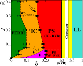
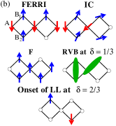
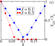
Figure 1: (Color online). (a) GS phase diagram for the $AB_{2}$ $t$-$J$ model (error bars account for the discrete values assumed by $\delta$ in a finite-size system). The phases are illustrated in (b): modulated ferrimagnetism (FERRI), incommensurate (IC), Nagaoka ferromagnetism (F), short-range resonating valence bond (RVB) states, phase separation (PS), and Luttinger liquid (LL). The estimated transition lines $\delta_{FERRI,J}$, $\delta_{PS,J}$, and $J_{F,\delta}$ are also pointed out. (c) Ground state total spin, $S_{GS}$, normalized by its value in the undoped regime: $S_{L}\equiv(N_{c}/2)-0.5$, as function of $\delta$ for the indicated values of $J$ and $N=3N_{c}+1=100$.

II Phase Diagram

The $t$-$J$ model reads:

$$H_{t-J} =-t\sum_{<i,j>,\sigma}P_{G}(c^{\dagger}_{i\sigma}c_{j\sigma}+H.c.)P_{G}$$ (1)

$${}+J\sum_{<i,j>}(\mathbf{S}_{i}\cdot\mathbf{S}_{j}-\frac{1}{4}n_{i}n_{j}),$$

where $c_{i\sigma}$ annihilates electrons of spin $\sigma$ at site $i$, $n_{i}$ is the number operator at site $i$ and $P_{G}=\prod_{i}(1-n_{i\uparrow}n_{i\downarrow})$ is the Gutzwiller projector operator that excludes states with doubly occupied sites. In our simulations, we set $t=1$ and have considered chains with $N_{c}$ $(N)$ unit cells (sites). In ED calculations closed boundary conditions are used with $N_{c}=8$ $(N=3N_{c})$, while in the DMRG simulations open boundary conditions are used and the system sizes ranged from $N_{c}=33$ $(N=3N_{c}+1=100)$ to $N_{c}=121$ $(N=364)$. We retain from 243 to 364 states in the DMRG calculations, and the typical discarded weight is $1\times 10^{-7}$.

The ground state (GS) phase diagram, shown in Fig. 1 (a), displays the regions of the above-mentioned phases, illustrated in Fig. 1(b), including the estimated transition lines and the crossover region. A special feature of the $AB_{2}$ chain is its symmetry CINV ; SierraPRB1999 ; *sierraprb2005; MontenegroPRB2006 ; *OliveiraPRB2009 under the exchange of the labels of the $B$ sites in a given unit cell $l$ [identified in the FERRI state, Fig. 1(b)]. This symmetry implies in a conserved parity $p_{l}=\pm 1$ in each cell of the lattice. The phase diagram of a chain with $N_{c}$ unit cells is calculated by obtaining the lowest energy for all subspaces with $x$ contiguous cells of parity $-1$ and the others $N_{c}-x$ cells with parity $+1$, with $x=0\ldots N_{c}$, for fixed $\delta$ and $J$. In the phase diagram shown in Fig. 1(a), $p\equiv\sum_{i=1}^{N_{c}}p_{l}=+1$ for $\delta\geq 1/3$, $p\neq\pm 1$ in the PS region, and $p=-1$ for $\delta<\delta_{PS,J}$. The magnetic configuration of a phase is identified by the total spin $S_{GS}$, local magnetization, magnetic structure factor, and spin correlation functions. In what follows, we shall characterize the phases shown in Fig. 1(a).

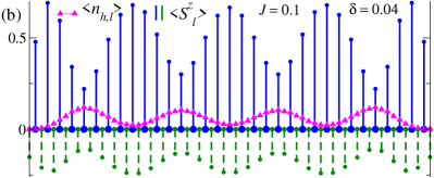
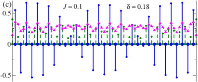
Figure 2: (Color online). (a) Effective linear chain (spacing $a\equiv 1$) associated with $N=3N_{c}+1=100$ sites for $J=0.1$ used to illustrate the hole, $\langle n_{h,l}\rangle$, and spin, $\langle S^{z}_{l}\rangle$, profiles: (b) $\delta=4/100$ (FERRI phase) and (c) $\delta=18/100$ (IC phase).

III Ferrimagnetism and transition to IC states

At $\delta=0$ and $J\neq 0$, the insulating Lieb ferrimagnetic state with total spin quantum number $S_{GS}=S_{L}\equiv N_{c}/2-0.5\equiv S_{L}$ is found for a chain with open boundary conditions, $N=3N_{c}+1=100$, with an $A$ site on each side. In order to evaluate the stability of this state against doping, we calculate $S_{GS}$ as a function of $\delta$ from the energy degeneracy in $S^{z}$. As shown in Fig. 1(c), as hole doping increases from $\delta=0$ to a critical value $\delta=\delta_{FERRI,J}$, the value of $S_{GS}$ decreases linearly from $S_{L}$ to 0 or a residual value, signaling a smooth transition to the IC phase. However, for low enough $J$, $S_{GS}$ of the IC phase increases linearly with $\delta$ up to $\delta=\delta_{PS,J}$, the line at which PS occurs [see Fig. 1(a)], or up to the boundary, $J_{F,\delta}$, of the Nagaoka F phase. This unexpected behavior claims for an explanation.

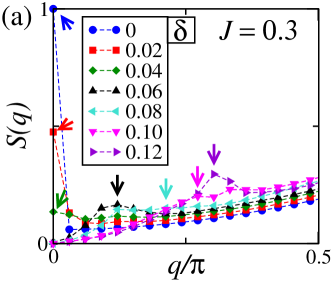
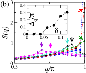
Figure 3: (Color online). Chain with $N=3N_{c}+1=100$ and $J=0.3$. (a) and (b): Magnetic structure factor $S(q)$ for the indicated values of $\delta$. Inset of (b): $\Delta_{q}\equiv q_{\text{max}}-\pi$, where $q_{\text{max}}$ is the value of $q$ at which the local maximum of $S(q)$, near $q=\pi$, is observed.

In order to understand the behavior of $S_{GS}$ for low $J$ we have calculated the profiles of the magnetization, $\langle S^{z}_{l}\rangle$, in the spin sector $S^{z}=S_{GS}$, and of the hole density, $\langle n_{h,l}\rangle$, for $J=0.1$ (see Fig. 2). To help in the data visualization, we use a linearized version of the lattice, as illustrated in Fig. 2(a). As shown in Fig. 2(b), for $\delta=0.04$ the holes distort the ferrimagnetic structure, which display a modulation with wavelength $\lambda\approx 17$, in anti-phase with that exhibited by the hole (charge) density wave. We have thus identified a modulated itinerant ferrimagnetic phase in this underdoped regime. On the other hand, as shown in Fig. 2(c), for $\delta=0.18$ the magnetization has local maxima in coincidence with those of the hole density profile. In this case, the IC phase is characterized by the presence of ferromagnetic Nagaoka spin polarons PhysRevB.85.245113 ; polaron due to hole density wave with $\lambda\approx 4$. Our results point to a value of $J$ ($\sim 0.2$) below which ferromagnetic “bubbles” appear as precursors of the F phase found for $J<J_{F,\delta}$ [see Fig. 1(a)].

For $J=0.3$, $S_{GS}=0$ in the IC phase, as shown in Fig. 1(c). In Figs. 4 (a) and (b) we present the magnetic structure factor

$$S(q)=\frac{1}{S_{L}(S_{L}+1)}\sum_{l,m}^{2N_{c}+1}e^{iq(l-m)}\langle\mathbf{S}_{l}\cdot\mathbf{S}_{m}\rangle,$$ (2)

where $l$, $m$ and $\mathbf{S}$ refer to the lattice representation shown in Fig. 2(a), for this value of $J$ and doping ranging from $\delta=0$ up to $\delta=0.12$. In a long-range ordered ferrimagnetic state, sharp maxima at $q=0$ (ferromagnetism) and $q=\pi$ (antiferromagnetism) are observed in the curve $S(q)$ for $\delta=0$. Adding two holes to the undoped state, sharp maxima at $q=0$ and $\pi$ are also observed, while broad maxima occur for $\delta=0.04$, indicating short-range ferrimagnetic order which evolves to the IC phase by increasing doping, before phase separation (IC-RVB) at the line $\delta=\delta_{PS,J}$ [see Fig. 1(a)]. In the inset of Fig. 4(b) we show the departure of the maximum of $S(q)$ from $q=\pi$.

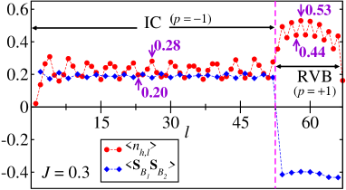
Figure 4: (Color online). Phase separation (IC-RVB) for a chain with $N=3N_{c}+1=100$ sites, $J=0.3$, and $N_{h}=18$ holes: spin correlation function between $B$ spins at the same cell, $\langle\mathbf{S}_{B_{1},l}\cdot\mathbf{S}_{B_{2},l}\rangle$, and hole density profile, $\langle n_{h,l}\rangle$.

IV Phase Separation, RVB states and Luttinger Liquid

In Fig. 1(a) the dashed line inside the PS region fix the boundary between two types of phase separation: in one case, the separation occurs between Nagaoka ferromagnetism and short-range RVB states (F-RVB); while in the other, it occurs between IC and short-range RVB states (IC-RVB). Indeed, for $0\leq J\lesssim 0.063$ and $\delta_{F-RVB}\leq\delta<1/3$, the GS phase separates with F and short range RVB states under coexistence, where $\delta_{F-RVB}$ denotes hole density values along the phase separation line F-RVB, thereby extending our previous result MontenegroPRB2006 ; OliveiraPRB2009 valid only for $J=0$. However, for $0.063\lesssim J\leq 0.4$ the system behaves differently. The new PS (IC-RVB) region is here illustrated for $J=0.3$, $N=3N_{c}+1=100$ sites, and $N_{h}=18$ holes: we thus find that there are 26 cells with odd parity ($p_{l}=-1$), associated with the IC phase, and the remaining 7 cells with even parity ($p_{l}=+1$), associated with the RVB phase. In this case, as shown in Fig. 4(c), the hole-poor IC phase presents a local spin correlation function $\langle\mathbf{S}_{B_{1},l}\cdot\mathbf{S}_{B_{2},l}\rangle\approx 0.2$, average hole density per site $\approx 0.16$, estimated from the sites indicated by arrows [one $A$ site and two $B$ sites in the context of the effective linear chain shown in Fig. 2(a)], and hole-density wave with $\lambda\approx 4$; while the hole-rich RVB phase presents $\langle\mathbf{S}_{B_{1},l}\cdot\mathbf{S}_{B_{2},l}\rangle\approx-0.4$ and average hole density per site $\approx 1/3$, estimated from a cell with $A$ and $B$ sites indicated by arrows. Therefore, apart from boundary effects, the above results thus indicate that the phase separation for a given $J$ value is defined by the coexistence of the two phases with the hole densities $\delta_{IC\text{-}PS}$ ($\approx 0.16$ for $J=0.3$) and $\delta_{PS\text{-}RVB}$ ($\approx 1/3$ for $J=0.3$) fixed at the IC-PS and PS-RVB boundaries, respectively, while the size of the phases are fixed by the chemical doping $\delta=N_{h}/N$ ($=0.18$ for $N=100$ and $N_{h}=18$). We also remark that the stable RVB phase observed at $\delta=1/3$ and $0\leq J\leq 0.4$, which has finite charge and spin gaps, is in agreement with predictions for $J=0.35$ SierraPRB1999 ; *sierraprb2005 and $J=0$ MontenegroPRB2006 ; OliveiraPRB2009 .

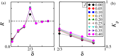
Figure 5: (Color online). Luttinger liquid behavior for a chain with $N=3N_{c}=24$ (ED results). (a) Ratio $R=u_{\rho}/\sqrt{D\chi/\pi}$ as a function of $\delta$ for the indicated values of $J$. (b) Exponent $K_{\rho}$ as a function of $\delta$.

For $0\leq J\leq 0.4$ and $1/3<\delta<2/3$, a crossover region with the presence of long-range RVB states after hole addition away from $\delta=1/3$ is observed [see Fig. 1(a)]. At the commensurate filling $\delta=2/3$, the system presents a charge gap, while the spin excitation is gapless, also extending our previous result for $J=0$ MontenegroPRB2006 ; OliveiraPRB2009 .

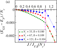
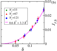
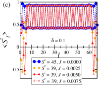
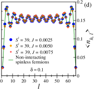
Figure 6: (Color online). (a) Shift $E_{GS}-E_{F}$ per unit cell, where $E_{F}$ is the energy of the fully polarized ferromagnetic state, as a function of $J/J_{F,\delta}$ for the indicated values of $N_{c}$ and $\delta$. (b) Instability line of the Nagaoka ferromagnetic phase. (c) Spin and (d) hole profiles, $\langle n_{h,l}\rangle$ and $\langle S^{z}_{l}\rangle$, respectively, for a chain with $N=3N_{c}+1=100$, $\delta=0.1$, and the indicated values of $S^{z}$ and $J$.

With the aim of investigating the LL behavior as a function of $J$ and $\delta\geq 2/3$, we have calculated, through ED techniques, the ratio $R=u_{\rho}/\sqrt{D\chi/\pi},$ where

$$\chi=\frac{N_{c}}{4}[E(N_{h}+2)+E(N_{h}-2)-2E_{GS}(N_{h})]$$ (3)

is the charge susceptibility, and $E(N_{h}\pm 2)$ is the total energy for $N_{h}\pm 2$ holes;

$$D=\frac{N_{c}}{4\pi}\left[\frac{\partial^{2}E(\Phi)}{\partial\Phi^{2}}\right]_{\Phi_{min}}$$ (4)

is the Drude weight, where $E(\Phi)$ is the lowest energy for a magnetic flux $\Phi$ through a closed chain, and $\Phi_{min}$ its value at $E_{GS}$;

$$u_{\rho}=\frac{{E(k_{GS}+\Delta k,S=0)-E_{GS}(k_{GS},S_{GS}=0)}}{\Delta k}$$ (5)

is the charge excitation velocity, where $\Delta k=2\pi/N_{c}$, and $E(k_{GS}+\Delta k,S=0)$ is the lowest energy with wavenumber $k=k_{GS}+\Delta k$ and total spin $S=S_{GS}=0$. If the low-energy physics of the system is that of a LL, we should find $R=1$ poilblanc ; moreover, the exponent governing the asymptotic behavior of the correlation functions, $K_{\rho}$, satisfies the relation $K_{\rho}=\pi u_{\rho}/2\chi$. As shown in Fig. 5(a), $R$ is indeed very close to 1 for $\delta>2/3$; in addition, as shown in Fig. 5(b), we find $0.7\gtrsim K_{\rho}\gtrsim 0.5$ for $\delta>2/3$. Remarkably, as shown in Figs. 5(a) and (b), the data for $R$ and $K_{\rho}$ exhibit data collapse as a function of $\delta$ for $0\leq J\leq 0.4$. In short, the results above clearly indicate that for $\delta>2/3$ and $0\leq J\leq 0.4$ the system behaves as a LL in the strong coupling regime.

V Stability of Nagaoka ferromagnetism

In this Section, we shall provide strong evidence that for $0\leq J\leq J_{F,\delta}$ and $0<\delta\leq\delta_{F-RVB}$, the kinetic energy of holes is lowered in a fully polarized ferromagnetic state, an extension of Nagaoka ferromagnetism nagaoka ; tasaki , with the GS energy equal to that of non-interacting spinless fermions: $E_{GS}=E_{F}$.

The estimate of $J_{F,\delta}$ is based on the data for the shift $(E_{GS}-E_{F})/N_{c}$ as a function of $J$, as illustrated in Fig. 6(a) for $\delta$ close or equal to 0.1. We stress that the shift decreases as $N_{c}$ increases for $0<(J/J_{F,\delta})<1$, and goes to zero in the thermodynamic limit. In addition, one should notice that, by examining the data above and below $J=J_{F,\delta}$, particularly for $N=3N_{c}+1=364$ sites, $\partial{E_{GS}}/\partial{J}$ appears to be discontinuous at $J=J_{F,\delta}$ in the thermodynamic limit, thus suggesting a first-order transition to the IC phase at $(J/J_{F,\delta})=1$. In Fig. 6(b) we show that our estimated transition line, $J_{F,\delta}$, [see also Fig. 1(a)] is almost not affected by finite size effects and implies $\delta_{F,J}\sim\sqrt{J}$ as $\delta\rightarrow 0$, as found from analytical results Altshuler ; PhysRevB.85.245113 for the $t$-$J$ model in a square lattice. In particular, for $J=0$ the instability of the Nagaoka state occurs at $\delta\approx 0.23$, which is very close to the values of hole doping estimated for $n$-leg ladder systems PhysRevLett.108.126406 and the square lattice PhysRevLett.108.126406 ; 2D_F .

The spin profile for a chain with $N=3N_{c}+1=100$, $J\gtrsim 0$ and $\delta=0.1$ is also in very good agreement with the Nagaoka state, as shown in Fig. 6(c), although boundary effects are visible for $J\gtrsim 0$; in fact, $S^{z}$ changes from 45 to 39 (on average, three spins at each boundary are not fully polarized), but one should notice that the change saturates as $J$ slightly increases above zero. This fact is corroborated by the hole density shown in Fig. 6(d), whose data for the referred states with $S^{z}=39$ at $\delta=0.1$ are very well described by the Nagaoka profile.

VI Discussion and Concluding Remarks

The presented phase diagram of doped $AB_{2}$ $t$-$J$ chains is remarkably rich. Indeed, several magnetic and nonmagnetic phases manifest themselves in a succession of surprising relevant features, some of which are similar to those observed in the square and $n$-leg ladder lattices: all in a simple doped chain. In particular, we emphasize the modulated ferrimagnetic structure, the occurrence of Nagaoka spin polarons in the underdoped regime and small values of $J$, incommensurate structures with nonzero magnetization, the strong-coupling LL physics in the high-doped regime, and the instability of Nagaoka ferromagnetism against $J$ and doping. Therefore, these chains are unique systems and of relevance for the physics of polymeric materials, whose properties might also represent challenging topics to be explored via analog simulations in ultracold fermionic optical lattices.

This work was supported by CNPq and FACEPE through the PRONEX program, and CAPES (Brazilian agencies).

References

- (1) The Hubbard Model – A Reprint Volume, edited by A. Montorsi (World Scientific, Singapore, 1992)
- (2) F. Gebhard, The Mott Metal-Insulator Transition (Springer, Berlin, 1997)
- (3) M. Imada, A. Fujimori, and Y. Tokura, Rev. Mod. Phys. 70, 1039 (1998)
- (4) A. Auerbach, Interacting Electrons and Quantum Magnetism (Springer, Berlin, 1998)
- (5) P. W. Anderson, Science 235, 1196 (1987); The Theory of Superconductivity in the High-Tc Cuprates (Princeton University Press, Princeton, 1997); P. A. Lee, N. Nagaosa, and X.-G. Wen, Rev. Mod. Phys. 78, 17 (2006)
- (6) E. H. Lieb and F. Y. Wu, Phys. Rev. Lett. 20, 1445 (1968)
- (7) F. H. L. Essler, H. Frahm, F. Gohmann, A. Klumper, and V. E. Korepin, The One-Dimensional Hubbard Model (Cambridge University Press, Cambridge, 2005)
- (8) E. H. Lieb, in The Hubbard model, its Physics and Mathematical Physics, Nato ASI, Series B: Physics, Vol. 343, edited by Baeriswyl, D. K. Campbell, J. M. P. Carmelo, F. Guinea, and E. Louis (Plenum, New York, 1995)
- (9) H. Tasaki, J. Phys.: Condens. Matt. 10, 4353 (1998)
- (10) G.-S. Tian, J. Stat. Phys. 116, 629 (2004)
- (11) E. H. Lieb, Phys. Rev. Lett. 62, 1201 (1989)
- (12) E. Lieb and D. Mattis, J. Math. Phys. 3, 749 (1962)
- (13) A. M. S. Macêdo, M. C. dos Santos, M. D. Coutinho-Filho, and C. A. Macêdo, Phys. Rev. Lett. 74, 1851 (1995)
- (14) G.-S. Tian and T.-H. Lin, Phys. Rev. B 53, 8196 (1996)
- (15) S.-D. Liang, Z. D. Wang, Q. Wang, and S.-Q. Shen, Phys. Rev. B 59, 3321 (1999)
- (16) G. Sierra, M. A. Martín-Delgado, S. R. White, D. J. Scalapino, and J. Dukelsky, Phys. Rev. B 59, 7973 (1999)
- (17) M. A. Martín-Delgado, J. Rodriguez-Laguna, and G. Sierra, ibid. 72, 104435 (2005)
- (18) R. R. Montenegro-Filho and M. D. Coutinho-Filho, Phys. Rev. B 74, 125117 (2006)
- (19) M. H. Oliveira, E. P. Raposo, and M. D. Coutinho-Filho, Phys. Rev. B 80, 205119 (2009)
- (20) A. A. Lopes and R. G. Dias, Phys. Rev. B 84, 085124 (2011)
- (21) A. A. Lopes, B. A. Z. António, and R. G. Dias, Phys. Rev. B 89, 235418 (2014)
- (22) J. J. García-Ripoll and J. K. Pachos, New Journal of Physics 9, 139 (2007)
- (23) S. Takayoshi, H. Katsura, N. Watanabe, and H. Aoki, Phys. Rev. A 88, 063613 (2013)
- (24) E. P. Raposo and M. D. Coutinho-Filho, Phys. Rev. Lett. 78, 4853 (1997)
- (25) E. P. Raposo and M. D. Coutinho-Filho, Phys. Rev. B 59, 14384 (1999)
- (26) C. Vitoriano, M. D. Coutinho-Filho and E. P. Raposo, J. Phys. A: Math. Gen. 35, 9049 (2002)
- (27) F. C. Alcaraz and A. L. Malvezzi, J. Phys. A: Math. Gen. 30, 767 (1997)
- (28) R. R. Montenegro-Filho and M. D. Coutinho-Filho, Physica A 357, 173 (2005)
- (29) S. Yamamoto and J. Ohara, Phys. Rev. B 76, 014409 (2007)
- (30) N. Ivanov, Condens. Matter Phys. 12, 435 (2009)
- (31) R. R. Montenegro-Filho and M. D. Coutinho-Filho, Phys. Rev. B 78, 014418 (2008); K. Hida and K. Takano, ibid. 78, 064407 (2008); A. S. F. Tenório, R. R. Montenegro-Filho, and M. D. Coutinho-Filho, ibid. 80, 054409 (2009)
- (32) T. Shimokawa and H. Nakano, J. Phys. Soc. Japan 81, 084710 (2012)
- (33) S. C. Furuya and T. Giamarchi, Phys. Rev. B 89, 205131 (2014)
- (34) M. S. S. Pereira, F. A. B. F. de Moura, and M. L. Lyra, Phys. Rev. B 77, 024402 (2008)
- (35) M. S. S. Pereira, F. A. B. F. de Moura, and M. L. Lyra, Phys. Rev. B 79, 054427 (2009)
- (36) O. Rojas, S. M. de Souza, and N. S. Ananikian, Phys. Rev. E 85, 061123 (2012)
- (37) M. D. Coutinho-Filho, R. R. Montenegro-Filho, E. P. Raposo, C. Vitoriano, and M. H. Oliveira, J. Braz. Chem. Soc. 19, 232 (2008)
- (38) Y. Nagaoka, Phys. Rev. 147, 392 (1966)
- (39) H. Tasaki, Prog. of Theor. Phys. 99, 489 (1998)
- (40) L. Liu, H. Yao, E. Berg, S. R. White, and S. A. Kivelson, Phys. Rev. Lett. 108, 126406 (2012)
- (41) F. Becca and S. Sorella, Phys. Rev. Lett. 86, 3396 (2001)
- (42) E. Eisenberg, R. Berkovits, David A. Huse, and B. L. Altshuler, Phys. Rev. B 65, 134437 (2002)
- (43) M. M. Maśka, M. Mierzejewski, E. A. Kochetov, L. Vidmar, J. Bonča, and O. P. Sushkov, Phys. Rev. B 85, 245113 (2012)
- (44) E. Dagotto, Science 309, 257 (2005)
- (45) S. Chakrabarty, V. Dobrosavljević, A. Seidel, and Z. Nussinov, Phys. Rev. E 86, 041132 (2012)
- (46) J. M. Tranquada, Physica B 407, 1771 (2012)
- (47) V. J. Emery, S. A. Kivelson, and H. Q. Lin, Phys. Rev. Lett. 64, 475 (1990)
- (48) P. Corboz, S. R. White, G. Vidal, and M. Troyer, Phys. Rev. B 84, 041108 (2011)
- (49) W.-J. Hu, F. Becca, and S. Sorella, Phys. Rev. B 85, 081110 (2012)
- (50) P. Corboz, T. M. Rice, and M. Troyer, arXiv:1402.2859
- (51) M. Ogata, M. U. Luchini, S. Sorella, and F. F. Assaad, Phys. Rev. Lett. 66, 2388 (1991)
- (52) S. R. White, Phys. Rev. B 48, 10345 (1993); U. Schollwock, Rev. Mod. Phys. 77, 259 (2005)
- (53) F. D. M. Haldane, J. Phys. C 14, 2585 (1981); J. Voit, Rep. Prog. Phys. 58, 977 (1995); T. Giamarchi, Quantum Physics in One Dimension (Oxford University Press, New York, 2003)
- (54) A. Auerbach and B. E. Larson, Phys. Rev. Lett. 66, 2262 (1991); E. Dagotto and J. R. Schrieffer, Phys. Rev. B 43, 8705 (1991)
- (55) See, e. g., C. A. Hayward and D. Poilblanc, Phys. Rev B 53, 11721 (1996)