Coupling to real and virtual phonons in tunneling spectroscopy of superconductors

Abstract

Fine structures in the tunneling spectra of superconductors have been widely used to identify fingerprints of the interaction responsible for Cooper pairing. Here we show that for scanning tunneling microscopy (STM) of Pb, the inclusion of inelastic tunneling processes is essential for the proper interpretation of these fine structures. For STM the usual McMillan inversion algorithm of tunneling spectra must therefore be modified to include inelastic tunneling events, an insight that is crucial for the identification of the pairing glue in conventional and unconventional superconductors alike.

Conventional superconductivity is caused by the attractive interaction between electrons near the Fermi energy mediated by phonons BCS . This leads to the formation of a gap $2\Delta$ in the single particle density of states (DOS) of the electrons, and to quasi-particle peaks above and below the gap Giaever60 ; Nicol60 . Eliashberg extended the BCS theory to the limit of larger dimensionless electron-phonon coupling constants $\lambda$, included a realistic electron-phonon coupling and the detailed structure of the phonon spectrum Eliashberg60 . As a consequence, the quasi-particle peaks near the Fermi surface are modified due to the interaction with phonons, leading to fine structures in the electronic DOS near the peaks of the Eliashberg function $\alpha^{2}F(\omega)$ shifted by $\Delta$. $\alpha^{2}F(\omega)$ is the phonon DOS $F(\omega)$, weighted by the energy dependent electron-phonon coupling strength $\alpha^{2}(\omega)$. These fine structures are due to the excitation of virtual phonons (see Fig. 1). Experimentally, these fine structures in the electronic DOS have been detected with electron tunneling spectroscopy on planar junctions Giaever62 ; Schrieffer63 ; Rowell62 ; Rowell63 ; RowellinParks ; Giaever74 ; Suderow2002 . In the pioneering work of McMillan and Rowell McMillan65 , the Eliashberg function could be reconstructed from the superconducting DOS by an inversion algorithm taking into account the interaction of electrons and virtual phonons. This method has been used to identify fingerprints of the phononic pairing glue in the electronic spectrum and thus to determine the pairing mechanism leading to superconductivity Scalapino66 ; CarbotteReview . It counts as a hallmark of condensed matter physics.

An alternative way to determine the Eliashberg function is to measure the energy dependence of the scattering of electrons with real phonons in the normal state using inelastic tunneling spectroscopy (ITS) Leger69 ; Rowell69 ; Wattamanuik71 ; Klein73 , see Fig.1. This method is more direct, as the second derivative of the tunneling current $I$ with respect to the bias voltage $U$ is, under rather general assumptions, directly proportional to $\alpha^{2}F(\omega)$ Taylor91 . Recently, this method has been combined with scanning tunneling microscopy (STM) to obtain local information on the Eliashberg function of Pb on a Cu(111) substrate Schackert15 .

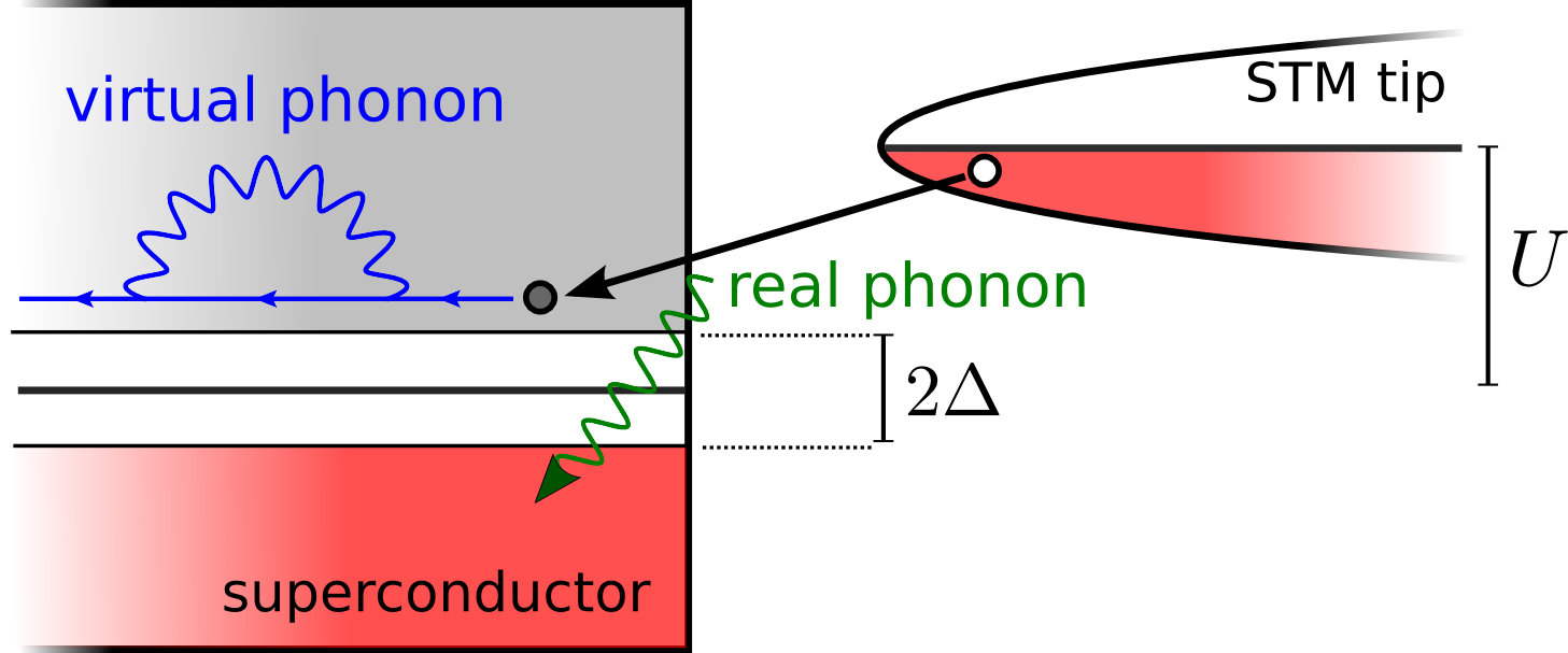
Figure 1: Illustration of the inelastic tunneling processes from a sharp tip (right) into a superconductor (left) in real space. Filled states are shown in red colour with energy along the vertical axis. The inelastic tunneling process is accompanied by the excitation of real phonons (green).

In this work, we determine experimentally and analyze theoretically the tunneling conductance of Pb that is affected by the coupling to real phonons via inelastic tunneling and virtual phonons via many-body renormalizations. Comparing the two approaches to determine $\alpha^{2}F(\omega)$ on the same sample with the same tip of a low temperature STM, we show that interpreting tunneling spectra of superconductors via the McMillan inversion algorithm (and thus solely by its elastic contribution) can be an incomplete description. We demonstrate that inelastic contributions to the tunneling current can, in general, be of the same order as the elastic contribution. We show that we can understand experimental STM data from Pb tunneling in the normal and superconducting state, taking into account both elastic and inelastic tunneling processes. The combined analysis of elastic and inelastic tunneling processes is important to correctly identify fingerprints of the relevant interactions in the electronic DOS and to identify the pairing glue for superconductivity. This is essential for conventional superconductors, such as Pb, but is expected to be even more important for unconventional pairing states, where an electronic pairing interaction is expected to fundamentally change its character upon entering the superconducting state.

We start with experimental data for STM measurements on lead. Measurements were performed with a home-build Joule-Thomson low-temperature STM (JT-STM)Lei1 at temperatures about 0.8 K. The JT-STM contains a magnet which allows to suppress superconductivity. In order to ensure that there is no significant inelastic signal of the tip at $\left|U\right|<15\text{ mV}$, we use a chemically etched tungsten tip, known to have a weak electron-phonon coupling McMillan1968tungsten . The highly n-doped Si(111) crystals were carefully degassed at 700 °C for several hours and then flashed to 1150 °C for 30 seconds to remove the native oxide. Lead was evaporated at room temperature from a Knudsen cell with a nominal thickness of 19 monolayers (ML). After deposition the samples were immediately transferred to the cryogenic STM. In agreement with previous studies Brun ; Eom2006 ; Altfeder1997 , flat-top, wedge-like islands of local thickness around 30ML were observed (see Fig. 2), i.e. extended 3D islands appear on top of a metallic wetting layer (WL) . The islands are Pb single crystals with their $\langle 111\rangle$ axis perpendicular to the substrate Eom2006 ; Weitering92 ; Jalochowski82 . The first (second) derivative of the tunneling current $dI/dU$ ($d^{2}I/dU^{2}$) of the islands was measured using a lock-in amplifier with a modulation voltage of $U_{\text{mod}}=439\,\mathrm{\mu V}$.

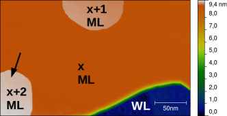
Figure 2: STM topography of Pb on Si(111) ($300\times 175\,\mathrm{nm^{2}},\ 1\,\mathrm{V},\ 1\,\mathrm{nA}$). The thickness of the island was determined to $x\approx$ 30 monolayers.

While the electrons in the $\approx 30$ML Pb film on Si have quantized $k_{z}$ leading to the flat island growth, the phonon DOS of the finite thickness films is rather similar to that of bulk Pb as indicated by first principle calculations Heid2013 ; Heid2010 . As a first measurement, we therefore determine $\alpha^{2}F_{\text{tun}}(\omega)$ of lead directly with ITS in the normal state. Pb islands were forced to the normal state by applying a magnetic field of 1T normal to the sample plane. Since the sample is in the normal state, no renormalization of the BCS density of states near the Fermi energy due to virtual phonons arises. Thus renormalization effects by virtual phonons can be neglected in $d^{2}I/dU^{2}$ and experimental features in $d^{2}I/dU^{2}$ correspond to inelastic tunneling. Fig. 3 shows the measured $d^{2}I/dU^{2}$ spectrum clearly revealing the two characteristic phonon peaks that are also seen in the Eliashberg function $\alpha^{2}F(\omega)$ determined by Ref. McMillan65 . Below we show explicitly that in the normal state $d^{2}I/dU^{2}$ is proportional to $\alpha^{2}F_{\text{tun}}(e\,U)$. These peaks at $U=$ 4.05 mV$\approx\omega_{t}$ and $U\approx$ 8.3 mV$\approx\omega_{l}$ (FWHM $\gamma_{t}=1.076$meV and $\gamma_{l}=0.60$meV) coincide with the energies of the transversal and longitudinal van Hove singularities in the phonon DOS of lead Heid2010 ; Brockhouse62 . The additional peak at $U\approx$ 12.5 mV can be explained by tunneling processes via two-phonon emission .

The key implication from Fig. 3 for the superconducting state is, however, that we must include inelastic contributions to the superconducting tunneling spectrum in a consistent fashion. Before we present our experimental data of the superconducting state, we summarize the theoretical description of the tunneling conductance in the superconducting state including inelastic contributions.

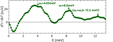
Figure 3: Second derivative $d^{2}I/dU^{2}\sim\alpha^{2}F_{\text{tun}}(eU)$ measured in the normal conducting state ($T=0.8$ K, $B=1$ T).

The Hamiltonian $\mathcal{H}=\mathcal{H}_{0}+\mathcal{H}_{\text{t}}$ used in our analysis of the combined substrate and tip consists of free electrons in the tip and electrons interacting with phonons in the substrate (we set $\hbar=1$):

$$\mathcal{H}_{0} =\sum_{\textbf{{p}},\sigma}\epsilon_{\textbf{{p}}}^{T}c_{\textbf{{p}},\sigma}^{\dagger}c_{\textbf{{p}},\sigma}+\sum_{\textbf{{k}},\sigma}\epsilon_{\textbf{{k}}}^{S}c_{\textbf{{k}},\sigma}^{\dagger}c_{\textbf{{k}},\sigma}+\sum_{\textbf{{q}},\mu}\omega_{\textbf{{q}},\mu}a_{\textbf{{q}},\mu}^{\dagger}a_{\textbf{{q}},\mu}$$

$$\hskip 8.53581pt+\frac{1}{\sqrt{V_{S}}}\sum_{{\textbf{{k}},\textbf{{k}}^{\prime}\atop\sigma,\mu}}\alpha_{\textbf{{k}}-\textbf{{k}}^{\prime},\mu}c_{\textbf{{k}},\sigma}^{\dagger}c_{\textbf{{k}}^{\prime},\sigma}\phi_{\textbf{{k}}-\textbf{{k}}^{\prime},\mu}\,.$$ (1)

Here, $\phi_{\textbf{{q}},\mu}=a_{\textbf{{q}},\mu}+a_{-\textbf{{q}},\mu}^{\dagger}$ is proportional to the lattice displacement, where $a_{\textbf{{q}},\mu}$ is the the phonon annihilation operator for momentum q and phonon-branch $\mu$ and with dispersion $\omega_{\textbf{{q}},\mu}$. $c_{\textbf{{k}}/\textbf{{p}},\sigma}^{\dagger}$ are the electron annihilation operators for the two subsystems: The tip (quasi-momentum p, dispersion $\epsilon_{\textbf{{p}}}^{T}$ and volume $V_{T}$) and the superconductor (quasi-momentum k, dispersion $\epsilon_{\textbf{{k}}}^{S}$ and volume $V_{S}$). For the latter we include the electron-phonon coupling $\alpha_{\textbf{{k}}-\textbf{{k}}^{\prime},\mu}$ that gives rise to superconductivity. The electron-phonon interaction in the tip is assumed to be small. In addition, the tunneling part of the Hamiltonian includes elastic and inelastic tunneling processes Taylor91 ; BennethDuke68 :

$$\mathcal{H}_{\text{t}} =\frac{1}{\sqrt{V_{T}V_{S}}}\sum_{{\textbf{{k}},\textbf{{p}}\atop\sigma}}T_{\textbf{{k}},\textbf{{p}}}c_{\textbf{{k}},\sigma}^{\dagger}c_{\textbf{{p}},\sigma}+\text{h.c.}\,,$$ (2)

$$T_{\textbf{{k}},\textbf{{p}}} =T_{\textbf{{k}},\textbf{{p}}}^{\text{e}}+\frac{1}{\sqrt{V_{S}}}\sum_{\textbf{{q}},\mu}T_{\textbf{{k}},\textbf{{p}},\textbf{{q}},\mu}^{\text{i}}\alpha_{\textbf{{q}},\mu}\phi_{\textbf{{q}},\mu}+\mathcal{O}(\phi_{\textbf{{q}},\mu}^{2})\,.$$

The first term of the tunneling amplitude $T_{\textbf{{k}},\textbf{{p}}}$ describes the elastic tunneling part, the second term corresponds to electron transitions via the emission/absorption of phonons, see Fig. 1. It is proportional to the bulk electron-phonon coupling $\alpha_{\textbf{{q}},\mu}$ Taylor91 . There can also be processes with a higher number of phonons, which will be discussed later.

In order to determine the tunneling current we assume that the DOS of the tip is constant $\nu_{T}(\omega)\approx\nu_{T}^{0}$ and that the tunneling amplitudes are independent of momenta and phonon branches $T_{\textbf{{k}},\textbf{{p}}}^{\text{e}}=t^{\text{e}}$ and $T_{\textbf{{k}},\textbf{{p}},\textbf{{q}},\mu}^{\text{i}}=t^{\text{i}}$, which is a reasonable approximation for STM Giamarchi2011 . Then, to leading order in $t^{\text{e}}$, the differential conductance gives the well known result Bardeen61 ; Cohen62 ; MahanBook

$$\sigma^{\text{e}}(U)=\frac{dI^{\text{e}}}{dU} =-e\sigma_{0}\int_{-\infty}^{\infty}d\omega\,n_{F}^{\prime}(\omega+eU)\tilde{\nu}_{S}(\omega).$$ (3)

In the limit that $T$ is smaller than the electronic energy scales, the conductance is just proportional to the the normalized electron DOS $\tilde{\nu}_{S}(\omega)=\nu_{S}(\omega)/\nu_{S}^{0}$, where $\nu_{S}^{0}$ is the normal state DOS of the superconductor at the Fermi level. The conductance constant is given by $\sigma_{0}=4\pi e^{2}\left|t^{\text{e}}\right|^{2}\nu_{T}^{0}\nu_{S}^{0}$ and $n_{F}$ is the Fermi function. In the normal state, $\tilde{\nu}_{S}(\omega)$ is essentially constant for small applied voltages and the second derivative of the elastic current vanishes, as discussed above. In the superconducting state, the opening of the superconducting gap and the excitation of virtual phonons lead to the mentioned fingerprints of superconductivity and the pairing glue in the elastic tunneling spectrum. Below we determine these structures from the solution of the nonlinear Eliashberg equations for given $\alpha^{2}F(\omega)$ and compare with our STM experiments.

The inelastic contribution to the differential conductance $\sigma^{\text{i}}(U)=\frac{dI^{\text{i}}}{dU}$ due to the excitation of single real phonons is for $U>0$ given by the convolution

$$\sigma^{\text{i}}(U)=\sigma_{0}\frac{\left|t^{\text{i}}\right|^{2}}{\left|t^{\text{e}}\right|^{2}\nu_{S}^{0}}\int_{-\infty}^{\infty}d\omega\,\alpha^{2}F_{\text{tun}}^{T}(eU+\omega)\tilde{\nu}_{S}(\omega)n_{F}(\omega)\,.$$ (4)

in the limit that the thermal phonons can be neglected $T\ll\omega_{D}$. The function $\alpha^{2}F_{\text{tun}}^{T}(x)=-\int_{-\infty}^{\infty}dy\,\alpha^{2}F_{\text{tun}}(y)n_{F}^{\prime}(y-x)$ is a thermally broadened version of the weighted phonon DOS $\alpha^{2}F_{\text{tun}}(\omega)=\frac{\nu_{S}^{0}}{V_{S}}\sum_{\textbf{{q}},\mu}\left|\alpha_{\textbf{{q}},\mu}\right|^{2}\delta(\omega-\omega_{\textbf{{q}},\mu})$ that is closely related to the Eliashberg function $\alpha^{2}F(\omega)=\frac{1}{\nu_{S}^{0}V_{S}^{2}}\sum_{\textbf{{k}},\textbf{{k}}^{\prime},\mu}\left|\alpha_{\textbf{{k}}-\textbf{{k}}^{\prime},\mu}\right|^{2}\delta(\omega-\omega_{\textbf{{k}}-\textbf{{k}}^{\prime},\mu})\delta(\epsilon_{\textbf{{k}}}^{S})\delta(\epsilon_{\textbf{{k}}^{\prime}}^{S})$. Both have similar features but can differ in fine-structure and amplitude.

The result (6) is the generalization of the current in the normal state, where $\frac{d^{2}I^{\text{i}}}{dU^{2}}\bigr{|}_{\text{NC}}\sim\text{sign}(U)\,\alpha^{2}F_{\text{tun}}(e\left|U\right|)$ is proportional to the weighted DOS of the phonons (or other collective excitations of the system), see Ref. BennethDuke68 ; Taylor91 ; KirtleyScalapino1990 ; Xiao1994 . It naturally explains the results of Fig. 3 or the recent STM measurements on Pb Schackert15 . Our measurement further allows for an estimate of the inelastic tunneling amplitude $t^{\text{i}}\approx t^{\text{e}}/D$, which is inversely proportional to the characteristic energy scale of the off-shell electrons involved in the tunneling process. The normal state elastic conductance $\sigma^{\text{e}}(U)\approx\sigma_{0}$ is not energy dependent for the applied biases $U$ and we emphasize that all spectra within this paper are normalized to $\sigma_{0}=\sigma(0)=\sigma^{\text{e}}(0)$ to point out the existence of inelastic tunneling contributions. The change in the conductance from 0 to 10 mV seen in Fig. 4a) is purely due to the inelastic tunneling. This leads to the condition $\sigma^{\text{i}}(10\,\text{mV})\approx 12\%\,\sigma_{0}$, where $\sigma(0)=\sigma_{0}$ is the purely elastic contribution at zero bias. Using the widely accepted Eliashberg function $\alpha^{2}F(\omega)$ and the experimental DOS for lead Gold60 , we can estimate for the characteristic off-shell electronic energy to be $D\approx 240\,\text{meV}$. Below, we will see that elastic and inelastic contributions to the fine-structure turn out to be comparable in magnitude.

In the superconducting state, the inelastic contribution Eq.(6) has its major contribution slightly below the energy of the phonon peaks shifted by the gap $\Delta$. Since inelastic tunneling opens additional channels to the conductance, it will lead to positive contributions to $d^{2}I/dU^{2}$ at positive bias. Elastic contributions are of opposite sign (see (3)). Thus, pronounced peaks in the second derivative of the tunneling current due to real phonons are followed by dips of same amplitude due to virtual phonons (for details see discussion of a single phonon mode in the Supplementary Material). As we will see below, we find exactly these features in the tunneling current for the STM experiment on lead.

Tunneling processes with a higher number of excited phonons will give similar terms as in (6) with higher convolutions of the Eliashberg-function such as $\alpha^{4}F_{\text{tun}}^{2}(\omega)=\int d\omega^{\prime}\alpha^{2}F_{\text{tun}}(\omega-\omega^{\prime})\alpha^{2}F_{\text{tun}}(\omega^{\prime})$ and one can formally absorb this contribution in a redefinition of $\alpha^{2}F_{\text{tun}}$ (see Supplementary Material).

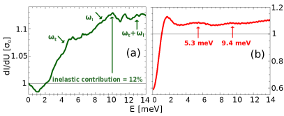
Figure 4: Differential conductance $dI/dU$ in the normal (a) and superconducting (b) state measured on the island marked by arrow in Fig. 2. The curves are normalized to the zero bias conductance $\sigma(0)$ in the normal state.

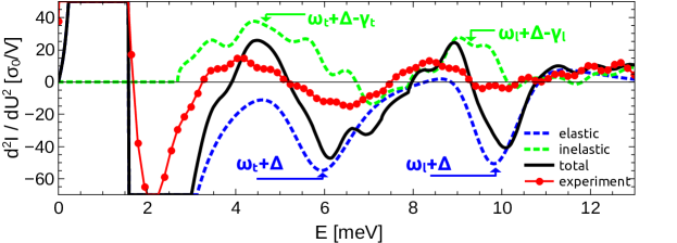
Figure 5: Comparison of experimental data (red) and theoretical prediction in the superconducting state: Calculated elastic (blue), inelastic (green) and total (black) contribution to $d^{2}I/dU^{2}$ (the elastic current is convoluted with a Gaussian function with standard deviation $\sigma=0.31\text{ meV}$ simulating the experimental broadening due to the modulation voltage of the lock-in technique). Characteristic peak-dip features around the zero axis can only be explained taking into account elastic and inelastic channels ($I^{\text{tot}}=I^{\text{el}}+I^{\text{inel}}$).

Without magnetic field, the islands are in the superconducting state. As the local thickness of the islands (30ML $\approx$ 10 nm) is significantly smaller than the bulk coherence length of lead (83 nm Kittel2005 ), the superconducting gap is not fully developed Brun ; Eom2006 ; Nishio2006 ; Nishio2008 ; Qin2009 ; Garcia2011 ; Bose2010 , which implies that the spectral weight of the coherence peaks is accordingly smaller (see Fig. 4b) ). Besides the Bogoliubov quasiparticle peak one clearly observes fine structures in the spectrum of the conductance around $U\approx$ 5.3 mV and $U\approx$ 9.4 mV. These energies correspond to the van Hove singularities in the phonon DOS $F(\omega)$ of lead shifted by the gap $\Delta\approx 1.2\text{ meV}$ clearly indicating electron-phonon interaction induced effects. Furthermore, the typical $\omega/\sqrt{\omega^{2}-\Delta^{2}}$ behavior in the BCS DOS is altered by the emergence of inelastic contributions at biases $V_{0}>5mV$ . This is in contrast to previous measurements on planar tunneling junctions of lead  Giaever62 ; Schrieffer63 ; Rowell62 ; Rowell63 ; RowellinParks ; Giaever74 , where these inelastic contributions were about one order of magnitude smaller Rowell69 than in our present experiment. The reason is that inelastic tunneling events are enhanced in STM geometries, if compared to planar tunneling junctions, because the momentum conservation for momenta parrallel to the surface are less restrictive Giamarchi2011 .
Let us now investigate the second derivative of the tunneling current in the superconducting state, which is significantly more sensitive to the fine structure induced by the electron-phonon interaction. For the theoretical spectrum, we first use a parameterization of the $\alpha^{2}F(\omega),\mu^{*}$ from McMillan and Rowell McMillan65 ; Galkin to solve the Eliashberg equations numerically Schmalian96 to obtain the lead DOS $\nu_{S}(\omega)$ in the superconducting state. The elastic contribution to the second derivative is then easily calculated using Eq. (3). For the inelastic contribution we use the $\alpha^{2}F_{\text{tun}}(\omega)$ function (without the negative dip at small voltages $U<2$ mV that comes from a zero bias anomaly) and the calculated DOS $\nu_{S}(\omega)$ to determine the convolution in Eq. (6), where the usage of the measured $\alpha^{2}F_{\text{tun}}(\omega)$ function automatically includes two-phonon processes and yields the correct amplitude for the inelastic tunneling current. Note, that the rapid wiggels on top of the calculated inelastic curve are due to noise of the input data of the calculations, i.e. the experimental inelastic spectrum in the normal state. This noise is caused by residual mechanical vibrations on the level of 300 fm. When convoluting the noisy experimental spectra with the DOS for the calculation of the inelastic contribution in the superconducting state, certain frequencies of the noise are amplified and show up as small wiggels. Finally, we convoluted the elastic part with a Gaussian distribution (standard deviation $\sigma=310\mu\text{eV}$ corresponding to an energy resolution of $744\mu\text{eV}$), describing the experimental broadening due to the modulation voltage of the lock-in detection Klein73 .

In Fig. 5 we compare the experimental data with the theoretical prediction of the elastic, inelastic and total contributions of the second derivative of the current. The experimental data show peak-dip features around the zero axis at positions that correspond to the characteristic longitudinal and transversal phonon energies $\omega_{\text{t}/\text{l}}$ shifted by the gap $\Delta\approx 1.2\text{ meV}$. For both features there is a positive peak at $\approx\omega_{t,l}+\Delta-\gamma_{t,l}$ of the same magnitude as the corresponding dip at $\omega_{t,l}+\Delta$, where $\gamma_{t,l}$ are the half-widths of the phonon peaks observed in Fig. 3. This is in contrast to the theoretical elastic $d^{2}I^{\text{e}}/dU^{2}\sim\nu^{\prime}(-eU)$ curve, which only shows the typical dips around $\Delta+\omega_{\text{t/l}}$ predicted by the Eliashberg theory. We note that conventional Eliashberg theory can also have positive peaks, but the following dip will always be significantly more pronounced (see also Fig. 4 in the Supplementary material). Therefore, the observed peak-dip features cannot be explained by pure elastic tunneling. However, the measured spectrum both in the normal and in the superconducting state can naturally be explained when we combine inelastic and elastic contributions. As can be seen, the total theoretical conductance $d^{2}I^{\text{tot}}/dU^{2}$ consisting of elastic and inelastic channels fits the experimental peak-dip features much better at the correct energies.

In summary, we demonstrated experimentally and theoretically that in normal conducting Pb islands it is possible to directly measure the collective bosonic excitation spectrum, here phonons, using STM. In the normal conducting state, the obtained $d^{2}I/dU^{2}$ spectra is proportional to the weighted phonon DOS $\alpha^{2}F_{\text{tun}}(\omega)$ and higher convolutions thereof. This is different in the superconducting state of Pb. Here, the obtained second derivative $d^{2}I/dU^{2}=d^{2}I^{\text{e}}/dU^{2}+d^{2}I^{\text{i}}/dU^{2}$ spectra are a composition of elastic and inelastic tunneling processes with fine structures in the same energy regime. While the elastic part shows phonon features coming from self energy corrections (exchange of virtual phonons) that appear mainly as dips in the second derivative of the tunneling current, the inelastic part shows features of $\alpha^{2}F_{\text{tun}}(\omega)$ shifted by the superconducting gap $\Delta$ giving rise to additional peak features of the same amplitude at lower energies (excitation of real phonons). A rather unique signature of these inelastic contributions are peak-dip features in $d^{2}I/dU^{2}$ around zero at $\Delta+\omega_{\text{ph}}$ in the superconducting state. Those cannot be explained by only taking into account the elastic part $d^{2}I^{\text{e}}/dU^{2}$. For this reason, the neglect of inelastic processes in STM experiments in general not justified. Hence, when analyzing STM tunneling spectra via the McMillan inversion algorithm McMillan65 ; Galkin , that gives the purely elastic contribution, one should carefully subtract the inelastic contributions from the experimental tunneling current. Otherwise grossly incorrect conclusions about the pairing glue would be deduced from the tunneling spectrum.

Having found out experimentally and theoretically how elastic and inelastic tunneling can be disentangled for STM in conventional superconductors, the approach can be generalized to the investigation of corresponding bosonic structures in high temperature superconductors such as cuprates and iron pnictides in the future. A crucial difference to the phononic pairing glue is that in case of electronic pairing, the bosonic spectrum undergoes dramatic reorganization below $T_{c}$ in form of a sharp resonance in the dynamic spin excitation spectrum RossatMignod1991 ; Mook1993 ; Fong1999 ; Christianson2008 ; Inosov2010 ; Abanov2001 . Our results imply that great care must be taken in the proper interpretation of the tunneling spectra of these systems and that real and virtual bosonic excitations must be disentangled in a fashion similar to our analysis for lead.

Supplemental Material

Appendix A Derivation of the tunnel current

A.1 Peturbative approach

The tunneling current is given by elementary charge times the change of the number of electrons $n_{S}=\sum_{\textbf{{k}},\sigma}c_{\textbf{{k}},\sigma}^{\dagger}c_{\textbf{{k}},\sigma}$ in the superconductor

$$I =-e\frac{d}{dt}\text{tr}\bigl{[}\rho(t)n_{S}\bigr{]}/\text{tr}[\rho(t)]$$

$$=ie\,\text{tr}\bigl{(}\rho_{0}\bigl{[}n_{S}(t),\mathcal{H}(t)\bigr{]}\bigr{)}/\text{tr}[\rho_{0}]$$

$$=ie\langle\,{\bigl{[}n_{S}(t),\mathcal{H}(t)\bigr{]}}\,\rangle$$ (5)

where $\rho(t)=U(t,\infty)\rho_{0}U^{\dagger}(t,-\infty)$ is the time-dependent density matrix and $\langle\,{\ldots}\,\rangle_{0}=\langle\,{\rho_{0}\ldots}\,\rangle=\langle\,{e^{-\beta\mathcal{H}}\ldots}\,\rangle$ is the expectation value of the system in thermal equilibrium with density matrix $\rho_{0}=e^{-\beta\mathcal{H}}$. A suitable formalism to calculate the current (5) is the Keldysh Green function method (we follow the notation of Ref. [Keldyshbook, ]). The corresponding Keldysh action of the Hamiltonian (without bias voltage) employed in the main text of the paper is given by

$$S =S_{0}+S_{\text{t}}$$ (6)

$$S_{0} =\int_{\mathcal{C}}dt\,\sum_{\textbf{{p}},\sigma}\bar{c}_{\textbf{{p}},\sigma}(t)(i\partial_{t}-\epsilon_{\textbf{{p}}}^{T})c_{\textbf{{p}},\sigma}(t)$$

$$\hskip 8.53581pt+\int_{\mathcal{C}}dt\,\sum_{\textbf{{k}},\sigma}\bar{c}_{\textbf{{k}},\sigma}(t)(i\partial_{t}-\epsilon_{\textbf{{k}}}^{S})c_{\textbf{{k}},\sigma}(t)$$

$$\hskip 8.53581pt+\int_{\mathcal{C}}dt\,\sum_{\textbf{{q}},\mu}\bar{a}_{\textbf{{q}},\mu}(t)(i\partial_{t}-\omega_{\textbf{{q}},\mu})a_{\textbf{{q}},\mu}(t)$$

$$\hskip 8.53581pt-\frac{1}{\sqrt{V_{S}}}\int_{\mathcal{C}}dt\,\sum_{\textbf{{k}},\textbf{{k}}^{\prime}\atop\sigma,\mu}\alpha_{\textbf{{k}}-\textbf{{k}}^{\prime},\mu}\bar{c}_{\textbf{{k}},\sigma}(t)c_{\textbf{{k}}^{\prime},\sigma}(t)\phi_{\textbf{{k}}-\textbf{{k}}^{\prime},\mu}(t)$$

$$S_{\text{t}} =-\frac{1}{\sqrt{V_{S}V_{T}}}\int_{\mathcal{C}}dt\,\sum_{\textbf{{k}},\textbf{{p}}}T_{\textbf{{k}},\textbf{{p}}}^{\text{e}}\bar{c}_{\textbf{{k}},\sigma}(t)c_{\textbf{{p}},\sigma}(t)$$

$$\hskip 8.53581pt-\frac{1}{V_{S}\sqrt{V_{T}}}\int_{\mathcal{C}}dt\,\sum_{\textbf{{k}},\textbf{{p}},\textbf{{q}}\atop\sigma,\mu}T_{\textbf{{k}},\textbf{{p}},\textbf{{q}},\mu}^{\text{i}}\,\alpha_{\textbf{{q}},\mu}\bar{c}_{\textbf{{k}},\sigma}(t)c_{\textbf{{p}},\sigma}(t)\phi_{\textbf{{q}},\mu}(t)$$

$$\quad+\text{h.c.}$$

where as usual we defined the phonon displacement field $\phi_{\textbf{{q}},\mu}=a_{\textbf{{q}},\mu}+a_{-\textbf{{q}},\mu}^{\dagger}$. In order to derive the $I-U$ characteristic of the system we have to apply a finite voltage $eU=\mu_{S}-\mu_{T}$, which can be done easily by the substitution $c_{\textbf{{p}},\sigma}(t)\rightarrow e^{-i\mu_{T}t}c_{\textbf{{p}},\sigma}(t)$ and $c_{\textbf{{k}},\sigma}(t)\rightarrow e^{-i\mu_{S}t}c_{\textbf{{k}},\sigma}(t)$. The dispersion energies of the tip $\epsilon_{\textbf{{p}}}^{T}\rightarrow\xi_{\textbf{{p}}}^{T}=\epsilon_{\textbf{{p}}}^{T}-\mu_{T}$ and superconductor $\epsilon_{\textbf{{k}}}^{S}\rightarrow\xi_{\textbf{{k}}}^{S}=\epsilon_{\textbf{{k}}}^{S}-\mu_{T}$ are now measured relative to their chemical potentials and this leads to a time dependence of the tunneling matrix elements $T^{\text{e}}\rightarrow T^{\text{e}}e^{ieUt},T^{\text{i}}\rightarrow T^{\text{i}}e^{ieUt}$ in the tunneling part $S_{\text{t}}$ of the action.

We build up our perturbation theory by rewriting $\langle\,{\ldots}\,\rangle=\int D[\bar{c},c]D[\bar{a},a]\ldots e^{iS}=\langle\,{e^{iS_{\text{t}}}\ldots}\,\rangle_{0}$ with the unperturbed expectation value $\langle\,{\ldots}\,\rangle_{0}=\int D[\bar{c},c]D[\bar{a},a]\ldots e^{iS_{0}}$. The corresponding unperturbed propagators are then given in the $R,A,K$ basis (also known as Larkin-Ovchinnikov Representation)

$$\hat{G}_{\textbf{{k}}/\textbf{{p}}}(t,t^{\prime}) =-i\langle\,{\left(\begin{matrix}c_{\textbf{{k}}/\textbf{{p}},\sigma}^{1}(t)\\ c_{\textbf{{k}}/\textbf{{p}},\sigma}^{2}(t)\end{matrix}\right)\left(\begin{matrix}c_{\textbf{{k}}/\textbf{{p}},\sigma}^{1}(t^{\prime})\\ c_{\textbf{{k}}/\textbf{{p}},\sigma}^{2}(t^{\prime})\end{matrix}\right)^{\dagger}}\,\rangle_{0}$$

$$=\left(\begin{matrix}G_{\textbf{{k}}/\textbf{{p}}}^{R}(t,t^{\prime})&G_{\textbf{{k}}/\textbf{{p}}}^{K}(t,t^{\prime})\\ 0&G_{\textbf{{k}}/\textbf{{p}}}^{A}(t,t^{\prime})\end{matrix}\right)$$

$$\hat{D}_{\textbf{{q}},\mu}(t,t^{\prime}) =-i\langle\,{\left(\begin{matrix}\phi_{\textbf{{q}},\mu}^{\text{cl}}\\ \phi_{\textbf{{q}},\mu}^{\text{q}}\end{matrix}\right)\left(\begin{matrix}\phi_{-\textbf{{q}},\mu}^{\text{cl}}\\ \phi_{-\textbf{{q}},\mu}^{\text{q}}\end{matrix}\right)^{\dagger}}\,\rangle_{0}$$

$$=\left(\begin{matrix}D_{\textbf{{q}},\mu}^{K}(t,t^{\prime})&D_{\textbf{{q}},\mu}^{R}(t,t^{\prime})\\ D_{\textbf{{q}},\mu}^{A}(t,t^{\prime})&0\end{matrix}\right)$$ (7)

where the retarded propagators are given in energy representation $f(\omega)=\int_{-\infty}^{\infty}dtf(t)e^{i\omega t}$ as

$$G_{\textbf{{k}}}^{R}(\omega) =\begin{matrix}\includegraphics[width=22.76219pt]{GS.pdf}\end{matrix}=\frac{Z_{\textbf{{k}}}^{R}(\omega)\,\omega+\xi_{\textbf{{k}}}^{S}}{\bigl{[}Z_{\textbf{{k}}}^{R}(\omega)\,\omega\bigr{]}^{2}-\bigl{[}\xi_{\textbf{{k}}}^{S}\bigr{]}^{2}-\Phi_{\textbf{{k}}}^{R}(\omega)^{2}}$$

$$F_{\textbf{{k}}}^{R}(\omega) =\begin{matrix}\includegraphics[width=22.76219pt]{FS.pdf}\end{matrix}=\frac{-\Phi_{\textbf{{k}}}^{R}(\omega)}{\bigl{[}Z_{\textbf{{k}}}^{R}(\omega)\,\omega\bigr{]}^{2}-\bigl{[}\xi_{\textbf{{k}}}^{S}\bigr{]}^{2}-\Phi_{\textbf{{k}}}^{R}(\omega)^{2}}$$

$$G_{\textbf{{p}}}^{R}(\omega) =\begin{matrix}\includegraphics[width=22.76219pt]{GT.pdf}\end{matrix}=\frac{1}{\omega-\xi_{\textbf{{p}}}^{S}+i0}$$

$$D_{\textbf{{q}},\mu}^{R}(\omega) =\begin{matrix}\includegraphics[width=22.76219pt]{DP.pdf}\end{matrix}=\frac{2\omega_{\textbf{{q}},\mu}}{(\omega+i0)^{2}-\omega_{\textbf{{q}},\mu}^{2}}$$ (8)

For the superconductor, we use the known framework of Eliashberg theory. Therefore, $Z_{\textbf{{k}}}^{R}=1-\frac{\Sigma_{\textbf{{k}}}^{R}(\omega)-\Sigma_{-\textbf{{k}}}^{A}(-\omega)}{2\omega}$ is the renormalization function of the lead superconductor $S$ and $\Sigma_{\textbf{{k}}}^{R/A}(\omega)=\Sigma_{\textbf{{k}}}(\omega\pm i0)$ is the phonon-induced normal self-energy, see Fig. 6. We neglected the correction of the pure dispersion $\xi_{\textbf{{k}}}^{S}$ due to the coupling to the phonons, because it will basically just give an unimportant shift of the chemical potential and can be assumed to be incorporated in the electronic dispersion already from the beginning. The anomalous self-energy $\Phi_{\textbf{{k}}}^{R}(\omega)=\Phi_{\textbf{{k}}}(\omega+i0)$ is depicted in Fig. 6 and we also gave the expression for the anomalous propagator $F_{\textbf{{k}}}^{R}(\omega)$, even tough we will only need the normal particle propagator (since in the NIS-junction there is no Josephson effect). We neglect the renormalization of the phonon spectrum due to the interaction with the electrons, which could be incorporated easily by a phonon self-energy that would just lead to a small broadening and modification of the phonon spectral weight. The effect of the Coulomb interaction between the fermions is as usual incorporated using a Coulomb pseudopotential $\mu^{*}$.

Figure 6: Normal and anomalous self-energy due to electron-phonon interaction that appear in the Eliashberg-theory.

Since we consider the sub-systems $S$ and $T$ to be in thermal equilibrium, the Keldysh propagators have the simple structure

$$G_{\textbf{{k}}/\textbf{{p}}}^{K}(\omega) =\bigl{[}1-2n_{F}(\omega)\bigr{]}\,\underbrace{\bigl{[}G_{\textbf{{k}}/\textbf{{p}}}^{R}(\omega)-G_{\textbf{{k}}/\textbf{{p}}}^{A}(\omega)\bigr{]}}_{-2\pi iA_{\textbf{{k}}/\textbf{{p}}}(\omega)}\,,$$

$$D_{\textbf{{q}},\mu}^{K}(\omega) =\bigl{[}1+2n_{B}(\omega)\bigr{]}\,\underbrace{\bigl{[}D_{\textbf{{q}},\mu}^{R}(\omega)-D_{\textbf{{q}},\mu}^{A}(\omega)\bigr{]}}_{-2\pi i\bigl{[}A_{\textbf{{q}},\mu}(\omega)-A_{\textbf{{q}},\mu}(-\omega)\bigr{]}}\,,$$ (9)

where $n_{F}(\omega)$ is the Fermi and $n_{B}(\omega)$ the Bose function with temperature $T$ and we defined the spectral weights $A_{\textbf{{k}}/\textbf{{p}}}(\omega),A_{\textbf{{q}},\mu}(\omega)$ of the electron and phonon systems. In our case $A_{\textbf{{q}},\mu}(\omega)=\delta(\omega-\omega_{\textbf{{q}},\mu})$. For completeness, we also give the explicit expressions for the greater/lesser Green functions

$$G_{\textbf{{k}}/\textbf{{p}}}^{>/<}(\omega) =-2\pi i\left\{\begin{matrix}1-n_{F}(\omega)\\ -n_{F}(\omega)\end{matrix}\right\}A_{\textbf{{k}}/\textbf{{p}}}(\omega)$$ (10)

$$D_{\textbf{{q}},\mu}^{>/<}(\omega) =-2\pi i\left\{\begin{matrix}1+n_{B}(\omega)\\ n_{B}(\omega)\end{matrix}\right\}\biggl{[}A_{\textbf{{q}},\mu}(\omega)-A_{\textbf{{q}},\mu}(-\omega)\biggr{]}$$

Following Eq. (5) it is easy to determine the explicit expression for the current

$$I =ie\langle\,{\sum_{\textbf{{k}},\textbf{{p}}}\left(\begin{matrix}c_{\textbf{{p}},\sigma}^{-}(t)\\ c_{\textbf{{k}},\sigma}^{-}(t)\end{matrix}\right)^{\dagger}\left(\begin{matrix}0&-[T_{\textbf{{k}},\textbf{{p}}}^{+}(t)]^{*}\\ T_{\textbf{{k}},\textbf{{p}}}^{-}(t)&0\end{matrix}\right)\left(\begin{matrix}c_{\textbf{{p}},\sigma}^{+}(t)\\ c_{\textbf{{k}},\sigma}^{+}(t)\end{matrix}\right)}\,\rangle$$

$$=ie\langle\,{\sum_{\textbf{{k}},\textbf{{p}}}\left(\begin{matrix}c_{\textbf{{p}},\sigma}^{-}(t)\\ c_{\textbf{{k}},\sigma}^{-}(t)\end{matrix}\right)^{\dagger}\left(\begin{matrix}0&-[T_{\textbf{{k}},\textbf{{p}}}^{+}(t)]^{*}\\ T_{\textbf{{k}},\textbf{{p}}}^{-}(t)&0\end{matrix}\right)\left(\begin{matrix}c_{\textbf{{p}},\sigma}^{+}(t)\\ c_{\textbf{{k}},\sigma}^{+}(t)\end{matrix}\right)e^{iS_{\text{t}}}}\,\rangle_{0}$$

$$\approx-e\langle\,{\sum_{\textbf{{k}},\textbf{{p}}}\left(\begin{matrix}c_{\textbf{{p}},\sigma}^{-}(t)\\ c_{\textbf{{k}},\sigma}^{-}(t)\end{matrix}\right)^{\dagger}\left(\begin{matrix}0&-[T_{\textbf{{k}},\textbf{{p}}}^{+}(t)]^{*}\\ T_{\textbf{{k}},\textbf{{p}}}^{-}(t)&0\end{matrix}\right)\left(\begin{matrix}c_{\textbf{{p}},\sigma}^{+}(t)\\ c_{\textbf{{k}},\sigma}^{+}(t)\end{matrix}\right)S_{\text{t}}}\,\rangle_{0}$$ (11)

where we defined the total tunneling matrix element $T_{\textbf{{k}},\textbf{{p}}}^{\pm}(t)=e^{ieUt}\bigl{[}T_{\textbf{{k}},\textbf{{p}}}^{\text{e}}+\sum_{\textbf{{q}},\mu}T_{\textbf{{k}},\textbf{{p}}}^{\text{e}}\alpha_{\textbf{{q}},\mu}\phi_{\textbf{{q}},\mu}^{\pm}(t)\bigr{]}$ (with phonon field $\phi^{\pm}$ on the upper/lower Keldysh contour) and in the end expanded in leading order of $T_{\textbf{{k}},\textbf{{p}}}$. Also, we defined the creation operators to be defined on the lower Keldysh contour (index $-$) and the annihilation operators on the upper Keldysh contour (index $+$), since the electron first has to leave one side before it can tunnel through the barrier to the other side. This time ordering can be conveniently expressed in Keldysh theory and we also assumed the phonons (field $\phi^{\pm}$) to be excited/absorbed on the same contour as the electrons on the superconductor $S$. The tunneling action can be written in a similar way as

$$S_{\text{t}} =-\int_{\mathcal{C}}dt\sum_{\textbf{{k}},\textbf{{p}}}\left(\begin{matrix}c_{\textbf{{p}},\sigma}(t)\\ c_{\textbf{{k}},\sigma}(t)\end{matrix}\right)^{\dagger}\left(\begin{matrix}0&[T_{\textbf{{k}},\textbf{{p}}}(t)]^{*}\\ T_{\textbf{{k}},\textbf{{p}}}(t)&0\end{matrix}\right)\left(\begin{matrix}c_{\textbf{{p}},\sigma}(t)\\ c_{\textbf{{k}},\sigma}(t)\end{matrix}\right)$$

$$=-\int\limits_{-\infty}^{\infty}dt\sum_{\textbf{{k}},\textbf{{p}}\atop\alpha=\pm}\alpha\,\left(\begin{matrix}c_{\textbf{{p}},\sigma}^{\alpha}(t)\\ c_{\textbf{{k}},\sigma}^{\alpha}(t)\end{matrix}\right)^{\dagger}\left(\begin{matrix}0&[T_{\textbf{{k}},\textbf{{p}}}^{\alpha}(t)]^{*}\\ T_{\textbf{{k}},\textbf{{p}}}^{\alpha}(t)&0\end{matrix}\right)\left(\begin{matrix}c_{\textbf{{p}},\sigma}^{\alpha}(t)\\ c_{\textbf{{k}},\sigma}^{\alpha}(t)\end{matrix}\right)$$ (12)

A.2 Elastic current

Performing the contractions in Eq. (11) we find the elastic current

$$I^{\text{e}}(U) =2e\int\limits_{-\infty}^{\infty}d\tau\,\frac{1}{V_{S}V_{T}}\sum_{\textbf{{k}},\textbf{{p}}}\left|T_{\textbf{{k}},\textbf{{p}}}^{\text{e}}\right|^{2}e^{ieU\tau}\,\sum_{\alpha=\pm}\alpha$$

$$\hskip 8.53581pt\bigl{[}G_{\textbf{{k}}}^{\alpha,-}(-\tau)G_{\textbf{{p}}}^{+,\alpha}(\tau)-G_{\textbf{{k}}}^{+,\alpha}(-\tau)G_{\textbf{{p}}}^{\alpha,-}(\tau)\bigr{]}$$

$$=-4e\int\limits_{-\infty}^{\infty}d\tau\,\frac{1}{V_{S}V_{T}}\sum_{\textbf{{k}},\textbf{{p}}}\left|T_{\textbf{{k}},\textbf{{p}}}^{\text{e}}\right|^{2}e^{ieU\tau}$$ (13)

$$\hskip 8.53581pt\bigl{[}\text{Im}\,G_{\textbf{{k}}}^{<}(-\tau)\text{Im}\,G_{\textbf{{p}}}^{R}(\tau)-\text{Im}\,G_{\textbf{{k}}}^{R}(-\tau)\text{Im}\,G_{\textbf{{p}}}^{<}(\tau)\bigr{]}$$

where we used the definition of the greater/lesser $G^{>/<}$ and time-ordered/anti-time-ordered Green function $G^{\mathcal{T}/\tilde{\mathcal{T}}}$, see Section E of the Supplementary Material. In the end, we used the known identities that relate $G^{\mathcal{T}/\tilde{\mathcal{T}}}$ to the greater, lesser, retarded and advanced propagators. In Fig. 7 we show the corresponding Feynman diagram for the elastic tunneling current for the leading order in the tunneling element. After transforming to Fourier space and inserting the explicit expressions of the propagators in thermal equilibrium, we find

$$I^{\text{e}}(U) =4\pi e\int\limits_{-\infty}^{\infty}d\omega\,\frac{1}{V_{S}V_{T}}\sum_{\textbf{{k}},\textbf{{p}}}\left|T_{\textbf{{k}},\textbf{{p}}}^{\text{e}}\right|^{2}$$ (14)

$$\hskip 8.53581pt\bigl{[}n_{F}(\omega)-n_{F}(\omega+eU)\bigr{]}A_{\textbf{{k}}}(\omega)A_{\textbf{{p}}}(\omega+eU)\,,$$

which is the usual expression for the elastic current in the Landauer-Büttinger transport theory assuming perfect quasiparticles $A_{\textbf{{k}}/\textbf{{p}}}(\omega)=\delta(\omega-\epsilon_{\textbf{{k}}/\textbf{{p}}}^{S/T})$.

The elastic conductance $G^{\text{e}}(U)=\frac{dI^{\text{e}}}{dU}$ will now be calculated using the usual approximation $T_{\textbf{{k}},\textbf{{p}}}^{\text{e}}=t^{\text{e}}=\text{const.}$ for small voltages $U\ll E_{F}\sim 1\text{ eV}$, which is a reasonable assumption for an STM Giamarchi2011, . Assuming the DOS of the tip system $\nu^{T}(\omega)=1/V_{T}\sum_{\textbf{{p}}}A_{\textbf{{p}}}(\omega)\approx\nu_{T}^{0}$ to be constant near the Fermi surface, we can then rewrite the elastic current (14) to be

$$I^{\text{e}}(U) =4\pi\nu_{T}^{0}e\left|t^{\text{e}}\right|^{2}\int_{-\infty}^{\infty}d\omega\,\bigl{[}n_{F}(\omega)-n_{F}(\omega+eU)\bigr{]}\nu_{S}(\omega)\,,$$ (15)

where we defined as usual the DOS of the superconductor as $\nu(\omega)=1/V_{S}\sum_{\textbf{{k}}}A_{\textbf{{k}}}(\omega)$. As it is well known, the elastic differential conductance is then given by

$$\frac{dI^{\text{e}}}{dU} =-4\pi\nu_{T}^{0}e^{2}\left|t^{\text{e}}\right|^{2}\int_{-\infty}^{\infty}d\omega\,n_{F}^{\prime}(\omega+eU)\nu_{S}(\omega)$$

$$=-\sigma_{0}\int_{-\infty}^{\infty}d\omega\,n_{F}^{\prime}(\omega+eU)\tilde{\nu}_{S}(\omega)$$ (16)

where we defined as the normalized DOS $\tilde{\nu}(\omega)=\nu(\omega)/\nu_{S}^{0}$ with $\nu_{S}^{0}$ as the DOS and $\sigma_{0}=4\pi\nu_{T}^{0}\nu_{S}^{0}e^{2}\left|t^{\text{e}}\right|^{2}$ as the elastic conductance in the normal state. For small temperatures ($T\ll E_{F}$ in the normal conductor or $T\ll\Delta$ in the superconductor with gap $\Delta$), such that $n_{F}^{\prime}(\epsilon)\approx-\delta(\epsilon)$, the elastic conductance simplifies to

$$\frac{dI^{\text{e}}}{dU} =4\pi\nu_{T}^{0}e^{2}\left|t^{\text{e}}\right|^{2}\nu(-eU)=\sigma_{0}\tilde{\nu}(-eU)\,,$$ (17)

and is then proportional to the normalized DOS $\tilde{\nu}(\omega)$ of the superconductor. The corresponding expression von $d^{2}I^{\text{e}}/dU^{2}$ can be computed easily from the expression (16).

Figure 7: Feynman diagrams for the elastic (left) and inelastic (right) tunneling current in leading order $T^{\text{e}},T^{\text{i}}$.

A.3 Inelastic current

The inelastic current can similarly be expressed by performing the contractions of (11) containing the phonon-fields and expressing the occurring propagators in terms of retarded, advanced, greater and lesser propagators

$$I^{\text{i}}(U) =2ie\int\limits_{-\infty}^{\infty}d\tau\,\frac{1}{V_{S}^{2}V_{T}}\sum_{\textbf{{k}},\textbf{{p}}\atop\textbf{{q}},\mu}\left|T_{\textbf{{k}},\textbf{{p}},\textbf{{q}},\mu}^{\text{i}}\alpha_{\textbf{{q}},\mu}\right|^{2}e^{ieU\tau}\sum_{\alpha=\pm}\alpha\biggl{[}G_{\textbf{{k}}}^{\alpha,-}(-\tau)G_{\textbf{{p}}}^{+,\alpha}(\tau)D_{\textbf{{q}},\mu}^{-,\alpha}(\tau)-G_{\textbf{{k}}}^{+,\alpha}(-\tau)G_{\textbf{{p}}}^{\alpha,-}(\tau)D_{\textbf{{q}},\mu}^{\alpha,+}(\tau)\biggr{]}$$

$$=4e\int\limits_{-\infty}^{\infty}d\tau\,\frac{1}{V_{S}^{2}V_{T}}\sum_{\textbf{{k}},\textbf{{p}}\atop\textbf{{q}},\mu}\left|T_{\textbf{{k}},\textbf{{p}},\textbf{{q}},\mu}^{\text{i}}\alpha_{\textbf{{q}},\mu}\right|^{2}e^{ieU\tau}\biggl{[}\text{Im}\,G_{\textbf{{k}}}^{<}(-\tau)\text{Im}\,G_{\textbf{{p}}}^{<}(\tau)\text{Im}\,D_{\textbf{{q}},\mu}^{R}(\tau)+\text{Im}\,G_{\textbf{{k}}}^{<}(-\tau)\text{Im}\,G_{\textbf{{p}}}^{R}(\tau)\text{Im}\,D_{\textbf{{q}},\mu}^{>}(\tau)$$

$$\hskip 199.16928pt-\text{Im}\,G_{\textbf{{k}}}^{R}(-\tau)\text{Im}\,G_{\textbf{{p}}}^{<}(\tau)\text{Im}\,D_{\textbf{{q}},\mu}^{<}(\tau)\biggr{]}$$ (18)

After going to Fourier space and inserting the corresponding electron and phonon propagators defined in Sec. A.1, we can finally rewrite the inelastic current as

$$I^{\text{i}}(U) =-4\pi e\int d\omega_{1}d\omega_{2}\frac{1}{V_{S}^{2}V_{T}}\sum_{\textbf{{k}},\textbf{{p}},\textbf{{q}}\atop\mu}\left|T_{\textbf{{k}},\textbf{{p}},\textbf{{q}},\mu}^{i}\alpha_{\textbf{{q}},\mu}\right|^{2}$$ (19)

$$\hskip 8.53581pt\biggl{[}A_{\textbf{{q}},\mu}(\omega_{1})A_{\textbf{{k}}}(\omega_{2})A_{\textbf{{p}}}(\omega_{2}-\omega_{1}+eU)\biggl{(}n_{F}(\omega_{2}-\omega_{1}+eU)n_{B}(\omega_{1})\bigl{[}1-n_{F}(\omega_{2})\bigr{]}-n_{F}(\omega_{2})\bigl{[}1+n_{B}(\omega_{1})\bigr{]}\bigl{[}1-n_{F}(\omega_{2}-\omega_{1}+eU)\bigr{]}\biggr{)}$$

$$\hskip 8.53581pt+A_{\textbf{{q}},\mu}(\omega_{1})A_{\textbf{{k}}}(\omega_{2})A_{\textbf{{p}}}(\omega_{2}+\omega_{1}+eU)\biggl{(}n_{F}(\omega_{2}+\omega_{1}+eU)\bigl{[}1+n_{B}(\omega_{1})\bigr{]}\bigl{[}1-n_{F}(\omega_{2})\bigr{]}-n_{F}(\omega_{2})n_{B}(\omega_{1})\bigl{[}1-n_{F}(\omega_{2}+\omega_{1}+eU)\bigr{]}\biggr{)}\biggr{]}$$

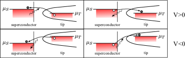
Figure 8: Inelastic tunneling processes for $V>0$ and $V<0$ via the emission/absorption of phonons.

The first/third term describes the tunneling of an electron from the tip to the superconductor via the absorption/excitation of a phonon and the second/fourth term the tunneling from the superconductor to the tip via a phonon excitation/absorption, see also Fig. 8. As in the elastic case, we apply the following simplifications: A constant inelastic vertex $T_{\textbf{{k}},\textbf{{p}},\textbf{{q}},\mu}^{\text{i}}=t^{i}$ and a constant DOS of the tip. Let us define the weighted DOS of the phonons in the superconductor as

$$\alpha^{2}F_{\text{tun}}(\omega) =\frac{1}{V_{S}}\sum_{\textbf{{q}},\mu}\left|\alpha_{\textbf{{q}},\mu}\right|^{2}A_{\textbf{{q}},\mu}(\omega)$$

$$=\frac{1}{V_{S}}\sum_{\textbf{{q}},\mu}\left|\alpha_{\textbf{{q}},\mu}\right|^{2}\delta(\omega-\omega_{\textbf{{q}},\mu})\,,$$ (20)

which is very similar to the Eliashberg function besides a different momentum average. For our case of very low temperature $k_{B}T\ll\omega_{D}$ only the processes that excite a phonon lead relevant inelastic contributions to the tunneling current since the number of thermal low-energy phonons $\alpha^{2}F_{\text{tun}}(\omega)\cdot n_{B}(\omega)\approx 0$ in the system is negligible. We then find

$$I^{\text{i}} =4\pi e\nu_{T}^{0}\nu_{S}^{0}\left|t^{i}\right|^{2}\int d\omega_{1}d\omega_{2}\alpha^{2}F_{\text{tun}}(\omega_{1})\tilde{\nu}_{S}(\omega_{2})$$ (21)

$$\quad\biggl{(}n_{F}(\omega_{2})n_{F}(\omega_{1}-\omega_{2}-eU)-\{\omega_{2},U\rightarrow-\omega_{2},-U\}\biggr{)}$$

For the differential conductance we then find

$$\frac{dI^{\text{i}}}{dU} =-\sigma_{0}\left|\frac{t^{\text{i}}}{t^{\text{e}}}\right|^{2}\int d\omega_{1}d\omega_{2}\alpha^{2}F_{\text{tun}}(\omega_{1})\tilde{\nu}_{S}(\omega_{2})$$ (22)

$$\biggl{(}n_{F}(\omega_{2})n_{F}^{\prime}(\omega_{1}-\omega_{2}-eU)+\{\omega_{2},U\rightarrow-\omega_{2},-U\}\biggr{)}$$

$$=\sigma_{0}\left|\frac{t^{\text{i}}}{t^{\text{e}}}\right|^{2}\int d\omega\biggl{[}\alpha^{2}F_{\text{tun}}^{T}(\omega+eU)\tilde{\nu}_{S}(\omega)n_{F}(\omega)$$

$$\hskip 51.21504pt+\alpha^{2}F_{\text{tun}}^{T}(\omega-eU)\tilde{\nu}_{S}(-\omega)n_{F}(\omega)\biggr{]}$$ (23)

where we defined the thermal broadened weighted DOS of the phonons as the convolution (in the limit of zero temperature it obviously holds $\alpha^{2}F_{\text{tun}}^{T=0}(\omega)=F_{\text{tun}}(\omega)$)

$$\alpha^{2}F_{\text{tun}}^{T}(x)=-\int_{-\infty}^{\infty}dy\,\alpha^{2}F_{\text{tun}}(y)n_{F}^{\prime}(y-x)$$ (24)

For particle-hole symmetric electronic systems $\tilde{\nu}_{S}(\omega)=-\tilde{\nu}_{S}(-\omega)$ and in the limit that $k_{B}T$ is much smaller than the characteristic phonon frequencies (meaning $F_{\text{tun}}^{T}(\omega\pm eU)n_{F}(\omega)\simeq\theta(\mp U)$) , we can simplify this expression to

$$\frac{dI^{\text{i}}}{dU} =\sigma_{0}\left|\frac{t^{\text{i}}}{t^{\text{e}}}\right|^{2}\int d\omega\,\alpha^{2}F_{\text{tun}}^{T}(\omega+e\left|U\right|)\tilde{\nu}_{S}(\omega)n_{F}(\omega)$$ (25)

Appendix B Elastic and inelastic STM tunneling for single mode

In order to get a qualitative understanding of the inelastic tunneling contribution in the superconducting state, let us analyze a simple toy model. The toy model consists of a single phonon mode with $\alpha^{2}F_{\text{tun}}(\omega)\simeq\alpha^{2}F(\omega)=A_{0}f(\omega)\frac{\gamma_{0}}{(\omega-\omega_{0})^{2}+\gamma_{0}^{2}}$ with characteristic phonon energy $\omega_{0}=5\text{ meV}$ and half-width $\gamma_{0}$ . The function $f(\omega)=\frac{\omega^{2}}{\omega^{2}+(1\text{ meV})^{2}}$ ensures the proper low frequency behavior of acoustic phonons and rapidly approaches unity for larger frequencies.

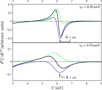
Figure 9: Elastic (blue dashed), inelastic (green dashed) contribution to the total (black solid) second derivative of the current $d^{2}I/dU^{2}$ in the superconducting state for different peak width $\gamma_{0}$. The additional inelastic contribution will lead to a peak-dip feature with similar positive and negative amplitude in the second derivative, whereas the purely elastic contribution only pronounces the dip at the shifted phonon frequency $eU\approx\Delta+\omega_{0}$ strongly.

The value $A_{0}$ is choosen such that the dimensionless electron-phonon coupling constant $\lambda=2\int_{0}^{\infty}d\omega\,\alpha^{2}F(\omega)/\omega=1.5$. We use $\mu^{*}=0.1$ for the pseudopotential, such that solving the Eliashberg equations yields a gap value $\Delta\simeq 1\text{ meV}$. In Fig. 9 we see the resulting second derivative of the tunneling current, which is more sensitive to the fine-structure than the conductance, for the above mentioned elastic and inelastic tunneling for different peak width $\gamma_{0}$ in the superconducting state. As was seen in the experiments we use the ratio $\left|t^{\text{i}}/t^{\text{e}}\right|^{2}\approx 0.12/\int_{0}^{10\text{ meV}}d\omega\,\alpha^{2}F(\omega)$. The inelastic contribution Eq. (22) has its major contribution for frequencies a bit below the energy of the phonon peaks shifted by the gap $\Delta$. Since inelastic tunneling adds additional channels to the conductance, its contribution will have the opposite sign of the elastic contribution in (16) and can give pronounced positive peaks in the second derivative of the tunneling current followed by a negative peak of same amplitude . These symmetric peak-dip features around the zero axis in the second derivative of the tunneling current are characteristic for the joint elastic and inelastic STM. In the present example, we were not able to find an Eliashberg function that would yield such a tunneling spectra from the purely elastic tunneling contribution Eq. (16). Even for very sharp Eliashberg spectra where the second derivative of the tunneling current can be clearly positive for some voltages, see upper picture in Fig. 9, the following dip will always be much more pronounced if one only considers the elastic tunneling contribution.

Appendix C Modelling of experimental broadening

The experimental resolution is limited due to the used lock-in technique. As was shown in Ref. Klein73, , for a modulation voltage $V_{\text{mod}}$ (the modulation voltages stated in this work are root mean square values $U_{\text{mod}}=U_{\text{mod,max}}/\sqrt{2}$) the experimental curve for the second derivative measurements is the actual current convoluted with a Gaussian function $\Gamma(\omega)$ of half-width FWHM$\approx 1.7eV_{\text{mod}}$. This corresponds in our case to a standard deviation $\sigma=\text{FWHM}/2.4=0.31\text{meV}$. For the elastic part this means that we get

$$\frac{d^{2}I^{\text{e,exp}}}{dU^{2}} =-\sigma_{0}\int_{-\infty}^{\infty}dEd\omega\,\Gamma(eU-E)n_{F}^{\prime}(\omega+E)\tilde{\nu}_{S}(\omega)$$ (26)

which can be easily computed using the fermionic DOS obtained from solving the Eliashberg equations.

Let us now consider the experimental broadening for inelastic tunneling and restrict us to the case of positive bias voltages. Following Eq. (25), the second derivative of the inelastic tunneling current is for positive $U>0$ given by

$$\frac{d^{2}I^{\text{i}}}{dU^{2}} =e\sigma_{0}\left|\frac{t^{\text{i}}}{t^{\text{e}}}\right|^{2}\int_{-\infty}^{\infty}d\omega\,\alpha^{2}F_{\text{tun}}^{T}{}^{\prime}(eU+\omega)\tilde{\nu}_{S}(\omega)n_{F}(\omega)$$ (27)

To get the experimental data (both in the normal and superconducting state), we have to broaden the function by the convolution

$$\frac{d^{2}I^{\text{i,exp}}}{dU^{2}} =e\sigma_{0}\left|\frac{t^{\text{i}}}{t^{\text{e}}}\right|^{2}\int_{-\infty}^{\infty}dE\,\Gamma(eU-E)$$ (28)

$$\hskip 36.98866pt\int_{-\infty}^{\infty}d\omega\,\alpha^{2}F_{\text{tun}}^{T}{}^{\prime}(E+\omega)\tilde{\nu}_{S}(\omega)n_{F}(\omega)$$

$$=e\sigma_{0}\left|\frac{t^{\text{i}}}{t^{\text{e}}}\right|^{2}\int d\omega\,\alpha^{2}F_{\text{tun}}^{\text{exp}}{}^{\prime}(eU+\omega)\tilde{\nu}_{S}(\omega)n_{F}(\omega)$$

with the thermally and modulation voltage broadened spectral function

$$\alpha^{2}F_{\text{tun}}^{\text{exp}}(x)=\int_{-\infty}^{\infty}dy\Gamma(x-y)\alpha^{2}F_{\text{tun}}^{T}(y)$$ (29)

In the normal state $\tilde{\nu}_{S}(\omega)\approx 1$ this simplifies in the limit of small temperatures $T\ll\omega_{D},E_{F}$ (such that $n_{F}(\omega)\approx\theta(-\omega)$) to

$$\frac{d^{2}I_{\text{nc}}^{\text{i,exp}}}{dU^{2}} \approx e\sigma_{0}\left|\frac{t^{\text{i}}}{t^{\text{e}}}\right|^{2}\int_{-\infty}^{\infty}d\omega\,\alpha^{2}F_{\text{tun}}^{\text{exp}}{}^{\prime}(eU+\omega)n_{F}(\omega)$$

$$=e\sigma_{0}\left|\frac{t^{\text{i}}}{t^{\text{e}}}\right|^{2}\alpha^{2}F_{\text{tun}}^{\text{exp}}(eU)$$ (30)

As $\frac{d^{2}I_{\text{nc}}^{\text{e,exp}}}{dU^{2}}\approx 0$, we can extract the $\alpha^{2}F_{\text{tun}}^{T,\text{mod}}(eU)$ function from the normal state measurements and can then use it to calculate the inelastic current in the superconducting state.

Appendix D Multiple phonon processes

If we consider tunneling processes with a higher number of excited phonons we can formally write down the following tunneling processes

$$\delta H_{\text{t}}^{(n)} =\frac{1}{\sqrt{V_{t}}V_{S}^{\frac{n+1}{2}}}\sum_{\textbf{{k}},\textbf{{p}},\textbf{{q}}_{1},\ldots,\textbf{{q}}_{n}\atop\sigma,\mu_{1},\ldots,\mu_{n}}T_{\textbf{{k}},\textbf{{p}},\textbf{{q}}_{1},\ldots,\textbf{{q}}_{n},\mu_{1},\ldots,\mu_{n}}^{\text{i}}$$

$$\quad\alpha_{\textbf{{q}}_{1},\mu_{1}}\ldots\alpha_{\textbf{{q}}_{n},\mu_{n}}c_{\textbf{{k}},\sigma}^{\dagger}c_{\textbf{{p}},\sigma}\phi_{\textbf{{q}}_{1},\mu_{1}}\ldots\phi_{\textbf{{q}}_{n},\mu_{n}}$$ (31)

In the zero temperature limit it is then straightforward to generalize the result (21) to the n-phonon process (demanding energy conservation and Fermi statistic for the leads)

$$I^{\text{i},(n)} =4\pi e\nu_{T}^{0}\left|t^{\text{i},(n)}\right|^{2}\int d\omega_{1}\ldots d\omega_{n}d\omega_{n+1}\alpha^{2}F_{\text{tun}}(\omega_{1})\ldots\alpha^{2}F_{\text{tun}}(\omega_{n})\nu_{S}(\omega_{n+1})$$ (32)

$$\hskip 5.69054pt\biggl{[}\theta(-\omega_{n+1})\theta(\omega_{n+1}-\omega_{n}-\ldots-\omega_{1}+eU)-\{\omega_{n+1},U\rightarrow-\omega_{n+1},-U\}\biggr{]}$$

For the conductance, we then find for particle-hole symmetric systems

$$\frac{dI^{\text{i},(n)}}{dU} =\sigma_{0}\left|\frac{t^{\text{i},(n)}}{t^{\text{e}}}\right|^{2}\text{sign}(U)\int_{0}^{\infty}d\omega d\omega_{1}\ldots d\omega_{n-1}\alpha^{2}F_{\text{tun}}(e\left|U\right|-\omega-\omega_{1})\alpha^{2}F_{\text{tun}}(\omega_{1}-\omega_{2})\ldots\alpha^{2}F_{\text{tun}}(\omega_{n-2}-\omega_{n-1})\tilde{\nu}_{S}(\omega)$$

$$=\sigma_{0}\left|\frac{t^{\text{i},(n)}}{t^{\text{e}}}\right|^{2}\text{sign}(U)\int_{0}^{\infty}d\omega\,\alpha^{2n}F_{\text{tun}}^{n}(e\left|U\right|-\omega)\tilde{\nu}_{S}(\omega)$$ (33)

where we defined the convolution

$$\alpha^{2n}F_{\text{tun}}^{n}(\omega) =\int_{0}^{\infty}d\omega_{1}\ldots d\omega_{n-1}\,\alpha^{2}F_{\text{tun}}(\omega-\omega_{1})\alpha^{2}F_{\text{tun}}(\omega_{1}-\omega_{2})\ldots\alpha^{2}F_{\text{tun}}(\omega_{n-2}-\omega_{n-1})$$ (34)

Appendix E Important relations of Non-Equilibrium propagators

Following Ref. [Keldyshbook, ] we define for both the fermionic and the bosonic fields $\phi(t)$ the greater, lesser, time-ordered and anti-time-ordered Green’s functions as

$$\begin{split}G^{<}(t,t^{\prime})&=G^{+-}(t,t^{\prime})=-i\langle\,{\phi^{+}(t)\bar{\phi}^{-}(t^{\prime})}\,\rangle\\ G^{>}(t,t^{\prime})&=G^{-+}(t,t^{\prime})=-i\langle\,{\phi^{-}(t)\bar{\phi}^{+}(t^{\prime})}\,\rangle\\ G^{\mathcal{T}}(t,t^{\prime})&=G^{++}(t,t^{\prime})=-i\langle\,{\phi^{+}(t)\bar{\phi}^{+}(t^{\prime})}\,\rangle\\ G^{\tilde{\mathcal{T}}}(t,t^{\prime})&=G^{--}(t,t^{\prime})=-i\langle\,{\phi^{-}(t)\bar{\phi}^{-}(t^{\prime})}\,\rangle\end{split}$$ (35)

We can now perform the Keldysh rotation to the classical and quantum fields in the bosonic case:

$$\begin{split}\phi^{\text{cl}}(t)&=\frac{1}{\sqrt{2}}\bigl{[}\phi^{+}(t)+\phi^{-}(t)\bigr{]}\\ \phi^{\text{q}}(t)&=\frac{1}{\sqrt{2}}\bigl{[}\phi^{+}(t)-\phi^{-}(t)\bigr{]}\end{split}$$ (36)

and similar for the conjugate fields $\bar{\phi}(t)$. However, for the fermionic fields we use the Ovchinnikov-Larkin convention [Larkin, ]

$$\begin{split}\phi^{\text{1}}(t)&=\frac{1}{\sqrt{2}}\bigl{[}\phi^{+}(t)+\phi^{-}(t)\bigr{]}\\ \phi^{\text{2}}(t)&=\frac{1}{\sqrt{2}}\bigl{[}\phi^{+}(t)-\phi^{-}(t)\bigr{]}\\ \bar{\phi}^{\text{1}}(t)&=\frac{1}{\sqrt{2}}\bigl{[}\bar{\phi}^{+}(t)-\bar{\phi}^{-}(t)\bigr{]}\\ \bar{\phi}^{\text{2}}(t)&=\frac{1}{\sqrt{2}}\bigl{[}\bar{\phi}^{+}(t)+\bar{\phi}^{-}(t)\bigr{]}\end{split}$$ (37)

For the fermionic and bosonic cases, the retarded, advanced and Keldysh propagators are then defined as in Eq. (7). The relations between the different Green’s functions ($>,<,\mathcal{T},\tilde{\mathcal{T}},R,A,K$) can be summarized by

$$\begin{split}0&=G^{\mathcal{T}}+G^{\tilde{\mathcal{T}}}-G^{>}-G^{<}\\ G^{K}&=G^{>}+G^{<}\\ G^{R}&=\frac{1}{2}\bigl{[}G^{\mathcal{T}}-G^{\tilde{\mathcal{T}}}+G^{>}-G^{<}\bigr{]}\\ G^{A}&=\frac{1}{2}\bigl{[}G^{\mathcal{T}}-G^{\tilde{\mathcal{T}}}-G^{>}+G^{<}\bigr{]}\end{split}$$ (38)

References

• (1) J. Bardeen, L. N. Cooper, and J. R. Schrieffer, Phys. Rev. 108, 1175 (1957).
• (2) I. Giaever, Phys. Rev. Lett. 5, 147 (1960).
• (3) J. Nicol, S. Shapiro, and P. H. Smith, Phys. Rev. Lett. 5, 461 (1960).
• (4) G. M. Eliashberg, Sov. Phys. JETP 11, 696 (1960).
• (5) I. Giaever, H. R. Hart, and K. Mergele, Phys. Rev. 126, 941 (1962).
• (6) J. R. Schrieffer, D. J. Scalapino, and J. W. Wilkins, Phys. Rev. Lett. 10, 336 (1963).
• (7) J. M. Rowell, A. G. Chynoweth, and J. C. Phillips, Phys. Rev. Lett. 9, 59 (1962).
• (8) J. M. Rowell, P.W. Anderson, and D.E. Thomas, Phys. Rev. Lett. 10, 334 (1963).
• (9) W. McMillan and J. Rowell, Superconductivity Vol. 1, ed. R. D. Parks (Dekker, New York, 1969) pp. 561-611.
• (10) I. Giaever, Science 183, 1253 (1974).
• (11) W. L. McMillan and J. M. Rowell, Phys. Rev. Lett. 14, 108 (1965).
• (12) D.J. Scalapino, J. W. Wilins, Phys. Rev. 148, 263-279 (1966).
• (13) J.P. Carbotte, Rev. Mod. Phys. 62, 1027 (1990).
• (14) A. Leger and J. Klein, Phys. Lett. 28A, 751 (1969)..
• (15) J. M. Rowell, W. L. McMillan, and W. Feldmann, Phys. Rev. 180, 658 (1969).
• (16) W. Wattamanuik, H. Kreuzer, and J. Adler, Physics Letters A 37, 7 (1971).
• (17) J. Klein, A. Léger, M. Belin, D. Défourneau, and M. J. L. Sangster, Phys. Rev. B 7, 2336 (1973).
• (18) M.E. Taylor, Ultramicroscopy 42, 215 (1992).
• (19) M. Schackert, T. Märkl, J. Jandke, M. Holzer, S. Ostanin, E. K. U. Gross, A. Ernst, W. Wulfhekel, Phys. Rev. Lett. 114, 047002 (2015).
• (20) Alan J. Bennett, C. B. Duke and S. D. Silverstein, Phys. Rev. 176, 969 (1968).
• (21) C. Berthod, T. Giamarchi, Phys. Rev. B 84, 155414 (2011).
• (22) J. Bardeen, Phys. Rev. Lett. 6, 57 (1961).
• (23) M. H. Cohen, L. M. Falicov, and J. C. Phillips, Phys. Rev. Lett. 8, 316 (1962).
• (24) Gerald D. Mahan , Many-Particle Physics, Springer, 3rd ed. (2000) .
• (25) J. R. Kirtley and D. J. Scalapino, Phys. Rev. Lett. 65, 798 (1990).
• (26) Ming-wen Xiao, Zheng-zhong Li, Physica C: Superconductivity 221, 136 (1994).
• (27) A. V. Gold, Philos. Mag. 5, 70 (1960).
• (28) L. Zhang, T. Miyamachi, T. Tomanić, R. Dehm, and W. Wulfhekel, Rev. Sci. Instr. 82, 103702 (2011).
• (29) W. McMillan , Phys. Rev. 167, 331 (1968).
• (30) Brun, C. and Hong, I-Po and Patthey, F. and Sklyadneva, I. Yu. and Heid, R. and Echenique, P. M. and Bohnen, K. P. and Chulkov, E. V. and Schneider, Wolf-Dieter, Phys. Rev. Lett. 102, 207002, (2009).
• (31) D. Eom, S. Qin, M.-Y. Chou, and C. K. Shih, Phys. Rev. Lett. 96, 027005 (2006).
• (32) I. B. Altfeder, K. A. Matveev, and D. M. Chen, Phys. Rev. 78, 2815 (1997).
• (33) H. H. Weitering, D. R. Heslinga, and T. Hibma, Phys. Rev. B 45, 5991 (1992).
• (34) M. Jalochowski, H. Knoppe, G. Lilienkamp and E. Bauer, Phys. Rev. B 46, 4693 (1992).
• (35) I. Yu. Sklyadneva, R. Heid, K.-P. Bohnen, P. M. Echenique and E.V. Chulkov, Phys. Rev. B 87, 085440 (2013) .
• (36) R. Heid, K.-P. Bohnen, I. Yu. Sklyadneva, and E. V. Chulkov, Phys. Rev. B 81, 174527 (2010).
• (37) B. N. Brockhouse, T. Arase, G. Caglioti, K. R. Rao, and A. D. B. Woods, Phys. Rev. 128, 1099 (1962).
• (38) Charles Kittel, “Introduction to solid state physics”, Wiley New York (2005).
• (39) T. Nishio, M. Ono, T. Eguchi, H. Sakata, and Y. Hasegawa, Appl. Phys. Lett. 88, 113115 (2006).
• (40) T. Nishio, T. An, A. Nomura, K. Miyachi, T. Eguchi, H. Sakata, S. Lin, N. Hayashi, N. Nakai, M. Machida, and Y. Hasegawa, Phys. Rev. Lett. 101, 167001 (2008).
• (41) S. Qin, J. Kim, Q. Niu, C-K. Shin, Science 324, 1314 (2009).
• (42) A. M. Garcia-Garcia, J. D. Urbina, K. Richter, E. A. Yuzbashyan, B. L. Altshuler, Phys. Rev. B 83, 014510 (2011)
• (43) S. Bose, A. M. García-García, M. M. Ugeda, J. D. Urbina. C. H. Michaelis, I. Brihuega and K. Kern, Nat. Mat. 9, 550 (2010)
• (44) A.A. Galkin, A.I. D’yachenko, V.M. Svistunov, JETP, Vol. 39, No. 6, p. 1115 (1974)
• (45) J. Schmalian, M. Langer, S. Grabowski and K. H. Bennemann, Computer Physics Communications 93, 141 (1996).
• (46) J. Rossat-Mignod, L. Regnault, C. Vettier, P. Bourges, P. Burlet, J. Bossy, J. Henry, and G. Lapertot, Physica C 86, 185 (1991).
• (47) H. A. Mook, M. Yethiraj, G. Aeppli, T. E. Mason, and T. Armstrong, Phys. Rev. Lett. 70, 3490 (1993).
• (48) H. Fong, P. Bourges, Y. Sidis, L. Regnault, A. Ivanov, G. Gu, N. Koshizuka, and B. Keimer, Nature 398, 588 (1999).
• (49) A. D. Christianson, E. A. Goremychkin, R. Osborn, S. Rosenkranz, M. D. Lumsden, C. D. Malliakas, I. S. Todorov, H. Claus, D. Y. Chung, M. G. Kanatzidis, R. I. Bewley, and T. Guidi, Nature 456, 930 (2008).
• (50) D.S. Inosov, P. B.J.T. Park, D.L. Sun, Y. Sidis, A. Schneidewind, K. Hradil, D. Haug, C.T. Lin, B. Keimer, and V. Hinkov, Nat. Phys. 6, 178 (2010).
• (51) A. Abanov, A. Chubukov and J. Schmalian, J. Electron Spectrosc. Relat. Phenom. 117, 129 (2001).
• (52) H. Suderow, E. Bascones, A. Izquierdo, F. Guinea, S. Vieira, Phys. Rev. B 65, 100519(R) 2002.
• (53) A. Kamenev, Field theory of non-equilibrium systems, Cambridge Univ. Press (2011)
• (54) A. I. Larkin and Y. N. Ovchinnikov, Sov. Phys. JETP 41, 960 (1975)