Edge of chaos as critical local symmetry breaking in dissipative nonautonomous systems

Abstract

The fully nonlinear notion of resonance$-$geometrical resonance$-$in the general context of dissipative systems subjected to spatially periodic phase-modulated potentials is discussed. It is demonstrated that there is an exact local invariant associated with each geometrical resonance solution which reduces to the system’s energy when the potential is stationary. The geometrical resonance solutions represent a local symmetry whose critical breaking leads to a new analytical criterion for the onset of chaotic instabilities. This physical criterion is deduced in the co-moving frame from the local energy conservation over the shortest significant timescale. Remarkably, the new physical criterion for the onset of chaotic instabilities is shown to be valid over large regions of parameter space, thus being useful beyond the scope of current mathematical techniques. More importantly, the present theory helps to understand the unreasonable effectiveness of the Melnikov’s method beyond the perturbative regime.

I
INTRODUCTION

Hamiltonian and dissipative systems have traditionally been studied separately due to their clearly different dynamic properties [1]: dissipation forces give rise to the existence of transient dynamics associated with the basins of the different attractors, while the Poincaré integral invariants of Hamiltonian systems lead to special behaviour of the eigenvalues of equilibria and periodic orbits, and to existence theorems for various types of orbits such as the celebrated Kolmogorov-Arnold-Moser theorem. To date, only the notion of geometrical resonance (GR) [2] has been able to provide a deep link between autonomous Hamiltonian and non-autonomous dissipative systems in the sense that it offers a universal procedure with which to locally ”Hamiltonianize” an otherwise dissipative system by suitably choosing the non-autonomous term(s) $f_{i}(t)$ such that the system’s energy is conserved locally: $f_{i}(t)=f_{i,GR}(t)$. The original formulation of GR analysis was for standing potentials [2], and was applied to diverse nonlinear problems involving such potentials [3-11], including the stability of the responses of an overdamped bistable system [7], the suppression of spatio-temporal chaos and the stabilization of localized solutions in general spatio-temporal systems [5,8-10], quantum control in trapped Bose-Einstein condensates (BECs) [11], and the characterization of periodic solutions of a fractional Duffing’s equation [12].

On the other hand, a major body of research has considered modulated potentials appearing in different physical contexts such as synchrotron motion of beams [13], BECs in optical lattices [14], Shapiro steps and chaos in Frenkel-Kontorova chains [15], and nanoscale devices powered by the lateral Casimir force [16], just to cite a few representative examples. In general, the reference frames co-moving with modulated potentials are accelerating frames, which introduces an additional complexity into analysis of the dynamics relative to the laboratory reference frame (L-frame). Since GR is neither more nor less than a local symmetry, namely that the dynamics equations remain locally invariant under time reversal when the non-autonomous terms are suitably locally chosen, $f_{i}(t)=f_{i,GR}(t)$, it seems appropriate and pertinent to explore its implications in general systems.

The article is structured as follows. In Sec. II, new properties of this subtle symmetry in the generalized context of dissipative systems in phase-modulated potentials are characterized and exploited to determine a physical criterion for the onset of chaotic instabilities in parameter space whose accuracy and scope goes beyond current perturbative mathematical techniques. The theory is discussed through the paradigmatic model of a particle subjected to a spatially periodic and temporally shaken potential which describes, for example, the chaotic phase oscillation of a proton beam in a cooler synchrotron [13]. Section III includes a summary of the main results and conclusions. Some details of the analytical calculations are relegated to the Appendices.

II GEOMETRICAL RESONANCE ANALYSIS

II.1 Theory

Let us consider the class of non-autonomous dissipative systems

$$\overset{..}{x}=g\left(x,t\right)-d\left(x,\overset{.}{x}\right),$$ (1)

where the overdot denotes $d/dt$, $g\left(x,t\right)\equiv-\partial V\left(x,t\right)/\partial x$, with $V\left(x,t\right)\equiv V\left[x-f(t)\right]$ being a modulated and spatially periodic potential while $f\left(t\right)$ is an a priori arbitrary (twice-differentiable) function of time, and where $-d\left(x,\overset{.}{x}\right)$ is a generic dissipative force. In the potential reference frame (V-frame) with $z\left(t\right)=x\left(t\right)-f(t)$, Eq. (1) reads

$$\overset{..}{z}=g\left(z\right)-d\left(z,\overset{.}{z},f,\overset{.}{f},t\right)-\overset{..}{f}.$$ (2)

In general, if $z_{GR}(t)$ is a GR solution of Eq. (2), it must satisfy

$$\overset{..}{z}_{GR} =g\left(z_{GR}\right),$$ (3)

$$\overset{..}{f}_{GR} =-d\left(z_{GR},\overset{.}{z}_{GR},f_{GR},\overset{.}{f}_{GR},t\right),$$ (4)

and hence

$$x_{GR}\equiv z_{GR}+f_{GR}$$ (5)

is a GR solution of Eq. (1) for a given set of initial conditions $\left[x_{0}\equiv x(t=0),\overset{.}{x}_{0}\equiv\overset{.}{x}\left(t=0\right)\right]$. After assuming that $V(z)$ is infinitely differentiable, definitions (3)-(5) give rise to the following distinguishing properties. First, in contrast with the case of standing potentials [2], where $f_{GR}$ is univocally determined from an algebraic equation involving the single GR solution associated with a given set of initial conditions, one has to solve a differential equation for $f_{GR}$ in the present general case and obtain the initial values $f_{GR}\left(t=0\right)\equiv f_{GR,0},\overset{.}{f}_{GR}(t=0)\equiv\overset{.}{f}_{GR,0}$ as a part of the whole solution. This is because the GR scenario for modulated potentials involves two reference frames, the V-frame being non-inertial in the general case. Second, conditions (3)-(4) are equivalent to the local (i.e., dependent on the initial conditions) energy conservation requirement

$$(1/2)\overset{.}{z}_{GR}^{2}+V\left[z_{GR}\right]\equiv E_{GR}=const$$ (6)

in the V-frame, while one has the requirement of a different local invariant in the L-frame:

$$I_{GR}\equiv\frac{\overset{.}{x}_{GR}^{2}}{2}+V\left[x_{GR}-f_{GR}\right]+\overset{.}{f}_{GR}\left(\frac{\overset{.}{f}_{GR}}{2}-\overset{.}{x}_{GR}\right)=const.$$ (7)

After Taylor expanding the potential, the local invariant $I_{GR}$ can be recast into the more transparent form

$$(1/2)\overset{.}{x}_{GR}^{2}+V\left[x_{GR}-f_{GR,0}\right]+S_{GR}=const,$$ (8)

where,

$$S_{GR} \equiv\sum_{n=1}^{\infty}\frac{\left(-1\right)^{n}}{n!}(f_{GR}^{\ }-f_{GR,0})^{n}V^{\left(n\right)}\left[x_{GR}-f_{GR,0}\right]$$

$$+\overset{.}{f}_{GR}\left(\overset{.}{f}_{GR}/2-\overset{.}{x}_{GR}\right),$$ (9)

with $V^{\left(n\right)}\equiv d^{n}V(z)/dz^{n}$. From Eq. (8) one sees that, under GR conditions, the energy associated with the corresponding standing potential is not (locally) conserved in the L-frame, as expected, while the new invariant $I_{GR}$ allows the temporal evolution of this energy to be calculated for each GR solution. Third, in the Hamiltonian limiting case, i.e., $d\left(x,\overset{.}{x}\right)\rightarrow 0$, Eq. (4) becomes $\overset{..}{f}_{GR}=0$, and hence $f_{GR}(t)=Vt$ with $V$ being an arbitrary constant and where an additional additive constant has been taken to be zero without loss of generality. This means that, in the absence of dissipation, GR solutions are solely possible for potentials traveling with constant speed, i.e., for inertial frames, as expected. And fourth, a GR solution will be observed if it is stable, i.e., if any small perturbation $\delta z\left(t\right)$ of $z_{GR}\left(t\right)$ is damped. After substituting $z(t)=z_{GR}\left(t\right)+\delta z\left(t\right)$ into Eq. (2) with $f\left(t\right)=f_{GR}\left(t\right)$, one obtains the linearized equation of motion for small perturbations $\delta z\left(t\right)$:

$$\overset{..}{\delta z}+\left(\frac{\partial d}{\partial\overset{.}{z}}\right)_{GR}\overset{.}{\delta z}+\left[\left(\frac{\partial d}{\partial z}\right)_{GR}-\left(\frac{dg}{dz}\right)_{GR}\right]\delta z=0.$$ (10)

Note that this generalized Hill equation with dissipation also governs the stability of the GR solutions in the L-frame (cf. Eq. (5)). It is shown below that this stability analysis together with the dependence of the GR solutions on the system’s parameters and the local invariants (6) and (8) allows one to get a new analytical criterion for the order-chaos threshold from the weakest useful approximation to the local energy conservation in the V-frame.

II.2 Paradigmatic model

To demonstrate the effectiveness of the present GR theory in a simple paradigmatic model, consider the dissipative dynamics of a particle subjected to a spatially periodic and temporally shaken potential:

$$\overset{..}{x}+\sin\left[x-f(t)\right]=-\eta\overset{.}{x}.$$ (11)

The dimensionless Eq. (11) describes for example the pinion motion of a nanoscale device composed of a pinion and a rack coupled via the lateral Casimir force, where $\eta>0$ is a damping coefficient while $f(t)$ accounts for the a priori arbitrary horizontal motion of the rack [16]. In the V-frame with $z\left(t\right)=x\left(t\right)-f(t)$, Eq. (11) reads

$$\overset{..}{z}+\sin z=-\eta\overset{.}{z}-\eta\overset{.}{f}-\overset{..}{f}.$$ (12)

Thus, GR solutions of Eq. (12) must satisfy

$$\overset{..}{z}_{GR}+\sin z_{GR} =0,$$ (13)

$$\overset{.}{z}_{GR}+\overset{.}{f}_{GR}+\overset{..}{f}_{GR}/\eta =0.$$ (14)

Exact analytical periodic solutions of the integrable pendulum (13) [17] corresponding to libration and rotation motions are given by

$$z_{GR}^{l}(t;t_{0},m) =2\arcsin\left[\sqrt{m}\operatorname*{sn}\left(t-t_{0};m\right)\right],$$

$$\overset{.}{z}_{GR}^{l}(t;t_{0},m) =2\sqrt{m}\operatorname{cn}\left(t-t_{0};m\right),$$ (15)

and

$$z_{GR}^{r}(t;t_{0},m) =\pm 2\operatorname{am}\left[\left(t-t_{0}\right)/\sqrt{m};m\right],$$

$$\overset{.}{z}_{GR}^{r}(t;t_{0},m) =\pm\frac{2}{\sqrt{m}}\operatorname*{dn}\left[\frac{t-t_{0}}{\sqrt{m}};m\right],$$ (16)

respectively, where $\operatorname*{sn}\left(\cdot;m\right)$, $\operatorname{cn}\left(\cdot;m\right)$, $\operatorname*{dn}\left(\cdot;m\right)$, $\operatorname{am}\left(\cdot;m\right)$ are Jacobian elliptic functions of parameter $m\in\left]0,1\right[$, the upper (lower) sign in the rotation solutions refers to counterclockwise (clockwise) rotations, while $t_{0}$ is an arbitrary initial time. These solutions have the respective periods $T^{l}\left(m\right)\equiv 4K$ and $T^{r}(m)\equiv 2\sqrt{m}K$, where $K\equiv K(m)$ is the complete elliptic integral of the first kind [18]. Although the parameters corresponding to libration and rotation motions are inversely related each other, the same notation, $m$, is used here since both parameters are defined over the same interval [17] and there is no possibility of confusion in the subsequent analysis. Also, definition $\operatorname*{sn}\left(\cdot;m\right)\equiv\sin\left[\operatorname{am}\left(\cdot;m\right)\right]$ has been used to write a simpler alternative expression for $z_{GR}^{r}(t;t_{0},m)$. After taking $t_{0}=0$ for simplicity, using the Fourier series of the Jacobian elliptic functions involved [18], and integrating the linear differential equation (14), one straightforwardly obtains the GR excitations

$$f_{GR}^{l}(t) \equiv C_{1}+C_{2}\operatorname{e}^{-\eta t}+\sum_{n=0}^{\infty}b_{n}\cos\left(\omega_{n}t+\varphi_{n}\right),$$

$$f_{GR}^{r}(t) \equiv C_{1}^{\prime}+C_{2}^{\prime}\operatorname{e}^{-\eta t}\mp\frac{\pi t}{\sqrt{m}K}\pm\sum_{n=1}^{\infty}b_{n}^{\prime}\cos\left(\omega_{n}^{\prime}t+\varphi_{n}^{\prime}\right),$$ (17)

and the corresponding GR solutions in the L-frame

$$x_{GR}^{l}(t) =C_{1}+C_{2}\operatorname{e}^{-\eta t}+\sum_{n=0}^{\infty}\frac{b_{n}}{\operatorname*{tg}\varphi_{n}}\sin\left(\omega_{n}t+\varphi_{n}\right),$$

$$x_{GR}^{r}(t) =C_{1}^{\prime}+C_{2}^{\prime}\operatorname{e}^{-\eta t}\pm\sum_{n=1}^{\infty}\frac{b_{n}^{\prime}}{\operatorname*{tg}\varphi_{n}^{\prime}}\sin\left(\omega_{n}^{\prime}t+\varphi_{n}^{\prime}\right),$$ (18)

with

$$b_{n} \equiv\frac{2\pi\eta}{\omega_{n}K\sqrt{\eta^{2}+\omega_{n}^{2}}}\operatorname{sech}\left[\frac{\left(2n+1\right)\pi K^{\prime}}{2K}\right],$$

$$b_{n}^{\prime} \equiv\frac{2\pi\eta}{\omega_{n}^{\prime}K\sqrt{m}\sqrt{\eta^{2}+\omega_{n}^{\prime 2}}}\operatorname{sech}\left(\frac{n\pi K^{\prime}}{K}\right),$$

$$\omega_{n} \equiv\left(n+1/2\right)\pi/K,$$

$$\omega_{n}^{\prime} \equiv n\pi/\left(\sqrt{m}K\right),$$

$$\varphi_{n} \equiv\arctan\left(\eta/\omega_{n}\right),$$

$$\varphi_{n}^{\prime} \equiv\arctan\left(\eta/\omega_{n}^{\prime}\right)$$ (19)

and where $C_{1,2},C_{1,2}^{\prime}$ are constants to be determined from the initial conditions $\left(x_{0},\overset{.}{x}_{0}\right)$ (see Appendix A), $K^{\prime}\equiv K(1-m)$, while the upper (lower) sign in Eqs. (17) and (18) refers to counterclockwise (clockwise) rotations. These GR solutions have the following properties. (i) Their stability is governed by Eq. (10), i.e.,

$$\overset{..}{\delta z}+\eta\overset{.}{\delta z}+\cos z_{GR}^{l,r}\delta z=0,$$ (20)

which reduces to the Lamé equations

$$\frac{d^{2}u}{dt^{2}}+\left[1-\eta^{2}/4-2m\operatorname{sn}^{2}\left(t;m\right)\right]u =0,$$ (21)

$$\frac{d^{2}v}{d\tau^{2}}+\left[m\left(1-\eta^{2}/4\right)-2m\operatorname{sn}^{2}\left(\tau;m\right)\right]v =0,$$ (22)

where $u=\exp\left(\eta t/2\right)\delta z$ and $v=\exp\left(\eta\sqrt{m}\tau/2\right)\delta z$ for librations and rotations, respectively. Standard results for these Lamé equations [19,20] indicate that Eq. (20) presents only one instability region in the $m-\eta$ parameter plane. A careful comparison of Eq. (21) with Eq. (22) leads one to expect the instability region for librations to be clearly narrower than that for rotations owing to the term $m\left(1-\eta^{2}/4\right)<1-\eta^{2}/4$ since $m\in\left]0,1\right[$. Moreover, the maximum range of $\eta$ values in the instability regions is expected to occur when $m\simeq 1$ for both kinds of motion due to all GR solutions $z_{GR}^{l,r}\left(t\right)$ converging to the separatrix (the most unstable phase path) of the integrable pendulum as $m\rightarrow 1$. Numerical simulations confirmed these expectations, as is shown in Fig. 1. (ii) For any set of initial conditions not on the unperturbed separatrix, i.e., for any GR excitation (17) and corresponding solution (18), one sees that the dependence of each harmonic of such excitations and solutions on the damping coefficient has exactly the same form: $\eta/\sqrt{\eta^{2}+\alpha}$, with $\alpha$ being a function of the corresponding natural period. From this it can be inferred that, for a periodic excitation $f(t)$ of amplitude $\gamma$, the dependence of the chaotic-threshold amplitude, $\gamma_{th}$, on $\eta$ should obey this functional form irrespective of the value of $\eta$, an unanticipated result in view of the perturbative character of the current mathematical techniques to predict the onset of chaos (Melnikov’s method (MM) [21]). (iii) Since harmonic functions are commonly used to model periodic excitations, the GR solution corresponding to libration near the bottom of the potential well (i.e., $x_{0},\approx 0,\overset{.}{x}_{0}\approx 0,m\gtrsim 0$) is of especial interest. One straightforwardly obtains the steady $(t\gg\eta^{-1})$ solutions (cf. Eqs. (17) and (18))

$$x_{GR}^{l}(t) =2\sqrt{m}\sin t+f_{GR}^{l}(t),$$

$$f_{GR}^{l}(t) =\frac{2\sqrt{m}\eta}{\sqrt{1+\eta^{2}}}\cos\left(t+\arctan\eta\right)+O\left(m^{3/2}\right),$$ (23)

while the corresponding local invariant (8) reduces to

$$I_{GR}^{l} =(1/2)\overset{.}{x}_{GR}^{l2}\left(t\right)-\cos x_{GR}^{l}\left(t\right)+\frac{f_{GR}^{l2}(t)+\overset{.}{f}_{GR}^{l2}(t)}{2}$$

$$+O\left(m^{3}\right),$$ (24)

i.e., $I_{GR}^{l}\left(t\right)$ is no more than the sum of the energy associated with the limiting case of standing potential plus the energy associated with the V-frame moving as a linear harmonic oscillator of period $2\pi$, which is an unexpected result. (iv) In the Hamiltonian limiting case, i.e., $\eta\rightarrow 0$, GR solutions for librations are not possible due to their oscillatory character around a fixed point is incompatible with the requirement of a traveling potential function (cf. third property in the previous subsection), while GR solutions for rotations are indeed possible (see Eq. (17)). (v) In the limit of very high dissipation $\left(\eta\rightarrow\infty\right)$, the steady GR solutions are equilibria (cf. Eqs. (18) and (23)), as expected.

Figure 1: Stability-instability charts obtained by numerical integration of the Lamé’s equations (a) Eq. (21) and (b) Eq. (22) for libration and rotation motions, respectively, where instability regions are indicated by dots. The insets show the tips of the instability tongues when $m\rightarrow 1$ and $\eta\rightarrow 0$.

II.3 Order-chaos threshold

Next, one can use the above properties of the GR solutions to obtain an analytical estimate of the order-chaos threshold associated with a generic $T$-periodic excitation $f_{g}(t)$ of amplitude $\gamma$. In general this generic excitation will not exactly correspond to any GR excitation function (17), and hence one cannot expect strict conservation (i.e., over an infinite timescale) of the invariants (6) and (7) for any set of initial conditions. Indeed, the energy rate is governed in the V-frame by the equation (cf. Eq. (12))

$$\frac{dE}{dt}=-\eta\overset{.}{z}^{2}-\eta\overset{.}{z}\overset{.}{f_{g}}-\overset{.}{z}\overset{..}{f}_{g}.$$ (25)

For each set of initial conditions, the closer the excitation $f_{g}(t)$ is to the corresponding $f_{GR}(t)$, the smaller the deviation of the energy from the corresponding local invariant $E_{GR}$. Clearly, the weakest physical condition that will cope with this deviation is that the energy be locally conserved over the shortest significant timescale, i.e., as an average over a period of the corresponding GR solution:

$$\left\langle\frac{dE}{dt}\right\rangle_{T^{l,r}}\left(t_{0}\right) \equiv\int_{-T^{l,r}/2}^{T^{l,r}/2}\left(\eta\overset{.}{z}_{GR}^{l,r2}+\eta\overset{.}{z}_{GR}^{l,r}\overset{.}{f_{g}}+\overset{.}{z}_{GR}^{l,r}\overset{..}{f}_{g}\right)dt$$

$$=0$$ (26)

for some $t_{0}$, and where $\overset{.}{z}_{GR}^{l,r}\equiv\overset{.}{z}_{GR}^{l,r}\left(t;t_{0},m\right)$. Also, one assumes a Galilean resonance condition$-$a necessary condition for GR (cf. Eq. (14))$-$for both libration ($T=T^{l}/(2n+1)$ for some $n=0,1,...$) and rotation ($T=T^{r}/n$ for some $n=1,2,...$) motions. Thus, Eq. (26) provides a local condition that takes into account the initial phase difference between the generic excitation and the GR solution, hence allowing one to obtain a threshold condition (in particular, a threshold amplitude $\gamma_{th}$) for the energy conservation in its weakest sense. According to the above stability analysis, GR solutions are not uniformly stable as the natural period is varied. Therefore, Eq. (26) is subject to the caveat that it is not expected to be uniformly valid for all values of the excitation period because of its dependence on the integration domain. In the limiting case $T^{l,r}\rightarrow\infty$, when both libration and rotation GR solutions converge to the separatrix

$$z_{s,\pm}(t;t_{0}) =\pm\arctan\left[\sinh\left(t-t_{0}\right)\right],$$

$$\overset{.}{z}_{s,\pm}\left(t;t_{0}\right) =\pm 2\operatorname{sech}\left(t-t_{0}\right),$$ (27)

the corresponding GR excitation is no longer a periodic function, as expected, but (for $t_{0}=0$)

$$f_{GR}^{s}(t) \equiv\widetilde{C}_{1}+\widetilde{C}_{2}\operatorname{e}^{-\eta t}\pm 4\operatorname{e}^{t}\frac{{}_{2}F_{1}(1,\frac{1+\eta}{2};\frac{3+\eta}{2};-\operatorname{e}^{2t})}{1+\eta}$$

$$\mp 2\operatorname*{gd}\left(t\right),$$ (28)

where $\widetilde{C}_{1,2}$ are constants to be determined from the initial conditions $\left(x_{0},\overset{.}{x}_{0}\right)$ (see Appendix B), $\operatorname*{gd}\left(t\right)$ and ${}_{2}F_{1}(1,\frac{1+\eta}{2};\frac{3+\eta}{2};-\operatorname{e}^{2t})$ are the Gudermannian and the hypergeometric functions, respectively [22], and Eq. (26) becomes

$$\left\langle\frac{dE}{dt}\right\rangle_{s}\left(t_{0}\right)\equiv\int_{-\infty}^{\infty}\left(\eta\overset{.}{z}_{s,\pm}^{2}+\eta\overset{.}{z}_{s,\pm}\overset{.}{f_{g}}+\overset{.}{z}_{s,\pm}\overset{..}{f}_{g}\right)dt=0$$ (29)

for some $t_{0}$. Since the separatrix is the most unstable phase path, in the sense that it is the boundary between two distinctly different types of motions, one would expect the onset of chaotic instabilities when a gradual breaking of the GR local symmetry reaches a critical value. Indeed, Eq. (29) provides the physical condition for such a critical breaking, hence allowing the order-chaos threshold in parameter space to be estimated. It should be stressed that, because the GR local symmetry is defined over the complete parameter space, condition (29) is postulated irrespective of the parameter values. For the sake of clarity, consider the application of condition (26) to the simple case of a harmonic excitation $f(t)=\gamma\cos\left(2\pi t/T\right)$. After some simple algebra (see Appendix C), one straightforwardly obtains the following threshold amplitudes from Eq. (26):

$$\gamma_{th}^{l} =\frac{4\eta\left[E^{\ast}-(1-m)K\right]}{\pi\omega\sqrt{\eta^{2}+\omega^{2}}\operatorname{sech}\left(\omega K^{\prime}\right)},$$ (30)

$$\gamma_{th}^{r} =\frac{4\eta\sqrt{m}E^{\ast}}{\pi\omega\sqrt{\eta^{2}+\omega^{2}}\operatorname{sech}\left(\omega\sqrt{m}K^{\prime}\right)},$$ (31)

where $\omega\equiv 2\pi/T$ and $E^{\ast}\equiv E^{\ast}(m)$ is the complete elliptic integral of the second kind [18]. Also, $\lim_{m\rightarrow 1}\gamma_{th}^{l,r}=\gamma_{th}^{s}$ with

$$\gamma_{th}^{s}\equiv\frac{4\eta}{\pi\omega\sqrt{\eta^{2}+\omega^{2}}\operatorname{sech}\left(\pi\omega/2\right)}$$ (32)

being the explicit estimate of the order-chaos threshold in parameter space, while

$$\gamma\geqslant\gamma_{th}^{s}$$ (33)

provides a necessary condition for the onset of chaotic (homoclinic) instabilities (cf. Appendix C) which comes from a physical condition: the critical breaking of the local conservation of the separatrix’s energy in the co-moving frame.

II.4 Comparison with Melnikov’s method results

Let us now compare the prediction (32) with that obtained from MM. In keeping with the assumptions of the MM [23,1,21], here it is assumed that one can write $\eta=\varepsilon\overline{\eta},\gamma=\varepsilon\overline{\gamma}$ where $0<\varepsilon\ll 1$ and $\overline{\eta},\overline{\gamma},\omega$ are of order unity. Next, one calculates the Melnikov function (MF), $M(t_{0})$, for the system (12) with the harmonic excitation:

$$\overset{..}{z}+\sin z=-\varepsilon\overline{\eta}\overset{.}{z}+\varepsilon\overline{\gamma}\omega^{2}\cos\left(\omega t\right)+O\left(\varepsilon^{2}\right),$$ (34)

with $O\left(\varepsilon^{2}\right)\equiv\varepsilon^{2}\overline{\eta}\overline{\gamma}\omega\sin\left(\omega t\right)$. Since the MF provides an $O\left(\varepsilon\right)$ estimate of the distance between the stable and unstable manifolds of the perturbed system in the Poincaré section at $t_{0}$, one readily obtains

$$M(t_{0})=-8\eta\pm\frac{2\pi\gamma\omega^{2}}{\cosh\left(\pi\omega/2\right)}\cos\left(\omega t_{0}\right)+O\left(\varepsilon^{2}\right).$$ (35)

If the MF has a simple zero, then a homoclinic bifurcation occurs, signifying the appearance of chaotic (homoclinic) instabilities [24]. This yields the threshold value

$$\gamma_{th,\varepsilon}^{M}\equiv\frac{4\eta}{\pi\omega^{2}\operatorname{sech}\left(\pi\omega/2\right)},$$ (36)

while

$$\gamma\geqslant\gamma_{th,\varepsilon}^{M}$$ (37)

provides a necessary condition for the onset of chaotic (homoclinic) instabilities which comes from a mathematical condition: the intersection between the stable and unstable manifolds of the perturbed system in the Poincaré section at some $t_{0}$, which is deduced from the analysis of an $O\left(\varepsilon\right)$ estimate of the distance between such manifolds according to MM. Surprisingly, if one forces retaining the term $\varepsilon^{2}\overline{\eta}\overline{\gamma}\omega\sin\left(\omega t\right)$ (cf. Eq. (34)) when calculating the MF, one readily obtains

$$M(t_{0})=-8\eta\pm\frac{2\pi\gamma\omega\left[\omega\cos\left(\omega t_{0}\right)+\eta\sin\left(\omega t_{0}\right)\right]}{\cosh\left(\pi\omega/2\right)}.$$ (38)

This yields the new threshold value

$$\gamma_{th,\varepsilon^{2}}^{M}\equiv\frac{4\eta}{\pi\omega\sqrt{\eta^{2}+\omega^{2}}\operatorname{sech}\left(\pi\omega/2\right)}\equiv\gamma_{th}^{s},$$ (39)

i.e., the same threshold amplitude than that obtained from the critical breaking of the local conservation of the separatrix’s energy in the co-moving frame (cf. Eq. (32)).

Numerical simulations confirmed the effectiveness of estimate (32), (39) as against (36). Equation (11) has been numerically solved using a fourth Runge-Kutta method with discrete time step $\delta t=0.001$. Lyapunov exponents have been computed using a version of the algorithm introduced in Ref. [25], with integration typically up to $2\times 10^{4}$ drive cycles for each fixed set of parameters. An illustrative example is shown in Fig. 2, in which one sees how the chaotic regions in the $\eta-\gamma$ parameter plane, determined by Lyapunov exponent (LE) calculations, are reasonably well bounded by estimate (32), while the extrapolation (recall that $\eta,\gamma$ must be much smaller than unity) of the MM estimate (36) clearly fails. Note that estimates (32) and (36) coincide for sufficiently small values of $\eta$ (perturbative regime). This is not so surprising since the MF is, up to a constant, exactly the integral that Poincaré derived from Hamilton-Jacobi theory to obtain his celebrated obstruction to integrability [26], while the GR local symmetry implies a local restoration of integrability of an otherwise non-integrable system. It is worth mentioning that, even in the case of sufficiently small values of $\eta$ and $\gamma$, one cannot expect too good a quantitative agreement between the numerical findings and the theoretical predictions (Eq. (32)) because LE provides information solely concerning attractors (steady responses), while the critical breaking of the local conservation of the separatrix’s energy is related to the onset of chaotic instabilities (i.e., it is generally related to transient chaos). Figure 3 shows illustrative examples of the regularization routes as $\gamma$ and $\eta$ are changed while crossing the order-chaos threshold (recall the aforementioned caveat). Typically, the system (11) goes from a period-1 attractor to a strange chaotic attractor as the excitation amplitude increases for a sufficiently small value of the damping coefficient (see Fig. 3(a)). The overall evolution of the initial periodic state is characterized by the energy $E=\overset{.}{x}^{2}/2+1-\cos x$ undergoing a period-doubling route as $\gamma$ is increased. Also, for fixed $\gamma$, the system (11) goes from the strange chaotic attractor existing at a sufficiently small value of the damping coefficient to a period-1 attractor as $\eta$ is increased via an inverse period-doubling route (see Fig. 3(b)). These numerical findings confirmed the effectiveness of the estimation (32), (39), providing an additional instance of the unreasonable effectiveness of MM predictions beyond the perturbative regime (see, e.g., Ref. [29]).

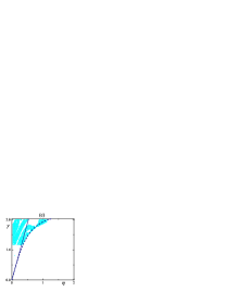
Figure 2: Chaotic regions (dots) in the $\eta-\gamma$ parameter plane corresponding to Eq. (11) with $f(t)=\gamma\cos\left(2\pi t/T\right)$ for three values of the driving period: (a) $T=7.5$, (b) $T=9.38$, (c) $T=10.5$. A dot is plotted on a $100\times 140$ grid when the corresponding maximal LE is greater than $10^{-3}$. Dashed and solid lines represent the theoretical chaotic thresholds [cf. Eqs.(32) and (36), respectively] from GR analysis and MM, respectively.

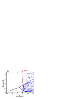
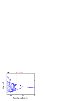
Figure 3: Bifurcation diagrams of Eq. (11) with $f(t)=\gamma\cos\left(2\pi t/T\right)$. (a) Bifurcation diagram of energy $E=\overset{.}{x}^{2}/2+1-\cos x$ as a function of the amplitude $\gamma$ for $\eta=0.95$. The vertical dashed line indicates the threshold amplitude $\gamma_{th}=2.4957$ predicted from Eq. (32). (b) Bifurcation diagram of energy $E=\overset{.}{x}^{2}/2+1-\cos x$ as a function of the damping coefficient $\eta$ for $\gamma=2.4$. The vertical dashed line indicates the threshold value of the damping coefficient $\eta_{th}=0.8514$ predicted from Eq. (32). Fixed parameter: $T=9.38$.

III CONCLUSION

In conclusion, a theory of geometrical resonance in dissipative systems subjected to spatially periodic phase-modulated potentials has been presented, and its effectiveness in obtaining an analytical criterion for the onset of chaotic (homoclinic) instabilities in parameter space beyond the perturbative regime demonstrated by means of a paradigmatic example. From a theoretical point of view, the characterization and determination of the frontiers between chaotic and regular motions of real-world systems is a fundamental problem that needs to be addressed in all branches of science. While the mathematical theory of deterministic chaos was definitively established by the work of Poincaré, Birkhoff, and Smale, the present physical theory suggests understanding the onset of homoclinic chaotic instabilities as being coincident with a critical breaking of the geometrical resonance local symmetry, specifically, as coinciding with a critical breaking of the local conservation of the separatrix’s energy in the co-moving frame for generic spatially periodic phase-modulated potentials. More importantly, the present theory helps to understand the unreasonable effectiveness of the predictions of the Melnikov’s method beyond the perturbative regime. Finally, a natural continuation of the present work is the study of the geometrical resonance local symmetry and its eventual breakage in classical and quantum Hamiltonian systems.

IV ACKNOWLEDGEMENT

The author thanks F. Balibrea, M. Berry, P. Binder, D. Farmer, E. Hernández-García, and P. J. Martínez for discussion and useful comments on an early version of the manuscript. This work was supported by the Ministerio de Ciencia, Innovación y Universidades (MICIU, Spain) through Project No. PID2019-108508GB-100/AEI/10.13039/501100011033 cofinanced by FEDER funds and by the Junta de Extremadura (JEx, Spain) through Project No. GR21012 cofinanced by FEDER funds.

APPENDIX A: DETERMINATION OF THE INITIAL VALUE PROBLEM

From Eqs. (13), (15), (16) with $t_{0}=0$, one obtains

$$f_{GR,0}^{l,r} \equiv f_{GR}^{l,r}\left(t=0\right)=x_{GR}^{l,r}(t=0)-z_{GR}^{l,r}(t=0)=x_{0},$$

$$\overset{.}{f}_{GR,0}^{l} \equiv\overset{.}{f}_{GR}^{i}(t=0)=\overset{.}{x}_{GR}^{l}(t=0)-\overset{.}{z}_{GR}^{l}(t=0)$$

$$=\overset{.}{x}_{0}-2\sqrt{m},$$

$$\overset{.}{f}_{GR,0}^{r} \equiv\overset{.}{f}_{GR}^{r}(t=0)=\overset{.}{x}_{GR}^{r}(t=0)-\overset{.}{z}_{GR}^{r}(t=0)$$

$$=\overset{.}{x}_{0}\mp\frac{2}{\sqrt{m}},$$ (A1)

while from Eq. (18) one obtains

$$C_{1} =x_{0}+\frac{1}{\eta}\left[\overset{.}{x}_{0}-\sum_{n=0}^{\infty}\frac{b_{n}\omega_{n}\cos^{2}\varphi_{n}}{\sin\varphi_{n}}\right]-\sum_{n=0}^{\infty}b_{n}\cos\varphi_{n},$$

$$C_{2} =\frac{1}{\eta}\left[-\overset{.}{x}_{0}+\sum_{n=0}^{\infty}\frac{b_{n}\omega_{n}\cos^{2}\varphi_{n}}{\sin\varphi_{n}}\right],$$ (A2)

for libration motions, and

$$C_{1}^{\prime} =x_{0}+\frac{1}{\eta}\left[\overset{.}{x}_{0}\mp\sum_{n=1}^{\infty}\frac{b_{n}^{\prime}\omega_{n}^{\prime}\cos^{2}\varphi_{n}^{\prime}}{\sin\varphi_{n}^{\prime}}\right]\mp\sum_{n=1}^{\infty}b_{n}^{\prime}\cos\varphi_{n}^{\prime},$$

$$C_{2}^{\prime} =\frac{1}{\eta}\left[-\overset{.}{x}_{0}\pm\sum_{n=1}^{\infty}\frac{b_{n}^{\prime}\omega_{n}^{\prime}\cos^{2}\varphi_{n}^{\prime}}{\sin\varphi_{n}^{\prime}}\right],$$ (A3)

for rotation motions, and where $b_{n},\omega_{n},\varphi_{n},b_{n}^{\prime},\omega_{n}^{\prime},\varphi_{n}^{\prime}$ are given by Eq. (19), while the upper (lower) sign in Eqs. (A1) and (A3) refers to counterclockwise (clockwise) rotations.

APPENDIX B: DERIVATION OF THE GEOMETRICAL RESONANCE EXCITATION FOR THE SEPARATRIX

For the separatrix (27), Eq. (14) reduces to the linear differential equation

$$\overset{..}{f}_{GR}^{s}+\eta\overset{.}{f}_{GR}^{s}=\mp 2\eta\operatorname{sech}\left(t\right).$$ (B1)

After using the method of variation of parameters [27], one straightforwardly obtains the general solution given by Eq. (28) while its derivative is written

$$\overset{.}{f}_{GR}^{s}(t)=-\widetilde{C}_{2}\eta\operatorname{e}^{-\eta t}\mp 4\eta\operatorname{e}^{t}\frac{{}_{2}F_{1}(1,\frac{1+\eta}{2};\frac{3+\eta}{2};-\operatorname{e}^{2t})}{1+\eta}.$$ (B2)

Finally, after taking into account (A1) for $m=1$, i.e., $f_{GR}^{s}(t=0)=x_{0},\overset{.}{f}_{GR}^{s}(t=0)=\overset{.}{x}_{0}\mp 2$, the integration constants are given by,

$$\widetilde{C}_{1} =x_{0}+\frac{1}{\eta}\left(\overset{.}{x}_{0}\mp 2\right),$$

$$\widetilde{C}_{2} =\frac{1}{\eta}\left\{-\overset{.}{x}_{0}\pm 2\mp\eta\left[\psi\left(\frac{3+\eta}{4}\right)-\psi\left(\frac{1+\eta}{4}\right)\right]\right\},$$ (B3)

where $\psi\left(\eta\right)$ is the psi (Digamma) function [22], while the upper (lower) sign in Eqs. (28), (B1), (B2), and (B3) refers to counterclockwise (clockwise) rotations.

APPENDIX C: DERIVATION OF THE THRESHOLD AMPLITUDES FOR THE ONSET OF CHAOTIC INSTABILITIES

Let us consider the simple case of a harmonic excitation $f(t)=\gamma\cos\left(2\pi t/T\right)$.

Libration motions. Equation (26) for $T^{l}\left(m\right)\equiv 4K$ and the Galilean resonance condition $T=T^{l}/(2n+1),n=0,1,...$, reduces to

$$\left\langle\frac{dE}{dt}\right\rangle_{T^{l}}\left(t_{0}\right) =\int_{-2K}^{2K}\left[\eta\overset{.}{z}_{GR}^{l2}-\eta\gamma\omega\overset{.}{z}_{GR}^{l}\sin\left(\omega t\right)\right]dt$$

$$-\int_{-2K}^{2K}\gamma\omega^{2}\overset{.}{z}_{GR}^{l}\cos\left(\omega t\right)dt.$$ (C1)

After substituting $\overset{.}{z}_{GR}^{l}(t;t_{0},m)$ from Eq. (15) into Eq. (C1), using the Fourier series of the elliptic function $\operatorname{cn}\left(\cdot;m\right)$ [18], and using standard tables of integrals [28], one obtains the average energy over the period $T^{l}$ as a function of the initial phase difference $\left(\omega t_{0}\right)$ between the harmonic excitation and the GR solution

$$\left\langle\frac{dE}{dt}\right\rangle_{T^{l}}\left(t_{0}\right) =16\eta\left[E^{\ast}-(1-m)K\right]-\frac{4\pi\gamma\omega\eta\sin\left(\omega t_{0}\right)}{\cosh\left[\omega K^{\prime}\right]}$$

$$-\frac{4\pi\gamma\omega^{2}\cos\left(\omega t_{0}\right)}{\cosh\left[\omega K^{\prime}\right]}.$$ (C2)

From Eq. (C2) one sees that a necessary condition for $\left\langle\frac{dE}{dt}\right\rangle_{T^{l}}\left(t_{0}\right)$ to change sign at some $t_{0}$ is written

$$16\eta\left[E^{\ast}-(1-m)K\right]\leqslant\sqrt{\left(\frac{4\pi\gamma\omega\eta}{\cosh\left[\omega K^{\prime}\right]}\right)^{2}+\left(\frac{4\pi\gamma\omega^{2}}{\cosh\left[\omega K^{\prime}\right]}\right)^{2}},$$ (C3)

where the equals sign in Eq. (C3) yields the threshold amplitude $\gamma_{th}^{l}$ given by Eq. (30).

Rotation motions. Equation (26) for $T^{r}\left(m\right)\equiv$ $2\sqrt{m}K$ and the Galilean resonance condition $T=T^{r}/n$, $n=1,2,...$, reduces to

$$\left\langle\frac{dE}{dt}\right\rangle_{T^{r}}\left(t_{0}\right) =\int_{-\sqrt{m}K}^{\sqrt{m}K}\left[\eta\overset{.}{z}_{GR}^{r2}-\eta\gamma\omega\overset{.}{z}_{GR}^{r}\sin\left(\omega t\right)\right]dt$$

$$-\int_{-\sqrt{m}K}^{\sqrt{m}K}\gamma\omega^{2}\overset{.}{z}_{GR}^{r}\cos\left(\omega t\right)dt.$$ (C4)

After substituting $\overset{.}{z}_{GR}^{r}(t;t_{0},m)$ from Eq. (16) into Eq. (C4), using the Fourier series of the elliptic function $\operatorname*{dn}\left(\cdot;m\right)$ [18], and using standard tables of integrals [28], one obtains the average energy over the period $T^{r}$ as a function of the initial phase difference $\left(\omega t_{0}\right)$ between the harmonic excitation and the GR solution

$$\left\langle\frac{dE}{dt}\right\rangle_{T^{r}}\left(t_{0}\right) =8\eta\sqrt{m}E^{\ast}\mp\frac{2\pi\eta\gamma\omega\sin\left(\omega t_{0}\right)}{\cosh\left[\omega\sqrt{m}K^{\prime}\right]}$$

$$\mp\frac{2\pi\gamma\omega^{2}\cos\left(\omega t_{0}\right)}{\cosh\left[\omega\sqrt{m}K^{\prime}\right]},$$ (C5)

where the upper (lower) sign in Eq. (C5) refers to counterclockwise (clockwise) rotations. From Eq. (C5) one sees that a necessary condition for $\left\langle\frac{dE}{dt}\right\rangle_{T^{r}}\left(t_{0}\right)$ to change sign at some $t_{0}$ is written

$$8\eta\sqrt{m}E^{\ast}\leqslant\sqrt{\left(\frac{2\pi\gamma\omega\eta}{\cosh\left[\omega\sqrt{m}K^{\prime}\right]}\right)^{2}+\left(\frac{2\pi\gamma\omega^{2}}{\cosh\left[\omega\sqrt{m}K^{\prime}\right]}\right)^{2}},$$ (C6)

where the equals sign in Eq. (C6) yields the threshold amplitude $\gamma_{th}^{r}$ given by Eq. (31).

References

- (1) A. J. Lichtenberg and M. A. Lieberman, Regular and Chaotic Dynamics (Springer-Verlag, Berlin, 1991).
- (2) R. Chacón, Phys. Rev. Lett. 77, 482 (1996).
- (3) R. Chacón, Phys. Rev. E 54, 6153 (1996).
- (4) R. Chacón, J. Math. Phys. 38, 1477 (1997).
- (5) J. A. González, B. A. Mello, L. I. Reyes, and L. E. Guerrero, Phys. Rev. Lett. 80, 1361 (1998).
- (6) V. Tereshko and E. Shchekinova, Phys. Rev. E 58, 423 (1998).
- (7) R. Chacón, International Journal of Bifurcation and Chaos 13, 1823 (2003).
- (8) J. A. González, A. Bellorín, L. I. Reyes, C. Vásquez, and L. E. Guerrero, Europhys. Lett. 64, 743 (2003).
- (9) J. A. González, A. Bellorín, L. I. Reyes, C. Vásquez, and L. E. Guerrero, Chaos, Solitons and Fractals 22, 693 (2004).
- (10) T. S. Raju and K. Porsezian, J. Phys. A: Math. Gen. 39, 1853 (2006).
- (11) W. H. Hai, Q. Xie, and S. G. Rong, Eur. Phys. J. D 61, 431 (2011).
- (12) S. Jiménez, J. A. González, and L. Vázquez, International Journal of Bifurcation and Chaos 23, 1350089 (2013).
- (13) M. Ellison et al., Phys. Rev. Lett. 70, 591 (1993).
- (14) K. Staliunas and S. Longhi, Phys. Rev. A 78, 033606 (2008).
- (15) Y. Wei and Y. Lei, Phys. Rev. E 106, 044204 (2022)..
- (16) R. Chacón, P. J. Martínez, and J. A. Martínez, Phys. Rev. E 92, 062921 (2015).
- (17) E. T. Whittaker, A Treatise on the Analytical Dynamics of Particles and Rigid Bodies (Cambridge U.P., New York, 1937), 4th ed.
- (18) P. F. Byrd and M. D. Friedman, Handbook of Elliptic Integrals for Engineers and Scientists (Springer-Verlag, Berlin, 1971).
- (19) R. S. Maier, Phil. Trans. R. Soc. A 366, 1115 (2008).
- (20) H. Li and D. Kusnezov, Phys. Rev. Lett. 83, 1283 (1999).
- (21) J. Guckenheimer and P. Holmes, Nonlinear Oscillations, Dynamical Systems, and Bifurcations of Vector Fields (Springer-Verlag, New York, 1983).
- (22) M. Abramowitz and I. A. Stegun, Handbook of Mathematical Functions (Dover, New York, 1972).
- (23) V. K. Melnikov, Tr. Mosk. Ova 12, 3 (1963) [Trans. Moscow Math. Soc. 12A, 1 (1963)].
- (24) H. J. Poincaré, Les Méthodes Nouvelles de la Mécanique Céleste (Gauthier-Villars, Paris, 1899).
- (25) A. Wolf, J. B. Swift, H. L. Swinney, and J. A. Vastano, Physica D 16, 285 (1985).
- (26) H. J. Poincaré, Acta Mathematica 13, 1 (1890).
- (27) E. L. Ince, Ordinary Differential Equations (Dover, New York, 1956).
- (28) I. Gradshteyn and I. Ryzhik, Table of Integrals, Series and Products (Academic, New York, 1994).
- (29) R. Chacón, Control of Homoclinic Chaos by Weak Periodic Perturbations (World Scientific, Singapore, 2005).