Quantum Quenches in Chern Insulators

Abstract

We explore the non-equilibrium response of Chern insulators. Focusing on the Haldane model, we study the dynamics induced by quantum quenches between topological and non-topological phases. A notable feature is that the Chern number, calculated for an infinite system, is unchanged under the dynamics following such a quench. However, in finite geometries, the initial and final Hamiltonians are distinguished by the presence or absence of edge modes. We study the edge excitations and describe their impact on the experimentally-observable edge currents and magnetization. We show that, following a quantum quench, the edge currents relax towards new equilibrium values, and that there is light-cone spreading of the currents into the interior of the sample.

Topological phases of matter display many striking features, ranging from the precise quantization of macroscopic properties, to the emergence of fractional excitations and gapless edge states. An important class of topological systems is provided by the so-called Chern insulators realized in two-dimensional settings Thouless et al. (1982). A famous example is the Haldane model Haldane (1988), which describes spinless fermions hopping on a honeycomb lattice. The Haldane model exhibits both topological and non-topological phases, and its behavior is closely related to the integer quantum Hall effect. Recent advances using ultra cold atoms Goldman et al. (2009); Alba et al. (2011); Aidelsburger et al. (2013); Goldman et al. (2013a); Wright (2013) have led to the experimental realization of the Haldane model Jotzu et al. (2014). Proposals also exist for realizing other states of topological matter using cold atoms Setiawan et al. (2015).

A fundamental characteristic of topological systems is their robustness to local perturbations, making them ideal candidates for applications in metrology and quantum computation. However, much less is known about their dynamical response to global perturbations and time-dependent driving. This issue is of relevance in a variety of contexts, ranging from the time-evolution and controlled manipulation of prepared topological states, to the dynamics of topological systems coupled to their environment. Understanding the impact of topology on the out of equilibrium response is crucial for further developments, and is the motivation for this present work. For recent progress in this direction see Refs. Dóra and Moessner (2011); Uehlinger et al. (2013); Barnett (2013); Patel et al. (2013); Kells et al. (2014); Dutta et al. (2010); Hauke et al. (2014); Stojchevska et al. (2014).

In this manuscript we investigate the non-equilibrium dynamics of the paradigmatic Haldane model. In particular, we consider quantum quenches and sweeps between topological and non-topological phases. Key questions that we will address include: What happens to the topological properties on transiting between different phases? What happens to the edge excitations following a quantum quench? How do the topological characteristics influence the non-equilibrium dynamics?

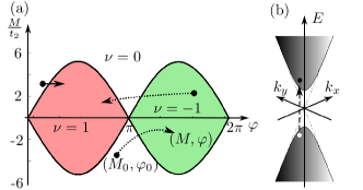
Figure 1: (a) Phase diagram of the Haldane model obtained from the low-energy Dirac fermion representation, showing topological ($\nu=\pm 1$) and non-topological phases ($\nu=0$) Haldane (1988). We consider quantum quenches and sweeps between different regions of the phase diagram, as illustrated by the arrows. (b) The low-energy spectrum of the Haldane model is described by excitations around two Dirac points. After a quench, carriers in the lower band are excited to the upper band.

Model.— The Haldane model describes spinless fermions hopping on a honeycomb lattice with both nearest and next nearest neighbor hopping parameters. The Hamiltonian is given by Haldane (1988)

$$\hat{H}=t_{1}\sum_{\langle i,j\rangle}\left(\hat{c}^{{\dagger}}_{i}\hat{c}^{\mathstrut}_{j}+\mbox{h.c.}\right)\\ +t_{2}\sum_{\langle\!\langle i,j\rangle\!\rangle}\left(e^{\mathrm{i}\varphi_{ij}}\hat{c}^{{\dagger}}_{i}\hat{c}^{\mathstrut}_{j}+\mbox{h.c.}\right)\\ +M\sum_{i\in A}\hat{n}_{i}-M\sum_{i\in B}\hat{n}_{i},$$ (1)

where the fermionic operators obey the anticommutation relations $\{\hat{c}_{j},\hat{c}_{j}^{\dagger}\}=\delta_{ij}$ and $\hat{n}_{i}\equiv\hat{c}_{i}^{\dagger}{\hat{c}_{i}}$. Here, $\langle i,j\rangle$ and $\langle\!\langle i,j\rangle\!\rangle$ indicate the summation over the nearest and next to nearest neighbor sites respectively, and $A$ and $B$ label the two sub-lattices. The phase factor $\varphi_{ij}=\pm\varphi$ is introduced in order to break time-reversal symmetry and is positive for anticlockwise next to nearest neighbor hopping. The energy off-set $\pm M$ breaks spatial inversion symmetry. The phase diagram of the Haldane model is shown in Fig. 1 (a); following Ref. Haldane (1988) we assume that $|t_{2}/t_{1}|\leq 1/3$ so that the bands may touch, but not overlap.

For $t_{2},M\ll t_{1}$, the Hamiltonian (1) has a linear dispersion near the six corners of the hexagonal Brillouin zone, but only two of these are inequivalent. As a result, close to half-filling, the low-energy description is given by the sum of two Dirac Hamiltonians

$$\hat{H}_{\alpha}=\begin{pmatrix}m_{\alpha}c^{2}&-c\,k\,e^{\mathrm{i}\alpha\theta}\\ -c\,k\,e^{-\mathrm{i}\alpha\theta}&-m_{\alpha}c^{2}\end{pmatrix},$$ (2)

where $\alpha=\pm 1$ label the Dirac points. Here, $c=3t_{1}/2\hbar$ is the effective speed of light, $k\exp(\mathrm{i}\theta)$ parameterizes the 2D momentum $(k_{x},k_{y})$ and $m_{\alpha}=(M-3\sqrt{3}\alpha t_{2}\sin\varphi)/c^{2}$ is the effective mass Haldane (1988). The topological phases have a non-vanishing Chern number $\nu$ Chern (1946); Thouless et al. (1982); Berry (1984); Haldane (1988). For a state $|\psi\rangle$ this is defined by the integral of the Berry curvature over the 2D Brillouin zone

$$\nu=\frac{1}{2\pi}\int d^{2}k\,\Omega,$$ (3)

where $\Omega=\partial_{k_{x}}A_{k_{y}}-\partial_{k_{y}}A_{k_{x}}$ and $A_{k_{\mu}}=\mathrm{i}\Braket{\psi}{\partial_{k_{\mu}}}{\psi}$ is the Berry connection. For the ground state of the Haldane model $\nu\in\pm 1,0$. This may be decomposed into contributions from the two Dirac points as $\nu=\nu_{+}+\nu_{-}$, where $\nu_{\alpha}=-\tfrac{\alpha}{2}\,{\rm sign}(m_{\alpha})\in\pm 1/2$. The boundaries of the topological phases correspond to the locations where $m_{\pm}$ changes sign. They are thus given by $M/t_{2}=\pm 3\sqrt{3}\sin\varphi$, and are independent of $t_{1}$; see Fig. 1.

Quantum Quenches.— In order to gain insight into the non-equilibrium dynamics of the Haldane model, we consider quantum quenches between different points $(M,\varphi)$ on the phase diagram shown in Fig. 1, for fixed values of $t_{1}$ and $t_{2}$. At time $t=0$, we prepare our system in the ground state with parameters $(M_{0},\varphi_{0})$. At half-filling our initial state fills the lower band. We then abruptly change the parameters of $\hat{H}$ to $(M,\varphi)$, and allow the system to evolve unitarily under the action of this new Hamiltonian. In general, this will lead to a non-trivial occupation of both the lower and the upper bands.

We begin by examining the non-equilibrium response of the effective Dirac Hamiltonian ${\hat{H}}={\hat{H}}_{+}+{\hat{H}}_{-}$. Since $\nu=-\tfrac{1}{2}\left[{\rm sign}(m_{+})-{\rm sign}(m_{-})\right]$, quenching between different phases corresponds to changing the sign of one or both of the masses $m_{\alpha}$. For a given Dirac point, such changes will lead to a re-distribution of carriers between the two bands. For a $\theta$ independent superposition, $\Ket{\psi_{\alpha}(k)}=a_{\alpha}(k)e^{-\mathrm{i}E_{\alpha}^{l}(k)t}\Ket{l_{\alpha}(k)}+b_{\alpha}(k)e^{-\mathrm{i}E_{\alpha}^{u}(k)t}\Ket{u_{\alpha}(k)}$, the Chern number is formally given by

$$\nu_{\alpha}(t)=-\alpha\operatorname{sign}m_{\alpha}\left(\frac{1}{2}-\lvert b_{\alpha}(0)\rvert^{2}\right)\\ -\lvert b_{\alpha}(\infty)\rvert\lvert a_{\alpha}(\infty)\rvert\cos[(E_{\alpha}^{u}(\infty)-E_{\alpha}^{l}(\infty))t+\delta].$$ (4)

Here, $a_{\alpha}(k)$ and $b_{\alpha}(k)$ are complex $c$-numbers, $\delta={\rm arg}(a_{\alpha}(\infty))-{\rm arg}(b_{\alpha}(\infty))$, and $E_{\alpha}^{l,u}(k)$ are the energies in the lower and upper bands. In general, $\nu_{\alpha}(t)$ is time-dependent, and differs from its ground state values $\pm 1/2$. However, the time-dependence only enters via the superposition coefficients evaluated at $k=\infty$. An explicit computation shows that $b_{\alpha}(\infty)=0$, following a quantum quench; see Fig. 2 and the Supplemental Material. In addition, $b_{\alpha}(0)=0,\pm 1$, so the potential modification of $\nu_{\alpha}$ is compensated by the change in sign of $m_{\alpha}$.

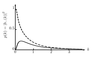
Figure 2: Probability of occupying the upper band for a single Dirac point ($\alpha=-1$) with $c=1$, following a quench of $m_{\alpha}$. Sign-preserving quench, $m_{-}=-1\rightarrow m_{-}^{\prime}=-0.1$ (solid line) and a sign-changing quench, $m_{-}=-1\rightarrow m_{-}^{\prime}=0.1$ (dashed line). In both cases, $b_{-}(\infty)=0$, corresponding to the time-independence of $\nu_{-}(t)$ using Eq. (4). The sign-changing quench yields $|b_{-}(0)|^{2}=1$, but the contribution to $\nu_{-}(t)$ in Eq. (4) is compensated by the change in sign of $m_{-}$. As a result, $\nu_{-}$ is unchanged from its initial value.

As a result the Chern number is unchanged from its initial value, even if one quenches between different phases. Similar results may also be obtained for a linear sweep, $m_{\alpha}(t)=t/\tau$; see Supplemental Material.

Preservation of Chern Number.— An intuitive way to understand the persistence of $\nu$ following a quantum quench is in terms of spin-textures in momentum space. The Dirac Hamiltonian in Eq. (2) can be recast as an effective spin in a ${\bf k}$-dependent magnetic field, ${\bf h}_{\alpha}({\bf k})$. Explicitly, $\hat{H}_{\alpha}({\bf k})\equiv-{\bf h}_{\alpha}({\bf k})\cdot{\bm{\sigma}}/2$, where ${\bm{\sigma}}$ are the Pauli matrices. In equilibrium, the topological phases with $\nu_{\alpha}=\pm 1/2$ correspond to meron spin configurations which wind on the upper (lower) half-sphere Fradkin (2013). Following a quantum quench, the spins precess in the effective magnetic field of the new Hamiltonian, preserving the topological characteristics of the initial spin configuration. A similar argument may also be applied to the Haldane model (1) in ${\bf k}$-space. Indeed, one expects the preservation of topological invariants under time evolution to be a general feature for non-interacting fermions in a periodic system, where each ${\bf k}$-state evolves unitarily under some Hamiltonian $\hat{H}({\bf k})$, provided $\hat{H}({\bf k})$ is smoothly varying in ${\bf k}$-space.

Edge States.— In the above discussion we have demonstrated that the value of $\nu$ is unchanged as one quenches and sweeps between different phases. However, there is a fundamental distinction between the topological and non-topological phases, due to the presence or absence of edge states in a finite-size sample Hao et al. (2008). In quenching between phases of different topological character, these edge states will either appear or disappear, depending on the direction of the quench. This is confirmed in Fig. 3, which shows the re-construction and re-population of the energy levels following a quench from the non-topological phase to a topological phase.

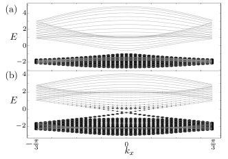
Figure 3: Energy spectrum of the Haldane model obtained by exact diagonalization on a finite-size strip of width $N=20$ unit cells with armchair edges. We take periodic (open) boundary conditions along (transverse to) the strip and set $t_{1}=1$, $t_{2}=\frac{1}{3}$, and $M=1$. (a) Equilibrium population of the energy levels in the non-topological phase with $\varphi=\frac{\pi}{6}$. (b) Re-population of the levels after a quench to the topological phase with $\varphi=\frac{\pi}{3}$, corresponding to the solid arrow in Fig. 1 (a). The size of the dots is proportional to the probability of finding a particle in the mode. Post-quench, the filling of the edge states and the bands is non-trivial.

It is readily seen that the edge states emerge and are populated as a result of the quench, in spite of the fact that $\nu$ remains equal to zero in the absence of boundaries. Conversely, a quench from a topological phase to the non-topological phase eliminates the edge states, whilst $\nu$ remains pinned at unity.

Edge Currents and Orbital Magnetization.— Having examined the re-population of the edge states we now consider physical observables that depend on these states, including the edge currents and the orbital magnetization. We first consider these quantities in equilibrium, which already display interesting features. We define the local current flowing through the site $i$ by $\hat{{\bf J}}_{i}=-\frac{{\rm i}}{2}\sum_{j}{\bm{\delta}}_{ji}(t_{ij}\hat{c}^{\dagger}_{i}\hat{c}_{j}-{\rm h.c.})$, where $t_{ij}$ is the hopping parameter of the Haldane model between sites $i$ and $j$, ${\bm{\delta}}_{ji}$ is the vector displacement of site $i$ from $j$, and the sum is over the nearest and next nearest neighbors. The site indices may be decomposed into the triplet $\{m,n,s\}$ labeling the $x$ and $y$ positions of the unit cell and the sublattice index $s=A,B$. The total longitudinal current flowing along the strip in the $x$-direction at a definite transverse $y$-position is therefore given by $J_{n}^{x}=\langle\hat{J}^{x}_{n}\rangle=\sum_{ms}\langle{\hat{J}^{x}_{mns}}\rangle$.

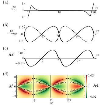
Figure 4: Equilibrium properties of the Haldane model on a finite-size strip as used in Fig. 3. (a) Total longitudinal current $J_{n}^{x}$ along the strip as a function of the transverse spatial index $n\in 1,\dots,20$, for $M=0$ and $\varphi=\pi/3$. (b) Edge currents corresponding to $J_{n}^{x}$ with $n=1$ (solid) and $n=20$ (dashed) for $M=0$. The edge currents exhibit $\pi$-periodicity in $\varphi$ and vanish when $\varphi=\pi/2$. (c) Orbital magnetization ${\bm{\mathcal{M}}}$ as a function of $\varphi$ for $M=0$. (d) Intensity plot of ${\bm{\mathcal{M}}}$ where the dashed lines correspond to the boundaries of the topological phases. Numerically we observe that ${\bm{\mathcal{M}}}$ vanishes on the loci $M=\pm\sin\varphi$ (solid) within the topological phases. The loci are fits to the numerical data (triangles) where ${\bm{\mathcal{M}}}=0$. The magnetization also vanishes on the vertical lines $\varphi=\pi/2,\pi,3\pi/2,\dots$ as follows from symmetry considerations.

In Fig. 4(a) we plot this current within the topological phase for $M=0$ and $\varphi=\pi/3$. The presence of the counter-propagating edge currents is readily seen. In Fig. 4(b) we show the dependence of these edge currents on $\varphi$. Somewhat surprisingly, the edge currents vanish within the topological phase, in spite of the presence of edge states in the spectrum. The edge currents are composed of counter-propagating contributions which cancel at $\varphi=\pi/2$; see Supplemental Material. Moreover, the longitudinal currents $J_{n}^{x}$ exhibit $\pi$-periodicity in $\varphi$. This is a consequence of being at half-filling and occurs in spite of the fact that the Hamiltonian and the current operator have a periodicity of $2\pi$. To prove the $\pi$-periodicity in $\varphi$ we first note that both the Hamiltonian and the current operator change sign under the transformation $M\rightarrow-M$, $\varphi\rightarrow\varphi+\pi$, $\hat{c}_{mnA}\rightarrow\hat{c}_{mnA}$, $\hat{c}_{mnB}\rightarrow-\hat{c}_{mnB}$, thereby interchanging the upper and the lower bands. At half-filling, we fill only the lower band, and it follows that $J_{n}^{x}(M,\varphi)=J_{n}^{x}(-M,\varphi+\pi)$. In addition, the current changes sign under the parity transformation $x\rightarrow-x$. This interchanges the sublattices and corresponds to $M\rightarrow-M$ and $\varphi\rightarrow-\varphi$. It follows that $J_{n}^{x}(M,\varphi)=-J_{n}^{x}(-M,-\varphi)=J_{n}^{x}(-M,\varphi)$, where in the last step we use the transformation properties under time-reversal. Combining these relations, one obtains the $\pi$-periodicity in $\varphi$ and the vanishing of the longitudinal currents for $\varphi=\pi/2$.

Similar arguments also apply to the (lattice discretization of the) orbital magnetization:

$${\bm{\mathcal{M}}}=\frac{1}{2{\mathcal{A}}}\int d^{2}r\,{\bf r}\times\langle\hat{\bf J}({\bf r})\rangle,​$$ (5)

where $\hat{\bf J}({\bf r})$ is the local current density operator and ${\mathcal{A}}$ is the area. As shown in Fig. 4(c) this also vanishes within the topological phases and has $\pi$-periodicity in $\varphi$ Thonhauser et al. (2005); Ceresoli et al. (2006). Our numerical computations also reveal that the magnetization vanishes on a sinusoidal locus $M=\pm\sin(\varphi)$ within the topological phases; see Fig. 4(d). In addition, ${\bm{\mathcal{M}}}(M,\varphi)$ has extrema at $M=0$ and on the topological phase boundaries, $M=\pm\sqrt{3}\sin(\varphi)$, for fixed $\varphi$. Away from half-filling, the particle-hole symmetry is broken and the periodicity of the currents and the magnetization is restored to $2\pi$. The increase or decrease of the edge currents depends on the sign of the doping and the Chern index; see Supplemental Material.

Dynamics of the Edge Currents.— Having discussed the equilibrium properties of the edge currents we now consider their response to quantum quenches. In Fig. 5 we show quenches from the topological to the non-topological phase. The edge currents decay towards new values that are found to be numerically close to the equilibrium values of the post-quench Hamiltonian. This is in spite of the fact that the system is left in an excited state under unitary evolution, and that $\nu$ remains pinned to unity in the absence of boundaries. Quenches from the non-topological to topological phases exhibit similar behavior; see Supplemental Material.

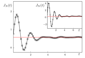
Figure 5: Dynamics of the edge current $J_{N}^{x}(t)$ for $N=30$ (circles) and $N=40$ (crosses) following a quantum quench between the topological phase and the non-topological phase with $t_{1}=1$, $t_{2}=\frac{1}{3}$ and fixed $\varphi=\pi/3$. Quenches from $M=1.4$ to $M=1.6$ (main panel) and from $M=1.4$ to $M=2.2$ (inset) showing that the edge currents approach new equilibrium values. For the chosen parameters, these are very close to the ground state expectation values of $J_{N}^{x}$ in the final Hamiltonian, as indicated by the horizontal lines.

Further insight into the non-equilibrium evolution may be gleaned from the time-evolution of the longitudinal currents across the two-dimensional system. As shown in Fig. 6, the damped oscillations of the edge currents is accompanied by the light-cone spreading of the currents into the interior of the sample. It would be interesting to observe this dynamics in experiment, which is in principle possible if local imaging is available Goldman et al. (2013b).

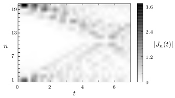
Figure 6: Dynamics of the currents $\left|J_{n}^{x}(t)\right|$ following a quantum quench from the topological to the non-topological phase for the parameters used in the inset of Fig. 5. The damped oscillations of the edge currents are clearly visible, as is the light-cone spreading of the currents into the interior of the sample, where $c=3t_{1}/2\hbar=3/2$ is the effective speed of light. The waves propagating from the two edges meet at time $t\sim(N/2)\sqrt{3}/2c\sim 5.77$, leading to resurgent oscillations in finite-size samples; see Supplemental Information.

Conclusions.— In this manuscript we have explored the non-equilibrium dynamics of the Haldane model. We have demonstrated that the Chern number is preserved in both quenches and sweeps between different regions of the phase diagram. However, the edge states may be re-constructed and re-populated leading to changes in the accompanying edge currents. Predictions for experiment include the vanishing of the equilibrium edge currents in the topological phases, and the light-cone spreading of the currents following a quantum quench. There are a wide variety of directions for further research, including the dynamics of the conductivity and its relation to the Chern number, and the role of decoherence via coupling to the environment.

Acknowledgements.— This work was supported by EPSRC Grants EP/J017639/1 and EP/K030094/1. MJB thanks the EPSRC Centre for Cross-Disciplinary Approaches to Non-Equilibrium Systems (CANES) funded under grant EP/L015854/1. MJB and MDC thank the Thomas Young Center.

Whilst this work was in preparation the pre-print D’Alessio and Rigol (2014) appeared, which reaches similar conclusions to ours regarding the invariance of $\nu$ under unitary evolution.

I Supplemental Material

Haldane Model.— For completeness, let us recall some details of the Haldane model Haldane (1988). A key feature is the presence of time-reversal symmetry breaking induced by the complex second-neighbor hopping. In Haldane’s original paper this corresponds to a staggered magnetic field, where the local flux within a hexagonal plaquette is non-zero, but the total flux through a plaquette vanishes. In the experimental realization of Ref. Jotzu et al. (2014) this is achieved by circular modulation of the lattice position. In Fourier space, the Hamiltonian is given by Haldane (1988)

$$H(\mathbf{k})=2t_{2}\cos\varphi\left(\sum_{i}\cos(\mathbf{k}\cdot\mathbf{b}_{i})\right){\rm I}\\ +t_{1}\left(\sum_{i}[\cos(\mathbf{k}\cdot\mathbf{a}_{i})\sigma^{1}+\sin(\mathbf{k}\cdot\mathbf{a}_{i})\sigma^{2}]\right)\\ +\left[M-2t_{2}\sin\varphi\left(\sum_{i}\sin(\mathbf{k}\cdot\mathbf{b}_{i})\right)\right]\sigma^{3},$$ (6)

where $\sigma^{\mu}$ are Pauli matrices and ${\rm I}$ is the identity matrix. Here, $\mathbf{a}_{1},\mathbf{a}_{2},\mathbf{a}_{3}$ are the displacements from a $B$ site to its three nearest-neighbor $A$ sites. The $\mathbf{b}_{i}$’s are defined via cyclic permutations of $\mathbf{b}_{1}:=\mathbf{a}_{2}-\mathbf{a}_{3}$ and correspond to the second-neighbor displacements, $\pm\mathbf{b}_{i}$. For $M=0$ and $\varphi=0$, the two bands touch at the six corners of the Brillouin Zone. However, only two of these points are inequivalent, and we denote these by $\mathbf{k}_{\alpha}$ with $\alpha=\pm$. Expanding the Hamiltonian around these two corners, with $\bm{\Pi}_{\alpha}=(\Pi^{x}_{\alpha},\Pi^{y}_{\alpha})=\mathbf{k}-\mathbf{k}_{\alpha}$, one obtains Haldane (1988)

$$H_{\alpha}=c(\Pi^{1}_{\alpha}\sigma^{2}-\Pi^{2}_{\alpha}\sigma^{1})+m_{\alpha}c^{2}\sigma^{3},$$ (7)

where $m_{\alpha}$ and $c$ defined following Eq. (2) and

$$(\Pi^{1}_{\alpha}+\mathrm{i}\Pi^{2}_{\alpha})=\frac{2}{3}\sum_{i}e^{\mathrm{i}\mathbf{k}_{\alpha}\cdot\mathbf{a}_{i}}\frac{\mathbf{a}_{i}\cdot\bm{\Pi}_{\alpha}}{\lvert\mathbf{a}_{i}\rvert}.$$ (8)

In order to connect with the notations used in Eq. (2) we parameterize the complex number $\Pi^{2}_{\alpha}+\mathrm{i}\Pi^{1}_{\alpha}$ as $ke^{\mathrm{i}\alpha\theta}$.

Berry Phase.— In a gauge theory, invariant under a local transformation $\Ket{\psi^{\prime}(\mathbf{X})}:=e^{-\mathrm{i}\rho(\mathbf{X})}\Ket{\psi(\mathbf{X})}$, parameterized by $\mathbf{X}$, one may define a covariant derivative

$$\Ket{D_{\mu}\psi(\mathbf{X})}=\Ket{\partial_{\mu}\psi(\mathbf{X})}-\Ket{\psi(\mathbf{X})}\Braket{\psi(\mathbf{X})}{\partial_{\mu}\psi(\mathbf{X})},$$ (9)

where $\Ket{\psi(\mathbf{X})}\Bra{\psi(\mathbf{X})}$ projects out the parts of $\Ket{\partial_{\mu}\psi(\mathbf{X})}$ that are not orthogonal to $\Ket{\psi(\mathbf{X})}$. One may also introduce the Berry connection $A_{\mu}(\mathbf{X})=\mathrm{i}\Braket{\psi(\mathbf{X})}{\partial_{\mu}\psi(\mathbf{X})}$, the Berry phase $\phi$, for a closed path $\Gamma$ in parameter space $e^{\mathrm{i}\phi}:=e^{\mathrm{i}\oint_{\Gamma}\mathop{}\!\mathrm{d}X^{\mu}A_{\mu}(\mathbf{X})}$, and the Berry curvature $\Omega_{\mu\sigma}=\Braket{D_{\mu}\psi(\mathbf{X})}{D_{\sigma}\psi(\mathbf{X})}-\Braket{D_{\sigma}\psi(\mathbf{X})}{D_{\mu}\psi(\mathbf{X})}$. One may also generalize the Gauss–Bonnet theorem:

$$\nu:=\frac{\phi}{2\pi}=\frac{1}{2\pi}\int_{M_{2}}\mathop{}\!\mathrm{d}X^{\mu}\wedge\mathop{}\!\mathrm{d}X^{\sigma}\,\Omega_{\mu\sigma}(\mathbf{X})\in{\mathbb{Z}},$$ (10)

where $M_{2}$ is a closed orientable 2-manifold and $\nu$ is the Chern number.

Chern Number for Dirac Points.— For the Dirac Hamiltonian, given by Eq. (2) with $\alpha=-1$ say, the Berry connection is given by $A_{k}^{-}=\mathrm{i}\Braket{\psi}{\partial_{k}\psi}$ and $A_{\theta}^{-}=\mathrm{i}\Braket{\psi}{\partial_{\theta}\psi}$, where we parameterize the momentum-space 2-manifold $M_{2}$ by $(k,\theta)$. For a superposition of the form

$$\Ket{\psi(k,\theta)}=a(k)\Ket{l(k,\theta)}+b(k)\Ket{u(k,\theta)},$$ (11)

where $|l\rangle$ and $|u\rangle$ correspond to the lower and upper band eigenstates, $A_{k}^{-}$ and $A_{\theta}^{-}$ are independent of $\theta$. As a result, the contribution of this Dirac point to the Chern number, $\nu=\nu_{+}+\nu_{-}$, is

$$\nu_{-}=\frac{1}{2\pi}\int_{0}^{2\pi}\mathop{}\!\mathrm{d}\theta\int_{0}^{\infty}\mathop{}\!\mathrm{d}k\,\Omega^{-}=\int_{0}^{\infty}\mathop{}\!\mathrm{d}k\,\partial_{k}A_{\theta}^{-}=\left.A_{\theta}^{-}\right|_{0}^{\infty},$$ (12)

where $\Omega^{-}=\partial_{k}A^{-}_{\theta}-\partial_{\theta}A_{k}^{-}$. Using the explicit forms

$$\Ket{l}=\begin{pmatrix}e^{-\mathrm{i}\theta}f_{-}(k,m_{-})\\ f_{+}(k,m_{-})\end{pmatrix},\quad\Ket{u}=\begin{pmatrix}-e^{-\mathrm{i}\theta}f_{+}(k,m_{-})\\ f_{-}(k,m_{-})\end{pmatrix}$$ (13)

where $f_{\pm}(k,m):=\sqrt{\frac{1}{2}\left(1\pm\frac{m_{-}}{\sqrt{k^{2}+m_{-}^{2}}}\right)}$, one obtains

$$A_{\theta}^{-}=\lvert a(k)\rvert^{2}f_{-}^{2}(k,m_{-})+\lvert b(k)\rvert^{2}f_{+}^{2}(k,m_{-})\\ -\frac{k}{2\sqrt{k^{2}+m_{-}^{2}}}\left(a^{*}(k)b(k)+{\rm h.c.}\right).$$ (14)

It follows that

$$A_{\theta}^{-}(\infty) =\frac{1}{2}\left[1-\left(a^{*}(\infty)b(\infty)+{\rm h.c.}\right)\right]$$ (15)

$$A_{\theta}^{-}(0) =\begin{cases}\lvert b(0)\rvert^{2}&m_{-}>0\\ \lvert a(0)\rvert^{2}&m_{-}<0.\end{cases}$$ (16)

Eq. (4) follows by reinstating the time dependence $a(k)\rightarrow a(k)e^{-\mathrm{i}E_{l}t}$ and $b(k)\rightarrow b(k)e^{-\mathrm{i}E_{u}t}$, for unitary evolution under the Dirac Hamiltonian.

Quench.— We now consider a quench $m_{-}\rightarrow m_{-}^{\prime}$. The system is initially prepared in the ground state of $H_{-}(m_{-})$, corresponding to the filled lower band, $\Ket{l}$. Immediately after the quench we may decompose $\Ket{l}$ into the eigenstates of the post-quench Hamiltonian:

$$a(k) =f_{-}(k,m_{-})f_{-}(k,m_{-}^{\prime})+f_{+}(k,m_{-})f_{+}(k,m_{-}^{\prime}),$$

$$b(k) =f_{+}(k,m_{-})f_{-}(k,m_{-}^{\prime})-f_{-}(k,m_{-})f_{+}(k,m_{-}^{\prime}).$$

The probability of being in the upper band, $|b_{-}(k)|^{2}$ is plotted in Fig. 2. In particular, one obtains $b(\infty)=0$ and $b(0)=0$ ($b(0)=\pm 1$) for sign-preserving (sign-changing) mass quenches. The preservation of the contribution to the Chern number is discussed in the main text.

Linear Sweep.— We extend the results for the Chern number preservation to linear, time-dependent, sweeps. We again consider $\alpha=-$ and set $m_{-}=\frac{t}{\tau}$ in Eq. (2), corresponding to a sign changing sweep over the interval $t\in[-\infty,\infty]$. We prepare the system in the ground state at $t=-\infty$ and track the subsequent evolution Dutta et al. (2010). At any instant of time the state can be written as a superposition over the eigenstates of $H_{-}(t)$:

$$\Ket{\psi(k,\theta,t)}=a(k,t)\Ket{l(k,\theta,t)}+b(k,t)\Ket{u(k,\theta,t)}.$$ (17)

Using Eq. (12) and Eq. (14) one obtains

$$\nu_{-}(t)=\operatorname{sign}t\left(\frac{1}{2}-\lvert b(0,t)\rvert^{2}\right)\\ +\left[\lim_{k\rightarrow\infty}-\lim_{k\rightarrow 0}\right]\left[\frac{k}{2\sqrt{k^{2}+\frac{t^{2}}{\tau^{2}}}}(a^{*}(k,t)b(k,t)+\mbox{h.c.})\right].$$ (18)

We now need to evaluate the coefficients $a$ and $b$ for $k=0$ and $k=\infty$. For $k=0$ the eigenstates of $H_{-}(t)$ are

$$\Ket{l(0,t)} =\begin{pmatrix}e^{-\mathrm{i}\theta}\sqrt{\frac{1}{2}(1-\operatorname{sign}{t})}\\ \sqrt{\frac{1}{2}(1+\operatorname{sign}{t})}\end{pmatrix},$$ (19)

$$\Ket{u(0,t)} =\begin{pmatrix}-e^{-\mathrm{i}\theta}\sqrt{\frac{1}{2}(1+\operatorname{sign}{t})}\\ \sqrt{\frac{1}{2}(1-\operatorname{sign}{t})}\end{pmatrix}.$$ (20)

These are time-independent for $t\neq 0$, and for $k=0$ the system remains in the lower band up to $t=0^{-}$. At $t=0^{+}$ the mass parameter changes sign, and at $k=0$, overlaps completely with the upper band:

$$\lvert\Braket{l(0,0^{-})}{u(0,0^{+})}\rvert=1.$$

Henceforth, the $k=0$ mode remains in the upper band. At $k=\infty$ the eigenstates are independent of time:

$$\Ket{l(\infty,t)} =\begin{pmatrix}e^{-\mathrm{i}\theta}\sqrt{\frac{1}{2}}\\ \sqrt{\frac{1}{2}}\end{pmatrix},$$ (21)

$$\Ket{u(\infty,t)} =\begin{pmatrix}-e^{-\mathrm{i}\theta}\sqrt{\frac{1}{2}}\\ \sqrt{\frac{1}{2}}\end{pmatrix}.$$ (22)

The system remains in the lower band for $k=\infty$. Summarizing, one obtains

$$\lvert b(0,t)\rvert=\begin{cases}0,&t<0\\ 1,&t>0\end{cases}\quad{\rm and}\quad\lvert b(\infty,t)\rvert=0\quad\forall t.$$ (23)

This parallels the situation for the quench protocol as shown by the dashed line in Fig. 2. The preservation of $\nu_{-}$ follows by substituting Eq. (23) into Eq. (18).

Preservation of Chern Number.— Having established the preservation of $\nu$ using the low-energy Dirac Hamiltonian, we examine the non-equilibrium response of the Haldane model. By recasting Eq. (3) in the form

$$\nu=\frac{1}{2\pi}\oint_{\partial{\rm BZ}}\mathop{}\!\mathrm{d}k^{\mu}A_{k_{\mu}},$$ (24)

we may focus on the time-dependence of the Berry connection. In general, $\dot{A}_{k_{\mu}}=i\langle\dot{\psi}|\partial_{k_{\mu}}|\psi\rangle+i\langle\psi|\partial_{k_{\mu}}|\dot{\psi}\rangle=\langle\psi|[\partial_{k_{\mu}},\hat{H}]|\psi\rangle$, or equivalently, $\dot{A}_{k_{\mu}}=\langle\psi|(\partial_{k_{\mu}}\hat{H})|\psi\rangle$. Expanding the initial state $|\psi\rangle=\sum_{\gamma=l,u}c_{\gamma}e^{-iE_{\gamma}t}|\gamma\rangle$ in terms of the eigenstates $|\gamma\rangle$ of the final Hamiltonian

$$\dot{A}_{k_{\mu}}(k_{x},k_{y})=\sum_{\gamma=l,u}c_{\gamma}c_{\gamma^{\prime}}^{\ast}\langle\gamma^{\prime}|\partial_{k_{\mu}}\hat{H}|\gamma\rangle e^{i(E_{\gamma^{\prime}}-E_{\gamma})t}.$$ (25)

In general, this is time-dependent. However, using the symmetries of the final Hamiltonian, the components of $\dot{A}_{k_{\mu}}$ along the Brillouin zone boundary occur in equal pairs and cancel in the line integral for $\dot{\nu}$. For example, within the upper and lower triangles depicted in Fig. 7, $\hat{H}(k_{x},k_{y})=\hat{H}^{*}(k_{x},-k_{y})$. Periodicity in $k$-space ensures that $\hat{H}(k_{x},k_{y})=\hat{H}(k_{x},-k_{y})$ along the corresponding zone boundaries, so that $\hat{H}$ is real on these segments.

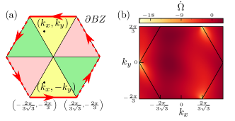
Figure 7: First Brillouin zone of the Haldane model. (a) In each of the triangles the Berry connection and the Berry curvature are time-dependent. However, the Chern number is given by the line integral of the Berry connection along the zone boundary, as indicated by the arrows. Following a quench, the time-dependent contributions to $\nu$ from opposite sides of the boundary cancel each other. (b) Time derivative of the Berry curvature for $M=1$, $t_{1}=1$ and $t_{2}=1/3$ following a quench from the non-topological phase with $\varphi=\pi/6$ to the topological phase with $\varphi=\pi/3$. Although $\dot{\Omega}\neq 0$, numerical integration over the Brillouin zone confirms that $\dot{\nu}=0$.

It follows that $\dot{A}_{k_{x}}(k_{x},2\pi/3)=\dot{A}_{k_{x}}(k_{x},-2\pi/3)$ for $k_{x}\in(-\frac{2\pi}{3\sqrt{3}},\frac{2\pi}{3\sqrt{3}})$, so these two contributions to $\dot{\nu}$ cancel.

Edge Currents and Orbital Magnetization.— In order to examine the behavior of the edge currents we consider the Haldane model on a finite-size strip with armchair edges and periodic (open) boundary conditions along (transverse to) the strip. The geometry we use is shown in Fig. 8. The numerical computations in the main text are performed on strips of width $N=20$, $30$ or $40$ unit cells.

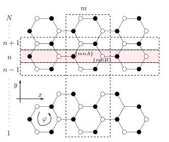
Figure 8: The strip geometry used for our finite-size computations. The strip is $N$ cells wide with arm chair edges and has periodic (open) boundary conditions in the longitudinal (transverse) directions. Each unit cell is labeled by two indices $m$ and $n$, and contains two sites belonging to the $A$ or $B$ sublattices. The phase $\varphi$ of the Haldane model is taken as positive for anticlockwise next to nearest neighbor hopping.

We define the longitudinal current $\hat{J}_{n}^{x}$ as the total current flowing along the $n$-th row of the strip where $n\in 1,\dots,N$, as shown by the shaded area in Fig. 8. Exploiting the periodic boundary conditions along the strip, $\hat{J}_{n}^{x}=\sum_{k_{x}}\hat{J}_{n}(k_{x})$. As shown in Fig. 9, the terms in this summation appear with both positive and negative signs. In particular, the edge currents, $\langle\hat{J}_{1}^{x}\rangle$ and $\langle\hat{J}_{N}^{x}\rangle$, receive opposite contributions which perfectly cancel when $\varphi=\pi/2$.

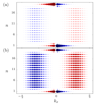
Figure 9: Momentum space contributions to the equilibrium currents along the strip, $\langle\hat{J}_{n}^{x}(k_{x})\rangle$, with $N=20$, $t_{1}=1$, $t_{2}=1/3$ and $M=0$. For clarity, the size of the dots is proportional to the fourth power of $\langle\hat{J}_{n}^{x}(k_{x})\rangle$ and the blue (red) dots indicate negative (positive) values. (a) $\varphi=\pi/3$ showing counter-propagating contributions to the currents. The net currents vanish in the bulk but are non-zero close to the edges; see Fig. 4(a). (b) $\varphi=\pi/2$ showing balanced contributions throughout the strip, leading to $\langle\hat{J}_{n}^{x}\rangle=0$.

Doping the system with particles or holes breaks this symmetry and restores the $2\pi$-periodicity, as shown in Fig. 10.

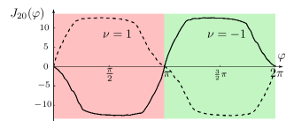
Figure 10: Equilibrium edge current $J_{N}^{x}$ for $N=20$, $t_{1}=1$, $t_{2}=1/3$ and $M=0$ with a $5\%$ particle (solid) or hole (dashed) doping. In contrast to the half-filled case shown in Fig. 4(b), the currents no longer vanish at $\varphi=\pi/2$. Instead, the currents have the same periodicity as the Hamiltonian. The increase or decrease of the edge current at $\varphi=\pi/2$ reflects both the sign of the doping and the Chern index.

The effect of doping is to change the relative contributions of the bulk and the edge states to the total edge currents; for particle (hole) doping the edge (bulk) states contribute more to the overall edge current.

Zeros of the orbital magnetization also occur within the topological phases. As shown in Fig. 11, ${\bm{\mathcal{M}}}(M,\varphi)$ has extrema at $M=0$ and on the boundaries of the topological phases at $M=\pm\sqrt{3}\sin\varphi$. Numerically we observe that the zeros of ${\bm{\mathcal{M}}}$ occur on the sinusoidal loci $M=\pm\sin\varphi$.

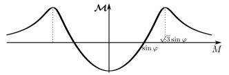
Figure 11: Orbital magnetization $\bm{\mathcal{M}}$ with $N=20$, $t_{1}=1$, $t_{2}=1/3$ and $\varphi=\pi/3$. Numerically we observe that $\bm{\mathcal{M}}$ vanishes within the topological phases when $M=\pm\sin\varphi$. We also observe that $\bm{\mathcal{M}}$ has extrema for $M=0$ and $M=\pm\sqrt{3}\sin\varphi$; the latter correspond to the boundaries of the topological phases as indicated by the dotted lines.

Once again, the effect of doping is to change the relative contributions of the bulk and the edge states to the orbital magnetization; for particle (hole) doping the edge (bulk) states contribute more to $\bm{\mathcal{M}}$.

Dynamics of the Edge Currents.— Following a quantum quench, we observe that the edge currents relax to new values that are comparable to the ground expectation values evaluated for the final Hamiltonian. In these examples we necessarily see finite-size effects due to the finite width of the strip. At late times, we see resurgent oscillations due to the light-cone propagation of currents into the interior of the sample; see Fig. 12.

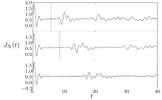
Figure 12: Time dependence of the edge current $J_{N}^{x}(t)$ after a quantum quench from the topological phase with $M=1.4$ to the non-topological phase with $M=1.6$, keeping $t_{1}=1$, $t_{2}=1/3$ and $\varphi=\pi/3$ fixed. This corresponds to the main panel of Fig. 5 over a longer time duration. The three panels from the top to the bottom correspond to strips of width $N=20$, $30$ and $40$ respectively. The appearance of resurgent oscillations is evident in all three panels due to the finite width of our system. The dashed lines indicate the time-scale $t=(N/2)\sqrt{3}/2c$ at which signals propagating from the two edges meet, corresponding to the onset of finite-size effects. The horizontal line corresponds to the ground-state expectation value of the edge current for the post quench Hamiltonian.

The onset timescale for these resurgent oscillations increases with the width of the strip. This timescale is given by $t=d/2c$ where $d=N\sqrt{3}/2$ is the width of the sample and $c=3t_{1}/2\hbar$ is the effective speed of light. This timescale is indicated by the dashed lines in Fig. 12. In order to avoid finite-size effects in our predictions we therefore restrict the domain of our simulations to be within this time interval. The agreement between the results for $N=30$ and $N=40$ in Fig. 5 of the main text highlights that we are probing the intrinsic dynamics of the edge currents, before finite-size effects play a role.

For completeness, in Fig. 13 we show quenches to the topological phase. Numerically we observe that the edge currents approach new values that are very close to those evaluated in the ground state of the final Hamiltonian. Likewise, the oscillation frequencies coincide for quenches to the same final Hamiltonian.

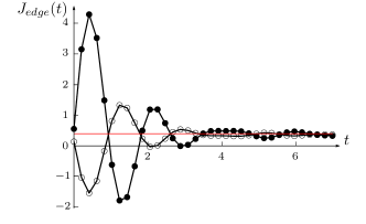
Figure 13: Edge current $J_{N}^{x}(t)$ following a quantum quench within the topological phase (filled circles) and from the non-topological phase to the topological phase (empty circles). We set $N=30$, $t_{1}=1$, $t_{2}=1/3$ and $\varphi=\pi/3$ and consider quenches of the mass parameter $M=0.5\rightarrow 1.4$ (full circles) and $M=2.2\rightarrow 1.4$ (empty circles). The horizontal line corresponds to the ground-state expectation value of the edge current for the post quench Hamiltonian. The coincidence between the oscillation frequencies is consistent with the fact that we quench to the same final Hamiltonian.