Some Exact Properties of the Nonequilibrium Response Function for Transient Photoabsorption

Abstract

The physical interpretation of time-resolved photoabsorption experiments is not as straightforward as for the more conventional photoabsorption experiments conducted on equilibrium systems. In fact, the relation between the transient photoabsorption spectrum and the properties of the examined sample can be rather intricate since the former is a complicated functional of both the driving pump and the feeble probe fields. In this work we critically review the derivation of the time-resolved photoabsorption spectrum in terms of the nonequilibrium dipole response function $\chi$ and assess its domain of validity. We then analyze $\chi$ in detail and discuss a few exact properties useful to interpret the transient spectrum during (overlapping regime) and after (nonoverlapping regime) the action of the pump. The nonoverlapping regime is the simplest to address. The absorption energies are indeed independent of the delay between the pump and probe pulses and hence the transient spectrum can change only by a rearrangement of the spectral weights. We give a close expression of these spectral weights in two limiting cases (ultrashort and everlasting monochromatic probes) and highlight their strong dependence on coherence and probe-envelope. In the overlapping regime we obtain a Lehmann-like representation of $\chi$ in terms of light-dressed states and provide a unifying framework of various well known effects in pump-driven systems. We also show the emergence of spectral sub-structures due to the finite duration of the pump pulse.

I Introduction

Filming a “movie” with electrons and nuclei as actors may sound fantasy-like, but it is de facto a common practice in physics and chemistry modern laboratories. With the impressive march of advances in laser technology, ultrashort (down to the sub-fs time-scale), intense ($\gtrsim 10^{15}$ W/cm²) and focussed pulses of designable shape, hereafter named pumps, are available to move electrons in real or energy space. By recording the photoemission or photoabsorption spectrum produced by a second, weak pulse, hereafter named probe, impacting the sample with a tunable delay from the pump a large variety of ultrafast physical and chemical processes can be documented.Krausz and Ivanov (2009); Berera et al. (2009); Gallmann et al. (2012); Sansone et al. (2012); Gallmann et al. (2013); Kuleff and Cederbaum (2014) Time-resolved pump-and-probe (P&P) spectroscopies have revealed the formation and dynamics of excitons,Kaindl et al. (2003); Wang et al. (2005); Koch et al. (2006); Piris et al. (2009); Cowan et al. (2012) charge-transfer excitations,may ; Asbury et al. (2000); Schnadt et al. (2002); Föhlisch et al. (2005); Gray and Winkler (2005); Remacle and Levine (2006); Rozzi et al. (2013); Falke et al. (2014); pdr auto-ionized statesPfeiffer et al. (2011); Bernhardt et al. (2014a) and light-dressed states,Buth et al. (2007); Glover et al. (2010); Gilbertson et al. (2010); Ranitovic et al. (2011); Tarana and Greene (2012); Lin et al. (2012); Chen et al. (2012a); Chini et al. (2012); Chen et al. (2013a, b); Herrmanna et al. (2013); Chini et al. (2013); Pfeiffer et al. (2013); Wang et al. (2013); Bernhardt et al. (2014b) the evolution of Fano resonances,Wickenhauser et al. (2005); Zhao and Lein (2012); Chu and Lin (2013); Ott et al. (2013, 2014); Argenti et al. (2014) the screening build-up of charged excitations,Huber et al. (2001); Hase et al. (2003); Borisov et al. (2004); Moskalenko et al. (2012) the transient transparency of solids,Srivastava et al. (2004); Nagler and et al. (2009) the motion of valence electrons,Drescher et al. (2002); Niikura et al. (2005); Smirnova et al. (2009); Smirnovaa et al. (2009); Goulielmakis et al. (2010); Pabst et al. (2011) the band-gap renormalization of excited semiconductors,Breusing et al. (2009); Schultze et al. (2013, 2014) how chemical bonds breakZewail (2000); Chen (2005); Sansone et al. (2010); Lawrence and Skinner (2003) and other fundamental phenomena.

A suited P&P spectroscopy to investigate charge-neutral excitations is the time-resolved (TR) photoabsorbtion (PA) spectroscopy.Cavalieri et al. (2007); Wang et al. (2010); Holler et al. (2011) It is well established that PA spectra of equilibrium systems are proportional to the dipole-dipole response function $\chi$,bas ; Strinati (1988); vig ; svl an extremely useful quantity to understand and interpret the experimental results. In pump-driven systems the derivation of a mathematical quantity to interpret TR-PA spectra is slightly more delicate and, in fact, several recent works have been devoted to this subject.Gaarde et al. (2011); Santra et al. (2011); Chu and Lin (2012a); Baggesen et al. (2012); Dutoi et al. (2013) The difficulty in constructing a solid and general TR-PA spectroscopy framework (valid for general P&P envelops, durations and delays and for samples of any thickness) stems from the fact that the probed systems evolve in a strong time-dependent electromagnetic (em) field and hence (i) low-order perturbation theory in the pump intensity may not be sufficiently accurate and (ii) separating the total energy per unit frequency absorbed by the system into a pump and probe contribution is questionable. Furthermore, due to the lack of time-translational invariance the TR-PA spectrum is not an intrinsic property of the pump-driven system, depending it on the shape of the probe field too.

We can distinguish two different approaches to derive a TR-PA formula: the energy approach,Gaarde et al. (2011); Chu and Lin (2012a); Dutoi et al. (2013) which aims at calculating the energy absorbed from only the probe, and the Maxwell approach,Santra et al. (2011); Baggesen et al. (2012); muk which aims at calculating the transmitted probe field (these approaches are equivalent for optically thin and equilibrium samples). We carefully revisit the energy approach, highlight its limitations and infer that it is not suited to perform a spectral decomposition of the absorbed energy. We also re-examine the Maxwell approach and provide a derivation of the TR-PA spectrum in non-magnetic systems without the need of frequently made assumptions like, e.g., slowly-varying probe envelops or ultrathin samples. The final result is that the TR-PA spectrum can be calculated from the single and double convolution of the nonequilibrium response function $\chi$ with the probe field.

For the physical interpretation of TR-PA spectral features a Lehmann-like representation of the nonequilibrium $\chi$ would be highly valuable, as it is in PA spectroscopy of equilibrium systems. In this work we discuss some exact properties of the nonequilibrium $\chi$ and of its convolution with the probe field. When the probe acts after the pump (nonoverlapping regime) $\chi$ can be written as the average over a nonstationary state of the dipole operator-correlator evolving with the equilibrium Hamiltonian of the sample. In this regime the TR-PA spectrum is nonvanishing when the frequency matches the difference of two excited-state energies. As these energies are independent of the delay $\tau$ between the pump and probe field, only the spectral weights can change with $\tau$ (not the absorption regions).psm We discuss in detail how the spectral weights are affected by the coherence between nondegenerate excitations and by the shape of the probe field. A close expression is given in the two limiting cases of ultrashort and everlasting monochromatic probes.

The overlapping regime is, in general, much more complicated to address. The absorption energies cease to be an intrinsic property of the unperturbed system and acquire a dependence on the delay. Nevertheless, an analytic treatment is still possible in some relevant situations. For many-cycle pump fields of duration longer than the typical dipole relaxation time, we show that a Lehmann-like representation of the nonequilibrium $\chi$ in terms of light-dressed states can be used to interpret the TR-PA spectrum. We provide a unifying framework of well known effects in pump-driven systems like, e.g., the AC Stark shift, the Autler-Townes splitting and the Mollow triplet. More analytic results can be found for samples described by a few level systems. In this case, from the exact solution of the nonequilibrium response function with pump fields of finite duration we obtain the dipole moment induced by ultrashort probe fields. The analytic expression shows that (i) the $\tau$-dependent renormalization of the absorption energies follows closely the pump envelope and (ii) a spectral sub-structure characterized by extra absorption energies emerges.

The paper is organized as follows. In Section II we briefly review the principles of TR-PA spectroscopy measurements. We critically discuss the energy approach to PA spectroscopy in equilibrium systems and highlight the limitations which hinder a generalization to nonequilibrium situations. The conceptual problems of the energy approach are overcome by the Maxwell approach which is re-examined and used to derive the transmitted probe field emerging from non-magnetic samples of arbitrary thickness, without any assumption on the shape of the incident pulse. The nonequilibrium dipole-dipole response function $\chi$ is introduced in Section III and related to the transmitted probe field. We analyze $\chi$ in the nonoverlapping regime in Section IV and in the overlapping regime in Section V. Finally, a class of exact solutions in few-level systems for overlapping pump and probe fields is presented in Section VI. Summary and conclusions are drawn in Section VII.

II Time-Resolved Photoabsorption Spectroscopy

In this section we briefly revisit the principles of PA for systems in equilibrium, and subsequently generalize the discussion to the more recent TR-PA for systems driven away from equilibrium. The aim of this preliminary section is to highlight the underlying assumptions of orthodox equilibrium PA theories, identify the new physical ingredients that a nonequilibrium PA theory should incorporate, and eventually obtain a formula for the TR spectrum which is a functional of both the pump and probe fields. Except for a critical review of the literature no original results are present in this section.

II.1 Experimental measurement

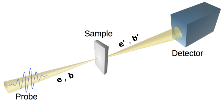
Figure 1: (Color online) Illustration of a PA experiment.

Consider a system in equilibrium and irradiate it with some feeble light (perturbative probe). In Fig. 1 we show a snapshot at time $t$ of a typical equilibrium PA experiment. The incident light is described by the electric and magnetic fields ${\mathbf{e}}(t)$ and ${\mathbf{b}}(t)$ (left side of the sample) whereas the transmitted light is described by the em fields ${\mathbf{e}}^{\prime}(t)$, ${\mathbf{b}}^{\prime}(t)$ (right side of the sample). The experiment measures the total transmitted energy $E^{\prime}$. This quantity is given by the energy flow (or equivalently the Poynting vector) integrated over time (the duration of the experiment) and surface. Denoting by $\mathcal{S}$ the cross section of the incident beam we have (here and in the following integrals with no upper and lower limits go from $-\infty$ to $+\infty$)

$$E^{\prime}=\mbox{$\mathcal{S}$}\frac{c}{4\pi}\int dt\left|{\mathbf{e}}^{\prime}(t)\times{\mathbf{b}}^{\prime}(t)\right|.$$ (1)

The integral in Eq. (1) is finite since the em fields used in an experiment vanish outside a certain time interval. In vacuum the electric and magnetic fields are perpendicular to each other and their cross product is parallel to the direction of propagation. Taking into account that $|{\mathbf{b}}^{\prime}|=|{\mathbf{e}}^{\prime}|$ the transmitted energy in Eq. (1) simplifies to

$$E^{\prime}=\mbox{$\mathcal{S}$}\frac{c}{4\pi}\int dt\left|{\mathbf{e}}^{\prime}(t)\right|^{2}.$$ (2)

From Eq. (2) we see that the transmitted energy $E^{\prime}$ depends on the temporal shape of the electric field. This dependence can be exploited to extract the energy of the neutral excitations of the sample. A typical, systematic way of varying the temporal shape consists in probing the sample with monochromatic light of varying frequency. Taking into account that the electric field is real, its Fourier transform reads

$${\mathbf{e}}^{\prime}(t)=\int_{0}^{\infty}\frac{d\omega}{2\pi}\,\tilde{{\mathbf{e}}}^{\prime}(\omega)e^{-i\omega t}+c.c.$$ (3)

where $c.c$ stands for “complex conjugate”. Unless otherwise defined, quantities with the tilde symbol on top denote the Fourier transform of the corresponding time-dependent quantities. Inserting Eq. (3) back into Eq. (2) we find

$$E^{\prime}=\mbox{$\mathcal{S}$}\frac{c}{2\pi}\int_{0}^{\infty}\frac{d\omega}{2\pi}\left|\tilde{{\mathbf{e}}}^{\prime}(\omega)\right|^{2}.$$ (4)

For monochromatic light of frequency $\omega_{0}$ (in the time interval of the experiment) the transmitted field $\tilde{{\mathbf{e}}}^{\prime}(\omega)$ is peaked at $\omega\simeq\omega_{0}$ and hence $E^{\prime}\simeq\mbox{$\mathcal{S}$}\frac{c}{2\pi}\frac{\Delta\omega}{2\pi}\left|\tilde{{\mathbf{e}}}^{\prime}(\omega_{0})\right|^{2}$, where $\Delta\omega$ is the width of the peaked function $\tilde{{\mathbf{e}}}^{\prime}(\omega)$. Therefore the quantity

$$\tilde{W}^{\prime}(\omega)\equiv\mbox{$\mathcal{S}$}\frac{c}{2\pi}\left|\tilde{{\mathbf{e}}}^{\prime}(\omega)\right|^{2}\quad,\quad\omega>0$$ (5)

can be interpreted as the transmitted energy per unit frequency.

Alternatively $\tilde{W}^{\prime}(\omega)$ could be measured using fields of arbitrary temporal shape and a spectrometer. As this is also the technique in TR-PA experiments, and the method to elaborate the data of the real-time simulations of Section VI is based on this technique, we shortly describe its principles. The spectrometer, placed between the sample and the detector, splits the transmitted beam into two halves and generates a tunable delay $\delta$ for one of the halves. The resulting electric field at the detector is therefore $\frac{1}{2}\left({\mathbf{e}}^{\prime}(t)+{\mathbf{e}}^{\prime}(t-\delta)\right)$, and the measured transmitted energy is

$$E^{\prime}(\delta)=\mbox{$\mathcal{S}$}\frac{c}{4\pi}\int dt\left|\frac{{\mathbf{e}}^{\prime}(t)+{\mathbf{e}}^{\prime}(t-\delta)}{2}\right|^{2}.$$ (6)

The PA experiment is repeated for different delays $\delta$, and the results are collected to perform a cosine transform

$$\tilde{E}^{\prime}(\nu)\equiv\int d\delta\;E^{\prime}(\delta)\cos(\nu\delta).$$ (7)

The relation between $\tilde{E}^{\prime}$ and $\tilde{W}^{\prime}$ is readily found. Using Eq. (3) we get

$$E^{\prime}(\delta)=\mbox{$\mathcal{S}$}\frac{c}{2\pi}\int_{0}^{\infty}\frac{d\omega}{2\pi}\left|\tilde{{\mathbf{e}}}^{\prime}(\omega)\right|^{2}\frac{1+\cos(\omega\delta)}{2}.$$ (8)

Inserting this result into Eq. (7) and taking into account the identity $\int d\delta\cos(\omega\delta)\cos(\nu\delta)=\pi\left[\delta(\omega+\nu)+\delta(\omega-\nu)\right]$ we find $\tilde{E}^{\prime}(\nu)=\pi\delta(\nu)E^{\prime}+\mbox{$\mathcal{S}$}\frac{c}{8\pi}\left|\tilde{{\mathbf{e}}}^{\prime}(\nu)\right|^{2}.$ Thus for every $\nu\neq 0$ we have $\tilde{W}^{\prime}(\nu)=4\tilde{E}^{\prime}(\nu)$.

The PA experiment can be repeated without the sample to measure the energy per unit frequency $\tilde{W}(\omega)$ of the incident beam. The difference

$$\tilde{S}(\omega)=\tilde{W}(\omega)-\tilde{W}^{\prime}(\omega)>0$$ (9)

is therefore the missing energy per unit frequency. How to relate this experimental quantity to the excited energies and excited states of the sample is well established and will be reviewed in the next Section.

The main novelty introduced by TR-PA experiments consists in probing the sample in a nonstationary (possibly driven) state. The sample is driven out of equilibrium by an intense laser pulse described by the em fields ${\mathbf{E}}(t)$ and ${\mathbf{B}}(t)$, and subsequently probed with the em fields ${\mathbf{e}}(t)$ and ${\mathbf{b}}(t)$, see Fig. 2. We refer to ${\mathbf{E}}(t)$ and ${\mathbf{B}}(t)$ as the pump fields. To extract information on the missing probe energy the transmitted pump field is not measured, see again Fig. 2. As the sample is not in its ground state the transmitted beam is also made of photons produced by the stimulated emission. These photons have the same frequency and direction of the probe photons and, therefore, the inequality in Eq. (9) is no longer guaranteed.

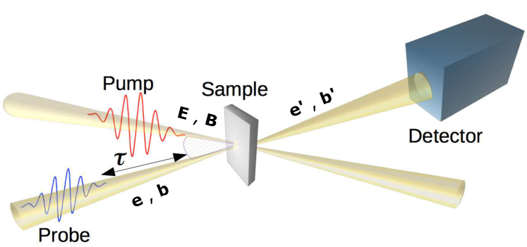
Figure 2: (Color online) Illustration of a TR-PA experiment.

II.2 Energy approach: PA in equilibrium

In this section we obtain an expression for the spectrum $\tilde{S}(\omega)$ of systems initially in equilibrium in their ground state (the finite-temperature generalization is straightforward). We use an approach based on the energy dissipated by the sample and highlight those parts in the derivation where the hypothesis of initial equilibrium and weak em field is used. We advance that this approach cannot be generalized to nonequilibrium situations.

For a system driven out of equilibrium by an external (transverse) electric field ${\mathbf{E}}_{\rm ext}$ the energy absorbed per unit time, i.e., the power dissipated by the system, is

$$\mbox{$\mathcal{P}$}(t)=-\int d{\mathbf{r}}\;{\mathbf{J}}({\mathbf{r}}t)\cdot{\mathbf{E}}_{\rm ext}({\mathbf{r}}t),$$ (10)

where ${\mathbf{J}}$ is the current density and $e=-1$ is the electric charge. This well-known formula is valid only provided that the electric field generated by the induced current ${\mathbf{J}}$ is much smaller than ${\mathbf{E}}_{\rm ext}$. For the time being let us assume that this is the case. We also assume that the probed systems are nanoscale samples like atoms and molecules or thin slabs of solids. Then the wavelength of the incident em field is typically much larger than the longitudinal dimension of the sample and the spatial dependence of ${\mathbf{E}}_{\rm ext}$ can be ignored. Writing ${\mathbf{J}}=\mbox{\boldmath$\nabla$}({\mathbf{r}}\cdot{\mathbf{J}})-(\mbox{\boldmath$\nabla$}\cdot{\mathbf{J}}){\mathbf{r}}$, discarding the total divergence and using the continuity equation the power becomes

$$\mbox{$\mathcal{P}$}(t)=-\int d{\mathbf{r}}\;\frac{\partial n({\mathbf{r}}t)}{\partial t}{\mathbf{r}}\cdot{\mathbf{E}}_{\rm ext}(t),$$ (11)

where $n$ is the electron density. The integral of the power between any two times $t_{1}$ and $t_{2}$ yields the difference between the energy of the system at time $t_{2}$ and the energy of the system at time $t_{1}$:

$$E_{\rm sys}(t_{2})-E_{\rm sys}(t_{1})=-\int_{t_{1}}^{t_{2}}dt\;{\mathbf{E}}_{\rm ext}(t)\cdot\frac{d}{dt}{\mathbf{d}}(t),$$ (12)

where we found convenient to define the dipole moment

$${\mathbf{d}}(t)=\int d{\mathbf{r}}\;{\mathbf{r}}\,n({\mathbf{r}}t).$$ (13)

We observe that nowhere the assumption of small external em fields and/or the assumption of a system in equilibrium are made in the derivation of Eq. (12). It is also important to emphasize the semiclassical nature of Eq. (12). Suppose that the sample is initially in its ground state with energy $E_{g}$. We switch the em field on at a time $t=t_{\rm on}$ and switch it off at a time $t=t_{\rm off}$. According to Eq. (12) the difference $E_{\rm sys}(t)-E_{g}$ remains constant for any $t>t_{\rm off}$. Physically, however, this is not what happens. At times $t\gg t_{\rm off}$ the sample is back in its ground state since there has been enough time to relax (via the spontaneous emission of light). Hence the correct physical result should be $E_{\rm sys}(t\to\infty)-E_{g}=0$. In Eq. (12) the description of the em field is purely classical and does not capture the phenomenon of spontaneous emission. Nevertheless, a spontaneous emission process occurs on a time scale much longer than the duration of a typical PA experiment. The semiclassical formula is therefore accurate for times $t\gtrsim t_{\rm off}$ and, consequently, the quantity

$$E_{\rm abs}=-\int dt\;{\mathbf{E}}_{\rm ext}(t)\cdot\frac{d}{dt}{\mathbf{d}}(t)$$ (14)

can be identified with the increase in the energy of the sample just after the em field has been switched off. We refer to $E_{\rm abs}$ as the absorbed energy. Let us see how to relate Eq. (14) to the missing energy $\tilde{S}(\omega)$ measured in an experiment.

In equilibrium PA experiments ${\mathbf{E}}_{\rm ext}={\mathbf{e}}$ is the probing field discussed in Section II.1. Let $E=\int\frac{d\omega}{2\pi}\tilde{W}(\omega)$ and $E^{\prime}=\int\frac{d\omega}{2\pi}\tilde{W}^{\prime}(\omega)$ be the total energy of the incident and transmitted beam respectively. Then the difference $E-E^{\prime}$ is the energy transferred to the sample, i.e., the absorbed energy of Eq. (14)

$$E-E^{\prime}=E_{\rm abs}.$$ (15)

We write the dipole moment ${\mathbf{d}}={\mathbf{d}}_{\rm eq}+{\mathbf{d}}_{p}$ as the the sum of the equilibrium value ${\mathbf{d}}_{{\rm eq}}$ and the probe induced variation ${\mathbf{d}}_{p}$. Since ${\mathbf{d}}_{{\rm eq}}$ is constant in time the absorbed energy in frequency space reads

$$E_{\rm abs}=i\int_{0}^{\infty}\frac{d\omega}{2\pi}\omega\;\tilde{{\mathbf{e}}}^{\ast}(\omega)\cdot\tilde{{\mathbf{d}}}_{p}(\omega)+c.c.$$ (16)

Taking into account Eq. (15) and the definition of $\tilde{S}$ in Eq. (9) we also have

$$E_{\rm abs}=\int\frac{d\omega}{2\pi}\tilde{S}(\omega).$$ (17)

We now show that the r.h.s. of Eqs. (16) and (17) are the same because the integrands are the same. The transmitted em field $\tilde{{\mathbf{e}}}^{\prime}(\omega)$ at frequency $\omega$ depends, to lowest order in ${\mathbf{e}}$, only on $\tilde{{\mathbf{e}}}(\omega)$ at the same frequency $\omega$ since the system is initially in equilibrium (hence invariant under time translations). This implies that if the probe field has $N$ frequencies $\omega_{1},\ldots,\omega_{N}$ then the total missing energy $E-E^{\prime}$ is the sum of the missing energies of $N$ independent PA experiments carried out with monochromatic beams of frequencies $\omega_{1},\ldots,\omega_{N}$. The same is true for the energy absorbed by the sample: $\tilde{{\mathbf{d}}}_{p}(\omega)$ depends only on $\tilde{{\mathbf{e}}}(\omega)$ since the probe-induced dipole moment is linear in ${\mathbf{e}}$. Therefore for systems in equilibrium and to lowest order in the probing fields we can write

$$\tilde{S}(\omega)=i\omega\;\tilde{{\mathbf{e}}}^{\ast}(\omega)\cdot\tilde{{\mathbf{d}}}_{p}(\omega)+c.c.$$ (18)

The approaches to calculate the right hand side of Eq. (18) can be grouped into two classes. In one (recently emerging) class one perturbs the system with an em field ${\mathbf{e}}(t)$, calculates the time-dependent dipole moment either by solving the Schrödinger/Liouville equation or by using other methods,Bertsch et al. (2000); Sun et al. (2007); Kwong and Bonitz (2000); Dahlen and van Leeuwen (2007); von Friesen et al. (2009); Attaccalite et al. (2011); Myöhänen et al. (2012); Latini et al. (2014); De Giovannini et al. (2013); Neidel et al. (2013); Crawford-Uranga et al. (2014) and then Fourier transforms it. The other (more traditional) class avoids time-propagations and works directly in frequency space. To lowest order in ${\mathbf{e}}$ the Kubo formula gives

$$d_{p,i}(t)=\sum_{j}\int dt^{\prime}\chi_{ij}(t,t^{\prime})e_{j}(t^{\prime})$$ (19)

where $\chi$ is the (retarded) dipole-dipole response function. For a system with Hamiltonian $\hat{H}$ in the ground state $|\Psi_{g}\rangle$ of energy $E_{g}$ we have

$$i\chi_{ij}(t,t^{\prime})\! = \!\theta(t-t^{\prime})\langle\Psi_{g}|e^{i\hat{H}t}\hat{d}_{i}e^{-i\hat{H}(t-t^{\prime})}\hat{d}_{j}e^{-i\hat{H}t^{\prime}}-{\rm H.c.}|\Psi_{g}\rangle$$ (20)

$$= \!\theta(t-t^{\prime})\langle\Psi_{g}|\hat{d}_{i}e^{-i(\hat{H}-E_{g})(t-t^{\prime})}\hat{d}_{j}-{\rm H.c.}|\Psi_{g}\rangle$$

where H.c. stands for “hermitian conjugate” and $\hat{d}_{i}$ is the $i$-th component of the dipole-moment operator. As expected the equilibrium response function $\chi$ depends on the time-difference only. Fourier transforming Eq. (19) and inserting the result into Eq. (18) we get

$$\tilde{S}(\omega)=\omega\sum_{ij}\tilde{e}^{\ast}_{i}(\omega)\mbox{$\mathcal{L}$}_{ij}(\omega)\tilde{e}_{j}(\omega),$$ (21)

with $\mbox{$\mathcal{L}$}_{ij}(\omega)\equiv i\left[\tilde{\chi}_{ij}(\omega)-\tilde{\chi}_{ji}^{\ast}(\omega)\right]$. The response function $\tilde{\chi}(\omega)$ can be calculated by several means without performing a time propagation. From the Lehmann representation of $\chi$ it is easy to verify that $\mathcal{L}$ is positive semidefinite for positive frequencies and negative semidefinite otherwise. Consequently $\tilde{S}$ is manifestly positive, in agreement with Eq. (9).

II.3 Energy approach: PA out of equilibrium

In a typical TR-PA experiment both the pump and probe fields are very short (fs-as) laser pulses with a delay $\tau$ between them. If $\tau<0$ then the probe acts before the pump and we recover the PA spectra of equilibrium systems. On the other hand if $\tau>0$ then $\tilde{S}(\omega)$ acquires a dependence on $\tau$. This dependence can be used to follow the evolution of the system in real time. However, for the physical interpretation of what we are actually following it is necessary to generalize the equilibrium PA theory to nonequilibrium situations.

Let the external electric field ${\mathbf{E}}_{\rm ext}$ be the sum of the pump field ${\mathbf{E}}$ and probe field ${\mathbf{e}}$, i.e., ${\mathbf{E}}_{\rm ext}={\mathbf{E}}+{\mathbf{e}}$. In this case Eq. (14) yields the total energy absorbed by the system. As the experiment detects only the energy of the transmitted probe field the use of the energy approach for TR-PA is not straightforward. One might argue that the energy absorbed from the probe is given by Eq. (14) in which ${\mathbf{E}}_{\rm ext}\to{\mathbf{e}}$

$$E_{\rm abs}\stackrel{{\scriptstyle?}}{{=}}-\int dt\;{\mathbf{e}}(t)\cdot\frac{d}{dt}{\mathbf{d}}(t).$$ (22)

However, this formula cannot be always correct. Suppose that the pump field is also feeble and can be treated as a small perturbation. Then, the transmitted probe field $\tilde{{\mathbf{e}}}^{\prime}(\omega)$ depends on $\tilde{{\mathbf{E}}}(\omega)+\tilde{{\mathbf{e}}}(\omega)$ (linear response theory). These fields are independent of position inside the sample. In a larger space, like that of the laboratory, they do depend on ${\mathbf{r}}$ and this dependence specifies the direction of propagation. Let $\tilde{{\mathbf{E}}}({\mathbf{K}}\omega)$ and $\tilde{{\mathbf{e}}}({\mathbf{k}}\omega)$ be the spatial Fourier transform of the pump and probe fields. For isotropic systems $\tilde{{\mathbf{e}}}^{\prime}({\mathbf{k}}\omega)$ depends only on $\tilde{{\mathbf{e}}}({\mathbf{k}}\omega)$ since $\tilde{{\mathbf{E}}}({\mathbf{k}}\omega)$ vanishes for ${\mathbf{k}}$ parallel to the direction of propagation of the probe. This implies that the missing energy per unit frequency is independent of the pump, a conclusion which is not in agreement with Eq. (22). In fact, $E_{\rm abs}$ depends on ${\mathbf{E}}$ whenever the pump-induced variation of ${\mathbf{d}}$ is not orthogonal to ${\mathbf{e}}$.

To cure this problem we could write ${\mathbf{d}}={\mathbf{d}}_{P}+{\mathbf{d}}_{p}$, where ${\mathbf{d}}_{P}$ is the value of the dipole moment when only the pump field is present whereas ${\mathbf{d}}_{p}$ is the probe-induced variation, and say that the missing probe energy is

$$E_{\rm abs}\stackrel{{\scriptstyle?}}{{=}}-\int dt\;{\mathbf{e}}(t)\cdot\frac{d}{dt}{\mathbf{d}}_{p}(t).$$ (23)

This expression is by construction correct for perturbative pumps. For pumps of arbitrary strength Eq. (23) cannot be proved or disproved using exclusively energy considerations. For the sake of the argument, however, let us assume that Eq. (23) is the correct missing energy. There is still a conceptual problem to overcome if we are interested in the missing energy per unit frequency. For strong pump fields the sample is in a nonstationary state and hence the transmitted probe field $\tilde{{\mathbf{e}}}^{\prime}(\omega)$ depends on the entire function $\tilde{{\mathbf{e}}}$, not only on the value $\tilde{{\mathbf{e}}}(\omega)$ at the same frequency. Thus the reasoning made below Eq. (17) does not apply. In particular if ${\mathbf{e}}$ is monochromatic then ${\mathbf{e}}^{\prime}$ (as well as ${\mathbf{d}}_{p}$) is, in general, not monochromatic. Consequently $\tilde{S}\propto|\tilde{{\mathbf{e}}}|^{2}-|\tilde{{\mathbf{e}}}^{\prime}|^{2}$ is, in general, not monochromatic either. If we used the formula in Eq. (18) we would instead find that $\tilde{S}$ is peaked at only one frequency since $\tilde{{\mathbf{e}}}$ is peaked at only one frequency. To overcome these problems one has to abandon the energy approach and calculate explicitly the transmitted probe field.

II.4 Maxwell approach

To overcome the difficulties of the energy approach we use the Maxwell equations to calculate explicitly the transmitted probe field. In a nonmagnetic medium the total electric field $\mathcal{E}$, i.e., the sum of the external and induced field, satisfies the equationmuk ; lou

$$\nabla^{2}\mbox{\boldmath$\mathcal{E}$}-\frac{1}{c^{2}}\frac{\partial^{2}\mbox{\boldmath$\mathcal{E}$}}{\partial t^{2}}=-\frac{4\pi}{c^{2}}\frac{\partial\langle{\mathbf{J}}\rangle}{\partial t},$$ (24)

where $\langle{\mathbf{J}}\rangle({\mathbf{r}}t)$ is the macroscopic current density, i.e., the spatial average of the current density over small volumes around ${\mathbf{r}}$. In the derivation of Eq. (24) one uses that $\mbox{\boldmath$\nabla$}\times\mbox{\boldmath$\nabla$}\times\mbox{\boldmath$\mathcal{E}$}=\mbox{\boldmath$\nabla$}(\mbox{\boldmath$\nabla$}\cdot\mbox{\boldmath$\mathcal{E}$})-\nabla^{2}\mbox{\boldmath$\mathcal{E}$}$ and that $\mbox{\boldmath$\nabla$}\cdot\mbox{\boldmath$\mathcal{E}$}=0$ since the sample is charge neutral (in a macroscopic sense). Let $\hat{{\mathbf{N}}}$ and $\hat{{\mathbf{n}}}$ be the unit vectors along the propagation direction of the pump and probe fields respectively. In TR-PA experiments these vectors are not parallel for otherwise the detector would measure the transmitted pump intensity too. The time-dependence of the macroscopic current density arises when the pump and probe fields interact with the electrons in the sample. For transverse pump and probe fields and for isotropic systems $\langle{\mathbf{J}}\rangle$ is the sum of transverse waves propagating along the directions $QK\hat{{\mathbf{N}}}+qk\hat{{\mathbf{n}}}$ with $Q$ and $q$ integers, and $K$ and $k$ the pump and probe wave numbers respectively. Consequently, the total electric field too is the sum of waves propagating along $QK\hat{{\mathbf{N}}}+qk\hat{{\mathbf{n}}}$, and Eq. (24) can be solved for each direction separately.

We define $\mbox{\boldmath$\mathcal{E}$}_{p}$ and $\langle{\mathbf{J}}\rangle_{p}$ as the wave of the electric field and current density propagating toward the detector (hence $Q=0$ and $q=1$). The vectors $\mbox{\boldmath$\mathcal{E}$}_{p}$ and $\langle{\mathbf{J}}\rangle_{p}$ depend on the spatial position ${\mathbf{r}}$ only through $x=\hat{{\mathbf{n}}}\cdot{\mathbf{r}}$ (transverse fields) and are parallel to some unit vector $\mbox{\boldmath$\varepsilon$}_{p}$ lying on the plane orthogonal to $\hat{{\mathbf{n}}}$ (the generalization to multiple polarization is straightforward, see Section VI.2): $\mbox{\boldmath$\mathcal{E}$}_{p}=\mbox{\boldmath$\varepsilon$}_{p}\mbox{$\mathcal{E}$}_{p}(x\,t)$ and $\langle{\mathbf{J}}\rangle_{p}=\mbox{\boldmath$\varepsilon$}_{p}J_{p}(x\,t)$. Equation (24) implies that

$$\frac{\partial^{2}\mbox{$\mathcal{E}$}_{p}}{\partial x^{2}}-\frac{1}{c^{2}}\frac{\partial^{2}\mbox{$\mathcal{E}$}_{p}}{\partial t^{2}}=-\frac{4\pi}{c^{2}}\frac{\partial J_{p}}{\partial t},$$ (25)

which is a one-dimensional wave equation that can be solved exactly without assuming slowly-varying probe envelopsSantra et al. (2011) or ultrathin samples.Baggesen et al. (2012) The electric field $\mbox{$\mathcal{E}$}_{p}$ is the sum of an arbitrary solution $h(t-x/c)$ of the homogeneous equation and of an arbitrary special solution $s(x\,t)$: $\mbox{$\mathcal{E}$}_{p}(x\,t)=h(t-x/c)+s(x\,t)$. Without loss of generality we take the boundaries of the sample at $x=0$ and $x=L$. Let $e(t-x/c)$ be the amplitude of the incident probe field which at time $t=0$ is localized somewhere on the left of the sample. Imposing the boundary condition $\mbox{$\mathcal{E}$}_{p}(x\,0)=e(-x/c)$ we then obtain

$$\mbox{$\mathcal{E}$}_{p}(x\,t)=e(t-x/c)-s(x-ct\,0)+s(x\,t).$$ (26)

The special solution $s(x\,t)$ is found by inverting the one-dimensional d’Alambertian $\oblong\equiv\frac{\partial^{2}}{\partial x^{2}}-\frac{1}{c^{2}}\frac{\partial^{2}}{\partial t^{2}}$. The Green’s function $G(x\,t)$ solution of $\oblong G(x\,t)=\delta(x)\delta(t)$ is

$$G(x\,t)=-\frac{c}{2}\,\theta(t)\chi_{[-ct,ct]}(x),$$ (27)

where $\chi_{[a,b]}(x)=1$ if $x\in(a,b)$ and zero otherwise. Therefore the special solution reads

$$s(x\,t)=\frac{2\pi}{c}\int_{-\infty}^{t}dt^{\prime}\int_{-x-c(t-t^{\prime})}^{x+c(t-t^{\prime})}dx^{\prime}\,\frac{\partial J_{p}(x^{\prime}t^{\prime})}{\partial t^{\prime}}.$$ (28)

Without any loss of generality we can choose the time $t=0$ as the time before which nor the pump and neither the probe have reached the sample. Then $J_{p}=0$ for $t<0$ and hence $s(x\,0)=0$ for all $x$. We conclude that

$$\mbox{$\mathcal{E}$}_{p}(x\,t)=e(t-x/c)+s(x\,t),$$ (29)

with $s$ given in Eq. (28).

We are interested in the electric field on the right of the sample, i.e., in $x=L$, since this is the detected field. Let us therefore evaluate Eq. (28) in $x=L$. Taking into account that $J_{p}(x^{\prime}t^{\prime})$ is nonvanishing only for $x^{\prime}\in(0,L)$ and $t^{\prime}>0$ we have

$$s(L\,t) = \frac{2\pi}{c}\int_{0}^{t}dt^{\prime}\int_{0}^{L}dx^{\prime}\,\frac{\partial J_{p}(x^{\prime}t^{\prime})}{\partial t^{\prime}}$$ (30)

$$= \frac{2\pi}{\mbox{$\mathcal{S}$}c}\mbox{\boldmath$\varepsilon$}_{p}\cdot\int_{V}d{\mathbf{r}}\,\langle{\mathbf{J}}\rangle_{p}({\mathbf{r}}t),$$

where in the second line we integrated over the volume $V=\mbox{$\mathcal{S}$}L$ of the sample. Using again the identity $\langle{\mathbf{J}}\rangle_{p}=\mbox{\boldmath$\nabla$}({\mathbf{r}}\cdot\langle{\mathbf{J}}\rangle_{p})-{\mathbf{r}}(\mbox{\boldmath$\nabla$}\cdot\langle{\mathbf{J}}\rangle_{p})$ and extending the integral over all space (outside $V$ the current density vanishes) we can rewrite Eq. (30) as $s(L\,t)=-\frac{2\pi}{\mbox{$\mathcal{S}$}c}\mbox{\boldmath$\varepsilon$}_{p}\cdot\int d{\mathbf{r}}\,{\mathbf{r}}\,(\mbox{\boldmath$\nabla$}\cdot\langle{\mathbf{J}}\rangle_{p})$. Substituting this result into Eq (29) and taking into account the continuity equation $\mbox{\boldmath$\nabla$}\cdot\langle{\mathbf{J}}\rangle_{p}=-\partial\langle n\rangle_{p}/\partial t$, where $\langle n\rangle_{p}$ is the macroscopic probe-induced change of the electronic density propagating along $\hat{{\mathbf{n}}}$, we eventually obtain the transmitted electric field

$$\mbox{$\mathcal{E}$}_{p}(L\,t)=e(t)+\frac{2\pi}{\mbox{$\mathcal{S}$}c}\mbox{\boldmath$\varepsilon$}_{p}\cdot\frac{d}{dt}\int d{\mathbf{r}}\,{\mathbf{r}}\,\langle n\rangle_{p}({\mathbf{r}}t),$$ (31)

where we discarded the delay $L/c$ in the first term on the right hand side. The volume integral is the probe-induced dipole moment propagating along $\hat{{\mathbf{n}}}$. In general this is not the same as the full probe-induced dipole moment ${\mathbf{d}}_{p}$ defined above Eq. (23) since, to lowest order in the probe field, ${\mathbf{d}}_{p}$ is the sum of waves propagating along $k\hat{{\mathbf{n}}}+QK\hat{{\mathbf{N}}}$. Although it is reasonable to expect that the wave propagating along $\hat{{\mathbf{n}}}$ (i.e., with $Q=0$) has the largest amplitude, it is important to bear in mind this conceptual difference. In fact, in equilibrium PA experiments ${\mathbf{d}}_{p}$ and $\int d{\mathbf{r}}\,{\mathbf{r}}\,\langle n\rangle_{p}$ are the same due to the absence of the pump. For not introducing too many symbols we redefine ${\mathbf{d}}_{p}\equiv\int d{\mathbf{r}}\,{\mathbf{r}}\,\langle n\rangle_{p}$. Then, by definition, ${\mathbf{d}}_{p}$ is parallel to $\mbox{\boldmath$\varepsilon$}_{p}$ and we can cast Eq. (31) in vector notation as

$${\mathbf{e}}^{\prime}(t)={\mathbf{e}}(t)+\frac{2\pi}{\mbox{$\mathcal{S}$}c}\frac{d}{dt}{\mathbf{d}}_{p}(t).$$ (32)

Equation (32) relates the transmitted probe field to the quantum-mechanical average of the probe-induced dipole moment, and it represents the fundamental bridge between theory and experiment. The result has been derived without assuming that the wavelength of the incident field is much larger than the longitudinal dimension of the sample (for thick samples $\mbox{$\mathcal{E}$}_{p}$ can be substantially different from $e$ and the quantum electron dynamics should be coupled to the Maxwell equations). Equation (32) can be used to calculate the missing energy per unit frequency of pump-driven systems. Noteworthy Eq. (32) is valid for positive and negative delays between pump and probe, as well as for situations in which pump and probe overlap in time or even for more exotic situations in which the pump is entirely contained in the time-window of the probe.

III Nonequilibrium response function

From the definition in Eq. (9) the spectrum of a (equilibrium or nonequilibrium) PA experiment is given by

$$\tilde{S}(\omega)=\mbox{$\mathcal{S}$}\frac{c}{2\pi}\left(|\tilde{{\mathbf{e}}}(\omega)|^{2}-|\tilde{{\mathbf{e}}}^{\prime}(\omega)|^{2}\right).$$ (33)

Since ${\mathbf{e}}=\mbox{\boldmath$\varepsilon$}_{p}e$ and ${\mathbf{d}}_{p}=\mbox{\boldmath$\varepsilon$}_{p}d_{p}$ are both parallel to $\mbox{\boldmath$\varepsilon$}_{p}$, so it is ${\mathbf{e}}^{\prime}=\mbox{\boldmath$\varepsilon$}_{p}e^{\prime}$. Then, the Fourier transform of Eq. (32) yields $\tilde{e}^{\prime}(\omega)=\tilde{e}(\omega)-i\frac{2\pi}{\mbox{$\mathcal{S}$}c}\omega\,\tilde{d}_{p}(\omega)$, and the spectrum in Eq. (33) can be rewritten as

$$\tilde{S}(\omega)=-2{\rm Im}\left(\omega\,\tilde{e}^{\ast}(\omega)\tilde{d}_{p}(\omega)\right)-\frac{2\pi}{\mbox{$\mathcal{S}$}c}\left|\omega\,\tilde{d}_{p}(\omega)\right|^{2}.$$ (34)

At the end of Section II.3 we criticized the energy approach since it predicts a single-peak spectrum for monochromatic probes. Let us analyze Eq. (34) for the same case. For monochromatic probes of frequency $\omega_{0}$ the first term in Eq. (34) vanishes for $\omega\neq\omega_{0}$ whereas the second term is nonvanishing at the same frequencies of the transmitted probe field, see Eq. (32), in agreement with the discussion at the end of Section II.3. The quadratic term in the dipole moment is usually discarded in equilibrium PA calculations since $d_{p}$ and $e$ oscillate at the same frequencies, and typically $|\tilde{e}(\omega)|\gg(2\pi/\mbox{$\mathcal{S}$}c)|\omega\tilde{d}_{p}(\omega)|$. If we discard the last term in Eq. (34) then we recover the spectrum of Eq. (18) of the energy approach.

For the physical interpretation of nonequilibrium PA spectra it is crucial to understand the physics contained in the nonequilibrium dipole-dipole response function. In fact, $d_{p}$ can be calculated from the scalar version of the Kubo formula in Eq. (19), i.e.,not (a)

$$d_{p}(t)=\int dt^{\prime}\chi(t,t^{\prime})\mbox{$\mathcal{E}$}_{p}(t^{\prime}).$$ (35)

Here the scalar dipole-dipole response function $\chi$ is defined according to $\chi=\sum_{ij}\varepsilon_{p,i}\chi_{ij}\varepsilon_{p,j}$ and $\mbox{$\mathcal{E}$}_{p}$ is the total electric field ($\mbox{$\mathcal{E}$}_{p}\simeq e$ if the induced field is small). Unfortunately, for pump-driven systems a Lehmann-like formula for $\chi$ does not exist due to the presence of a strong time-dependent perturbation in the Hamiltonian. By introducing the evolution operator $\hat{\mbox{$\mathcal{U}$}}(t,t^{\prime})$ from $t^{\prime}$ to $t$ of the system without the probe, the nonequilibrium dipole-dipole response function reads

$$i\chi(t,t^{\prime})\! = \!\theta(t-t^{\prime})$$

$$\times \!\langle\Psi_{g}|\hat{\mbox{$\mathcal{U}$}}(t_{0},t)\hat{d}\,\hat{\mbox{$\mathcal{U}$}}(t,t^{\prime})\hat{d}\,\hat{\mbox{$\mathcal{U}$}}(t^{\prime},t_{0})-{\rm H.c.}|\Psi_{g}\rangle$$

where $\hat{d}=\mbox{\boldmath$\varepsilon$}_{p}\cdot\hat{{\mathbf{d}}}$ and $t_{0}$ is any time earlier than the switch-on time of the pump and probe fields. As anticipated the nonequilibrium $\chi$ depends on $t$ and $t^{\prime}$ separately. It is clear from Eq. (LABEL:nerf1) that $\chi$ does not have a simple representation in terms of the many-body eigenstates and eigenenergies of the unperturbed system. It is also easy to verify that Eq. (LABEL:nerf1) agrees with Eq. (20) in the absence of the pump.

As a final remark before presenting some exact properties of $\chi$, we observe that in equilibrium, see Eq. (21), the ratio $\tilde{S}(\omega)/|\tilde{e}(\omega)|^{2}$ is independent of the probe field, i.e., it is an intrinsic property of the sample. This is not true in nonequilibrium, even if we discard the last term in Eq. (34) and approximate $\mbox{$\mathcal{E}$}\simeq e$. The physical interpretation of nonequilibrium PA spectra cannot leave out of consideration the shape and duration of the probe, and the relative delay between pump and probe. In the next sections we discuss two relevant situations for interpreting the outcome of a TR-PA experiment.

IV Nonoverlapping pump and probe

Let us consider the case of a probe pulse acting after the pump pulse. We take the time origin $t=0$ as the switch-on time of the probe. Then the pump acts at some time $t=-\tau<0$. For $t>0$ the probe-induced variation of the dipole moment can be calculated from Eq. (35) with lower integration limit $t^{\prime}=0$. As we only need $\chi$ for $t,t^{\prime}>0$ we have $\hat{\mbox{$\mathcal{U}$}}(t_{0},t)=\hat{\mbox{$\mathcal{U}$}}(t_{0},0)e^{i\hat{H}t}$ and similarly $\hat{\mbox{$\mathcal{U}$}}(t^{\prime},t_{0})=e^{-i\hat{H}t^{\prime}}\hat{\mbox{$\mathcal{U}$}}(0,t_{0})$, with $\hat{H}$ the unpertubed Hamiltonian of the system. Defining $|\Psi\rangle\equiv\hat{\mbox{$\mathcal{U}$}}(0,t_{0})|\Psi_{g}\rangle$ as the quantum state of the system at time $t=0$, the response function in Eq. (LABEL:nerf1) becomes

$$i\chi(t,t^{\prime})=\theta(t-t^{\prime})\langle\Psi|e^{i\hat{H}t}\hat{d}\,e^{-i\hat{H}(t-t^{\prime})}\hat{d}\,e^{-i\hat{H}t^{\prime}}-{\rm H.c.}|\Psi\rangle$$ (37)

which closely resembles the equilibrium response function of Eq. (20). In fact, without pump fields $|\Psi\rangle=e^{iE_{g}t_{0}}|\Psi_{g}\rangle$ and Eq. (37) reduces to the equilibrium response function. We emphasize that in the presence of pump fields Eq. (37) is valid only for $t,t^{\prime}>0$.

We expand the quantum state $|\Psi\rangle=\sum_{\alpha}c_{\alpha}|\Psi_{\alpha}\rangle$ in terms of the many-body eigenstates $|\Psi_{\alpha}\rangle$ of $\hat{H}$ with eigenenergy $E_{\alpha}$. The coefficients $c_{\alpha}=\bar{c}_{\alpha}e^{-iE_{\alpha}\tau}$ depend on the delay $\tau$ between the pump and the probe, $\bar{c}_{\alpha}$ being the expansion coefficients of the state of the system at the end of the pump. Inserting the expansion in Eq. (37) and using the completeness relation $\sum_{\gamma}|\Psi_{\gamma}\rangle\langle\Psi_{\gamma}|=1$ we find

$$i\chi(t,t^{\prime})=\theta(t-t^{\prime})\sum_{\alpha\beta\gamma}c^{\ast}_{\alpha}c_{\beta}e^{i\Omega_{\alpha\gamma}t}e^{i\Omega_{\gamma\beta}t^{\prime}}d_{\alpha\gamma}d_{\gamma\beta}-c.c.$$ (38)

where we defined the dipole matrix elements $d_{\alpha\gamma}=\langle\Psi_{\alpha}|\hat{d}|\Psi_{\gamma}\rangle$ and the energy differences $\Omega_{\alpha\gamma}=E_{\alpha}-E_{\gamma}$. In the following we use this result to study the outcome of a PA experiment in two limiting cases, i.e., an ultrashort probe and a monochromatic probe.

IV.1 Ultra-short probe

The probe fields used in TR-PA experiments are ultrashort laser pulses. For optically thin samples the em field generated by the probe-induced dipole moment is negligible and does not substantially affect the quantum evolution of the system. Therefore, we can calculate $d_{p}$ from Eq. (35) with $\mbox{$\mathcal{E}$}=e$. For a delta-like probe $e(t)=e_{0}\delta(t)$, hence $\tilde{e}(\omega)=e_{0}$, we find

$$d_{p}(t)=-ie_{0}\sum_{\alpha\beta\gamma}c^{\ast}_{\alpha}c_{\beta}e^{i\Omega_{\alpha\gamma}t}d_{\alpha\gamma}d_{\gamma\beta}+c.c.$$ (39)

where we used the explicit form of the response function in Eq. (38). Fourier transforming this result we obtain the spectrum

$$\tilde{S}(\omega) = -2\omega e_{0}^{2}\sum_{\alpha\beta\gamma}{\rm Im}\big{[}e^{i\Omega_{\alpha\beta}\tau}\,\bar{c}^{\ast}_{\alpha}\bar{c}_{\beta}d_{\alpha\gamma}d_{\gamma\beta}$$ (40)

$$\times \big{(}\frac{1}{\omega-\Omega_{\gamma\alpha}+i\eta}-\frac{1}{\omega+\Omega_{\gamma\beta}+i\eta}\big{)}\big{]}$$

where $\eta$ is a positive infinitesimal and we discarded the quadratic term in $d_{p}$ (thin samples). In Eq. (40) the dependence on the delay $\tau$ enters exclusively through the phase factors and, consequently, it is only responsible for modulating the amplitude of the absorption peaks. The position of the peaks is instead an intrinsic property of the unperturbed system. Thus, a change in the peak-position (discrete spectrum) or in the onset of a continuum (continuum spectrum) due to $\tau$ should not be attributed to a change of the many-body energies but to a redistribution of the spectral weights.

Let us discuss Eq. (40) in some detail. For a system in equilibrium in the ground state (no pump) $c_{\alpha}=1$ for $\alpha=g$ and $c_{\alpha}=0$ otherwise, and the spectrum reduces to

$$\tilde{S}(\omega)=2\pi\omega e_{0}^{2}\sum_{\gamma}|d_{g\gamma}|^{2}\left(\delta(\omega-\Omega_{\gamma g})-\delta(\omega+\Omega_{\gamma g})\right).$$ (41)

Since $E_{\gamma}>E_{g}$ the spectrum is nonnegative, in agreement with Eq. (9). In particular the height of the peak at some frequency $\omega_{0}$ is given by $h_{g}=2\pi|\omega_{0}|e_{0}^{2}\sum_{\gamma:\Omega_{\gamma g}=|\omega_{0}|}|d_{g\gamma}|^{2}\geq 0$. It is also interesting to consider the hypothetical situation of a pump pulse which brings the system from the ground state to an excited state $|\Psi\rangle=|\Psi_{x}\rangle$ with energy $E_{x}$. As the system is stationary this is the simplest example of a nonequilibrium situation. In the stationary case we have $c_{\alpha}=1$ for $\alpha=x$ and $c_{\alpha}=0$ otherwise, and hence the spectrum is again given by Eq. (41) with the only difference that the subscript “$g$” is replaced by the subscript “$x$”. Since $E_{x}$ is not the lowest energy the positivity of the spectrum is no longer guaranteed. In fact, the height of the peak at frequency $\omega_{0}$ is

$$h_{x}=2\pi\omega_{0}e_{0}^{2}\,\big{(}\sum_{\gamma:\Omega_{\gamma x}=\omega_{0}}|d_{x\gamma}|^{2}-\sum_{\gamma:\Omega_{\gamma x}=-\omega_{0}}|d_{x\gamma}|^{2}\big{)}$$ (42)

which can be either positive or negative. The sign is positive if the absorption rate is larger than the rate for stimulated emission and negative otherwise. We observe that in the stationary case the spectrum is independent of the delay.

The most general situation is a system in a nonstationary state. From Eq. (40) the peak intensity at some frequency $\omega_{0}$ reads

$$h=2\pi\omega_{0}e_{0}^{2}\sum_{\alpha\beta}\sum_{\pm}\pm\!\!\sum_{\gamma:\Omega_{\gamma\alpha}=\pm\omega_{0}}{\rm Re}\left[e^{i\Omega_{\alpha\beta}\tau}\,\bar{c}^{\ast}_{\alpha}\bar{c}_{\beta}d_{\alpha\gamma}d_{\gamma\beta}\right],$$ (43)

where we introduced the short-hand notation $\sum_{\pm}A_{\pm}=A_{+}+A_{-}$, with $A$ an arbitrary mathematical expression. If $|\Psi\rangle$ is a superposition of degenerate eigenstates, hence $\bar{c}_{\alpha}\neq 0$ for $E_{\alpha}=E$ and $\bar{c}_{\alpha}=0$ otherwise, then the system is stationary and the height is independent of the delay. The dependence on $\tau$ is manifest only for $|\Psi\rangle$ a superposition of nondegenerate eigenstates. The simplest example is a system in a superposition of two eigenstates with energy $E_{a}$ and $E_{b}$, real coefficients $\bar{c}_{a}$ and $\bar{c}_{b}$ and real dipole matrix elements. In this case Eq. (43) yields $h=h_{a}+h_{b}+h_{ab}\cos(\Omega_{ab}\tau)$ where $h_{x=a,b}$ is defined as in Eq. (42) and

$$h_{ab}=2\pi\omega_{0}e_{0}^{2}\bar{c}_{a}\bar{c}_{b}\sum_{\alpha=a,b}\sum_{\pm}\pm\!\!\sum_{\gamma:\Omega_{\gamma\alpha}=\pm\omega_{0}}d_{a\gamma}d_{b\gamma}.$$

The spectral fingerprint of a nonstationary system is the modulation of the peak intensities with $\tau$. These coherent oscillations have been first observed in Ref. Goulielmakis et al., 2010.

IV.2 Monochromatic probe

The induced electric field of thick samples is not negligible and can last much longer than the external probe pulse. In this case the quantum evolution of the system should be coupled to the Maxwell equations to determine the total field self-consistently.muk ; Ziolkowski et al. (1995); Buth et al. (2007); Gaarde et al. (2011); Chu and Lin (2012b); Chen et al. (2012b); Chu and Lin (2013); Wu et al. (2013a); Pfeiffer et al. (2013); Otobe et al. (2009); Yabana et al. (2012); Wachter et al. (2014); Deinega and Seideman (2014) For a typical sub-as pulse $e(t)$ centered around a resonant frequency $\omega_{0}$ the total electric field $\mbox{$\mathcal{E}$}(t)$ is dominated by oscillations of frequency $\omega_{0}$ decaying over the same time-scale of the induced dipole moment (in atomic gases this time-scale can be as long as hundreds of fs). Let us explore the outcome of a TR-PA experiment for a total field of the form, e.g., $\mbox{$\mathcal{E}$}(t)=\mbox{$\mathcal{E}$}_{0}\theta(t)\sin(\omega_{0}t)$, $\omega_{0}>0$. Taking into account Eq. (38) we find

$$d_{p}(t)=\frac{i}{2}\mbox{$\mathcal{E}$}_{0}\sum_{\alpha\beta\gamma}\sum_{\pm}c^{\ast}_{\alpha}c_{b}d_{\alpha\gamma}d_{\gamma\beta}\frac{e^{i(\Omega_{\alpha\beta}\pm\omega_{0})t}-e^{i\Omega_{\alpha\gamma}t}}{\pm(\Omega_{\gamma\beta}\pm\omega_{0})}+c.c.$$ (44)

If $|\Psi\rangle=|\Psi_{x}\rangle$ (stationary system) then $c_{\alpha}=\delta_{\alpha x}$ and the dominant contributions in Eq. (44) come from eigenstates with energy $E_{\gamma}=E_{x}+\omega_{0}$ in the “$-$” sum and from eigenstates with energy $E_{\gamma}=E_{x}-\omega_{0}$ in the “$+$” sum. Therefore Eq. (44) is well approximated by

$$d_{p}(t)=\mbox{$\mathcal{E}$}_{0}\,t\cos(\omega_{0}t)\sum_{\pm}\pm\sum_{\gamma:\Omega_{\gamma x}=\pm\omega_{0}}|d_{x\gamma}|^{2}.$$ (45)

As expected the dipole moment oscillates at the same frequency of the electric field. Unlike the spectrum of an ultrashort probe, in the monochromatic case $\tilde{S}(\omega)$ has at most one peak. For $x=g$ (ground state) the “$-$” sum vanishes since $\Omega_{\gamma g}>0$, and we recover the well know physical interpretation of equilibrium PA experiments: peaks in $\tilde{S}(\omega)$ occur in correspondence of the energy of a charge neutral excitation. This remains true for $x\neq g$ but the sign of the oscillation amplitude can be either positive or negative. Notice that the oscillation amplitude is proportional to $h_{x}$ in Eq. (42) and it is independent of the delay.

In the nonstationary case $|\Psi\rangle$ is a superposition of nondegenerate eigenstates. For a fixed $\beta$ in Eq. (44) the dominant contributions come from eigenstates with energy $E_{\gamma}=E_{\beta}+\omega_{0}$ in the “$-$” sum and from eigenstates with energy $E_{\gamma}=E_{\beta}-\omega_{0}$ in the “$+$” sum. Writing $\Omega_{\alpha\gamma}=\Omega_{\alpha\beta}+\Omega_{\beta\gamma}$ it is straightforward to show that

$$d_{p}(t) \!\!=\mbox{$\mathcal{E}$}_{0}\frac{t}{2}\sum_{\alpha\beta}\sum_{\pm}\pm\,c^{\ast}_{\alpha}c_{\beta}e^{i\Omega_{\alpha\beta}t}$$ (46)

$$\times \!\!\!\!\!\!\!\big{(}e^{\mp i\omega_{0}t}\!\!\sum_{\gamma:\Omega_{\gamma\beta}=\pm\omega_{0}}d_{\alpha\gamma}d_{\gamma\beta}+e^{\pm i\omega_{0}t}\!\!\sum_{\gamma:\Omega_{\gamma\alpha}=\pm\omega_{0}}d_{\alpha\gamma}d_{\gamma\beta}\big{)}.\quad\quad$$

As anticipated below Eq. (34) $d_{p}(t)$ is not monochromatic in a nonstationary situation, the frequencies of the oscillations being $\omega_{0}\pm\Omega_{\alpha\beta}$. Can these extra frequencies be seen in the TR-PA spectrum? The answer is affirmative since $\tilde{e}(\omega)$ is a broad function centered in $\omega_{0}$ and hence for $|\Omega_{\alpha\beta}|$ not too large ${\rm Im}[\tilde{e}^{\ast}(\omega_{0}\pm\Omega_{\alpha\beta})\tilde{d}_{p}(\omega_{0}\pm\Omega_{\alpha\beta})]$ is nonvanishing. Furthermore, the induced electric field is sizable and hence the second term in the right hand side of Eq. (34) cannot be discarded.

The dipole moment in Eq. (46) is substantially different from the ultrafast probe-induced $d_{p}$ of Eq. (39). In order to appreciate the difference we calculate the amplitude of the dipole oscillation of frequency $\omega_{0}$ and compare it with the height $h$ in Eq. (43). By restricting the sum over $\alpha,\beta$ to states with $\Omega_{\alpha\beta}=0$ in Eq. (46), we obtain the harmonics $d_{p,\omega_{0}}(t)$ with frequency $\pm\omega_{0}$

$$d_{p,\omega_{0}}(t)=\mbox{$\mathcal{E}$}_{0}\,t\cos(\omega_{0}t)\sum_{\alpha\beta:\Omega_{\alpha\beta}=0}\bar{c}^{\ast}_{\alpha}\bar{c}_{\beta}\sum_{\pm}\pm\!\!\sum_{\gamma:\Omega_{\gamma\alpha}=\pm\omega_{0}}d_{\alpha\gamma}d_{\gamma\beta}.$$ (47)

The main difference between the amplitude of $t\cos(\omega_{0}t)$ in Eq. (47) and the peak height in Eq. (43) is that in the former we have a constrained sum over $\alpha,\beta$. Consequently no coherent oscillations as a function of the delay $\tau$ are observed in the TR-PA spectrum around frequency $\omega_{0}$, in agreement with recent experimental findings in Ref. Pfeiffer et al., 2013.

V Overlapping pump and probe

In the overlapping regime the difficulty in extracting physical information from the nonequilibrium response function is due to the presence of the pump in the evolution operator. Nevertheless, some analytic progress can still be made for the relevant case of ultrashort probes. If the pump is active for a long enough time before and after the probe then we can approximate it with an everlasting field. In this Section we study the nonequilibrium response function of systems driven out of equilibrium by a strong periodic pump field. As we shall see in Section VI this analysis will help the interpretation of TR-PA spectra.

Let us consider a periodic Hamiltonian $\hat{H}(t)=\hat{H}(t+T_{P})=\sum_{n}e^{in\omega_{P}t}\hat{H}^{(n)}$, with $\omega_{P}=2\pi/T_{P}$. According to the Floquet theorem the evolution operator can be expanded asShirley (1965)

$$\mbox{$\mathcal{U}$}(t,t^{\prime})=\sum_{\alpha}e^{-iQ_{\alpha}(t-t^{\prime})}|\Psi_{\alpha}(t)\rangle\langle\Psi_{\alpha}(t^{\prime})|.$$ (48)

In this equation $|\Psi_{\alpha}(t)\rangle=|\Psi_{\alpha}(t+T_{P})\rangle=\sum_{n}e^{in\omega_{P}t}|\Psi_{\alpha}^{(n)}\rangle$ are the quasi-eigenstates and $Q_{\alpha}$ are the quasi-energies. They are found by solving the Floquet eigenvalue problem $\sum_{k}\hat{\mbox{$\mathcal{H}$}}_{F,nk}|\Psi_{\alpha}^{(k)}\rangle=Q_{\alpha}|\Psi_{\alpha}^{(n)}\rangle$ with $\hat{\mbox{$\mathcal{H}$}}_{F,nk}\equiv\hat{H}^{(n-k)}+n\omega_{P}\delta_{nk}$. It is easy to show that if $\big{\{}Q_{\alpha},|\Psi_{\alpha}^{(n)}\rangle\big{\}}$ is a solution then $\big{\{}Q^{\prime}_{\alpha}=Q_{\alpha}+m\omega_{P},|\Psi_{\alpha}^{\prime(n)}\rangle=|\Psi_{\alpha}^{(n-m)}\rangle\big{\}}$ is a solution too. These two solutions, however, are not independent since $e^{-iQ_{\alpha}t}|\Psi_{\alpha}(t)\rangle=e^{-iQ^{\prime}_{\alpha}t}|\Psi^{\prime}_{\alpha}(t)\rangle$. In Eq. (48) the sum over $\alpha$ is restricted to independent solutions. For time-independent Hamiltonians ($\hat{H}^{(n)}=0$ for all $n\neq 0$) the independent solutions reduce to the eigenvalues $E_{\alpha}$ and eigenvectors $|\Psi_{\alpha}\rangle$ of $\hat{H}=\hat{H}^{(0)}$.

We expand the ground state $|\Psi_{g}\rangle=\sum_{\alpha}b_{\alpha}e^{-iQ_{\alpha}t_{0}}|\Psi_{\alpha}(t_{0})\rangle$ in quasi-eigenstates and insert Eq. (48) into Eq. (LABEL:nerf1) to derive the following Lehmann-like representation of the nonequilibrium response function

$$i\chi(t,t^{\prime})=\theta(t-t^{\prime})\sum_{\alpha\beta\gamma}b^{\ast}_{\alpha}b_{\beta}e^{i\Omega_{\alpha\gamma}t}e^{i\Omega_{\gamma\beta}t^{\prime}}d_{\alpha\gamma}(t)d_{\gamma\beta}(t^{\prime})-c.c.$$ (49)

In this formula $\Omega_{\alpha\beta}=Q_{\alpha}-Q_{\beta}$ are the quasi-energy differences and $d_{\alpha\beta}(t)=\langle\Psi_{\alpha}(t)|\hat{d}|\Psi_{\beta}(t)\rangle$ are the time-periodic dipole matrix elements in the quasi-eigenstate basis.

Let us compare the response function during the action of the pump, Eq. (49), with the response function after the action of the pump, Eq. (38). Unlike the coefficients $c_{\alpha}$ of the expansion of $|\Psi\rangle$ (this is the state of the system after a time $\tau$ from the switch-off time of the pump) the coefficients $b_{\alpha}$ of the expansion of the ground state $|\Psi_{g}\rangle$ are independent of the delay. Bearing this difference in mind we can repeat step by step the derivations of Section IV.1 and IV.2 with $E_{\alpha}\to Q_{\alpha}$ and $d_{\alpha\beta}\to d_{\alpha\beta}(t)=\sum_{n}e^{in\omega_{P}t}d_{\alpha\beta}^{(n)}$. We then conclude that the absorption regions occur in correspondence of the quasi-energy differences and of their replicas (shifted by integer multiples of $\omega_{P}$).

It would be valuable to relate the quasi-energies to the period and intensity of the pump field. In general, however, this relation is extremely complicated. In the following we discuss the special case of monochromatic pumps, which is also relevant when treating other periodic fields in the rotating wave approximation.All ; Mey ; Boy ; Coh

V.1 Monochromatic Pumps

For a monochromatic pump the time-dependent light-matter interaction Hamiltonian has the general form $\hat{H}_{P}(t)=\hat{P}e^{-i\omega_{P}t}+\hat{P}^{\dagger}e^{i\omega_{P}t}$. Hence $\hat{H}^{(0)}=\hat{H}$ is the Hamiltonian of the unperturbed system, $\hat{H}^{(-1)}=\hat{P}$, $\hat{H}^{(1)}=\hat{P}^{{\dagger}}$ and $\hat{H}^{(n)}=0$ for all $|n|>1$. Then the Floquet operator reads

$$\hat{\mbox{$\mathcal{H}$}}_{F}=\left(\begin{array}[]{cccccccc}&\vdots&\vdots&\vdots&\vdots&\vdots&\\ \cdots&\hat{P}^{\dagger}&\hat{H}-\omega_{P}&\hat{P}&0&0&\cdots\\ \cdots&0&\hat{P}^{\dagger}&\hat{H}&\hat{P}&0&\cdots\\ \cdots&0&0&\hat{P}^{\dagger}&\hat{H}+\omega_{P}&\hat{P}&\cdots\\ &\vdots&\vdots&\vdots&\vdots&\vdots&\end{array}\right)\,.$$ (50)

The operator $\hat{\mbox{$\mathcal{H}$}}_{F}$ acts on the direct sum of infinite Fock spaces. The tridiagonal block structure allows for reducing the dimensionality of the Floquet eigenvalue problem. With a standard embedding technique it is easy to show that the quasi-energies $Q_{\alpha}$ and the zero-th harmonic $|\Psi_{\alpha}^{(0)}\rangle$ of the quasi-eigenstates are solutions of $\hat{H}_{\rm eff}(Q)|\Psi^{(0)}\rangle=Q|\Psi^{(0)}\rangle$ where

$$\hat{H}_{\rm eff}(Q)=\hat{H}+\hat{P}^{\dagger}\frac{1}{Q-\hat{H}-\omega_{P}-\hat{P}^{\dagger}\frac{1}{Q-\hat{H}-2\omega_{P}-\hat{P}^{\dagger}\frac{1}{Q-\hat{H}-3\omega_{P}-\cdots}\hat{P}}\hat{P}}\hat{P}+\hat{P}\frac{1}{Q-\hat{H}+\omega_{P}-\hat{P}\frac{1}{Q-\hat{H}+2\omega_{P}-\hat{P}\frac{1}{Q-\hat{H}+3\omega_{P}-\cdots}\hat{P}^{\dagger}}\hat{P}^{\dagger}}\hat{P}^{\dagger}\,.$$ (51)

In the large-$\omega_{P}$ limit the leading contribution is $\hat{H}_{\rm eff}(Q)=\hat{H}+\frac{1}{\omega_{P}}[\hat{P},\hat{P}^{{\dagger}}]$, which can be diagonalized to address the high-energy spectral features.Kitagawa et al. (2011); Li et al. (2014)

The Floquet eigenvalue problem simplifies considerably if we retain only matrix elements $P_{\alpha\beta}\equiv\langle\Psi_{\alpha}|\hat{P}|\Psi_{\beta}\rangle$ with $E_{\alpha}-E_{\beta}\simeq\omega_{P}$, and if the subsets of indices $\alpha$ and $\beta$ are disjoint. In this case the Fock space can be divided into two subspaces $A$ and $B$ with the property that $\hat{P}=\sum_{\alpha\in A,\beta\in B}P_{\alpha\beta}|\Psi_{\alpha}\rangle\langle\Psi_{\beta}|$. We write a state $|\Psi\rangle$ in Fock space as $|\Psi_{A}\rangle+|\Psi_{B}\rangle$ with $|\Psi_{X}\rangle=\sum_{\xi\in X}|\Psi_{\xi}\rangle\langle\Psi_{\xi}|\Psi\rangle$, $X=A,B$. Similarly, we split the total Hamiltonian $\hat{H}=\hat{H}_{A}+\hat{H}_{B}$ into the sum of an operator $\hat{H}_{A}=\sum_{\alpha\in A}E_{\alpha}|\Psi_{\alpha}\rangle\langle\Psi_{\alpha}|$ acting on subspace $A$ and an operator $\hat{H}_{B}=\sum_{\beta\in B}E_{\beta}|\Psi_{\beta}\rangle\langle\Psi_{\beta}|$ acting on subspace $B$. It is straightforward to verify that the Floquet eigenvalue problem decouples into pairs of equivalent equations involving two consecutive blocks. Choosing for instance the blocks with $n=0$ and $n=1$ we find

$$\left(\begin{array}[]{cc}\hat{H}_{A}&\hat{P}\\ \hat{P}^{\dagger}&\hat{H}_{B}+\omega_{P}\end{array}\right)\left(\begin{array}[]{c}|\Psi_{\xi A}^{(0)}\rangle\\ |\Psi_{\xi B}^{(1)}\rangle\end{array}\right)=Q_{\xi}\left(\begin{array}[]{c}|\Psi_{\xi A}^{(0)}\rangle\\ |\Psi_{\xi B}^{(1)}\rangle\end{array}\right)\,.$$ (52)

The $2\times 2$ matrix on the left hand side is known as the Rabi operator. From the solutions of Eq. (52) we can construct the full set of quasi-eigenstates according to $|\Psi_{\xi}(t)\rangle=|\Psi_{\xi A}^{(0)}\rangle+e^{i\omega_{P}t}|\Psi_{\xi B}^{(1)}\rangle$.not (b) Thus the quasi-eigenstates contain only a single replica. Notice that in the absence of pump fields the solutions are either $Q_{\xi}=E_{\xi}$, $|\Psi_{\xi A}^{(0)}\rangle=|\Psi_{\xi}\rangle$ and $|\Psi_{\xi B}^{(1)}\rangle=0$ or $Q_{\xi}=E_{\xi}+\omega_{P}$, $|\Psi_{\xi A}^{(0)}\rangle=0$ and $|\Psi_{\xi B}^{(1)}\rangle=|\Psi_{\xi}\rangle$.

The single replica of the quasi-eigenstates reflects into a single replica of the time-dependent dipole matrix elements. In fact, the given form of the operator $\hat{P}$ implies that the dipole operator $\hat{d}$ couples states in subspace $A$ to states in subspace $B$ and viceversa. Therefore

$$d_{\alpha\beta}(t)=e^{i\omega_{P}t}\langle\Psi^{(0)}_{\alpha A}|\hat{d}|\Psi^{(1)}_{\beta B}\rangle+e^{-i\omega_{P}t}\langle\Psi^{(1)}_{\alpha B}|\hat{d}|\Psi^{(0)}_{\beta A}\rangle.$$ (53)

Inserting this result into Eq. (49) we obtain the nonequilibrium response function ($t>0$)

$$i\chi(t,0) = \sum_{\alpha\beta\gamma}b^{\ast}_{\alpha}b_{\beta}\left[e^{i(\Omega_{\alpha\gamma}+\omega_{P})t}\langle\Psi^{(0)}_{\alpha A}|\hat{d}|\Psi^{(1)}_{\gamma B}\rangle\right.$$ (54)

$$+ \left.e^{i(\Omega_{\alpha\gamma}-\omega_{P})t}\langle\Psi^{(1)}_{\alpha B}|\hat{d}|\Psi^{(0)}_{\gamma A}\rangle\right]d_{\gamma\beta}(0)-c.c.$$

For ultra-short probes $e(t)=e_{0}\delta(t)$ the induced dipole moment $d_{p}(t)=e_{0}\chi(t,0)$, and we can easily deduce the position of the absorption regions in the TR-PA spectrum from Eq. (54).

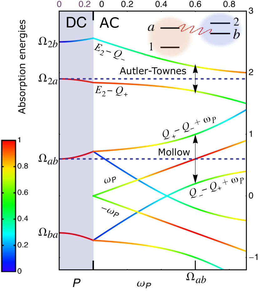
Figure 3: (Color online) Absorption energies as a function of the pump intensity $P\in[0,0.2]$ for $\omega_{P}=0$ [DC (grey) region] and as a function of $\omega_{P}\in[0,0.9]$ for $P=0.2$ [AC region] of a four-level quantum system consisting of the states $1,a\in A$ with energy $E_{1}=0$, $E_{a}=21.2$, and states $b,2\in B$ with energies $E_{b}=20.6$ $E_{2}=23.1$ (energies in eV). The absorption at energy $\Omega_{12}$ is independent of $P$ and not shown. The color scale indicates the oscillator strength of the transition [$\langle\Psi^{(0)}_{\alpha A}|\hat{d}|\Psi^{(1)}_{\gamma B}\rangle$ for $\Omega_{\alpha\gamma}+\omega_{P}$, $\langle\Psi^{(1)}_{\alpha B}|\hat{d}|\Psi^{(0)}_{\gamma A}\rangle$ for $\Omega_{\alpha\gamma}-\omega_{P}$, and the sum of the two for $\omega_{P}=0$, see Eq. (54)] normalized to $\mathfrak{D}\equiv\langle\Psi_{\alpha}|\hat{d}|\Psi_{\beta}\rangle$ with $\alpha=1,a$ and $\beta=b,2$. In the AC region we also display the absorption energy $\omega_{P}$ with oscillator strength $\sum_{\alpha}\langle\Psi^{(0)}_{\alpha A}|\hat{d}|\Psi^{(1)}_{\gamma B}\rangle$, and $-\omega_{P}$ with oscillator strength $\sum_{\alpha}\langle\Psi^{(1)}_{\alpha B}|\hat{d}|\Psi^{(0)}_{\gamma A}\rangle$.

We conclude this Section by discussing the paradigmatic situation of a pump coupling only two states, say $a$ and $b$. Then $P_{\alpha\beta}=P$ for $\alpha=a$ and $\beta=b$, and zero otherwise. The quasi-energies are

$$Q_{\pm}=\frac{E_{a}+E_{b}+\omega_{P}\pm\sqrt{(E_{a}-E_{b}-\omega_{P})^{2}+4P^{2}}}{2},$$ (55)

and for $\xi\neq a,b$, $Q_{\xi}=E_{\xi}$ for $\xi\in A$ and $Q_{\xi}=E_{\xi}+\omega_{P}$ for $\xi\in B$. In the limit of zero pump intensity $P\to 0$ the quasi-energies $Q_{+}\to E_{a}$ and $Q_{-}\to E_{b}+\omega_{P}$, as it should be. Let us analyze with the help of Fig. 3 the various time-dependent contributions in Eq. (54). For both $\alpha$ and $\gamma$ different from $\pm$ the square bracket is nonvanishing only provided that $\alpha\in A$ [$B$] and $\gamma\in B$ [$A$]. More precisely, only the first [second] term is nonvanishing, and it contributes with an oscillating exponential of frequency $E_{\alpha}-E_{\gamma}-\omega_{P}+\omega_{P}=E_{\alpha}-E_{\gamma}$ [$E_{\alpha}+\omega_{P}-E_{\gamma}-\omega_{P}=E_{\alpha}-E_{\gamma}$]. Thus, the absorption energy between “pump-invisible” states is preserved (and hence not shown in Fig. 3). The situation is more interesting for $\alpha\in A$ [$B$] a “pump-invisible” state and $\gamma=\pm$ , see Fig. 3 where the “pump-invisible” state is $\alpha=2\in B$. Again, only the first [second] term in the square bracket is nonvanishing and the corresponding oscillation frequency is $E_{\alpha}-Q_{\pm}+\omega_{P}$ [$E_{\alpha}-Q_{\pm}$]. We observe that for $P=0$ the quasi-eigenstate $|\Psi_{+}(t)\rangle=|\Psi_{a}\rangle$ is in the $A$ subspace whereas the quasi-eigenstate $|\Psi_{-}(t)\rangle=e^{i\omega_{P}t}|\Psi_{b}\rangle$ is in the $B$ subspace. Therefore the absorption at energy $E_{\alpha}-Q_{+}+\omega_{P}$ [$E_{\alpha}-Q_{-}$ (see the line $E_{2}-Q_{-}$ in Fig. 3)] is prohibited by the dipole selection rule. The pump field mixes $a$ and $b$, thereby giving rise to the appearance of a new peak for every equilibrium-forbidden transition between the “pump-invisible” state $\alpha\in B$ [$A$] and the state $b$ [$a$]. For $\omega_{P}$ far from the resonant frequency $\Omega_{ab}\equiv E_{a}-E_{b}$ the (allowed) equilibrium transition $E_{\alpha}-E_{b}\rightarrow E_{\alpha}-Q_{-}+\omega_{P}$ [$E_{\alpha}-E_{a}\rightarrow E_{\alpha}-Q_{+}$], thereby undergoing a shift known as the AC Stark shift.ste ; Bonch-Bruevich et al. (1969) At the resonance frequency $\omega_{P}=\Omega_{ab}$, the quasi-energies $Q_{\pm}=E_{a}\pm P$ and the equilibrium peak at $E_{\alpha}-E_{b}$ [$E_{\alpha}-E_{a}$] is replaced by two peaks of equal intensity at energy $E_{\alpha}-E_{b}\mp P$ [$E_{\alpha}-E_{a}\mp P$]. This spectral feature is known as the Autler-Townes doublet or splitting (since the original equilibrium peak appears split in two).Autler and Townes (1955); ste A similar analysis applies for $\alpha=\pm$ and $\gamma\in B$ [$A$] a “pump-invisible” state. Finally we consider the contributions with $\alpha=+$ and $\gamma=-$ [$\alpha=-$ and $\gamma=+$] in Eq. (54). In this case both terms in the square brackets contribute and the equilibrium peak at energy $\Omega_{ab}=E_{a}-E_{b}$ [$\Omega_{ba}=E_{b}-E_{a}$] splits into two peaks at energy $Q_{+}-Q_{-}\pm\omega_{P}$ [$Q_{-}-Q_{+}\pm\omega_{P}$], see Fig. 3. It is worth noticing that this splitting and the Autler-Townes splitting have different origin. In the latter a prohibited transition becomes an allowed transition whereas in the former a genuinely new transition appear. At the resonance frequency the spectrum exhibits two peaks of equal intensity at energies $Q_{+}-Q_{-}\pm\omega_{P}=2P\pm(E_{a}-E_{b})$ [$Q_{-}-Q_{+}\pm\omega_{P}=-2P\pm(E_{a}-E_{b})$]. Therefore, in this case too the equilibrium peak at energy $\Omega_{ab}$ [$\Omega_{ba}$] appears split in two. Unlike in the Autler-Townes splitting, however, the distance between the peaks is $4P$ instead of $2P$, with the peak at energy $\Omega_{ab}+2P$ [$\Omega_{ba}-2P$] stemming from a shift of the equilibrium peak at energy $\Omega_{ab}$ [$\Omega_{ba}$], and the peak at energy $\Omega_{ab}-2P$ [$\Omega_{ba}+2P$] stemming from the newly generated transition associated to the equilibrium peak at energy $\Omega_{ba}$ [$\Omega_{ab}$]. In addition to all the aforementioned absorption frequencies we have the pump frequency. In fact, for $\alpha=\gamma=\pm$ the square bracket in Eq. (54) is the sum of two oscillating exponentials with frequency $\pm\omega_{P}$. Thus, at the resonance frequency the spectrum exhibits a three-prong fork structure known as the Mollow triplet:Mollow (1969); ste the side peaks at energy $\Omega_{ab}\pm 2P$ [$\Omega_{ba}\pm 2P$] and a peak in the middle at energy $\omega_{P}=\Omega_{ab}$ [$-\omega_{P}=\Omega_{ba}$].

VI More analytic results and numerical simulations

The analysis of the nonequilibrium response function $\chi$ carried out in the previous Section is useful for the physical interpretation of TR-PA spectra. In practice, however, it is numerically more advantageous to calculate the probe induced dipole moment $d_{p}$ directly. In this Section we present some more analytic results for systems consisting of a few levels and single out the effects on the TR-PA spectrum of a finite duration of the pump.

Let $\underline{\rho}$ be the many-body density matrix in, e.g., the eigenbasis of the unperturbed Hamiltonian. The $(\alpha,\beta)$ matrix element of $\underline{\rho}$ is therefore $\langle\Psi_{\alpha}|\hat{\rho}|\Psi_{\beta}\rangle$. In the same basis the matrix which represents the unperturbed Hamiltonian is diagonal and reads $\underline{H}={\rm diag}(\{E_{\alpha}\})$. We use the convention that an underlined quantity $\underline{O}$ represents the matrix of the operator $\hat{O}$ in the energy eigenbasis. The time-evolution of the density matrix is determined by the Liouville equation

$$i\frac{d}{dt}\underline{\rho}(t)=[\underline{H}+\underline{H}_{P}(t)+\underline{H}_{p}(t),\underline{\rho}(t)]-\frac{i}{2}\{\underline{\Gamma},\underline{\rho}(t)\},$$ (56)

where $\underline{\Gamma}$ is a decay-rate matrix accounting for radiative, ionization and other decay-channels. In Eq. (56) the matrices $\underline{H}_{P}$ and $\underline{H}_{p}$ represent the pump and probe interaction Hamiltonians, and the symbol “$[\;,\;]$” (“$\{\;,\;\}$”) is a (anti)commutator. We set the switch-on time of the pump at $t=0$ (hence the probe is switched on at time $t=\tau$). As we are interested in the solution of Eq. (56) to lowest order in the probe field we write $\underline{\rho}=\underline{\rho}_{P}+\underline{\rho}_{p}$, where $\underline{\rho}_{P}(t)$ is the time-dependent density matrix with $\underline{H}_{p}=0$. Then, the probe-induced variation $\underline{\rho}_{p}$ satisfies (omitting the time argument)

$$i\frac{d}{dt}\underline{\rho}_{p}=[\underline{H}+\underline{H}_{P},\underline{\rho}_{p}]+[\underline{H}_{p},\underline{\rho}_{P}]-\frac{i}{2}\{\underline{\Gamma},\underline{\rho}_{p}\},$$ (57)

which should be solved with boundary condition $\underline{\rho}_{p}(\tau)=0$. For ultra-short probes $\underline{H}_{p}(t)=\delta(t-\tau)e_{0}\underline{d}$ and for times $t>\tau$ Eq. (57) simplifies to

$$i\frac{d}{dt}\underline{\rho}_{p}=[\underline{H}+\underline{H}_{P},\underline{\rho}_{p}]-\frac{i}{2}\{\underline{\Gamma},\underline{\rho}_{p}\},$$ (58)

which should be solved with boundary condition $\underline{\rho}_{p}(\tau)=-ie_{0}[\underline{d},\underline{\rho}_{P}(\tau)]$. Once $\underline{\rho}_{p}$ is known the probe-induced dipole moment can be calculated by tracing: $d_{p}={\rm Tr}[\underline{\rho}_{p}\underline{d}]$.

VI.1 Two-level system

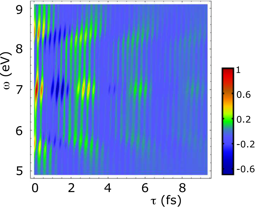
Figure 4: (Color online) TR-PA spectrum (normalized to the maximum) for the two level system described in the main text. The parameters are $\Omega_{ab}=E_{a}-E_{b}=7$, $P=0.7$, $\gamma_{a}=\gamma_{b}=\gamma=0.2$, $\gamma_{P}=0.02$ and $\omega_{P}=\Omega_{ab}$. Energies in eV and times in fs.

We consider a two-level system with unpertubed Hamiltonian $\underline{H}={\rm diag}(E_{a},E_{b})$, decay-rate matrix $\underline{\Gamma}={\rm diag}(\gamma_{a},\gamma_{b})$, and an exponentially decaying pump field which is suddenly switched-on at time $t=0$:

$$\underline{H}_{P}(t)=\theta(t)Pe^{-\gamma_{P}t}\left(\begin{array}[]{cc}0&e^{-i\omega_{P}t}\\ e^{i\omega_{P}t}&0\end{array}\right).$$ (59)

At time $t<0$ the state of the system is $|\Psi_{a}\rangle$ and hence the density matrix $\underline{\rho}_{P}(t<0)={\rm diag}(1,0)$. In Fig. 4 we show the TR-PA spectrum $\tilde{S}(\omega)$ for $\gamma_{P}\ll\gamma$, $\omega_{P}=\Omega_{ab}$ and for an ultra-short probe $\underline{H}_{p}(t)=\delta(t-\tau)e_{0}\underline{d}$, where the dipole matrix has off-diagonal elements $d_{ab}=d_{ba}=\mathfrak{D}$ and zero on the diagonal. The spectrum is calculated from Eq. (34) without the inclusion of the quadratic term in $d_{p}$ (thin samples). We clearly distinguish a Mollow triplet for small $\tau$. As the delay increases the side peaks approach the peak at $\omega_{P}$ and eventually merge with it. The $\tau$-dependent shift of the side peaks is a consequence of the finite duration of the pump. In the resonant case we have found a simple analytic solution for the probe-induced dipole moment (for simplicity we consider $\gamma_{a}=\gamma_{b}=\gamma$)

$$d_{p}(t)\!\! = \!\!2e_{0}\mathfrak{D}^{2}e^{-\gamma t}\big{[}\cos(\omega_{P}\tau)\sin(\omega_{P}t)\cos\big{(}2P\frac{1-e^{-\gamma_{P}t}}{\gamma_{P}}\big{)}$$ (60)

$$- \!\!\sin(\omega_{P}\tau)\cos\big{(}2P\frac{1-e^{-\gamma_{P}\tau}}{\gamma_{P}}\big{)}\cos(\omega_{P}t)\big{]},$$

for $t>\tau$ and zero otherwise. As the Fourier transform $\tilde{d}_{p}(\omega)$ is dominated by the behavior of $d_{p}(t)$ for times $\tau\leq t\lesssim 1/\gamma$ we study Eq. (60) in this range.

We write $t=\tau+s$ and define the function $\alpha(t)\equiv 2P(1-e^{-\gamma_{P}t})/\gamma_{P}$. For $\gamma_{P}\ll\gamma$ (this is the situation in Fig. 4) we can approximate

$$\alpha(t)=\alpha(\tau)+2Pe^{-\gamma_{P}\tau}s+\ldots$$ (61)

We then see that for a fixed $\tau$ the first term in the square brackets in Eq. (60) oscillates (as a function of $s$) at frequencies $\omega_{P}\pm 2Pe^{-\gamma_{P}\tau}$ whereas the second term oscillates at frequency $\omega_{P}$. This explains the shrinkage of the splitting between the two side peaks with increasing $\tau$ shown in Fig. 4. Another feature revealed by Eq. (60) is that the side-peak intensity is proportional to $\cos(\omega_{P}\tau)$ while the central-peak intensity is proportional to $\sin(\omega_{P}\tau)$ (antiphase). The Mollow triplet is therefore best visible only for delays $\tau=(2n+1)\pi/(4\omega_{P})$, with $n$ integers.

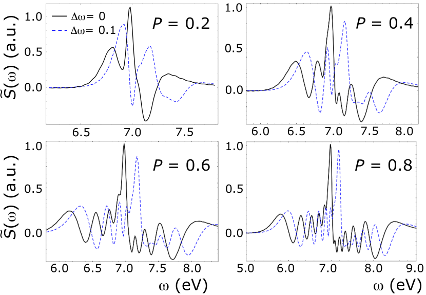
Figure 5: (Color online) TR-PA spectrum (normalized to the maximum) for the two level system described in the main text at a delay $\tau=\pi/4\omega_{P}$. The parameters are $\Omega_{ab}=E_{a}-E_{b}=7$, $\gamma_{a}=\gamma_{b}=\gamma_{P}=0.04$. Different panels refer to different pump intensity $P=0.2,\,0.4,\,0.6,\,0.8$ and the solid (dashed) line refers to the resonant (off-resonant) pump frequency $\omega_{P}=\Omega_{ab}+\Delta\omega$. Energies in eV.

Equation (60) is valid for arbitrary $\gamma$ and $\gamma_{P}$. Hence, it can be used to investigate regimes other than $\gamma_{P}\ll\gamma$. In the opposite regime $\gamma_{P}\gg\gamma$ we can approximate $\alpha(t)\simeq 2P/\gamma_{P}$, and only one peak at frequency $\omega_{P}$ is visible in the spectrum. The intermediate regime, $\gamma_{P}\gtrsim\gamma$, is definitely the most interesting as it is characterized by a nontrivial sub-splitting structure. In Fig. 5 we show the transient spectrum for $\gamma=\gamma_{P}=0.04$ at delay $\tau=\pi/(4\omega_{P})$ for different pump strengths $P$. The results are obtained from the solution of Eq. (58). We considered a resonant pump frequency, $\omega_{P}=\Omega_{ab}$, as well as an off-resonant one, $\omega_{P}=\Omega_{ab}+\Delta\omega$. Although an analytic formula for $d_{p}$ exists in the non-resonant case too, it is much less transparent than Eq. (60) and not worth it to present. After a careful study of Eq. (60) we found that the number of peaks in the frequency range $[-2P+\omega_{P},2P+\omega_{P}]$ grows roughly like $0.6\times P/\gamma_{P}$ and that the peak positions tend to accumulate around $\omega_{P}$ (in the limit $P/\gamma_{P}\rightarrow\infty$ the frequency $\omega_{P}$ becomes an accumulation point). The same qualitative behavior is observed for an off-resonant pump-frequency, the main difference being a shift by $\Delta\omega$ of the sub-splitting structure. The sub-peaks are probably the most remarkable feature of the complicated functional dependence of the TR-PA spectrum on the pump and probe fields. The sub-peaks are not related to transitions between light-dressed states and they can be observed only for pump pulses of duration comparable with the dipole decay time.

The full transient spectrum in the intermediate regime is shown in Fig. 6. We use the same parameters as in Fig. 5 and set the pump intensity $P=0.4$. Thus, for $\tau=\pi/(4\omega_{P})$ the spectrum is identical to the one shown in the top-right panel of Fig. 5. The sub-slitting structure evolves similarly as the main side-peaks. We observe periodic revivals of the sub-peaks whose positions get progressively closer to $\omega_{P}$ and whose intensities decrease with $\tau$. Another interesting feature is that for finite $\gamma_{P}$ the broadening of the peaks depends on $\tau$. It is therefore important to take into account the finite duration of the pump when estimating the excitation life-times from the experimental widths.

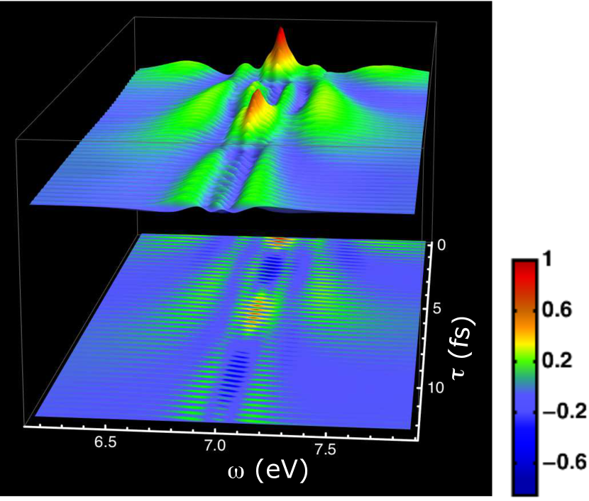
Figure 6: (Color online) TR-PA spectrum (normalized to the maximum) for the two level system described in the main text. The parameters are $\Omega_{ab}=E_{a}-E_{b}=7$, $\gamma_{a}=\gamma_{b}=\gamma_{P}=0.04$, $P=0.4$ and $\omega_{P}=\Omega_{ab}$. Energies in eV and times in fs.

VI.2 Three-level system

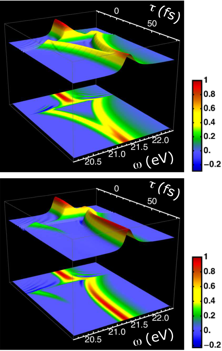
Figure 7: (Color online) TR-PA spectrum (normalized to the maximum) for the three level system described in the main text. The parameters are $E_{1}=0$, $E_{b}=20.6$, $E_{a}=21.2$, $P=0.7$, $\gamma=0.2$, $\gamma_{P}=0.04$ and $\omega_{P}=\Omega_{ab}$ (top panel) and $\omega_{P}=\Omega_{ab}-0.5$ (bottom panel). Energies in eV and time in fs.

We consider a three-level system with unperturbed Hamiltonian $\underline{H}={\rm diag}(E_{1},E_{b},E_{a})$ and decay-rate matrix $\underline{\Gamma}={\rm diag}(0,\gamma,\gamma)$. The system is perturbed by an exponentially decaying pump field which is suddenly switched-on at time $t=0$ and couples levels $a$ and $b$:

$$\underline{H}_{P}(t)=\theta(t)Pe^{-\gamma_{P}t}\left(\begin{array}[]{ccc}0&0&0\\ 0&0&e^{i\omega_{P}t}\\ 0&e^{-i\omega_{P}t}&0\end{array}\right).$$ (62)

In the absence of the probe the system is in the ground state $|\Psi_{1}\rangle$ before the pump is switched on, hence $\underline{\rho}_{P}(t<0)={\rm diag}(1,0,0)$. At time $\tau$ we switch on an ultrashort probe field $\underline{H}_{p}(t)=e(t)\underline{d}$ where $e(t)=e_{0}\delta(t-\tau)$ and, for simplicity, we take the dipole matrix of the form

$$\underline{d}=\left(\begin{array}[]{ccc}0&0&\mathfrak{D}\\ 0&0&0\\ \mathfrak{D}&0&0\end{array}\right)$$ (63)

(we therefore neglect the matrix element $\langle\Psi_{a}|\hat{d}|\Psi_{b}\rangle$). For $\omega_{P}\simeq E_{a}-E_{b}$ in the near-infrared region and $E_{a}-E_{1}$ in the extreme ultraviolet a similar model has been considered by several authors in studies of TR-PA of He atoms (in this case $1=1s^{2}$, $b=1s2s$, $a=1s2p$ represent the first three levels of He),Gaarde et al. (2011); Ranitovic et al. (2011); Chu and Lin (2012a); Pfeiffer and Leone (2012); Chen et al. (2012a); Pfeiffer et al. (2013); Chen et al. (2013a); Wu et al. (2013b); Chini et al. (2014) although the time-dependent probe and pump fields were different.

In Fig. 7 we show the TR-PA spectrum for a resonant (top panel) and off-resonant (bottom panel) pump frequency $\omega_{P}$. The spectrum is again calculated from Eq. (34) without the inclusion of the quadratic term in $d_{p}$ (thin samples). For negative $\tau$ we only see the equilibrium peak at frequency $\Omega_{a1}$, which corresponds to the excitation from the occupied level $1$ to the empty level $a$ (given the choice of the dipole matrix in Eq. (63) this is the only possible transition). For small positive $\tau$ we recognize the Autler-Townes splitting discussed in Section IV.2. The finite duration of the pump causes the collapse of the Autler-Townes splitting as $\tau$ increases; for $\tau\rightarrow\infty$ we eventually recover the equilibrium PA spectrum. The $\tau$-dependent shift of the Autler-Townes peaks can be study quantitatively in the resonant case. In fact, the differential equation for $\underline{\rho}_{p}$, see Eq. (58), can be solved analytically for $\omega_{P}=\Omega_{ab}$ and the corresponding probe-induced dipole moment reads

$$d_{p}(t) = \theta(t-\tau)2e_{0}\mathfrak{D}^{2}e^{-\gamma(t-\tau)}\sin\big{(}\Omega_{1a}(t-\tau)\big{)}$$ (64)

$$\times \cos\big{(}Pe^{-\gamma_{P}\tau}\frac{1-e^{-\gamma_{P}(t-\tau)}}{\gamma_{P}}\big{)}$$

Interestingly $d_{p}(\tau+s)$ depends on $\tau$ only through the exponentially renormalized pump intensity $Pe^{-\gamma_{P}\tau}$: the PA spectrum at finite $\tau$ and pump intensity $P$ is the same as the PA spectrum at $\tau=0$ and pump intensity $Pe^{-\gamma_{P}\tau}$. Therefore, the Autler-Townes splitting follows the exponential decay of the pump, in agreement with the numerical simulation in Fig. 7.

In the TR-PA spectrum of Fig. 7 we have $\gamma_{P}\ll\gamma$. However, the analytic solution in Eq. (64) is valid for all $\gamma$ and $\gamma_{P}$. Like in the two-level system a sub-splitting structure emerges in the intermediate regime $\gamma\simeq\gamma_{P}$ (not shown). A similar finding was recently found for trigonometric and square pump-envelops.Wu et al. (2013b)

The TR-PA spectra shown so far have been calculated under the assumption that the total electric probe field acting on the electrons is the same as the external (bare) field. As discussed in Section IV.2, this approximation makes sense for thin samples. For samples of thickness much larger than the inverse transition energies of interest, the Liouville equation for the density matrix, Eq. (56), should be coupled to the equation for the total electric field, Eq. (24).muk ; Ziolkowski et al. (1995); Buth et al. (2007); Gaarde et al. (2011); Chu and Lin (2012b); Chen et al. (2012b); Chu and Lin (2013); Wu et al. (2013a); Pfeiffer et al. (2013); Otobe et al. (2009); Yabana et al. (2012); Wachter et al. (2014); Deinega and Seideman (2014) To appreciate the qualitative difference introduced by a self-consistent treatment of the probe field we consider again the system of Fig. 7 and add to the bare $\delta$-like probe an induced exponentially decaying planewave of frequency $\Omega_{a1}$. We enforce (for simplicity) monochromaticity on the probe Hamiltonian (or equivalently we work in the rotating wave approximation) and take a total probe field $\mbox{\boldmath$\mathcal{E}$}_{p}(t)=(\mbox{$\mathcal{E}$}_{x}(t-\tau),\mbox{$\mathcal{E}$}_{y}(t-\tau),0)$, where the components

$$\mbox{$\mathcal{E}$}_{x}(t) = e_{0}\delta(t)+\theta(t)\lambda e^{-\gamma_{P}t}\cos\Omega_{a1}t$$

$$\mbox{$\mathcal{E}$}_{y}(t) = \theta(t)\lambda e^{-\gamma_{P}t}\sin\Omega_{a1}t$$ (65)

decay on the same time scale of the pump field. Choosing the dipole components $\underline{{\mathbf{d}}}=(\underline{d}_{x},\underline{d}_{y},\underline{d}_{z})$ with

$$\underline{d}_{x}=\left(\begin{array}[]{ccc}0&0&\mathfrak{D}\\ 0&0&0\\ \mathfrak{D}&0&0\end{array}\right)\quad;\quad\underline{d}_{y}=\left(\begin{array}[]{ccc}0&0&i\mathfrak{D}\\ 0&0&0\\ -i\mathfrak{D}&0&0\end{array}\right),$$ (66)

the probe Hamiltonian reads

$$\underline{H}_{p}(t)=\mbox{\boldmath$\mathcal{E}$}(t)\cdot\underline{{\mathbf{d}}}=\mathfrak{D}\left(\begin{array}[]{ccc}0&0&\mbox{$\mathcal{E}$}_{p}(t-\tau)\\ 0&0&0\\ \mbox{$\mathcal{E}$}^{\ast}_{p}(t-\tau)&&0\end{array}\right),$$ (67)

with $\mbox{$\mathcal{E}$}_{p}(t)=e_{0}\delta(t)+\theta(t)\lambda e^{i\Omega_{a1}t-\gamma_{P}t}$. Our modelling of the induced probe field is based on the self-consistent results of Ref. Pfeiffer et al., 2013. We instead assume that the pump field does not need to be dressed.

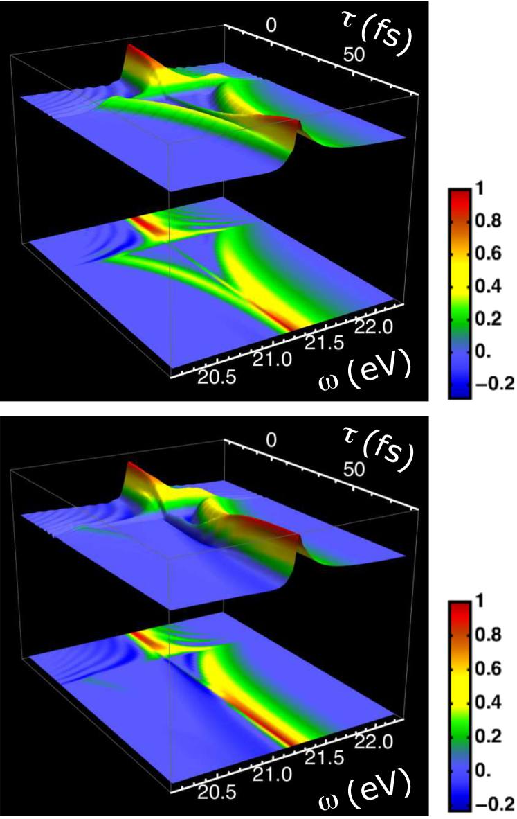
Figure 8: (Color online) Linear term in $d_{p}$ of the TR-PA spectrum (normalized to the maximum) of Eq. (34) for the three level system described in the main text. The probe Hamiltonian is given in Eq. (67) with $\lambda/e_{0}=0.01$. The rest of the parameters are the same as in Fig. 7. The pump frequency is $\omega_{P}=\Omega_{ab}$ (top panel) and $\omega_{P}=\Omega_{ab}-0.5$ (bottom panel). Energies in eV and time in fs.

The formula for the spectrum, Eq. (34), has beed derived for linearly polarized probe fields. It is straightforward to show that for ${\mathbf{e}}=\sum_{n}\mbox{\boldmath$\varepsilon$}_{p}^{(n)}e^{(n)}$ the generalization is

$$\tilde{S}(\omega)=-2\sum_{n}{\rm Im}\left(\!\omega\,\tilde{e}^{(n)\ast}(\omega)\tilde{d}^{(n)}_{p}(\omega)\!\right)-\frac{2\pi}{\mbox{$\mathcal{S}$}c}\left|\omega\,\tilde{{\mathbf{d}}}_{p}(\omega)\right|^{2}\!\!.$$ (68)

where $\tilde{d}^{(n)}_{p}\equiv\mbox{\boldmath$\varepsilon$}_{p}^{(n)}\cdot\tilde{d}^{(n)}_{p}$. In Fig. 8 we display the first term (linear in $d_{p}$) of the transient PA spectrum of Eq. (68). The main difference with the spectrum in Fig. 7 is the appearance of an extra peak at frequency $\Omega_{1a}$. It is therefore the induced probe field to generate the central peak. Furthermore, the height of the central peak increases monotonically (no coherent oscillations), in agreement with the results of Section IV.2. One more remark is about the exponential shrinkage of the Autler-Townes splitting already observed in Fig. 7. According to our calculations, the Autler-Townes splitting and the pump intensity decay on the same time-scale, see Eq. (64). This implies that a spectral shift can occur only provided that the amplitude of the pump field is delay dependent as is, for instance, the case in thick samples where the pump is dressed by an exponentially decaying dipole moment.

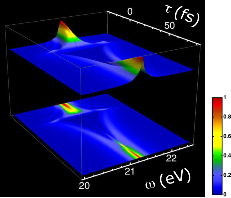
Figure 9: (Color online) Plot of $|\omega\,\bar{d}_{p}(\omega)|^{2}$ (normalized to the maximum) for the three level system described in the main text. Same parameters as in the top panel of Fig. 8. Energies in eV and time in fs.

For thick samples the quadratic term in $d_{p}$ in the TR-PA spectrum of Eq. (68) can become relevant. This term is always negative and hence it can either suppress a positive peak or even turn a positive peak into a negative one. The induced dipole moment scales linearly with the sample volume $V=\mbox{$\mathcal{S}$}L$. If we introduce the dipole density per unit volume $\bar{d}_{p}=d_{p}/V$, then the TR-PA spectrum in Eq. (68) can be rewritten as

$$\frac{\tilde{S}(\omega)}{V}=-2\sum_{n}{\rm Im}\left(\!\omega\,\tilde{e}^{(n)\ast}(\omega)\tilde{\bar{d}}^{(n)}_{p}(\omega)\!\right)-\frac{2\pi L}{c}\left|\omega\,\tilde{\bar{{\mathbf{d}}}}_{p}(\omega)\right|^{2}\!\!,\;\;$$ (69)

from which we see that the contribution of the last term grows linearly with the sample thickness. The quantity $|\omega\,\tilde{\bar{{\mathbf{d}}}}_{p}(\omega)|^{2}$ is shown in Fig. 9 in the resonant case $\omega_{P}=\Omega_{ab}$. As expected, the spectral regions where the linear (top panel of Fig. 8) and quadratic (Fig. 9) terms are nonvanishing are the same. Nevertheless, the mathematical structure of the peaks is very different, as it should be. In fact, in the absence of damping $\tilde{d}_{p}(\omega)$ is the sum of Dirac $\delta$-functions and hence its square is the sum of Dirac $\delta$-functions squared.

VII Summary and Conclusions

We have provided a detailed analysis of the nonequilibrium dipole response function $\chi$, the fundamental physical quantity to be calculated/simulated for interpreting TR-PA spectra. Exact and general properties of $\chi$ have been elucidated and then related to transient spectral features. In the nonoverlapping regime the height of the absorption peaks are strongly affected by the shape of the probe pulse. For ultrashort probes the peak heights exhibit quantum beats as a function of the delay, a signature of the coherent electron motion in the nonstationary state created by the pump. As the probe duration increases the effects of coherence are progressively washed out, and the spectrum is progressively suppressed away from the probe frequency. The absorption regions are instead independent of the delay and occur in correspondence of the neutral excitation energies (not necessarily involving the ground-state) of the equilibrium system. For overlapping pump and probe the absorption regions cease to be an intrinsic property of the equilibrium system and, more generally, the interpretation of the transient spectrum becomes intricate. Analytic results for everlasting periodic pump fields are available and at the same time useful for the interpretation of TR-PA spectra. The Lehmann-like representation of $\chi$ in terms of light-dressed states provide a unifying framework for a variety of well known phenomena, e.g., the AC-Stark shift, the Autler-Townes splitting, the Mollow triplet, the photon replicas, etc.

The effects of the finite duration of the pump pulse are difficult to address in general terms. We have considered the two- and three-level systems extensively studied in the literature and derived an exact analytic expression for the time-dependent probe-induced dipole moment. Our solution shows that for strong enough pump intensities a rich sub-splitting structure emerges, in agreement with the recent theoretical findings in Ref. Wu et al., 2013b. We also find agreement with recent experimental results on He: for long (induced) probe fields, like those occurring in thick samples, the absorption peak at the probe frequency does not exhibit coherent oscillations.Pfeiffer et al. (2013)

References

- Krausz and Ivanov (2009) F. Krausz and M. Ivanov, Rev. Mod. Phys. 81, 163 (2009).
- Berera et al. (2009) R. Berera, R. van Grondelleand, and J. T. M. Kennis, Photosynth. Res. 101, 105 (2009).
- Gallmann et al. (2012) L. Gallmann, C. Cirelli, and U. Keller, Annu. Rev. Phys. Chem. 63, 447 (2012).
- Sansone et al. (2012) G. Sansone, T. Pfeifer, K. Simeonidis, and A. I. Kuleff, Chem. Phys. Chem. 13, 661 (2012).
- Gallmann et al. (2013) L. Gallmann, J. Herrmann, R. Locher, M. Sabbar, A. Ludwig, M. Lucchini, and U. Keller, Mol. Phys. 111, 2243 (2013).
- Kuleff and Cederbaum (2014) A. I. Kuleff and L. S. Cederbaum, J. Phys. B: At. Mol. Opt. Phys. 47, 124002 (2014).
- Kaindl et al. (2003) R. A. Kaindl, M. A. Carnahan, D. Hägele, R. Lövenich, and D. S. Chemla, Nature 423, 734 (2003).
- Wang et al. (2005) F. Wang, G. Dukovic, L. E. Brus, and T. F. Heinz, Science 308, 838 (2005).
- Koch et al. (2006) S. W. Koch, M. Kira, G. Khitrova, and H. M. Gibbs, Nat. Mater. 5, 523 (2006).
- Piris et al. (2009) J. Piris, T. E. Dykstra, A. A. Bakulin, P. H. M. van Loosdrecht, W. Knulst, M. T. Trinh, J. M. Schins, and L. D. A. Siebbeles, J. Phys. Chem. C 113, 14500 (2009).
- Cowan et al. (2012) S. R. Cowan, N. Banerji, W. L. Leong, and A. J. Heeger, Adv. Funct. Mater. 22, 1116 (2012).
- (12) V. May and O. Kühn, Charge and energy transfer dynamics in molecular systems (John Wiley & Sons, Weinheim, 2004).
- Asbury et al. (2000) J. B. Asbury, E. Hao, Y. Wang, and T. Lian, J. Phys. Chem. B 104, 11957 (2000).
- Schnadt et al. (2002) J. Schnadt, P. A. Brühwiler, L. Patthey, J. N. O’Shea, S. Södergren, M. Odelius, R. Ahuja, O. Karis, M. Bässler, P. Persson, et al., Nature 418, 620 (2002).
- Föhlisch et al. (2005) A. Föhlisch, P. Feulner, F. Hennies, A. Fink, D. Menzel, D. Sanchez-Portal, P. M. Echenique, and W. Wurth, Nature 436, 373 (2005).
- Gray and Winkler (2005) H. B. Gray and J. R. Winkler, Proc. Natl. Acad. Sci. U.S.A 102, 3534 (2005).
- Remacle and Levine (2006) F. Remacle and R. D. Levine, Proc. Natl. Acad. Sci. U.S.A. 103, 6793 (2006).
- Rozzi et al. (2013) C. A. Rozzi, S. M. Falke, N. Spallanzani, A. Rubio, E. Molinari, D. Brida, M. Maiuri, G. Cerullo, H. Schramm, J. Christoffers, et al., Nature Comm. 4, 1602 (2013).
- Falke et al. (2014) S. M. Falke, C. A. Rozzi, D. Brida, M. Maiuri, M. Amato, E. Sommer, A. D. Sio, A. Rubio, G. Cerullo, E. Molinari, et al., Science 344, 1001 (2014).
- (20) S. Pittalis and A. Delgado and J. Robin and L. Freimuth and J. Christoffers and C. Lienau and C.A. Rozzi, Adv. Func. Mater. DOI: 10.1002/adfm.201402316 (2015).
- Pfeiffer et al. (2011) A. N. Pfeiffer, C. Cirelli, M. Smolarski, R. Dörner, and U. Keller, Nature Phys. 7, 428 (2011).
- Bernhardt et al. (2014a) B. Bernhardt, A. R. Beck, X. Li, E. R. Warrick, M. J. Bell, D. J. Haxton, C. W. McCurdy, D. M. Neumark, and S. R. Leone, Phys. Rev. A 89, 023408 (2014a).
- Buth et al. (2007) C. Buth, R. Santra, and L. Young, Phys. Rev. Lett. 98, 253001 (2007).
- Glover et al. (2010) T. E. Glover, M. P. Hertlein, S. H. Southworth, T. K. Allison, J. van Tilborg, E. P. Kanter, B. Krässig, H. R. Varma, B. Rude, R. Santra, et al., Nature Phys. 6, 69 (2010).
- Gilbertson et al. (2010) S. Gilbertson, M. Chini, X. Feng, S. Khan, Y. Wu, and Z. Chang, Phys. Rev. Lett. 105, 263003 (2010).
- Ranitovic et al. (2011) P. Ranitovic, X. M. Tong, C. W. Hogle, X. Zhou, Y. Liu, N. Toshima, M. M. Murnane, and H. C. Kapteyn, Phys. Rev. Lett. 106, 193008 (2011).
- Tarana and Greene (2012) M. Tarana and C. H. Greene, Phys. Rev. A 85, 013411 (2012).
- Lin et al. (2012) M.-F. Lin, A. N. Pfeiffer, D. M. Neumark, O. Gessner, and S. R. Leone, J. Chem. Phys. 137, 244305 (2012).
- Chen et al. (2012a) S. Chen, M. J. Bell, A. R. Beck, H. Mashiko, M. Wu, A. N. Pfeiffer, M. B. Gaarde, D. M. Neumark, S. R. Leone, and K. J. Schafer, Phys. Rev. A 86, 063408 (2012a).
- Chini et al. (2012) M. Chini, B. Zhao, H. Wang, Y. Cheng, S. X. Hu, and Z. Chang, Phys. Rev. Lett. 109, 073601 (2012).
- Chen et al. (2013a) S. Chen, M. Wu, M. B. Gaarde, and K. J. Schafer, Phys. Rev. A 87, 033408 (2013a).
- Chen et al. (2013b) S. Chen, M. Wu, M. B. Gaarde, and K. J. Schafer, Phys. Rev. A 88, 033409 (2013b).
- Herrmanna et al. (2013) J. Herrmanna, M. Weger, R. Locher, P. R. M. Sabbar, U. Saalmann, J.-M. Rost, L. Gallmann, and U. Keller, Phys. Rev. A 88, 043843 (2013).
- Chini et al. (2013) M. Chini, X. Wang, Y. Cheng, Y. Wu, D. Zhao, D. A. Telnov, S.-I. Chu, and Z. Chang, Scientific Reports 3, 1105 (2013).
- Pfeiffer et al. (2013) A. N. Pfeiffer, M. J. Bell, A. R. Beck, H. Mashiko, D. M. Neumark, and S. R. Leone, Phys. Rev. A 88, 051402 (2013).
- Wang et al. (2013) X. Wang, M. Chini, Y. Cheng, Y. Wu, X.-M. Tong, and Z. Chang, Phys. Rev. A 87, 063413 (2013).
- Bernhardt et al. (2014b) B. Bernhardt, A. R. Beck, E. R. Warrick, M. Wu, S. Chen, M. B. Gaarde, K. J. Schafer, D. M. Neumark, and S. R. Leone, New J. Phys. 16, 113016 (2014b).
- Wickenhauser et al. (2005) M. Wickenhauser, J. Burgdörfer, F. Krausz, and M. Drescher, Phys. Rev. Lett. 94, 023002 (2005).
- Zhao and Lein (2012) J. Zhao and M. Lein, New J. Phys. 14, 065003 (2012).
- Chu and Lin (2013) W. Chu and C. D. Lin, Phys. Rev. A 87, 013415 (2013).
- Ott et al. (2013) C. Ott, A. Kaldun, P. Raith, K. Meyer, M. Laux, J. Evers, C. H. Keitel, C. H. Greene, and T. Pfeifer, Science 340, 716 (2013).
- Ott et al. (2014) C. Ott, A. Kaldun, L. Argenti, P. Raith, K. Meyer, M. Laux, Y. Zhang, A. Blättermann, S. Hagstotz, T. Ding, et al., Nature 516, 374 (2014).
- Argenti et al. (2014) L. Argenti, C. Ott, T. Pfeifer , and F. Martín, J. Phys.: Conf. Ser. 488, 032030 (2014).
- Huber et al. (2001) R. Huber, F. Tauser, A. Brodschelm, M. Bichler, G. Abstreiter, and A. Leitenstorfer, Nature 414, 286 (2001).
- Hase et al. (2003) M. Hase, M. Kitajima, A. M. Constantinescu, and H. Petek, Nature 426, 51 (2003).
- Borisov et al. (2004) A. Borisov, D. Sánchez-Portal, R. Muio, and P. Echenique, Chem. Phys. Lett. 387, 95 (2004).
- Moskalenko et al. (2012) A. S. Moskalenko, Y. Pavlyukh, and J. Berakdar, Phys. Rev. A 86, 013202 (2012).
- Srivastava et al. (2004) A. Srivastava, R. Srivastava, J. Wang, and J. Kono, Phys. Rev. Lett. 15, 157401 (2004).
- Nagler and et al. (2009) B. Nagler and et al., Nature Phys. 5, 693 (2009).
- Drescher et al. (2002) M. Drescher, M. Hentschel, R. Kienberger, M. Uiberacker, V. Yakovlev, A. Scrinzi, T. Westerwalbesloh, U. Kleineberg, U. Heinzmann, and F. Krausz, Nature 419, 803 (2002).
- Niikura et al. (2005) H. Niikura, D. M. Villeneuve, and P. B. Corkum, Phys. Rev. Lett. 94, 083003 (2005).
- Smirnova et al. (2009) O. Smirnova, Y. Mairesse, S. Patchkovskii, N. Dudovich, D. Villeneuve, P. Corkum, and M. Y. Ivanov, Nature 460, 972 (2009).
- Smirnovaa et al. (2009) O. Smirnovaa, S. Patchkovskiia, Y. Mairessea, N. Dudovich, and M. Y. Ivanov, Proc. Natl. Acad. Sci. U.S.A 106, 16556 (2009).
- Goulielmakis et al. (2010) E. Goulielmakis, Z. Loh, A. Wirth, R. Santra, N. Rohringer, V. S. Yakovlev, S. Zherebtsov, T. Pfeifer, A. M. Azzeer, M. F. Kling, et al., Nature 466, 739 (2010).
- Pabst et al. (2011) S. Pabst, L. Greenman, P. J. Ho, D. A. Mazziotti, and R. Santra, Phys. Rev. Lett. 106, 053003 (2011).
- Breusing et al. (2009) M. Breusing, C. Ropers, and T. Elsaesser, Phys. Rev. Lett. 102, 086809 (2009).
- Schultze et al. (2013) M. Schultze, E. M. Bothschafter, A. Sommer, S. Holzner, W. Schweinberger, M. Fiess, M. Hofstetter, R. Kienberger, V. Apalkov, V. S. Yakovlev, et al., Nature 493, 75 (2013).
- Schultze et al. (2014) M. Schultze, K. Ramasesha, C. D. Pemmaraju, A. Sato, D. Whitmore, A. Gandman, J. S. Prell, L. J. Borja, D. Prendergast, K. Yabana, et al., Science 346, 1348 (2014).
- Zewail (2000) A. H. Zewail, J. Phys. Chem. A 104, 5660 (2000).
- Chen (2005) L. Chen, Annu. Rev. Phys. Chem. 56, 221 (2005).
- Sansone et al. (2010) G. Sansone, F. Kelkensberg, J. F. Pérez-Torres, F. Morales, M. F. Kling, W. Siu, O. Ghafur, P. Johnsson, M. Swoboda, E. Benedetti, et al., Nature 465, 763 (2010).
- Lawrence and Skinner (2003) C. P. Lawrence and J. L. Skinner, Chem. Phys. Lett. 369, 472 (2003).
- Cavalieri et al. (2007) A. L. Cavalieri, N. Müller, T. Uphues, V. S. Yakovlev, A. Baltuska, B. Horvath, B. Schmidt, L. Blümel, R. Holzwarth, S. Hendel, et al., Nature 449, 1029 (2007).
- Wang et al. (2010) H. Wang, M. Chini, S. Chen, C.-H. Zhang, F. He, Y. C. andY. Wu, U. Thumm, and Z. Chang, Phys. Rev. Lett. 105, 143002 (2010).
- Holler et al. (2011) M. Holler, F. Schapper, Gallmann, and U. Keller, Phys. Rev. Lett. 106, 123601 (2011).
- (66) F. Bassani and G. Pastori-Parravicini, Electronic States and Optical Transitions in Solids (Pergamon Press, NY, 1975).
- Strinati (1988) G. Strinati, Riv. Nuovo Cimento 11, 1 (1988).
- (68) G. Giuliani and G. Vignale, Quantum theory of the electron liquid (Cambridge University Press, Cambridge, 2005).
- (69) G. Stefanucci and R. van Leeuwen, Nonequilibrium Many-Body Theory of Quantum Systems: A Modern Introduction (Cambridge University Press, Cambridge, 2013).
- Gaarde et al. (2011) M. B. Gaarde, C. Buth, J. L. Tate, and K. J. Schafer, Phys. Rev. A 83, 013419 (2011).
- Santra et al. (2011) R. Santra, V. S. Yakovlev, T. Pfeifer, and Z. Loh, Phys. Rev. A 83, 033405 (2011).
- Chu and Lin (2012a) W. Chu and C. D. Lin, Phys. Rev. A 85, 013409 (2012a).
- Baggesen et al. (2012) J. C. Baggesen, E. Lindroth, and L. B. Madsen, Phys. Rev. A 85, 013415 (2012).
- Dutoi et al. (2013) A. D. Dutoi, K. Gokhberg, and L. S. Cederbaum, Phys. Rev. A 88, 013419 (2013).
- (75) S. Mukamel, Principles of Nonlinear Optical Spectroscopy (Oxford University Press, Oxford, 1995).
- (76) E. Perfetto, D. Sangalli, A. Marini and G. Stefanucci, unpublished.
- Bertsch et al. (2000) G. F. Bertsch, J.-I. Iwata, A. Rubio, and K. Yabana, Phys Rev. B 62, 7998 (2000).
- Sun et al. (2007) J. Sun, J. Song, Y. Zhao, and W.-Z. Liang, J. Chem. Phys. 127, 234107 (2007).
- Kwong and Bonitz (2000) N.-H. Kwong and M. Bonitz, Phys. Rev. Lett. 84, 1768 (2000).
- Dahlen and van Leeuwen (2007) N. E. Dahlen and R. van Leeuwen, Phys. Rev. Lett. 98, 153004 (2007).
- von Friesen et al. (2009) M. P. von Friesen, C. Verdozzi, and C.-O. Almbladh, Phys. Rev. Lett. 103, 176404 (2009).
- Attaccalite et al. (2011) C. Attaccalite, M. Grüning, and A. Marini, Phys. Rev. B 84, 245110 (2011).
- Myöhänen et al. (2012) P. Myöhänen, R. Tuovinen, T. Korhonen, G. Stefanucci, and R. van Leeuwen, Phys. Rev. B 85, 075105 (2012).
- Latini et al. (2014) S. Latini, , E. Perfetto, A.-M. Uimonen, R. van Leeuwen, and G. Stefanucci, Phys. Rev. B 89, 075306 (2014).
- De Giovannini et al. (2013) U. De Giovannini, G. Brunetto, A. Castro, J. Walkenhorst, and A. Rubio, Chem. Phys. Chem 14, 1363 (2013).
- Neidel et al. (2013) C. Neidel, J. Klei, C.-H. Yang, A. Rouzée, M. J. J. Vrakking, K. Klünder, M. Miranda, C. L. Arnold, T. Fordell, A. L’Huillier, et al., Phys. Rev. Lett. 111, 033001 (2013).
- Crawford-Uranga et al. (2014) A. Crawford-Uranga, U. D. Giovannini, E. Räsänen, M. J. T. Oliveira, D. J. Mowbray, G. M. Nikolopoulos, E. T. Karamatskos, D. Markellos, P. Lambropoulos, S. Kurth, et al., Phys. Rev. A 90, 033412 (2014).
- (88) R. Loudon, The quantum Theory of Light (Clarendon Press, Oxford, 2000).
- not (a) For thick samples the total field is not spatially uniform and Eq. (35) involves an integral over space too.
- Ziolkowski et al. (1995) R. W. Ziolkowski, J. M. Arnold, and D. M. Gogny, Phys. Rev. A 52, 3082 (1995).
- Chu and Lin (2012b) W. Chu and C. D. Lin, J. Phys. B: At. Mol. Opt. Phys. 45, 201002 (2012b).
- Chen et al. (2012b) S. Chen, K. J. Schafer, and M. B. Gaarde, Opt. Lett. 37, 2211 (2012b).
- Wu et al. (2013a) M. Wu, S. Chen, K. J. Schafer, and M. B. Gaarde, Phys. Rev. A 87, 013828 (2013a).
- Otobe et al. (2009) T. Otobe, K. Yabana, and J.-I. Iwata, J. Phys. Condens. Matter 21, 064224 (2009).
- Yabana et al. (2012) K. Yabana, T. Sugiyama, Y. Shinohara, T. Otobe, and G. F. Bertsch, Phys. Rev. B 85, 045134 (2012).
- Wachter et al. (2014) G. Wachter, C. Lemell, J. Burgdörfer, S. A. Sato, X.-M. Tong, and K. Yabana, Phys. Rev. Lett 113, 087401 (2014).
- Deinega and Seideman (2014) A. Deinega and T. Seideman, Phys. Rev. A 89, 022501 (2014).
- Shirley (1965) J. H. Shirley, Phys. Rev. 138, B979 (1965).
- (99) L. Allen and J. H. Eberly, Optical Resonance and Two-Level Atoms (Dover Publications, New York, 1987).
- (100) P. Meystre, Atom Optics (Springer-Verlag, New York, 2001).
- (101) R. W. Boyd, Nonlinear Optics (Academic Press, Boston, 1992).
- (102) C. Cohen-Tannoudji, J. Dupont-Roc, and G. Grynberg, Atom-Photon Interactions: Basic Processes and Applications (John Wiley & Sons, New York, 1992).
- Kitagawa et al. (2011) T. Kitagawa, T. Oka, A. Brataas, L. Fu, and E. Demler, Phys. Rev. B 84, 235108 (2011).
- Li et al. (2014) Y. Li, A. Kundu, F. Zhong, and B. Seradjeh, Phys. Rev. B 90, 121401 (2014).
- not (b) The same result follows from the direct solution of the Schrödinger equation . Projecting this equation onto subspaces and one finds and . Writing the problem is mapped onto a Schrödinger equation for time-independent Hamiltonians: .
- (106) D. A. Steck, Quantum and Atom Optics (available online at http://steck.us/teaching).
- Bonch-Bruevich et al. (1969) A. M. Bonch-Bruevich, N. N. Kostin, V. A. Khodovoi, and V. V. Khromov, Sov. Phys. JETP 29, 82 (1969).
- Autler and Townes (1955) S. H. Autler and C. H. Townes, Phys. Rev. 100, 703 (1955).
- Mollow (1969) B. R. Mollow, Phys. Rev. 188, 1969 (1969).
- Pfeiffer and Leone (2012) A. N. Pfeiffer and S. R. Leone, Phys. Rev. A 85, 053422 (2012).
- Wu et al. (2013b) M. Wu, S. Chen, M. B. Gaarde, and K. J. Schafer, Phys. Rev. A 88, 043416 (2013b).
- Chini et al. (2014) M. Chini, X. Wang, Y. Cheng, and Z. Chang, J. Phys. B: At. Mol. Opt. Phys. 47, 124009 (2014).