Existence and Stability of Periodic Orbits in $N$-Dimensional Piecewise Linear Continuous Maps

Abstract

Piecewise smooth maps are known to exhibit a wide range of dynamical features including numerous types of periodic orbits. Predicting regions in parameter space where such periodic orbits might occur and determining their stability is crucial to characterize the dynamics of the system. However, obtaining the conditions of existence and stability of these periodic orbits generally use brute force methods which require successive application of the iterative map on a starting point. In this article, we propose a faster and more elegant way of obtaining those conditions without iterating the complete map. The method revolves around direct computation of higher powers of matrices without computing the lower ones and is applicable on any dimension of the phase space. In the later part of the article, we compare the speed of the proposed method with the other popular algorithms which shows the effectiveness of the proposed method in higher dimensions. We also illustrate the use of this method in computing the regions of existence and stability of a particular class of periodic orbits in three dimensions.

I Introduction

Presence of stable and unstable periodic orbits play a vital role in determining the dynamical properties of a system. While presence of stable periodic orbits form the basins of attraction, the unstable periodic orbits play a crucial role in forming chaotic orbits and the basin boundaries of the attractors. In fact appearance, disappearance or change in stability of these periodic orbits are responsible for most bifurcation phenomena. Hence an important component in characterising a given system is determining the parameters for which a particular periodic orbit might exist.

Piecewise smooth maps are useful in describing systems whose evolution is given by different smooth functions in different regions of space. Examples of piecewise smooth systems include switching electrical circuits Deane and Hamill (1990); Kousaka et al. (1999), impacting mechanical systems Nordmark (1991), walking robots Thuilot et al. (1997); Garcia et al. (1998), cardiac dynamics Sun et al. (1995) and neural spiking Börgers and Kopell (2003). Apart from their applicability, piecewise smooth maps have also attracted attention due to their rich dynamical properties. Even maps which are piecewise linear and have non-linearities only across a switching manifold, exhibit features like robust chaos Banerjee et al. (1998) and existence of infinitely many co-existing attractors Simpson (2014). Study of piecewise linear maps attains even more importance as they can describe the behaviour of the piecewise smooth systems near the border separating the partitions of the phase space, in which case the matrices take a specific form. This article aims to study the conditions of existence and stability of periodic orbits in such piecewise linear maps in any arbitrary dimension.

Periodic orbits in piecewise linear one, two and three dimensional maps have been studied Nusse and Yorke (1992); Roy and Roy (2008); Avrutin et al. (2012). Some of the works have also computed the regions in parameter space where specific types of orbits exist and are stable Avrutin et al. (2012); Gardini et al. (2010); Ganguli and Banerjee (2005); Panchuk et al. (2015). However most of the studies used repeated application of the iterative map to obtain them. An iterative technique, invented by the Russian mathematician Leonov Leonov (1959, 1962); Panchuk et al. (2015) has also been used to obtain the existence condition of periodic orbits Gardini et al. (2010); Avrutin et al. (2010); Tramontana et al. (2012). Moreover, the methods used there were specific to the type of orbit being analysed.

In this work, we seek to obtain a generic and faster method of finding the existence and stability criteria for a general class of periodic orbits. The technique developed might be extended to any periodic obit in piecewise linear maps of any dimension. Moreover, as the technique is essentially an algorithm to obtain higher iterates of the map without going through the intermediate ones, it can be used to simplify extraction of other relevant information about the map. Additionally, the maps we work on are in their normal forms. Hence the ambit of the results obtained spreads across all piecewise smooth maps as appropriate coordinate transformation near the border of non-smoothness yields the normal form of the maps.

The paper is organized as follows. After defining the notations and conventions used in the article in the Section-2, we derive the generic conditions for existence and stability of periodic orbits in a dimension independent form. We then develop a technique which exploits the form of the map to obtain the conditions of existence and stability in $N$ dimensions. We showcase the utility of the technique developed by computing the parameter regions in which certain classes of stable periodic orbits exist in a three dimensional piecewise linear map in the next section. Thereafter, we take the specific case of two dimensional systems, where the simplicity of the map allows us to obtain stronger analytical results. Finally, we devote a section to exhibit the computational efficiency of the technique developed by comparing it with other traditionally used methods for computing the existence and stability criteria of periodic orbits in piecewise linear maps.

II The Piecewise Linear Map in the Normal Form

In earlier literature it has been shown that, on proper choice of axes, any $N$ dimensional piecewise smooth continuous map can be linearised near the border to have the following form Nusse and Yorke (1992)

$$G_{\mu}(X)=\left\{\begin{array}[]{lr}M_{L}X+\zeta&:x_{1}\leq 0\\ {}&{}\hfil\\ M_{R}X+\zeta&:x_{1}>0\end{array}\right.$$ (1)

where $M_{L},M_{R}\in\mathbb{R}^{N\times N}$ are matrices in their normal form given by di Bernardo (2003)

$$M_{J}=\begin{pmatrix}-d^{(J)}_{1}&1&0&\cdots&0\\ -d^{(J)}_{2}&0&1&\cdots&0\\ \vdots&\vdots&\vdots&\cdots&\vdots\\ -d^{(J)}_{N-1}&0&0&\cdots&1\\ -d^{(J)}_{N}&0&0&\cdots&0\end{pmatrix}~{}~{}~{}:J\in\left\{L,R\right\}$$ (2)

with $d^{(J)}_{i}$ being the coefficient of $\lambda^{i}$ in the characteristic polynomial of $M_{J}$; $X=\left(x_{1},\ldots,x_{N}\right)^{T}\in\mathbb{R}^{N}$ being a generic point in the phase space and $\zeta=\left(\mu,\ldots,0\right)^{T}$. Since the coefficient of $\lambda^{i}$ in the characteristic polynomial of a matrix is the sum of eigenvalues of the matrix taken $i$ at a time (apart from an alternating sign); we recast (2) as

$$M_{J}=\begin{pmatrix}\rho^{(J)}_{1}&1&0&\cdots&0\\ -\rho^{(J)}_{2}&0&1&\cdots&0\\ \vdots&\vdots&\vdots&\cdots&\vdots\\ (-1)^{N-2}~{}\rho^{(J)}_{N-1}&0&0&\cdots&1\\ (-1)^{N-2}~{}\rho^{(J)}_{N}&0&0&\cdots&0\end{pmatrix}~{}~{}~{}:J\in\left\{L,R\right\}$$ (3)

for further analysis. Here $\rho^{(J)}_{i}$ is the sum of the eigenvalues of $M_{J}$ taken $i$ at a time, i.e., $\rho^{(J)}_{i}=(-1)^{i-1}d^{(J)}_{i}$. For instance, in two and three dimensions, the matrix in (3) takes the form,

$$M_{J}=\begin{pmatrix}\tau_{J}&1\\ -\delta_{J}&0\end{pmatrix}~{}~{}~{}:J\in\left\{L,R\right\}$$ (4)

and

$$M_{J}=\begin{pmatrix}\tau_{J}&1&0\\ -\sigma_{J}&0&1\\ \delta_{J}&0&0\end{pmatrix}~{}~{}~{}:J\in\left\{L,R\right\}$$ (5)

respectively. Here $\tau_{J}$ and $\delta_{J}$ are the trace and determinant the $M_{J}$; and $\sigma_{J}$ is the sum of the eigenvalues of $M_{J}$ taken two at a time.

Any $p$-periodic orbit in such a system can be represented by a sequence of points $\left\{X_{0},\ldots,X_{i},\ldots,X_{p-1}\right\}$ such that $X_{i+1}=G_{\mu}(X_{i})$ where $i$ is a natural number or zero, and $X_{p}=X_{0}$. We can also associate a symbol to each point on the periodic orbit depending on the partition in which it lies. If a point of the periodic orbit has $x_{1}\leq 0$, it is assigned the symbol $L$ (meaning left). Otherwise it is assigned the symbol $R$ (meaning right). This associates a sequence of $R$ and $L$ to each periodic orbit. For example, an $LLLR$ (also written as $L^{3}R$) orbit consists of three points with $x_{1}\leq 0$ and a single point with $x_{1}>0$. To remove the ambiguity arising from possible cyclic permutation of the points, in this article we adopt the following convention: We number the points $X_{i}$ such that $X_{0}$ is assigned the symbol $R$ and $X_{p}$ is assigned the symbol $L$. However while referring of the orbits, we collect the symbols in the reverse order such that the symbol for the orbit starts with $L$ and ends with $R$. In this article, for sake of simplicity, we would restrict our explicit analysis to orbits of the form $L^{m}R^{n}$ where $m$ and $n$ are natural numbers. However, the theory developed here can be extended to the general finite period orbit $L^{n_{1}}R^{n_{2}}\ldots L^{n_{s-1}}R^{n_{s}}$. Ways to extend the theory for the general cases will be indicated wherever required. Note that since the map in each of the partitions is linear, a periodic orbit lying completely within any one of the partitions does not exist.

III Existence and Stability of Periodic Orbits

In 1959, Leonov Leonov (1959, 1962) did a detailed study of nested period adding bifurcation structure occurring in piecewise-linear discontinuous 1D maps. The algorithmic way proposed in his work was recently usedGardini et al. (2010) to analyse border collision bifurcations in one dimensional maps. We extend the analysis to obtain the existence criteria for period orbits in $N$ dimensions.

Consider an $L^{m}R^{n}$ orbit formed by the points $\left\{X_{0},\ldots,X_{m+n-1}\right\}$. According to the convention described in the last section, we assume the points $X_{0},\ldots,X_{m-1}$ have $x_{1}>0$ and the points $X_{m},\ldots,X_{m+n-1}$ have $x_{1}\leq 0$. Hence the evolution of $X_{0}$ under the map $G_{\mu}$ is given as,

$$X_{1} =M_{R}X_{0}+\zeta$$

$$X_{2} =M_{R}^{2}X_{0}+\left(I+M_{R}\right)\zeta$$

$$X_{3} =M_{R}^{3}X_{0}+\left(I+M_{R}+M_{R}^{2}\right)\zeta$$

$$\vdots ~{}~{}~{}~{}~{}~{}~{}~{}~{}~{}\vdots$$

$$X_{n-1} =M_{R}^{n-1}X_{0}+\phi_{R,n-1}\zeta$$

$$X_{n} =M_{R}^{n}X_{0}+\phi_{R,n}\zeta$$

$$X_{n+1} =M_{L}M_{R}^{n}X_{0}+M_{L}\phi_{R,n}\zeta+\zeta$$

$$\vdots ~{}~{}~{}~{}~{}~{}~{}~{}~{}~{}\vdots$$

$$X_{m+n-1} =M_{L}^{m-1}M_{R}^{n}X_{0}+\left(M_{L}^{m-1}\phi_{R,n}+\phi_{L,m-1}\right)\zeta$$

$$X_{m+n} =M_{L}^{m}M_{R}^{n}X_{0}+\left(M_{L}^{m}\phi_{R,n}+\phi_{L,m}\right)\zeta.$$

Here $I$ is the $N\times N$ identity matrix and $\phi_{J,k}=I+M_{J}+M_{J}^{2}+\ldots+M_{J}^{k-1}$. By using the formula for GP of matrices, it can be written as,

$$\phi_{J,k}=\left(I-M_{J}\right)^{-1}\left(I-M_{J}^{k}\right)~{}~{}~{}:J\in\left\{L,R\right\}$$ (6)

if $I-M_{J}$ is invertible.

On substituting $X_{m+n}=X_{0}$, we get the expression for $X_{0}$ in terms of known quantities,

$$X_{0}=\left(I-M_{L}^{m}M_{R}^{n}\right)^{-1}\left(M_{L}^{m}\phi_{R,n}+\phi_{L,m}\right)\zeta$$ (7)

when $\left(I-M_{L}^{m}M_{R}^{n}\right)$ is invertible. Once $X_{0}$ is determined, all other points of the orbit can be calculated by evolving $X_{0}$ under the map $G_{\mu}$. For existence of the $L^{m}R^{n}$ orbit, we need to ensure that all points of the periodic orbit are in their correct partitions.

For periodic orbits to be stable, we require the trace $T$ and determinant $\Delta$ of the ordered product of the Jacobian matrices at each point of the periodic orbit to follow

$$(1-\Delta)<T<(1+\Delta).$$ (8)

Since the Jacobian at any point with $x_{1}\leq 0$ is $M_{L}$ and that at any point with $x_{1}>0$ is $M_{R}$, the matrix whose trace and determinant are in question is $M_{L}^{m}M_{R}^{n}$.

For the generic case of $L^{n_{1}}R^{n_{2}}\ldots L^{n_{s-1}}R^{n_{s}}$ orbits, the algorithm of finding the existence and stability conditions of the orbits remain the same. On explicit calculation, the expression for the the point $X_{0}$ on the periodic orbit comes out to be

$$X_{0}=\left(I-\prod_{j=1}^{s}M_{K}^{n_{j}}\right)^{-1}\left(\sum_{i=1}^{s}\left(\prod_{j=1}^{i-1}M_{K}^{n_{j}}\right)\phi_{K,n_{i}}\right)\zeta$$ (9)

where $K$ is the symbol $L$ or $R$ when $j$ is odd or even respectively. The condition for stability remains identical to (8), with the only difference that now $T$ and $\Delta$ denote the trace and determinant of the matrix $\prod\limits_{j=1}^{s}M_{K}^{n_{j}}$.

A close look at equations (7), (8) and (9) reveal that, the primary requirement in evaluating those expressions is to compute powers of $M_{L}$ and $M_{R}$. Typically this is done algorithmically by brute force matrix multiplication. The following sections aims to provide an algebraic way to compute the powers of the matrices and hence to analytically compute the regions of existence and stability of the periodic orbits.

IV Computing $M^{n}$ for $N$ Dimensions

In this section, we present a technique for computing $n^{th}$ powers of the matrix $M$, given by

$$M=\begin{pmatrix}\rho_{1}&1&0&\cdots&0\\ -\rho_{2}&0&1&\cdots&0\\ \vdots&\vdots&\vdots&\cdots&\vdots\\ (-1)^{N-2}~{}\rho_{N-1}&0&0&\cdots&1\\ (-1)^{N-1}~{}\rho_{N}&0&0&\cdots&0\end{pmatrix}.$$ (10)

Note that this matrix is the same as the matrices $M_{L}$ or $M_{R}$ defined in (3) except that the subscripts $L$ and $R$ are ignored. This is done for notational simplicity. The results derived here are applicable to both $M_{L}$ and $M_{R}$.

The $n^{th}$ power of any general $N\times N$ matrix

$$A=\begin{pmatrix}\theta_{1,1}&\cdots&\theta_{1,N}\\ \vdots&\ddots&\vdots\\ \theta_{N,1}&\cdots&\theta_{N,N}\\ \end{pmatrix}$$ (11)

can be written in the form

$$A^{n}=\begin{pmatrix}\theta^{(n)}_{1,1}&\cdots&\theta^{(n)}_{1,N}\\ \vdots&\ddots&\vdots\\ \theta^{(n)}_{N,1}&\cdots&\theta^{(n)}_{N,N}\\ \end{pmatrix}$$ (12)

The sequence of matrices $A,A^{2},A^{3}\cdots A^{n}$ is composed of sequences of its individual elements, and therefore $N^{2}$ such independent sequences are needed to construct the matrix $A^{n}$. However, we show that due to the structure of the matrix $M$ in (10), only $N$ sequences are required to construct the matrix $M^{n}$.

Let each of the $N$ sequences be denoted by $\Gamma_{i}$. Let $\Gamma_{i,j}$ denote the $j^{th}$ term of the sequence $\Gamma_{i}$. Also note that for notational simplicity in the further analysis, we start numbering the terms of the sequence $\Gamma_{i}$ from $2-N$ instead of 1. For example, in order to compute $M^{n}$ in three dimensions, we would require three sequences: $\Gamma_{1}$, $\Gamma_{2}$ and $\Gamma_{3}$; and the terms of the sequences will be numbered as $\Gamma_{1,-1},\Gamma_{1,0},\Gamma_{1,1},\Gamma_{1,2},\cdots$ for the first sequence, $\Gamma_{2,-1},\Gamma_{2,0},\Gamma_{2,1},\Gamma_{2,2},\cdots$ for the second sequence and $\Gamma_{3,-1},\Gamma_{3,0},\Gamma_{3,1},\Gamma_{3,2},\cdots$ for the third sequence.

The terms of this sequence shall be defined iteratively. However, before giving the iterative relation, we first give the first $N$ terms of the sequences. This initialisation is done such that the $N$ elements of the $i^{th}$ row of $M$ give the first $N$ terms of $\Gamma_{i}$ in the reverse order, i.e.,

$$M=\begin{pmatrix}\Gamma_{1,1}&\Gamma_{1,0}&\cdots&\Gamma_{1,2-N}\\ \Gamma_{2,1}&\Gamma_{2,0}&\cdots&\Gamma_{2,2-N}\\ \vdots&\vdots&\cdots&\vdots\\ \Gamma_{N,1}&\Gamma_{N,0}&\cdots&\Gamma_{N,2-N}\end{pmatrix}.$$ (13)

Again taking the three dimensional case as an example, we would have the initialisation as,

$$\Gamma_{1,-1}=0,~{}\Gamma_{1,0}=1,\Gamma_{1,1}=\tau$$

$$\Gamma_{2,-1}=1,~{}\Gamma_{2,0}=0,\Gamma_{2,1}=-\sigma$$ (14)

$$\Gamma_{3,-1}=0,~{}\Gamma_{3,0}=0,\Gamma_{3,1}=\delta.$$

Note the due to the initialisation given above, the terms from $\Gamma_{i,2-N}$ to $\Gamma_{i,1}$ are defined. Now, the further terms of the sequence are defined iteratively as

$$\Gamma_{i,j}=\sum_{k=1}^{N}(-1)^{k-1}~{}\rho_{k}~{}\Gamma_{i,j-k}~{}~{}~{}:j\in[2,\infty).$$ (15)

With this definition of $\Gamma_{i,j}$, the matrix $M^{n}$ can be written as

$$M^{n}=\begin{pmatrix}\Gamma_{1,n}&\Gamma_{1,n-1}&\ldots&\Gamma_{1,n-(N-1)}\\ \Gamma_{2,n}&~{}&~{}&\Gamma_{2,n-(N-1)}\\ \vdots&~{}&~{}&\vdots\\ \Gamma_{N,n}&\Gamma_{N,n-1}&\ldots&\Gamma_{N,n-(N-1)}\end{pmatrix}$$ (16)

or more explicitly as

$$\left[M^{n}\right]_{i,j}=\Gamma_{i,n-(j-1)}~{}~{}~{}\forall n\in\mathbb{N}.$$ (17)

The proof of the result hinges on the structure of the matrix $M$. Note that (17) is bound to be satisfied for $n=1$ due to the way the series $\Gamma_{i}$ is initialised in (13). Also note that, apart from the first column, the only non-zero elements of the matrix $M$ are in the superdiagonal and are all equal to 1. Hence, while obtaining $M^{k+1}$ from $M^{k}$, when $M$ is multiplied from the right, the columns of $M^{k}$ are simply shifted to right, except the rightmost column which is lost. Therefore, only the first column needs to be computed, which is given by (15). The detailed proof of the result is given in Appendix A.

Hence in order to compute $M^{k+1}$ from $M^{k}$, one needs to compute only $N$ new elements corresponding to the first column of the matrix; as compared to computing $N^{2}$ new elements for a generic $N\times N$ matrix.

Having described the algorithm of finding the $n^{th}$ power of an $N$ dimensional matrix, we apply the algorithm to 3 dimensional piecewise linear maps to compute the regions in parameter space where stable periodic orbits might exist.

V Application: Stable $L^{n}R$ Orbits in 3 Dimensions

In 2012, parameter regions where stable $L^{n}R$ orbits exist in two dimensions were computed to find the parameter regions of multiple attractor bifurcations Avrutin et al. (2012). In this section, we extend the result to demonstrate the use of the technique developed in this article to find the regions of existence of stable $L^{n}R$ periodic orbits in 3 dimensions. As the parameter space is 6 dimensional, we show the two dimensional projection of the plausible regions in parameter space.

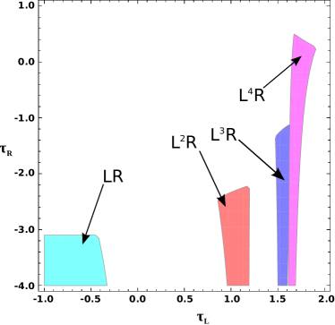
Figure 1: Regions of the projected parameter space where stable $L^{n}R$ orbits exist. The plot has been made by setting $\sigma_{L}=\sigma_{R}=1.4$, $\delta_{L}=\delta_{R}=0.7$ and $\mu=1$.

In three dimensions, the normal matrix (10) takes the form

$$M=\begin{pmatrix}\tau&1&0\\ -\sigma&0&1\\ \delta&0&0\end{pmatrix}.$$ (18)

Hence, by (16)

$$M^{n}=\begin{pmatrix}\Gamma_{1,n}&\Gamma_{1,n-1}&\Gamma_{1,n-2}\\ \Gamma_{2,n}&\Gamma_{2,n-1}&\Gamma_{2,n-2}\\ \Gamma_{3,n}&\Gamma_{3,n-1}&\Gamma_{3,n-2}\end{pmatrix}$$ (19)

where

$$\Gamma_{i,n}=\tau\Gamma_{i,n-1}-\sigma\Gamma_{i,n-2}+\delta\Gamma_{i,n-3}$$ (20)

for $i\in\left\{1,2,3\right\}$ and $n>1$. For $-1\leq n\leq 1$, the terms are taken from $M$ according to (14). Using these expressions, we compute the required powers of $M_{L}$ and $M_{R}$, and substitute them in (7) and (8) to obtain the required conditions for existence and stability of $L^{n}R$ orbits for various values of $n$. The parameter values for which the stable orbits exist are shown in Fig. 1 where the plausible regions are shown in the two dimensional projection of the six dimensional space.

Now let us consider the special case of 2 dimensions where further simplification can be done and the $n^{th}$ power of $M$ can be computed non-iteratively.

VI Computing $M^{n}$ for 2 Dimensions

In two dimensions the matrix appearing in the normal form map is given by (4). Dropping the subscripts for notational simplicity as in the previous section gives us

$$M=\begin{pmatrix}\tau&1\\ -\delta&0\end{pmatrix}.$$ (21)

From the results obtained in the previous section, it can be said that $M^{n}$ would be determined by two independent sequences $a$ and $b$ and would be of the form

$$M^{n}=\begin{pmatrix}a_{n}&a_{n-1}\\ b_{n}&b_{n-1}\end{pmatrix}.$$ (22)

However on explicit calculation (as done in Appendix B) it can be shown that the terms of the two sequences are related as

$$b_{i}=-\delta a_{i-1}~{}~{}~{}\forall i\geq 0.$$ (23)

Substituting (23) in (22) gives the final form of $M^{n}$ as

$$M^{n}=\begin{pmatrix}a_{n}&a_{n-1}\\ -\delta a_{n-1}&-\delta a_{n-2}\end{pmatrix}~{}~{}~{}\forall n\in\mathbb{N}$$ (24)

where

$$a_{n}=\tau a_{n-1}-\delta a_{n-2}~{}~{}~{}\forall i\in\mathbb{N}$$ (25)

with initial conditions $a_{0}=1$ and $a_{-1}=0$. Apart from the iterative definition, it is also possible to explicitly determine $a_{n}$ in terms of known quantities.

In terms of $\tau$ and $\delta$, $a_{n}$ is given as

$$a_{n}=\sum\limits_{m=0}^{\left[\dfrac{n}{2}\right]}\left(-1\right)^{m}~{}^{n-m}C_{m}~{}\delta^{m}~{}\tau^{n-2m}~{}~{}~{}\forall n\geq 0$$ (26)

and $a_{-1}=0$. Here $[\cdot]$ is the greatest integer function and $~{}^{n}C_{r}$ is the coefficient of $x^{r}$ in the binomial expansion of $(1+x)^{n}$. Using the properties of $~{}^{n}C_{r}$, it can be shown the $a_{n}$ as expressed in (26) satisfies (25). However as the proof is lengthy, it is given in Appendix C.

We can also obtain another representation of $a_{n}$ if the results are expressed in terms of the eigenvalues of $M$,

$$\lambda_{1,2}=\dfrac{\tau\pm\sqrt{\tau^{2}-4\delta}}{2}.$$ (27)

To do so, we put $\tau=\lambda_{1}+\lambda_{2}$ and $\delta=\lambda_{1}\lambda_{2}$ in (21). We then decompose $M$ as $M=UDU^{-1}$ where $D$ is the diagonal matrix with $\lambda_{1}$ and $\lambda_{2}$ on its diagonals and $U$ is the matrix with the eigenvectors of $M$ as the columns. Then $M^{n}=UD^{n}U^{-1}$, which when computed explicitly gives

$$M^{n}=\dfrac{1}{\lambda_{2}-\lambda_{1}}\begin{pmatrix}\lambda_{2}^{n+1}-\lambda_{1}^{n+1}&\lambda_{2}^{n}-\lambda_{1}^{n}\\ \lambda_{1}^{n+1}\lambda_{2}-\lambda_{2}^{n+1}\lambda_{1}&\lambda_{1}^{n}\lambda_{2}-\lambda_{2}^{n}\lambda_{1}\end{pmatrix}$$

which can be recast into the form of (24) with the definition of $a_{n}$ as

$$a_{n}=\dfrac{\lambda_{1}^{n+1}-\lambda_{2}^{n+1}}{\lambda_{1}-\lambda_{2}}.$$ (28)

The detailed proof of this result is given in the Appendix D. It can also be directly seen that (28) satisfies (25).

Hence in order to compute $M^{n}$ for a $2\times 2$ matrix in the form (21), we use (26) or (28) to get $a_{n}$, $a_{n-1}$, $a_{n-2}$ and form the matrix given in (24).

The form of the matrix $M^{n}$ in (24) may be substituted directly into (6) to obtain the sum of the GP as

$$\phi_{n}=\begin{pmatrix}f_{n}&f_{n-1}\\ -\delta f_{n-1}&1-\delta f_{n-2}\end{pmatrix}$$ (29)

where

$$f_{n}=\dfrac{1-a_{n}+\delta a_{n-1}}{1-\tau+\delta}.$$ (30)

The detailed proof of this result is given in Appendix E. Note that the proof is independent of the explicit form of $a_{n}$ and uses only the propagation rule (25).

VII Comments on Speed of the Algorithm

Although results in Section-5 demonstrate the use of the algorithm described in this article, the effectiveness of the proposed algorithm can be gauged better in higher dimensional systems where computation of existence and stability conditions becomes computationally intensive due to large orders of matrices involved. In this section, we show the efficiency of the proposed method against the traditional methods as the dimensions of the system increases. To do this we compare the times required by the proposed method to compute powers of the matrix $M_{L/R}$ for various dimensions against the times required by other frequently used methods for the same computation.

First let us look at the computational complexity of the proposed algorithm. As noted erlier, the efficiency of the proposed method lies in the structure of the matrices $M_{L/R}$. We note from (17) that

$$\left[M^{n}\right]_{i,j}=\Gamma_{i,n-(j-1)}=\Gamma_{i,(n+1)-((j+1)-1)}=\left[M^{n+1}\right]_{i,j+1}.$$ (31)

This implies that in $N$-dimensions, the first $N-1$ columns of $M^{n}$ is identical to the last $N-1$ columns of $M^{n+1}$. Hence, to compute $M^{n+1}$ from $M^{n}$, we need to compute only one new column of the matrix. The construction of this new column is described by (15). Computation of each term of the column requires $N$ multiplications. As there are $N$ elements in the row, the total number of multiplications to be performed to raise the $N$-dimensional matrix $M$ to the power $n$ is $N^{2}n$. Hence, the proposed algorithm has the computational complexity of the order $\mathcal{O}(N^{2}n)$.

Two of the most common methods for computing the powers of matrices are brute-force matrix multiplication and matrix diagonalisation. Brute-force matrix multiplication simply multiplies the matrices successively; hence making computation of $n^{th}$ power of an $N$-dimensional matrix an $\mathcal{O}(N^{3}n)$ process. On the other hand, matrix diagonalisation seeks to diagonalise the matrix $M$ as $M=UDU^{-1}$ and then compute the $n^{th}$ power as $M^{n}=UD^{n}U^{-1}$. While the method seems elegant, it involves diagonalisation of the matrix; making it an $\mathcal{O}(N^{3})$ process Arfken and Weber (2005). Even with more sophisticated matrix multiplications like Strassen algorithm Strassen (1969) or Coppersmith-Winograd algorithm Le Gall (2014); Davie and Stothers (2013); Coppersmith (1997), one obtains a order complexity of $\mathcal{O}(N^{q}n)$ with $q>2$. Comparing the order complexity of the proposed method (which is $\mathcal{O}(N^{2}n)$) with that of brute force matrix multiplication or matrix diagonalisation, we see that the proposed algorithm is better than the other methods at least for large enough matrix dimension.

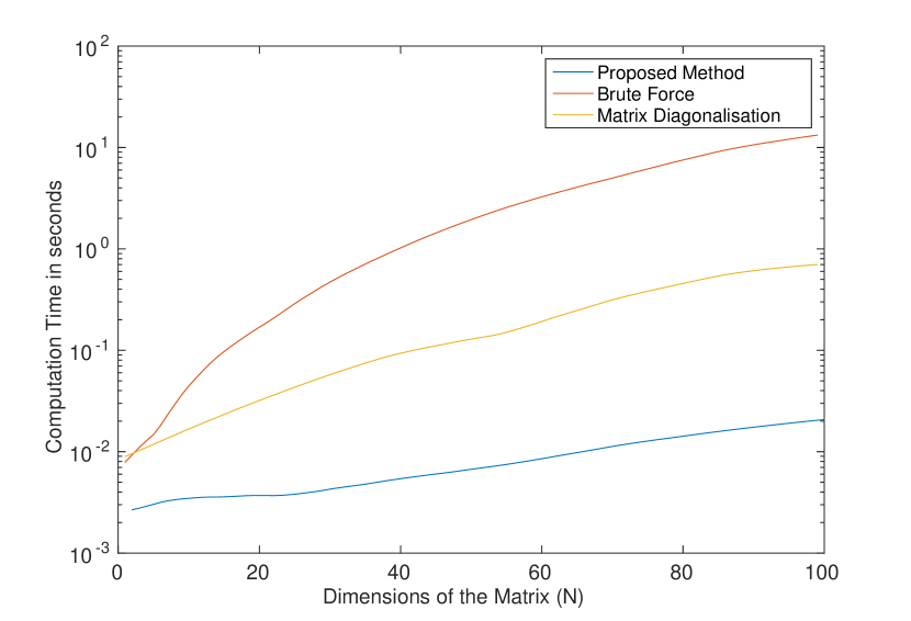
(a) Power computed, $m=10$

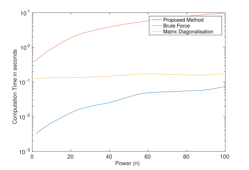
(b) Dimension of the Matrix, $N=50$

Figure 2: Comparison of the proposed algorithm of raising matrices to powers with the pre-existing methods. Plots show the time taken to perform 100 typical calculations by each of the algorithms. For each dimension and power, 1000 sets of 100 random matrices of the form (10) each were taken and the total time taken for computation was averaged over the 1000 sets.

However, to get an estimate for realistic dimensions and powers, we computed the powers of random matrices of the form (10) on a computer using the three algorithms: a) the proposed algorithm, b) matrix diagonalisation and c) brute force matrix multiplication to compare their run-times. Figure 2 shows the time taken by the different algorithms on the same computer to compute the powers of random matrices of the form (10). As can be evidently seen, the efficiency of the proposed method, when compared to the other algorithms increases with increase in the dimension of the matrices when the power to which the matrices are raised is kept constant. When the matrix power is increased keeping the dimension of the matrix fixed, we see that the gain provided by the proposed algorithm as compared to matrix diagonalisation reduces as $n$ is increased. However, the proposed algorithm performs better than matrix diagonalisation for a significantly large range of $n$. Only for very high powers of matrices is matrix diagonaisation a better algorithm than the proposed one.

Hence the proposed algorithm is seen to perform better than the competing algorithms for high dimensional systems when we are interested in sufficiently lower powers of the matrix. Physically, this corresponds to periodic orbits of sufficiently low periodicity in high dimensional phase space. Non-smooth dynamical systems with high dimensionality occur in many real-life electrical, electronic and robotic systems where the dimensions of the phase space can well go over 50 due the presence of many components. The proposed algorithm might hence be applied to such dynamical systems to increase computational efficiency.

VIII Conclusion

In this article we developed a faster and a more elegant technique to compute the existence and stability conditions for periodic orbits of the form $L^{m}R^{n}$ in an arbitrary dimensional piecewise linear continuous map. The technique is based on easier computation of powers of $N\times N$ matrices in their normal form. Due to the structure of the matrices involved, it was found that the elements of the resulting matrix were interrelated; and in order to compute the $n^{th}$ power of the matrix, only $N$ out of the $N^{2}$ elements need to be computed. These $N$ elements in turn can be obtained as simple sequences defined iteratively. Once the powers of the matrices are computed, they can be substituted in the generic expressions of existence and stability of orbits to obtain the regions in parameter space where they exist. We also apply the technique developed to 3 dimensional systems and obtain the regions where $L^{n}R$ orbits exist.

Moreover, in the special case of 2 dimensional matrices, further simplifications were made. Notably, explicit expressions for the terms of the sequence in terms of the given parameters and eigenvalues of the matrices were obtained. This allows for a direct evaluation of any power of the $2\times 2$ normal form matrix without computing the intermediate powers.

Appendix: Derivations and Motivations

Appendix A Finding $M^{n}$ for a Matrix $M$ in the Normal Form

Theorem A.1

Let $M$ a matrix of the form (10). Then the elements of $M^{n}$ are given as

$$\left[M^{n}\right]_{i,j}=\Gamma_{i,n-(j-1)}~{}~{}~{}\forall n\in\mathbb{N}$$ (32)

where $\left[A\right]_{i,j}$ is the element of $A$ corresponding to $i^{th}$ row and $j^{th}$ column and $\Gamma_{i,j}$ is defined in (13) and (15).

• Let us assume the most general form of $M^{n}$

  $$M^{n}=\begin{pmatrix}\theta^{(n)}_{1,1}&\cdots&\theta^{(n)}_{1,N}\\ \vdots&\ddots&\vdots\\ \theta^{(n)}_{N,1}&\cdots&\theta^{(n)}_{N,N}\\ \end{pmatrix}$$ (33)

  for some $n\geq 1$. Then

  $$M^{n+1} =\begin{pmatrix}\theta^{(n)}_{1,1}&\theta^{(n)}_{1,2}&\cdots&\theta^{(n)}_{1,N}\\ \theta^{(n)}_{2,1}&\theta^{(n)}_{2,2}&\cdots&\theta^{(n)}_{2,N}\\ \vdots&\vdots&\cdots&\vdots\\ \theta^{(n)}_{N,1}&\theta^{(n)}_{N,2}&\cdots&\theta^{(n)}_{N,N}\\ \end{pmatrix}\cdot\begin{pmatrix}\rho_{1}&1&\cdots&0\\ -\rho_{2}&0&\cdots&0\\ \vdots&\vdots&\cdots&\vdots\\ (-1)^{N-1}~{}\rho_{N}&0&\cdots&0\end{pmatrix}$$

  $$\begin{pmatrix}\theta^{(n+1)}_{1,1}&\theta^{(n+1)}_{1,2}&\cdots&\theta^{(n+1)}_{1,N}\\ \theta^{(n+1)}_{2,1}&\theta^{(n+1)}_{2,2}&\cdots&\theta^{(n+1)}_{2,N}\\ \vdots&\vdots&\cdots&\vdots\\ \theta^{(n+1)}_{N,1}&\theta^{(n+1)}_{N,2}&\cdots&\theta^{(n+1)}_{N,N}\\ \end{pmatrix} =\begin{pmatrix}\left(\sum_{k=1}^{N}(-1)^{k-1}\rho_{k}\theta^{(n)}_{1,k}\right)&\theta^{(n)}_{1,1}&\cdots&\theta^{(n)}_{1,N-1}\\ \left(\sum_{k=1}^{N}(-1)^{k-1}\rho_{k}\theta^{(n)}_{2,k}\right)&\theta^{(n)}_{2,1}&\cdots&\theta^{(n)}_{2,N-1}\\ \vdots&\vdots&\cdots&\vdots\\ \left(\sum_{k=1}^{N}(-1)^{k-1}\rho_{k}\theta^{(n)}_{N,k}\right)&\theta^{(n)}_{N,1}&\cdots&\theta^{(n)}_{N,N-1}\end{pmatrix}$$

  Hence

  $$\theta^{(n+1)}_{i,1}=\sum_{k=1}^{N}(-1)^{k-1}\rho_{k}\theta^{(n)}_{i,k}~{}~{}~{}:1\leq i\leq N,n\geq 1$$ (34)

  and

  $$\theta^{(n+1)}_{i,j}=\theta^{(n)}_{i,j-1}~{}~{}~{}:1\leq i\leq N,~{}1<j\leq N,n\geq 1.$$ (35)

  We now use (35) iteratively to obtain

  $$\theta^{(n+1)}_{i,j}=\theta^{(n)}_{i,j-1}=\theta^{(n-1)}_{i,j-2}=\ldots=\theta^{(n-(j-2))}_{i,1}~{}~{}~{}:1\leq i\leq N,~{}1<j\leq N,n\geq 1.$$ (36)

  Now if we define

  $$\theta^{(n+1)}_{i,1}=\Gamma_{i,n+1}~{}~{}~{}:1\leq i\leq N$$ (37)

  then

  $$\theta^{(n+1)}_{i,j}=\theta^{(n-(j-2))}_{i,1}=\Gamma_{i,n-(j-2)}~{}~{}~{}:1\leq i\leq N,~{}1<j\leq N,n\geq 1.$$ (38)

  Combining (37) and (38); and replacing $n+1$ by $n$ we get

  $$\theta^{(n)}_{i,j}=\Gamma_{i,n-(j-1)}~{}~{}~{}:1\leq i,j\leq N,n\geq 2.$$ (39)

  Now, by definition

  $$\Gamma_{i,n+1}=\theta^{(n+1)}_{i,1}=\sum_{k=1}^{N}(-1)^{k-1}\rho_{k}\theta^{(n)}_{i,k}~{}~{}~{}:1\leq i\leq N,n\geq 1.$$ (40)

  Using (39) in the right hand side gives us

  $$\Gamma_{i,n+1}=\theta^{(n+1)}_{i,1}=\sum_{k=1}^{N}(-1)^{k-1}\rho_{k}\Gamma_{i,n-(k-1)}~{}~{}~{}:1\leq i\leq N,n\geq 1.$$ (41)

  Finally replacing $n+1$ by $j$, we have an iterative relation for $\Gamma_{i,j}$ as

  $$\Gamma_{i,j}=\sum_{k=1}^{N}(-1)^{k-1}\rho_{k}\Gamma_{i,j-k}~{}~{}~{}:1\leq i\leq N,j\geq 2.$$ (42)

  Now note that substituting $n=1$ in (39) gives

  $$\theta^{(1)}_{i,j}=\Gamma_{i,2-j}~{}~{}~{}:1\leq i,j\leq N.$$ (43)

  However by definition of $\theta^{(n)}_{i,j}$, we have

  $$\theta^{(1)}_{i,j}=\left[M^{1}\right]_{i,j}=M_{i,j}~{}~{}~{}:1\leq i,j\leq N.$$ (44)

  Hence,

  $$\Gamma_{i,2-j}=M_{i,j}~{}~{}~{}:1\leq i,j\leq N$$ (45)

  which on replacing $2-j$ by $j$ yields

  $$\Gamma_{i,j}=M_{i,2-j}~{}~{}~{}:1\leq i\leq N,-N+2\leq j\leq 1$$ (46)

Appendix B Motivating the Form of $a_{n}$

In this Appendix, we give the motivation for obtaining the fundamental sequence in the form

$$a_{n}=\sum\limits_{m=0}^{\left[\frac{n}{2}\right]}\left(-1\right)^{m}~{}^{n-m}C_{m}~{}\delta^{m}~{}\tau^{n-2m}~{}~{}~{}\forall n\geq 0$$ (47)

and $a_{-1}=0$. In other terms, we try to understand, how the matrix

$$M=\begin{pmatrix}\tau&1\\ -\delta&0\end{pmatrix}.$$ (48)

yields

$$M^{n}=\begin{pmatrix}a_{n}&a_{n-1}\\ -\delta a_{n-1}&-\delta a_{n-2}\end{pmatrix}~{}~{}~{}\forall n\in\mathbb{N}$$ (49)

with $a_{n}$ defined in (47).

For an matrix general $2\times 2$ matrix $M$, if we assume

$$M^{n}=\begin{pmatrix}a_{n}&b_{n}\\ c_{n}&d_{n}\end{pmatrix}$$ (50)

then the sequence

$$M,M^{2},M^{3},\ldots,M^{n}$$ (51)

or

$$\begin{pmatrix}a_{1}&b_{1}\\ c_{1}&d_{1}\end{pmatrix},\begin{pmatrix}a_{2}&b_{2}\\ c_{2}&d_{2}\end{pmatrix},\begin{pmatrix}a_{3}&b_{3}\\ c_{3}&d_{3}\end{pmatrix},\ldots,\begin{pmatrix}a_{n}&b_{n}\\ c_{n}&d_{n}\end{pmatrix}$$ (52)

is a set of four sequences: $\left\{a_{n}\right\},\left\{b_{n}\right\},\left\{c_{n}\right\}$ and $\left\{d_{n}\right\}$.

The aim of the section is to show that these four sequences are restricted by constraints that allow the matrix to be expressed in terms of a single sequence.

To show this, we assume that (50) holds for the matrix defined in (48). Then

$$M^{n+1} =M^{n}.M$$

$$\begin{pmatrix}a_{n+1}&b_{n+1}\\ c_{n+1}&d_{n+1}\end{pmatrix} =\begin{pmatrix}a_{n}&b_{n}\\ c_{n}&d_{n}\end{pmatrix}\begin{pmatrix}\tau&1\\ -\delta&0\end{pmatrix}$$

$$\begin{pmatrix}a_{n+1}&b_{n+1}\\ c_{n+1}&d_{n+1}\end{pmatrix} =\begin{pmatrix}\tau a_{n}-\delta b_{n}&a_{n}\\ \tau c_{n}-\delta d_{n}&c_{n}\end{pmatrix}$$

Hence

$$b_{n+1} =a_{n}$$

$$d_{n+1} =c_{n}$$

or

$$b_{n}=a_{n-1}$$ (53)

$$d_{n}=c_{n-1}$$ (54)

and

$$a_{n+1}=\tau a_{n}-\delta b_{n}$$ (55)

$$c_{n+1}=\tau c_{n}-\delta d_{n}.$$ (56)

Substituting (53) in (55) and (54) in (56), we get

$$a_{n+1}=\tau a_{n}-\delta a_{n-1}$$ (57)

$$c_{n+1}=\tau c_{n}-\delta c_{n-1}.$$ (58)

Hence, at the current stage

$$M^{n}=\begin{pmatrix}a_{n}&a_{n-1}\\ c_{n}&c_{n-1}\end{pmatrix}$$ (59)

with $a_{n}$ and $c_{n}$ satisfying (57) and (58) respectively.

Moreover, as we know

$$M^{1}=\begin{pmatrix}a_{1}&a_{0}\\ c_{1}&c_{0}\end{pmatrix}=M=\begin{pmatrix}\tau&1\\ -\delta&0\end{pmatrix},$$

therefore

$$a_{1}=\tau,~{}a_{0}=1,~{}c_{1}=-\delta,~{}c_{0}=0.$$ (60)

Using (57) and (58) in conjugation with the initial conditions in (60), can write the complete sequence of $a_{n}$ and $c_{n}$. The first few terms are shown below.

$$a_{1} =\tau$$

$$a_{2} =\tau^{2}-\delta$$

$$a_{3} =\tau^{3}-2\tau\delta$$

$$a_{4} =\tau^{4}-3\tau^{2}\delta+\delta^{2}$$

$$a_{5} =\tau^{5}-4\tau^{3}\delta+3\tau\delta^{2}$$

$$a_{6} =\tau^{6}-5\tau^{4}\delta+6\tau^{2}\delta^{2}-\delta^{3}$$

$$a_{7} =\tau^{7}-6\tau^{5}\delta+10\tau^{3}\delta^{2}-4\tau\delta^{3}$$

$$a_{8} =\tau^{8}-7\tau^{6}\delta+15\tau^{4}\delta^{2}-10\tau^{2}\delta^{3}+\delta^{4}$$

$$a_{9} =\tau^{9}-8\tau^{7}\delta+21\tau^{5}\delta^{2}-20\tau^{3}\delta^{3}+5\tau\delta^{4}$$

$$c_{1} =-\delta$$

$$c_{2} =-\delta[\tau]$$

$$c_{3} =-\delta[\tau^{2}-\delta]$$

$$c_{4} =-\delta[\tau^{3}-2\tau\delta]$$

$$c_{5} =-\delta[\tau^{4}-3\tau^{2}\delta+\delta^{2}]$$

$$c_{6} =-\delta[\tau^{5}-4\tau^{3}\delta+3\tau\delta^{2}]$$

$$c_{7} =-\delta[\tau^{6}-5\tau^{4}\delta+6\tau^{2}\delta^{2}-\delta^{3}]$$

$$c_{8} =-\delta[\tau^{7}-6\tau^{5}\delta+10\tau^{3}\delta^{2}-4\tau\delta^{3}]$$

$$c_{9} =-\delta[\tau^{8}-7\tau^{6}\delta+15\tau^{4}\delta^{2}-10\tau^{2}\delta^{3}+\delta^{4}]$$

It may be noted that if written in the appropriate form, it becomes clear that

$$c_{n}=-\delta a_{n}~{}~{}~{}\forall n\in\mathbb{N}.$$ (61)

In order to extend the result to $c_{0}$, we define $a_{-1}=0$ which allows us to write $M^{n}$ as

$$M^{n}=\begin{pmatrix}a_{n}&a_{n-1}\\ -\delta a_{n-1}&-\delta a_{n-2}\end{pmatrix}$$ (62)

where

$$a_{n+1}=\tau a_{n}-\delta a_{n-1}~{}~{}~{}\forall n\geq 0$$ (63)

and $a_{-1}=0$.

To obtain the analytic expression for $a_{n}$, we note the following in expansions given earlier. when terms under summation for a particular $n$ value are arranged in the ascending order of powers of $\delta$,

• There are $\left[\frac{n}{2}\right]+1$ terms in the series.

• Powers of $\delta$ start from $0$ and increase in steps of 1.

• Powers of $\tau$ start from $n$ and decrease in steps of 2.

• Sign of each term alternates between plus and minus starting from a plus

• A numerical coefficient precedes each term.

Hence $a_{n}$ can be written as

$$a_{n}=\sum_{m=0}^{\left[\frac{n}{2}\right]}\left(-1\right)^{m}~{}\eta_{m,n}~{}\delta^{m}\tau^{n-2m}$$ (64)

Table 1: List of all $\eta_{m,n}$ values

$\eta_{m,n}$	0	1	2	3	4
1	1
2	1	1
3	1	2
4	1	3	1
5	1	4	3
6	1	5	6	1
7	1	6	10	4
8	1	7	15	10	1
9	1	8	21	20	5

A look at the $\eta_{m,n}$ values in Table 1 reveal that

$$\eta_{m,n}=\eta_{m,n-1}+\eta_{m-1,n-2}$$ (65)

which seems similar to the properties of the binomial coefficients. In fact,

$$\eta_{m,n}=~{}^{n-m}C_{m}~{}$$ (66)

and the structure of the Pascal’s triangle might be evidently seen in the table.

Appendix C The Progression Rule of Fundamental Sequence

Lemma C.1

The $n^{th}$ term of the sequence defined in (26) is related to its two preceding terms by the relation

$$a_{n}=\tau a_{n-1}-\delta a_{n-2}.$$ (67)

• For $n=0$,

  $$a_{n+1} =a_{1}=\tau$$

  $$a_{n} =a_{0}=1$$

  $$a_{n-1} =a_{-1}=0$$

  Hence (67) is true for $n=0$.

  For the other $n$, we prove it separately for even and odd $n$.

  If $n$ is even, then

  $$\left[\dfrac{n}{2}\right]=\dfrac{n}{2},~{}~{}~{}\left[\dfrac{n-1}{2}\right]=\dfrac{n}{2}-1,~{}~{}~{}\left[\dfrac{n+1}{2}\right]=\dfrac{n}{2}.$$ (68)

  Now,

  $$\tau a_{n}-\delta a_{n-1} =\tau\sum_{m=0}^{\left[\dfrac{n}{2}\right]}\left((-1)^{m}~{}^{n-m}C_{m}~{}\delta^{m}\tau^{n-2m}\right)-\delta\sum_{m=0}^{\left[\dfrac{n-1}{2}\right]}\left((-1)^{m}~{}^{n-1-m}C_{m}~{}\delta^{m}\tau^{n-1-2m}\right)$$

  $$=\sum_{m=0}^{\dfrac{n}{2}}\left((-1)^{m}~{}^{n-m}C_{m}~{}\delta^{m}\tau^{n+1-2m}\right)-\sum_{m=0}^{\dfrac{n}{2}-1}\left((-1)^{m}~{}^{n-1-m}C_{m}~{}\delta^{m+1}\tau^{n-1-2m}\right)$$

  $$=\tau^{n+1}+\sum_{m=1}^{\dfrac{n}{2}}\left((-1)^{m}~{}^{n-m}C_{m}~{}\delta^{m}\tau^{n+1-2m}\right)-\sum_{m=0}^{\dfrac{n}{2}-1}\left((-1)^{m}~{}^{n-1-m}C_{m}~{}\delta^{m+1}\tau^{n-1-2m}\right)$$

  $$=\tau^{n+1}+\sum_{m=1}^{\dfrac{n}{2}}\left((-1)^{m}~{}^{n-m}C_{m}~{}\delta^{m}\tau^{n+1-2m}\right)+\sum_{m=1}^{\dfrac{n}{2}}\left((-1)^{m}~{}^{n-m}C_{m-1}~{}\delta^{m}\tau^{n+1-2m}\right)$$

  $$=\tau^{n+1}+\sum_{m=1}^{\dfrac{n}{2}}\left((-1)^{m}\left(~{}^{n-m}C_{m}~{}+~{}^{n-m}C_{m-1}~{}\right)\delta^{m}\tau^{n+1-2m}\right)$$

  $$=\tau^{n+1}+\sum_{m=1}^{\dfrac{n}{2}}\left((-1)^{m}~{}^{n+1-m}C_{m}~{}\delta^{m}\tau^{n+1-2m}\right)$$

  $$=\sum_{m=0}^{\left[\dfrac{n+1}{2}\right]}\left((-1)^{m}~{}^{n+1-m}C_{m}~{}\delta^{m}\tau^{n+1-2m}\right)$$

  $$=a_{n+1}.$$

  If $n$ is odd then

  $$\left[\frac{n}{2}\right]=\frac{n-1}{2},~{}~{}~{}\left[\frac{n-1}{2}\right]=\frac{n-1}{2},~{}~{}~{}\left[\frac{n+1}{2}\right]=\frac{n+1}{2}.$$ (69)

  Now,

  $$\tau a_{n}-\delta a_{n-1} =\tau\sum_{m=0}^{\left[\frac{n}{2}\right]}\left((-1)^{m}~{}^{n-m}C_{m}~{}\delta^{m}\tau^{n-2m}\right)-\delta\sum_{m=0}^{\left[\frac{n-1}{2}\right]}\left((-1)^{m}~{}^{n-1-m}C_{m}~{}\delta^{m}\tau^{n-1-2m}\right)$$

  $$=\sum_{m=0}^{\frac{n-1}{2}}\left((-1)^{m}~{}^{n-m}C_{m}~{}\delta^{m}\tau^{n+1-2m}\right)-\sum_{m=0}^{\frac{n-1}{2}-1}\left((-1)^{m}~{}^{n-1-m}C_{m}~{}\delta^{m+1}\tau^{n-1-2m}\right)$$

  $$=\tau^{n+1}+\sum_{m=1}^{\frac{n-1}{2}}\left((-1)^{m}~{}^{n-m}C_{m}~{}\delta^{m}\tau^{n+1-2m}\right)-\sum_{m=0}^{\frac{n-3}{2}}\left((-1)^{m}~{}^{n-1-m}C_{m}~{}\delta^{m+1}\tau^{n-1-2m}\right)-(-1)^{\frac{n-1}{2}}\delta^{\frac{n+1}{2}}$$

  $$=\tau^{n+1}+\sum_{m=1}^{\frac{n-1}{2}}\left((-1)^{m}~{}^{n-m}C_{m}~{}\delta^{m}\tau^{n+1-2m}\right)+\sum_{m=1}^{\frac{n-1}{2}}\left((-1)^{m}~{}^{n-m}C_{m-1}~{}\delta^{m}\tau^{n+1-2m}\right)+(-1)^{\frac{n+1}{2}}\delta^{\frac{n+1}{2}}$$

  $$=\tau^{n+1}+\sum_{m=1}^{\frac{n-1}{2}}\left((-1)^{m}\left(~{}^{n-m}C_{m}~{}+~{}^{n-m}C_{m-1}~{}\right)\delta^{m}\tau^{n+1-2m}\right)+(-1)^{\frac{n+1}{2}}\delta^{\frac{n+1}{2}}$$

  $$=\tau^{n+1}+\sum_{m=1}^{\frac{n-1}{2}}\left((-1)^{m}~{}^{n+1-m}C_{m}~{}\delta^{m}\tau^{n+1-2m}\right)+(-1)^{\frac{n+1}{2}}\delta^{\frac{n+1}{2}}$$

  $$=\sum_{m=0}^{\left[\frac{n+1}{2}\right]}\left((-1)^{m}~{}^{n+1-m}C_{m}~{}\delta^{m}\tau^{n+1-2m}\right)$$

  $$=a_{n+1}.$$

  Hence the result is true for all $n\in\mathbb{N}$.

Appendix D $M^{n}$ in Terms of Eigenvalues

Theorem D.1

Let

$$M=\begin{pmatrix}\tau&1\\ -\delta&0\end{pmatrix}$$ (70)

with the eigenvalues

$$\lambda_{1,2}=\frac{\tau\pm\sqrt{\tau^{2}-4\delta}}{2}$$ (71)

then

$$M^{n}=\begin{pmatrix}a_{n}&a_{n-1}\\ -\delta a_{n-1}&-\delta a_{n-2}\end{pmatrix}~{}~{}~{}\forall n\in\mathbb{N}$$ (72)

where

$$a_{n}=\frac{\lambda_{1}^{n+1}-\lambda_{2}^{n+1}}{\lambda_{1}-\lambda_{2}}.$$ (73)

• Let $\lambda_{1}$ and $\lambda_{2}$ be the eigenvectors of $M$. Substituting the trace $\tau=\lambda_{1}+\lambda_{2}$ and determinant $\delta=\lambda_{1}\lambda_{2}$, we have

  $$M=\begin{pmatrix}\lambda_{1}+\lambda_{2}&1\\ -\lambda_{1}\lambda_{2}&0\end{pmatrix}.$$ (74)

  Simple calculation of shows that the eigenvector corresponding to $\lambda_{1}$ is $\begin{pmatrix}1\\ -\lambda_{2}\end{pmatrix}$ and that corresponding to $\lambda_{2}$ is $\begin{pmatrix}1\\ -\lambda_{1}\end{pmatrix}$. Hence, we may construct a matrix $U$ with eigenvectors as columns,

  $$U=\begin{pmatrix}1&1\\ -\lambda_{2}&-\lambda_{1}\end{pmatrix}$$ (75)

  and a diagonal matrix $D$ with the eigenvalues

  $$D=\begin{pmatrix}\lambda_{1}&0\\ 0&\lambda_{2}\end{pmatrix}$$ (76)

  such that

  $$M=UDU^{-1}.$$ (77)

  and hence

  $$M^{n}=UD^{n}U^{-1}.$$ (78)

  Substituting the values, we get

  $$M^{n} =\begin{pmatrix}1&1\\ -\lambda_{2}&-\lambda_{1}\end{pmatrix}\begin{pmatrix}\lambda_{1}&0\\ 0&\lambda_{2}\end{pmatrix}^{n}\begin{pmatrix}1&1\\ -\lambda_{2}&-\lambda_{1}\end{pmatrix}^{-1}$$

  $$=\frac{1}{\lambda_{2}-\lambda_{1}}\begin{pmatrix}1&1\\ -\lambda_{2}&-\lambda_{1}\end{pmatrix}\begin{pmatrix}\lambda_{1}^{n}&0\\ 0&\lambda_{2}^{n}\end{pmatrix}\begin{pmatrix}-\lambda_{1}&-1\\ \lambda_{2}&1\end{pmatrix}$$

  $$=\frac{1}{\lambda_{2}-\lambda_{1}}\begin{pmatrix}1&1\\ -\lambda_{2}&-\lambda_{1}\end{pmatrix}\begin{pmatrix}-\lambda_{1}^{n+1}&-\lambda_{2}^{n}\\ \lambda_{2}^{n+1}&\lambda_{2}^{n}\end{pmatrix}$$

  $$=\frac{1}{\lambda_{2}-\lambda_{1}}\begin{pmatrix}\lambda_{2}^{n+1}-\lambda_{1}^{n+1}&\lambda_{2}^{n}-\lambda_{1}^{n}\\ \lambda_{1}^{n+1}\lambda_{2}-\lambda_{2}^{n+1}\lambda_{1}&\lambda_{1}^{n}\lambda_{2}-\lambda_{2}^{n}\lambda_{1}\end{pmatrix}$$

  which can be recast as

  $$M^{n}=\begin{pmatrix}a_{n}&a_{n-1}\\ -\delta a_{n-1}&-\delta a_{n-2}\end{pmatrix}$$ (79)

  with

  $$a_{n}=\frac{\lambda_{1}^{n+1}-\lambda_{2}^{n+1}}{\lambda_{1}-\lambda_{2}}.$$ (80)

Appendix E The Form of $\phi_{n}$

Corollary E.1

The sum of the geometric progression

$$\phi_{n}=I+M+M^{2}+\ldots+M^{n}$$

is given as

$$\phi_{n}=\begin{pmatrix}f_{n}&f_{n-1}\\ -\delta f_{n-1}&1-\delta f_{n-2}\end{pmatrix}$$ (81)

where

$$f_{n}=\frac{1-a_{n}+\delta a_{n-1}}{1-\tau+\delta}.$$ (82)

• Using the formula for sum of GP, we can write $\phi_{n}$ as

  $$\phi_{n}=\frac{I-M^{n}}{I-M}.$$ (83)

  Hence

  $$\phi_{n} =\left[\begin{pmatrix}1&0\\ 0&1\end{pmatrix}-\begin{pmatrix}\tau&1\\ -\delta&0\end{pmatrix}\right]^{-1}\left[\begin{pmatrix}1&0\\ 0&1\end{pmatrix}-\begin{pmatrix}a_{n}&a_{n-1}\\ -\delta a_{n-1}&-\delta a_{n-2}\end{pmatrix}\right]$$

  $$=\begin{pmatrix}1-\tau&-1\\ \delta&1\end{pmatrix}^{-1}\begin{pmatrix}1-a_{n}&-a_{n-1}\\ \delta a_{n-1}&1+\delta a_{n-2}\end{pmatrix}$$

  $$=\frac{1}{1-\tau+\delta}\begin{pmatrix}1&1\\ -\delta&1-\tau\end{pmatrix}\begin{pmatrix}1-a_{n}&-a_{n-1}\\ \delta a_{n-1}&1+\delta a_{n-2}\end{pmatrix}$$

  $$=\frac{1}{1-\tau+\delta}\begin{pmatrix}1-a_{n}+\delta a_{n-1}&1-a_{n-1}+\delta a_{n-2}\\ -\delta\left(1-a_{n}\right)+\delta a_{n-1}\left(1-\tau\right)&\delta a_{n-1}+\left(1-\tau\right)\left(1+\delta a_{n-2}\right)\end{pmatrix}$$

  $$=\begin{pmatrix}\frac{1-a_{n}+\delta a_{n-1}}{1-\tau+\delta}&\frac{1-a_{n-1}+\delta a_{n-2}}{1-\tau+\delta}\\ \frac{-\delta\left(1-a_{n}\right)+\delta a_{n-1}\left(1-\tau\right)}{1-\tau+\delta}&\frac{\delta a_{n-1}+\left(1-\tau\right)\left(1+\delta a_{n-2}\right)}{1-\tau+\delta}\end{pmatrix}$$

  Currently, $\phi_{n}$ is of the form

  $$\phi_{n}=\begin{pmatrix}f_{n}&f_{n-1}\\ \sigma_{1}&\sigma_{2}\end{pmatrix}$$ (84)

  with

  $$\sigma_{1}=\frac{-\delta\left(1-a_{n}\right)+\delta a_{n-1}\left(1-\tau\right)}{1-\tau+\delta}$$ (85)

  and

  $$\sigma_{2}=\frac{\delta a_{n-1}+\left(1-\tau\right)\left(1+\delta a_{n-2}\right)}{1-\tau+\delta}.$$ (86)

  Using lemma 67, we simplify $\sigma_{1}$ and $\sigma_{2}$ as

  $$\sigma_{1} =\frac{-\delta\left(1-a_{n}\right)+\delta a_{n-1}\left(1-\tau\right)}{1-\tau+\delta}$$

  $$=\frac{-\delta+\delta a_{n}+\delta a_{n-1}-\delta\tau a_{n-1}}{1-\tau+\delta}$$

  $$=\frac{-\delta\left(1-a_{n}-a_{n-1}+\tau a_{n-1}\right)}{1-\tau+\delta}$$

  $$=\frac{-\delta\left(1-a_{n}-a_{n-1}+a_{n}+\delta a_{n-2}\right)}{1-\tau+\delta}$$

  $$=\frac{-\delta\left(1-a_{n-1}+\delta a_{n-2}\right)}{1-\tau+\delta}$$

  $$=-\delta f_{n-1}.$$

  And

  $$\sigma_{2} =\frac{\delta a_{n-1}+\left(1-\tau\right)\left(1+\delta a_{n-2}\right)}{1-\tau+\delta}$$

  $$=\frac{\delta a_{n-1}+1+\delta a_{n-2}-\tau-\tau\delta a_{n-2}}{1-\tau+\delta}$$

  $$=\frac{1-\tau+\delta\left(a_{n-1}+a_{n-2}-\tau a_{n-2}\right)}{1-\tau+\delta}$$

  $$=\frac{1-\tau+\delta\left(a_{n-1}-\delta a_{n-3}\right)}{1-\tau+\delta}$$

  $$=\frac{1-\tau+\delta\left(-1+1+a_{n-1}-\delta a_{n-3}\right)}{1-\tau+\delta}$$

  $$=\frac{1-\tau+\delta+\delta\left(-1+a_{n-1}-\delta a_{n-3}\right)}{1-\tau+\delta}$$

  $$=\frac{1-\tau+\delta-\delta\left(1-a_{n-1}+\delta a_{n-3}\right)}{1-\tau+\delta}$$

  $$=1-\frac{\delta\left(1-a_{n-1}+\delta a_{n-3}\right)}{1-\tau+\delta}$$

  $$=1-\delta f_{n-2}.$$

  Therefore,

  $$\phi_{n}=\begin{pmatrix}f_{n}&f_{n-1}\\ -\delta f_{n-1}&1-\delta f_{n-2}\end{pmatrix}.$$ (87)

References

• Deaneย andย Hamill (1990) J.ย H.ย Deaneย andย D.ย C.ย Hamill,ย Power Electronics, IEEE Transactions onย 5,ย 260 (1990).
• Kousakaย etย al. (1999) T.ย Kousaka, T.ย Ueta, ย andย H.ย Kawakami,ย Circuits and Systems II: Analog and Digital Signal Processing, IEEE Transactions onย 46,ย 878 (1999).
• Nordmark (1991) A.ย B.ย Nordmark,ย Journal of Sound and Vibrationย 145,ย 279 (1991).
• Thuilotย etย al. (1997) B.ย Thuilot, A.ย Goswami, ย andย B.ย Espiau,ย inย Robotics and Automation, 1997. Proceedings., 1997 IEEE International Conference on,ย Vol.ย 1ย (IEEE,ย 1997)ย pp.ย 792โ€“798.
• Garciaย etย al. (1998) M.ย Garcia, A.ย Chatterjee, A.ย Ruina, ย andย M.ย Coleman,ย Journal of biomechanical engineeringย 120,ย 281 (1998).
• Sunย etย al. (1995) J.ย Sun, F.ย Amellal, L.ย Glass, ย andย J.ย Billette,ย Journal of theoretical biologyย 173,ย 79 (1995).
• Bรถrgersย andย Kopell (2003) C.ย Bรถrgersย andย N.ย Kopell,ย Neural computationย 15,ย 509 (2003).
• Banerjeeย etย al. (1998) S.ย Banerjee, J.ย A.ย Yorke, ย andย C.ย Grebogi,ย Physical Review Lettersย 80,ย 3049 (1998).
• Simpson (2014) D.ย J.ย Simpson,ย International Journal of Bifurcation and Chaosย 24 (2014).
• Nusseย andย Yorke (1992) H.ย E.ย Nusseย andย J.ย A.ย Yorke,ย Physica D: Nonlinear Phenomenaย 57,ย 39 (1992).
• Royย andย Roy (2008) I.ย Royย andย A.ย Roy,ย International Journal of Bifurcation and Chaosย 18,ย 577 (2008).
• Avrutinย etย al. (2012) V.ย Avrutin, M.ย Schanz, ย andย S.ย Banerjee,ย Nonlinear Dynamicsย 67,ย 293 (2012).
• Gardiniย etย al. (2010) L.ย Gardini, F.ย Tramontana, V.ย Avrutin, ย andย M.ย Schanz,ย International Journal of Bifurcation and Chaosย 20,ย 3085 (2010).
• Ganguliย andย Banerjee (2005) A.ย Ganguliย andย S.ย Banerjee,ย Physical Review Eย 71,ย 057202_1 (2005).
• Panchukย etย al. (2015) A.ย Panchuk, I.ย Sushko, ย andย V.ย Avrutin,ย International Journal of Bifurcation and Chaosย 25 (2015).
• Leonov (1959) N.ย Leonov,ย Radiofisicaย 3,ย 942 (1959).
• Leonov (1962) N.ย Leonov,ย Doklady Akademii Nauk SSSRย 143,ย 1038 (1962).
• Avrutinย etย al. (2010) V.ย Avrutin, M.ย Schanz, ย andย L.ย Gardini,ย Regular and Chaotic Dynamicsย 15,ย 685 (2010).
• Tramontanaย etย al. (2012) F.ย Tramontana, L.ย Gardini, V.ย Avrutin, ย andย M.ย Schanz,ย International Journal of Bifurcation and Chaosย 22 (2012).
• diย Bernardo (2003) M.ย diย Bernardo,ย inย Circuits and Systems, 2003. ISCASโ€™03. Proceedings of the 2003 International Symposium on,ย Vol.ย 3ย (IEEE,ย 2003)ย pp.ย IIIโ€“76.
• Arfkenย andย Weber (2005) G.ย B.ย Arfkenย andย H.ย J.ย Weber,ย Mathematical Methods For Physicists International Student Editionย (Academic press,ย 2005).
• Strassen (1969) V.ย Strassen,ย Numerische Mathematikย 13,ย 354 (1969).
• Leย Gall (2014) F.ย Leย Gall,ย inย Proceedings of the 39th international symposium on symbolic and algebraic computationย (ACM,ย 2014)ย pp.ย 296โ€“303.
• Davieย andย Stothers (2013) A.ย M.ย Davieย andย A.ย J.ย Stothers,ย Proceedings of the Royal Society of Edinburgh: Section A Mathematicsย 143,ย 351 (2013).
• Coppersmith (1997) D.ย Coppersmith,ย Journal of Complexityย 13,ย 42 (1997).