The Metropolis–Hastings algorithm

Abstract

This article is a self-contained introduction to the Metropolis-Hastings algorithm, this ubiquitous tool for producing dependent simulations from an arbitrary distribution. The document illustrates the principles of the methodology on simple examples with R codes and provides entries to the recent extensions of the method.

1 Introduction

There are many reasons why computing an integral like

$$\mathfrak{I}(h)=\int_{\mathcal{X}}h(x)\text{d}\pi(x),$$

where $\text{d}\pi$ is a probability measure, may prove intractable, from the shape of the domain $\mathcal{X}$ to the dimension of $\mathcal{X}$ (and $x$), to the complexity of one of the functions $h$ or $\pi$. Standard numerical methods may be hindered by the same reasons. Similar difficulties (may) occur when attempting to find the extrema of $\pi$ over the domain $\mathcal{X}$. This is why the recourse to Monte Carlo methods may prove unavoidable: exploiting the probabilistic nature of $\pi$ and its weighting of the domain $\mathcal{X}$ is often the most natural and most efficient way to produce approximations to integrals connected with $\pi$ and to determine the regions of the domain $\mathcal{X}$ that are more heavily weighted by $\pi$. The Monte Carlo approach (Hammersley and Handscomb, 1964; Rubinstein, 1981) emerged with computers, at the end of WWII, as it relies on the ability of producing a large number of realisations of a random variable distributed according to a given distribution, taking advantage of the stabilisation of the empirical average predicted by the Law of Large Numbers. However, producing simulations from a specific distribution may prove near impossible or quite costly and therefore the (standard) Monte Carlo may also face intractable situations.

An indirect approach to the simulation of complex distributions and in particular to the curse of dimensionality met by regular Monte Carlo methods is to use a Markov chain associated with this target distribution, using Markov chain theory to validate the convergence of the chain to the distribution of interest and the stabilisation of empirical averages (Meyn and Tweedie, 1994). It is thus little surprise that Markov chain Monte Carlo (MCMC) methods have been used for almost as long as the original Monte Carlo techniques, even though their impact on Statistics has not been truly felt until the very early 1990s. A comprehensive entry about the history of MCMC methods can be found in Robert and Casella (2010).

The paper is organised as follows: in Section 2, we define and justify the Metropolis–Hastings algorithm, along historical notes about its origin. In Section 3, we provide details on the implementation and calibration of the algorithm. A mixture example is processed in Section 4. Section 5 includes recent extensions of the standard Metropolis–Hastings algorithm, while Section 6 concludes about further directions for Markov chain Monte Carlo methods when faced with complex models and huge datasets.

2 The algorithm

2.1 Motivations

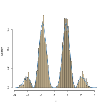
Figure 1: Fit of the histogram of a Metropolis–Hastings sample to its target, for $T=10^{4}$ iterations, a scale $\alpha=1$, and a starting value $x^{(1)}=3.14$.

Given a probability density $\pi$ called the target, defined on a state space $\mathcal{X}$, and computable up to a multiplying constant, $\pi(x)\propto\tilde{\pi}(x)$, the Metropolis–Hastings algorithm, named after Metropolis et al. (1953) and Hastings (1970), proposes a generic way to construct a Markov chain on $\mathcal{X}$ that is ergodic and stationary with respect to $\pi$—meaning that, if $X^{(t)}\sim\pi(x)$, then $X^{(t+1)}\sim\pi(x)$—and that therefore converges in distribution to $\pi$. While there are other generic ways of delivering Markov chains associated with an arbitrary stationary distribution, see, e.g., Barker (1965), the Metropolis–Hastings algorithm is the workhorse of MCMC methods, both for its simplicity and its versatility, and hence the first solution to consider in intractable situations. The main motivation for using Markov chains is that they provide shortcuts in cases where generic sampling requires too much effort from the experimenter. Rather than aiming at the “big picture” immediately, as an accept-reject algorithm would do (Robert and Casella, 2009), Markov chains construct a progressive picture of the target distribution, proceeding by local exploration of the state space $\mathcal{X}$ until all the regions of interest have been uncovered. An analogy for the method is the case of a visitor to a museum forced by a general blackout to watch a painting with a small torch. Due to the narrow beam of the torch, the person cannot get a global view of the painting but can proceed along this painting until all parts have been seen.

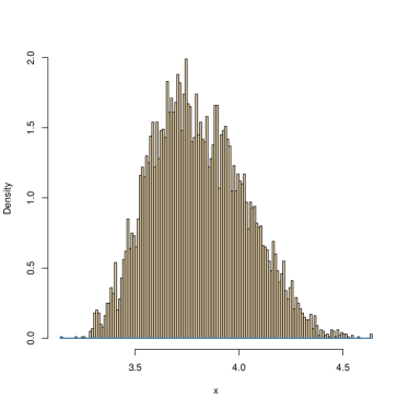
Figure 2: Fit of the histogram of a Metropolis–Hastings sample to its target, for $T=10^{4}$ iterations, a scale $\alpha=0.1$, and a starting value $x^{(1)}=3.14$.

Before describing the algorithm itself, let us stress the probabilistic foundations of Markov chain Monte Carlo (MCMC) algorithms: the Markov chain returned by the method, $X^{(1)},X^{(2)},\ldots,X^{(t)},\ldots$ is such that $X^{(t)}$ is converging to $\pi$. This means that the chain can be considered as a sample, albeit a dependent sample, and approximately distributed from $\pi$. Due to the Markovian nature of the simulation, the first values are highly dependent on the starting value $X^{(1)}$ and usually removed from the sample as burn-in or warm-up. While there are very few settings where the time when the chain reaches stationarity can be determined, see, e.g., Hobert and Robert (2004), there is no need to look for such an instant since the empirical average

$$\hat{\mathfrak{I}}_{T}(h)=\dfrac{1}{T}\sum_{t=1}^{T}h(X^{(t)})$$ (1)

converges almost surely to $\mathfrak{I}(h)$, no matter what the starting value, if the Markov chain is ergodic, i.e., forgets about its starting value. This implies that, in theory, simulating a Markov chain is intrinsically equivalent to a standard i.i.d. simulation from the target, the difference being in a loss of efficiency, i.e., in the necessity to simulate more terms to achieve a given variance for the above Monte Carlo estimator. The foundational principle for MCMC algorithms is thus straightforward, even though the practical implementation of the method may prove delicate or in cases impossible.

Without proceeding much further into Markov chain theory, we stress that the existence of a stationary distribution for a chain implies this chain automatically enjoys a strong stability called irreducibility. Namely, the chain can move all over the state space, i.e., can eventually reach any region of the state space, no matter its initial value.

2.2 The algorithm

The Metropolis–Hastings algorithm associated with a target density $\pi$ requires the choice of a conditional density $q$ also called proposal or candidate kernel. The transition from the value of the Markov chain $(X^{(t)})$ at time $t$ and its value at time $t+1$ proceeds via the following transition step:

Algorithm 1.

Metropolis–Hastings
Given $X^{(t)}=x^{(t)}$,

1. Generate $\;Y_{t}\sim q(y|x^{(t)})$.

2. Take

   $$X^{(t+1)}=\begin{cases}Y_{t}&\hbox{{\tt with probability} }\ \rho(x^{(t)},Y_{t}),\cr x^{(t)}&\hbox{{\tt with probability} }\ 1-\rho(x^{(t)},Y_{t}),\cr\end{cases}$$

   where

   $$\rho(x,y)=\min\left\{\dfrac{\tilde{\pi}(y)}{\tilde{\pi}(x)}\;\dfrac{q(x|y)}{q(y|x)}\;,1\right\}\,.$$

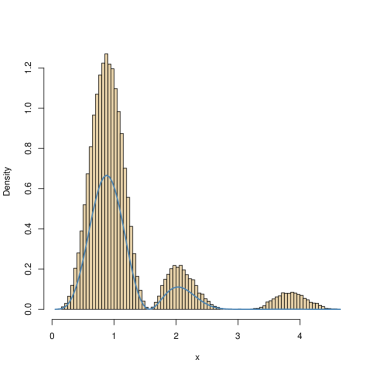
Figure 3: Fit of the histogram of a Metropolis–Hastings sample to its target, for $T=10^{5}$ iterations, a scale $\alpha=0.2$, and a starting value $x^{(1)}=3.14$.

Then, as shown in Metropolis et al. (1953), this transition preserves the stationary density $\pi$ if the chain is irreducible, that is, if $q$ has a wide enough support to eventually reach any region of the state space $\mathcal{X}$ with positive mass under $\pi$. A sufficient condition is that $q$ is positive everywhere. The very nature of accept-reject step introduced by those authors is therefore sufficient to turn a simulation from an almost arbitrary proposal density $q$ into a generation that preserves $\pi$ as the stationary distribution. This sounds both amazing and too good to be true! But it is true, in the theoretical sense drafted above. In practice, the performances of the algorithm are obviously highly dependent on the choice of the transition $q$, since some choices see the chain unable to converge in a manageable time.

2.3 An experiment with the algorithm

To capture the mechanism behind the algorithm, let us consider an elementary example:

Example 1.

Our target density is a perturbed version of the normal $\mathcal{N}(0,1)$ density, $\varphi(\cdot)$,

$$\tilde{\pi}(x)=\sin^{2}(x)\times\sin^{2}(2x)\times\varphi(x)\,.$$

And our proposal is a uniform $\mathcal{U}(x-\alpha,x+\alpha)$ kernel,

$$q(y|x)=\frac{1}{2\alpha}\mathbb{I}_{(x-\alpha,x+\alpha)}(y)\,.$$

Implementing this algorithm is straightforward: two functions to define are the target and the transition

target=function(x){
  sin(x)^2*sin(2*x)^2*dnorm(x)}

metropolis=function(x,alpha=1){
  y=runif(1,x-alpha,x+alpha)
  if (runif(1)>target(y)/target(x)) y=x
  return(y)}

and all we need is a starting value

T=10^4
x=rep(3.14,T)
for (t in 2:T) x[t]=metropolis(x[t-1])

which results in the histogram of Figure 1, where the target density is properly normalised by a numerical integration. If we look at the sequence $(x^{(t)})$ returned by the algorithm, it changes values around $5000$ times. This means that one proposal out of two is rejected. If we now change the scale of the uniform to $\alpha=0.1$, the chain $(x^{(t)})$ takes more than $9000$ different values, however the histogram in Figure 2 shows a poor fit to the target in that only one mode is properly explored. The proposal lacks the power to move the chain far enough to reach the other parts of the support of $\pi(\cdot)$. A similar behaviour occurs when we start at $0$. A last illustration of the possible drawbacks of using this algorithm is shown on Figure 3: when using the scale $\alpha=0.2$ the chain is slow in exploring the support, hence does not reproduce the correct shape of $\pi$ after $T=10^{5}$ iterations. $\blacktriangleleft$

From this example, we learned that some choices of proposal kernels work well to recover the shape of the target density, while others are poorer, and may even fail altogether to converge. Details about the implementation of the algorithm and the calibration of the proposal $q$ are detailed in Section 3.

2.4 Historical interlude

The initial geographical localisation of the MCMC algorithms is the nuclear research laboratory in Los Alamos, New Mexico, which work on the hydrogen bomb eventually led to the derivation Metropolis algorithm in the early 1950s. What can be reasonably seen as the first MCMC algorithm is indeed the Metropolis algorithm, published by Metropolis et al. (1953). Those algorithms are thus contemporary with the standard Monte Carlo method, developped by Ulam and von Neumann in the late 1940s. (Nicolas Metropolis is also credited with suggesting the name “Monte Carlo“, see Eckhardt, 1987, and published the very first Monte Carlo paper, see Metropolis and Ulam, 1949.) This Metropolis algorithm, while used in physics, was only generalized by Hastings (1970) and Peskun (1973, 1981) towards statistical applications, as a method apt to overcome the curse of dimensionality penalising regular Monte Carlo methods. Even those later generalisations and the work of Hammersley, Clifford, and Besag in the 1970’s did not truly impact the statistical community until Geman and Geman (1984) experimented with the Gibbs sampler for image processing, Tanner and Wong (1987) created a form of Gibbs sampler for latent variable models and Gelfand and Smith (1990) extracted the quintessential aspects of Gibbs sampler to turn it into a universal principle and rekindle the appeal of the Metropolis–Hastings algorithm for Bayesian computation and beyond.

3 Implementation details

When working with a Metropolis–Hastings algorithm, the generic nature of Algorithm 1 is as much an hindrance as a blessing in that the principle remains valid for almost every choice of the proposal $q$. It thus does not give indications about the calibration of this proposal. For instance, in Example 1, the method is valid for all choices of $\alpha$ but the comparison of the histogram of the outcome with the true density shows that $\alpha$ has a practical impact on the convergence of the algorithm and hence on the number of iterations it requires. Figure 4 illustrates this divergence in performances via the autocorrelation graphs of three chains produced by the R code in Example 1 for three highly different values of $\alpha=0.3,3,30$. It shows why $\alpha=3$ should be prefered to the other two values in that each value of the Markov chain contains “more” information in that case. The fundamental difficulty when using the Metropolis–Hastings algorithm is in uncovering which calibration is appropriate without engaging into much experimentation or, in other words, in an as automated manner as possible.

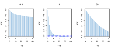
Figure 4: Comparison of the acf of three Markov chains corresponding to scales $\alpha=0.3,3,30$, for $T=10^{4}$ iterations, and a starting value $x^{(1)}=3.14$.

A (the?) generic version of the Metropolis–Hastings algorithm is the random walk Metropolis–Hastings algorithm, which exploits as little as possible knowledge about the target distribution, proceeding instead in a local if often myopic manner. To achieve this, the proposal distribution $q$ aims at a local exploration of the neighborhood of the current value of the Markov chain, i.e., simulating the proposed value $Y_{t}$ as

$$Y_{t}=X^{(t)}+\varepsilon_{t},$$

where $\varepsilon_{t}$ is a random perturbation with distribution $g$, for instance a uniform distribution as in Example 1 or a normal distribution. If we call random walk Metropolis–Hastings algorithms all the cases when $g$ is symmetric, the acceptance probability in Algorithm 1 gets simplified into

$$\rho(x,y)=\min\left\{\dfrac{\tilde{\pi}(y)}{\tilde{\pi}(x)}\;,1\right\}\,.$$

While this probability is independent of the scale of the proposal $g$, we just saw that the performances of the algorithm are quite dependent on such quantities. In order to achieve an higher degree of efficiency, i.e., towards a decrease of the Monte Carlo variance, Roberts et al. (1997) studied a formal Gaussian setting aiming at the ideal acceptance rate. Indeed, Example 1 showed that acceptance rates that are either “too high” or “too low” slow down the convergence of the Markov chain. They then showed that the ideal variance in the proposal is twice the variance of the target or, equivalently, that the acceptance rate should be close to $\nicefrac{{1}}{{4}}$. While this rule is only an indication (in the sense that it was primarily designed for a specific and asymptotic Gaussian environment), it provides a golden rule for the default calibration of random walk Metropolis–Hastings algorithms.

3.1 Effective sample size

We now consider the alternative of the effective sample size for comparing and calibrating MCMC algorithms. Even for a stationary Markov chain, using $T$ iterations does not amount to simulating an iid sample from $\pi$ that would lead to the same variability. Indeed, the empirical average (1) cannot be associated with the standard variance estimator

$$\hat{\sigma}^{2}_{T}=\frac{1}{T-1}\sum_{t=1}^{T}\left(h(X^{(t)})-\hat{\mathfrak{I}}_{T}(h)_{T}\right)^{2}$$

due to the correlations amongst the $X^{(t)}$’s. In this setting, the effective sample size is defined as the correction factor $\tau_{T}$ such that $\hat{\sigma}^{2}_{T}/\tau_{T}$ is the variance of the empirical average (1)). This quantity can be computed as in Geweke (1992) and Heidelberger and Welch (1983) by

$$\tau_{T}=T/\kappa(h)\,,$$

where $\kappa(h)$ is the autocorrelation associated with the sequence $h(X^{(t)})$,

$$\kappa(h)=1+2\,\sum_{t=1}^{\infty}\hbox{corr}\left(h(X^{(0)}),h(X^{(t)})\right)\,,$$

estimated by spectrum0 and effectiveSize from the R library coda, via the spectral density at zero. A rough alternative is to rely on subsampling, as in Robert and Casella (2009), so that $X^{(t+G)}$ is approximately independent from $X^{(t)}$. The lag $G$ is possibly determined in R via the autocorrelation function autocorr.

Example 2.

(Example 1 continued) We can compare the Markov chains obtained with $\alpha=0.3,3,30$ against those two criteria:

> autocor(mcmc(x))
            [,1] Ψ[,2]Ψ[,3]
Lag 0  1.0000000 1.0000000 1.0000000
Lag 1  0.9672805 0.9661440 0.9661440
Lag 5  0.8809364 0.2383277 0.8396924
Lag 10 0.8292220 0.0707092 0.7010028
Lag 50 0.7037832 -0.033926 0.1223127
> effectiveSize(x)
      [,1]       [,2]       [,3]
  33.45704 1465.66551  172.17784

This shows how much comparative improvement is brought by the value $\alpha=3$, but also that even this quasi-optimal case is far from an i.i.d. setting. $\blacktriangleleft$

3.2 In practice

In practice, the above tools of ideal acceptance rate and of higher effective sample size give goals for calibrating Metropolis–Hastings algorithms. This means comparing a range of values of the parameters involved in the proposal and selecting the value that achieves the highest target for the adopted goal. For a multidimensional parameter, global maximisation run afoul of the curse of dimensionality as exploring a grid of possible values quickly becomes impossible. The solution to this difficulty stands in running partial optimisations, with simulated (hence controlled) data, for instance setting all parameters but one fixed to the values used for the simulated data. If this is not possible, optimisation of the proposal parameters can be embedded in a Metropolis-within-Gibbs since for each step several values of the corresponding parameter can be compared via the Metropolis–Hastings acceptance probability.

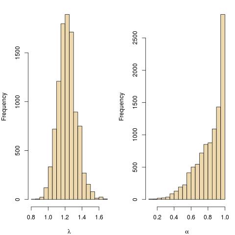
Figure 5: Output of a two-dimensional random walk Metropolis–Hastings algorithm for 123 observations from a Poisson distribution with mean $1$, under the assumed model of a mixture between Poisson and Geometric distributions.

We refer the reader to Chapter 8 of Robert and Casella (2009) for more detailed descriptions of the calibration of MCMC algorithms, including the use of adaptive mecchanisms. Indeed, calibration is normaly operated in a warm-up stage since, otherwise, if one continuously tune an MCMC algorithm according to its past outcome, the algorithm stops being Markovian. In order to preserve convergence in an adaptive MCMC algorithm, the solution found in the literature for this difficulty is to progressively tone/tune down the adaptive aspect. For instance, Roberts and Rosenthal (2009) propose a diminishing adaptation condition that states that the distance between two consecutive Markov kernels must uniformly decrease to zero. For instance, a random walk proposal that relies on the empirical variance of the past sample as suggested in Haario et al. (1999) does satisfy this condition. An alternative proposed by Roberts and Rosenthal (2009) proceeds by tuning the scale of a random walk for each component against the acceptance rate, which is the solution implemented in the amcmc package developed by Rosenthal (2007).

4 Illustration

Kamary et al. (2014) consider the special case of a mixture of a Poisson and of a Geometric distributions with the same mean parameter $\lambda$:

$$\alpha\mathcal{P}(\lambda)+(1-\alpha)\mathcal{G}eo(\nicefrac{{1}}{{1+\lambda}})\,,$$

where $\lambda>0$ and $0\leq\alpha\leq 1$. Given $n$ observations $(x_{1},\ldots,x_{n})$ and a prior decomposed into $\pi(\lambda)\propto\nicefrac{{1}}{{\lambda}}$ and $\pi(\alpha)\propto[\alpha(1-\alpha)]^{a_{0}-1}$, $a_{0}=0.5$ being the default value, the likelihood function is available in closed form as

$$\prod_{i=1}^{n}\left\{\alpha\frac{\lambda^{x_{i}}}{x_{i}!}\exp\{-\lambda\}+(1-\alpha)\lambda^{x_{i}}(1+\lambda)^{-x_{i}-1}\right\}$$

where $s_{n}=x_{1}+\ldots+x_{n}$. In R code, this translates as

likelihood=function(x,lam,alp){
  prod(alp*dpois(x,lam)+(1-alp)*dgeom(x,lam/(1+lam)))}
posterior=function(x,lam,alp){
  sum(log(alp*dpois(x,lam)+(1-alp)*dgeom(x,1/(1+lam))))-
      log(lam)+dbeta(alp,.5,.5,log=TRUE)}

If we want to build a Metropolis–Hastings algorithm that simulates from the associated posterior, the proposal can proceed by either proposing a joint move on $(\alpha,\lambda)$ or moving one parameter at a time in a Metropolis-within-Gibbs fashion. In the first case, we can imagine a random walk in two dimensions,

$$\alpha^{\prime}\sim\mathcal{E}(\epsilon\alpha,\epsilon(1-\alpha))\,,\quad\lambda^{\prime}\sim\mathcal{LN}(\log(\lambda),\delta(1+\log(\lambda)^{2}))\,,\qquad\epsilon\,,\delta>0$$

with an acceptance probability

$$\dfrac{\pi(\alpha^{\prime},\lambda^{\prime}|x)q(\alpha,\lambda|\alpha^{\prime},\lambda^{\prime})}{\pi(\alpha,\lambda|x)q(\alpha,\lambda|\alpha^{\prime},\lambda^{\prime})}\wedge 1\,.$$

The Metropolis–Hastings R code would then be

metropolis=function(x,lam,alp,eps=1,del=1){
  prop=c(exp(rnorm(1,log(lam),sqrt(del*(1+log(lam)^2)))),
         rbeta(1,1+eps*alp,1+eps*(1-alp)))
  rat=posterior(x,prop[1],prop[2])-posterior(x,lam,alp)+
         dbeta(alp,1+eps*prop[2],1+eps*(1-prop[2]),log=TRUE)-
         dbeta(prop[2],1+eps*alp,1+eps*(1-alp),log=TRUE)+
         dnorm(log(lam),log(prop[1]),
               sqrt(del*(1+log(prop[1])^2)),log=TRUE)-
         dnorm(log(prop[1]),log(lam),
               sqrt(del*(1+log(lam)^2)),log=TRUE)+
         log(prop[1]/lam)
  if (log(runif(1))>rat) prop=c(lam,alp)
  return(prop)}

where the ratio prop[1]/lam in the acceptance probability is just the Jacobian for the log-normal transform. Running the following R code

T=1e4
x=rpois(123,lambda=1)
para=matrix(c(mean(x),runif(1)),nrow=2,ncol=T)
like=rep(0,T)
for (t in 2:T){
   para[,t]=metropolis(x,para[1,t-1],para[2,t-1],eps=.1,del=.1)
   like[t]=posterior(x,para[1,t],para[2,t])}

then produced the histograms of Figure 5, after toying with the values of $\epsilon$ and $\delta$ to achieve a large enough average acceptance probability, which is provided by length(unique(para[1,]))/T The second version of the Metropolis–Hastings algorithm we can test is to separately modify $\lambda$ by a random walk proposal, test whether or not it is acceptable, and repeat with $\alpha$: the R code is then very similar to the above one:

metropolis=function(x,lam,alp,eps=1,del=1){
  prop=exp(rnorm(1,log(lam),sqrt(del*(1+log(lam)^2))))
  rat=posterior(x,prop,alp)-posterior(x,lam,alp)+
         dnorm(log(lam),log(prop[1]),
               sqrt(del*(1+log(prop[1])^2)),log=TRUE)-
         dnorm(log(prop[1]),log(lam),
               sqrt(del*(1+log(lam)^2)),log=TRUE)+
         log(prop/lam)
  if (log(runif(1))>rat) prop=lam
  qrop=rbeta(1,1+eps*alp,1+eps*(1-alp))
  rat=posterior(x,prop,qrop)-posterior(x,prop,alp)+
         dbeta(alp,1+eps*qrop,1+eps*(1-qrop),log=TRUE)-
         dbeta(qrop,1+eps*alp,1+eps*(1-alp),log=TRUE)
  if (log(runif(1))>rat) qrop=alp
  return(c(prop,qrop))}

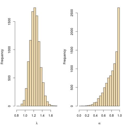
Figure 6: Output of a Metropolis-within-Gibbs random walk Metropolis–Hastings algorithm for 123 observations from a Poisson distribution with mean $1$, under the assumed model of a mixture between Poisson and Geometric distributions.

In this special case, both algorithms thus return mostly equivalent outcomes, with a slightly more dispersed output in the case of the Metropolis-within-Gibbs version (Figure 7). In a more general perspective, calibrating random walks in multiple dimensions may prove unwieldly, especially with large dimensions, while the Metropolis-within-Gibbs remains manageable. One drawback of the later is common to all Gibbs implementations, namely that it induces higher correlations between the components, which means a slow convergence of the chain (and in extreme cases no convergence at all).

5 Extensions

5.1 Langevin algorithms

An extension of the random walk Metropolis–Hastings algorithm is based on the Langevin diffusion solving

$$\text{d}X_{t}=\nicefrac{{1}}{{2}}\nabla\log\pi(X_{t})\text{d}t+\text{d}B_{t}\,,$$

where $B_{t}$ is the standard Brownian motion and $\nabla f$ denotes the gradient of $f$, since this diffusion has $\pi$ as its stationary and limiting distribution. The algorithm is based on a discretised version of the above, namely

$$Y_{n+1}|X_{n}\sim\mathcal{N}\left(x+\nicefrac{{h}}{{2}}\nabla\log\pi(x),h^{\nicefrac{{1}}{{2}}}\,I_{d}\right)\,,$$

for a discretisation step $h$, which is used as a proposed value for $X_{n+1}$, and accepted with the standard Metropolis–Hastings probability (Roberts and Tweedie, 1995). This new proposal took the name of Metropolis adjusted Langevin algorithms (hence MALA). While computing (twice) the gradient of $\pi$ at each iteration requires extra time, there is strong support for doing so, as MALA algorithms do provide noticeable speed-ups in convergence for most problems. Note that $\pi(\cdot)$ only needs to be known up to a multiplicative constant because of the log transform.

5.2 Particle MCMC

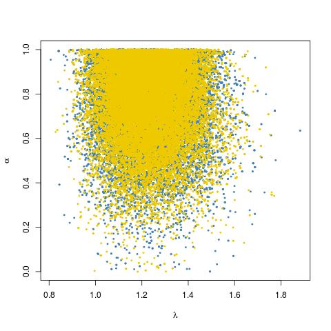
Figure 7: Output of a Metropolis-within-Gibbs (blue) and of a two-dimensional (gold) random walk Metropolis–Hastings algorithm for 123 observations from a Poisson distribution with mean $1$, under the assumed model of a mixture between Poisson and Geometric distributions.

Another extension of the Metropolis–Hastings algorithm is the particle MCMC (or pMCMC), developed by Andrieu et al. (2011). While we cannot provide an introduction to particle filters here, see, e.g., Del Moral et al. (2006), we want to point out the appeal of this approach in state space models like hidden Markov models (HMM). This innovation is similar to the pseudo-marginal algorithm approach of Beaumont (2003); Andrieu and Roberts (2009), taking advantage of the auxiliary variables exploited by particle filters.

In the case of an HMM, i.e., where a latent Markov chain $x_{0:T}$ with density

$$p_{0}(x_{0}|\theta)p_{1}(x_{1}|x_{0},\theta)\cdots p_{T}(x_{T}|x_{T-1},\theta)\,,$$

is associated with an observed sequence $y_{1+T}$ such that

$$y_{1+T}|X_{1:T},\theta\sim\prod_{i=1}^{T}q_{i}(y_{i}|x_{i},\theta)\,,$$

pMCMC applies as follows. At every iteration $t$, a value $\theta^{\prime}$ of the parameter $\theta\sim\mathfrak{h}(\theta|\theta^{(t)})$ is proposed, followed by a new value of the latent series $x_{0:T}^{\prime}$ generated from a particle filter approximation of $p(x_{0:T}|\theta^{\prime},y_{1:T})$. As the particle filter produces in addition (Del Moral et al., 2006) an unbiased estimator of the marginal posterior of $y_{1:T}$, $\hat{q}(y_{1:T}|\theta^{\prime})$, this estimator can be directly included in the Metropolis–Hastings ratio

$$\dfrac{\hat{q}(y_{1:T}|\theta^{\prime})\pi(\theta^{\prime})\mathfrak{h}(\theta^{(t)}|\theta^{\prime})}{\hat{q}(y_{1:T}|\theta)\pi(\theta^{(t)})\mathfrak{h}(\theta^{\prime}|\theta^{(t)})}\wedge 1\,.$$

The validation of this substitution follows from the general argument of Andrieu and Roberts (2009) for pseudo-marginal techniques, even though additional arguments are required to establish that all random variables used therein are accounted for (see Andrieu et al., 2011 and Wilkinson, 2011). We however stress that the general validation of those algorithm as converging to the joint posterior does not proceed from pseudo-marginal arguments. An extension of pMCMC called $\text{SMC}^{2}$ that approximates the sequential filtering distribution is proposed in Chopin et al. (2013).

5.3 Pseudo-marginals

As illustrated by the previous section, there are many settings where computing the target density $\pi(\cdot)$ is impossible. Another example is made of doubly intractable likelihoods (Murray et al., 2006a), when the likelihood function contains a term that is intractable, for instance $\ell(\theta|x)\propto g(x|\theta)$ with an intractable normalising constant

$$\mathfrak{Z}(\theta)=\int_{\mathcal{X}}g(x|\theta)\,\text{d}x\,.$$

This phenomenon is quite common in graphical models, as for instance for the Ising model (Murray et al., 2006b; Møller et al., 2006). Solutions based on auxiliary variables have been proposed (see, e.g., Murray et al., 2006a; Møller et al., 2006), but they may prove difficult to calibrate.

In such settings, Andrieu and Roberts (2009) developped an approach based on an idea of Beaumont (2003), designing a valid Metropolis–Hastings algorithm that substitutes the intractable target $\pi(\cdot|x)$ with an unbiased estimator. A slight change to the Metropolis–Hastings acceptance ratio ensures that the stationary density of the corresponding Markov chain is still equal to the target $\pi$. Indeed, provided $\hat{\pi}(\theta|z)$ is an unbiased estimator of $\pi(\theta)$ when $z\sim q(\cdot|\theta)$, it is rather straightforward to check that the acceptance ratio

$$\dfrac{\hat{\pi}(\theta^{*}|z^{*})}{\hat{\pi}(\theta|z)}\,\dfrac{q(\theta^{*},\theta)q(z|\theta)}{q(\theta,\theta^{*})q(z^{*}|\theta^{*})}$$

preserves stationarity with respect to an extended target (see Andrieu and Roberts (2009)) for details) when $z^{*}\sim q(\cdot|\theta)$, and $\theta^{*}|\theta\sim q(\theta,\theta^{*})$. Andrieu and Vihola (2015) propose an alternative validation via auxiliary weights used in the unbiased estimation, assuming the unbiased estimator (or the weight) is generated conditional on the proposed value in the original Markov chain. The performances of pseudo-marginal solutions depend on the quality of the estimators $\hat{\pi}$ and are always poorer than when using the exact target $\pi$. In particular, improvements can be found by using multiple samples of $z$ to estimate $\pi$ (Andrieu and Vihola, 2015).

6 Conclusion and new directions

The Metropolis–Hastings algorithm is to be understood as a default or off-the-shelf solution, meaning that (a) it rarely achieves optimal rates of convergence (Mengersen and Tweedie, 1996) and may get into convergence difficulties if improperly calibrated but (b) it can be combined with other solutions as a baseline solution, offering further local or more rarely global exploration to a taylored algorithm. Provided reversibility is preserved, it is indeed valid to mix several MCMC algorithms together, for instance picking one of the kernels at random or following a cycle (Tierney, 1994; Robert and Casella, 2004). Unless a proposal is relatively expensive to compute or to implement, it rarely hurts to add an extra kernel into the MCMC machinery.

This is not to state that the Metropolis–Hastings algorithm is the ultimate solution to all simulation and stochastic evaluation problems. For one thing, there exist settings where the intractability of the target is such that no practical MCMC solution is available. For another thing, there exist non reversible versions of those algorithms, like Hamiltonian (or hybrid) Monte Carlo (HMC) (Duane et al., 1987; Neal, 2013; Betancourt et al., 2014). This method starts by creating a completly artificial variable $p$, inspired by the momentum in physics, and a joint distribution on $(q,p)$ which energy—minus the log-density—is defined by the Hamiltonian

$$H(q,p)=-\log\pi(q)+p^{\text{T}}M^{-1}p/2\,,$$

where $M$ is the so-called mass matrix. The second part in the target is called the kinetic energy, still by analogy with mechanics. When the joint vector $(q,p)$ is driven by Hamilton’s equations

$$\dfrac{\text{d}q}{\text{d}t} =\dfrac{\partial H}{\partial p}=\dfrac{\partial H}{\partial p}=M^{-1}p$$

$$\dfrac{\text{d}p}{\text{d}t} =-\dfrac{\partial H}{\partial q}=\dfrac{\partial\log\pi}{\partial q}$$

this dynamics preserves the joint distribution with density $\exp-H(p,q)$. If we could simulate exactly from this joint distribution of $(q,p)$, a sample from $\pi(q)$ would be a by-product. In practice, the equation is only solved approximately and hence requires a Metropolis–Hastings correction. Its practical implementation is called the leapfrog approximation (Neal, 2013; Girolami and Calderhead, 2011) as it relies on a small discretisation step $\epsilon$, updating $p$ and $q$ via a modified Euler’s method called the leapfrog that is reversible and preserves volume as well. This discretised update can be repeated for an arbitrary number of steps.

The appeal of HMC against other MCMC solutions is that the value of the Hamiltonian changes very little during the Metropolis step, while possibly producing a very different value of $q$. Intuitively, moving along level sets in the augmented space is almost energy-free, but if those move proceeds far enough, the Markov chain on $q$ can reach distant regions, thus avoid the typical local nature of regular MCMC algorithms. This strengthe explains in part why a statistical software like STAN (Stan Development Team, 2014) is mostly based on HMC moves.

As a last direction for new MCMC solutions, let us point out the requirements set by Big Data, i.e., in settings where the likelihood function cannot be cheaply evaluated for the entire dataset. See, e.g., Scott et al. (2013); Wang and Dunson (2013), for recent entries on different parallel ways of handling massive datasets, and Brockwell (2006); Strid (2010); Banterle et al. (2015) for delayed and prefetching MCMC techniques that avoid considering the entire likelihood at once.

References

- Andrieu et al. (2011) Andrieu, C., Doucet, A., and Holenstein, R. (2011). “Particle Markov chain Monte Carlo (with discussion).” J. Royal Statist. Society Series B, 72 (2): 269–342.
- Andrieu and Roberts (2009) Andrieu, C. and Roberts, G. (2009). “The pseudo-marginal approach for efficient Monte Carlo computations.” Ann. Statist., 37(2): 697–725.
- Andrieu and Vihola (2015) Andrieu, C. and Vihola, M. (2015). “Convergence properties of pseudo-marginal Markov chain Monte Carlo algorithms.” Ann. Applied Probab., 25(2): 1030–1077.
- Banterle et al. (2015) Banterle, M., Grazian, C., Lee, A., and Robert, C. P. (2015). “Accelerating Metropolis-Hastings algorithms by Delayed Acceptance.” ArXiv e-prints.
- Barker (1965) Barker, A. (1965). “Monte Carlo calculations of the radial distribution functions for a proton electron plasma.” Aust. J. Physics, 18: 119–133.
- Beaumont (2003) Beaumont, M. (2003). “Estimation of population growth or decline in genetically monitored populations.” Genetics, 164: 1139–1160.
- Betancourt et al. (2014) Betancourt, M. J., Byrne, S., Livingstone, S., and Girolami, M. (2014). “The Geometric Foundations of Hamiltonian Monte Carlo.” ArXiv e-prints.
- Brockwell (2006) Brockwell, A. (2006). “Parallel Markov chain Monte Carlo Simulation by Pre-Fetching.” J. Comput. Graphical Stat., 15(1): 246–261.
- Chopin et al. (2013) Chopin, N., Jacob, P. E., and Papaspiliopoulos, O. (2013). “SMC2: an efficient algorithm for sequential analysis of state space models.” J. Royal Statist. Society Series B, 75(3): 397–426.
- Del Moral et al. (2006) Del Moral, P., Doucet, A., and Jasra, A. (2006). “Sequential Monte Carlo samplers.” J. Royal Statist. Society Series B, 68(3): 411–436.
- Duane et al. (1987) Duane, S., Kennedy, A. D., Pendleton, B. J., , and Roweth, D. (1987). “Hybrid Monte Carlo.” Phys. Lett. B, 195: 216–222.
- Eckhardt (1987) Eckhardt, R. (1987). “Stan Ulam, John Von Neumann, and the Monte Carlo Method.” Los Alamos Science, Special Issue, 131–141.
- Gelfand and Smith (1990) Gelfand, A. and Smith, A. (1990). “Sampling based approaches to calculating marginal densities.” J. American Statist. Assoc., 85: 398–409.
- Geman and Geman (1984) Geman, S. and Geman, D. (1984). “Stochastic relaxation, Gibbs distributions and the Bayesian restoration of images.” IEEE Trans. Pattern Anal. Mach. Intell., 6: 721–741.
- Geweke (1992) Geweke, J. (1992). “Evaluating the accuracy of sampling-based approaches to the calculation of posterior moments (with discussion).” In Bernardo, J., Berger, J., Dawid, A., and Smith, A. (eds.), Bayesian Statistics 4, 169–193. Oxford: Oxford University Press.
- Girolami and Calderhead (2011) Girolami, M. and Calderhead, B. (2011). “Riemann manifold Langevin and Hamiltonian Monte Carlo methods.” Journal of the Royal Statistical Society: Series B (Statistical Methodology), 73: 123–214.
- Haario et al. (1999) Haario, H., Saksman, E., and Tamminen, J. (1999). “Adaptive Proposal Distribution for Random Walk Metropolis Algorithm.” Computational Statistics, 14(3): 375–395.
- Hammersley and Handscomb (1964) Hammersley, J. and Handscomb, D. (1964). Monte Carlo Methods. New York: John Wiley.
- Hastings (1970) Hastings, W. (1970). “Monte Carlo sampling methods using Markov chains and their application.” Biometrika, 57: 97–109.
- Heidelberger and Welch (1983) Heidelberger, P. and Welch, P. (1983). “A spectral method for confidence interval generation and run length control in simulations.” Comm. Assoc. Comput. Machinery, 24: 233–245.
- Hobert and Robert (2004) Hobert, J. and Robert, C. (2004). “A mixture representation of with applications in Markov chain Monte Carlo and perfect sampling.” Ann. Applied Prob., 14: 1295–1305.
- Kamary et al. (2014) Kamary, K., Mengersen, K., Robert, C., and Rousseau, J. (2014). “Testing hypotheses as a mixture estimation model.” arxiv:1214.2044.
- Mengersen and Tweedie (1996) Mengersen, K. and Tweedie, R. (1996). “Rates of convergence of the Hastings and Metropolis algorithms.” Ann. Statist., 24: 101–121.
- Metropolis et al. (1953) Metropolis, N., Rosenbluth, A., Rosenbluth, M., Teller, A., and Teller, E. (1953). “Equations of state calculations by fast computing machines.” J. Chem. Phys., 21(6): 1087–1092.
- Metropolis and Ulam (1949) Metropolis, N. and Ulam, S. (1949). “The Monte Carlo method.” J. American Statist. Assoc., 44: 335–341.
- Meyn and Tweedie (1994) Meyn, S. and Tweedie, R. (1994). “Computable bounds for convergence rates of Markov chains.” Ann. Appl. Probab., 4: 981–1011.
- Møller et al. (2006) Møller, J., Pettitt, A. N., Reeves, R., and Berthelsen, K. K. (2006). “An efficient Markov chain Monte Carlo method for distributions with intractable normalising constants.” Biometrika, 93(2): 451–458.
- Murray et al. (2006a) Murray, I., Ghahramani, Z., , and MacKay, D. (2006a). “MCMC for doubly-intractable distributions.” In Uncertainty in Artificial Intelligence. UAI-2006.
- Murray et al. (2006b) Murray, I., MacKay, D. J., Ghahramani, Z., and Skilling, J. (2006b). “Nested sampling for Potts models.” In Weiss, Y., Schölkopf, B., and Platt, J. (eds.), Advances in Neural Information Processing Systems 18, 947–954. Cambridge, MA: MIT Press.
- Neal (2013) Neal, R. (2013). “MCMC using Hamiltonian dynamics.” In Brooks, S., Gelman, A., Jones, G., and Meng, X.-L. (eds.), Handbook of Markov Chain Monte Carlo, 113–162. Chapman & Hall/CRC Press.
- Peskun (1973) Peskun, P. (1973). “Optimum Monte Carlo sampling using Markov chains.” Biometrika, 60: 607–612.
- Peskun (1981) — (1981). “Guidelines for chosing the transition matrix in Monte Carlo methods using Markov chains.” Journal of Computational Physics, 40: 327–344.
- Robert and Casella (2004) Robert, C. and Casella, G. (2004). Monte Carlo Statistical Methods. Springer-Verlag, New York, second edition.
- Robert and Casella (2009) — (2009). Introducing Monte Carlo Methods with R. Springer-Verlag, New York.
- Robert and Casella (2010) — (2010). “A history of Markov Chain Monte Carlo-Subjective recollections from incomplete data.” In Brooks, S., Gelman, A., Meng, X., and Jones, G. (eds.), Handbook of Markov Chain Monte Carlo, 49–66. Chapman and Hall, New York. ArXiv0808.2902.
- Roberts et al. (1997) Roberts, G., Gelman, A., and Gilks, W. (1997). “Weak convergence and optimal scaling of random walk Metropolis algorithms.” Ann. Applied Prob., 7: 110–120.
- Roberts and Rosenthal (2009) Roberts, G. and Rosenthal, J. (2009). “Examples of Adaptive MCMC.” J. Comp. Graph. Stat., 18: 349–367.
- Roberts and Tweedie (1995) Roberts, G. and Tweedie, R. (1995). “Exponential convergence for Langevin diffusions and their discrete approximations.” Technical report, Statistics Laboratory, Univ. of Cambridge.
- Rosenthal (2007) Rosenthal, J. (2007). “AMCM: An R interface for adaptive MCMC.” Comput. Statist. Data Analysis, 51: 5467–5470.
- Rubinstein (1981) Rubinstein, R. (1981). Simulation and the Monte Carlo Method. New York: John Wiley.
- Scott et al. (2013) Scott, S., Blocker, A., Bonassi, F., Chipman, H., George, E., and McCulloch, R. (2013). “Bayes and big data: The consensus Monte Carlo algorithm.” EFaBBayes 250 conference, 16.
- Stan Development Team (2014) Stan Development Team (2014). “STAN: A C++ Library for Probability and Sampling, Version 2.5.0, http://mc-stan.org/.”
- Strid (2010) Strid, I. (2010). “Efficient parallelisation of Metropolis–Hastings algorithms using a prefetching approach.” Computational Statistics & Data Analysis, 54(11): 2814–2835.
- Tanner and Wong (1987) Tanner, M. and Wong, W. (1987). “The calculation of posterior distributions by data augmentation.” J. American Statist. Assoc., 82: 528–550.
- Tierney (1994) Tierney, L. (1994). “Markov chains for exploring posterior distributions (with discussion).” Ann. Statist., 22: 1701–1786.
- Wang and Dunson (2013) Wang, X. and Dunson, D. (2013). “Parallizing MCMC via Weierstrass Sampler.” arXiv preprint arXiv:1312.4605.
- Wilkinson (2011) Wilkinson, D. (2011). “The particle marginal Metropolis–Hastings (PMMH) particle MCMC algorithm.” https://darrenjw.wordpress.com/2011/05/17/the-particle-marginal-metropolis-hastings-pmmh-particle-mcmc-algorithm/. Darren Wilkinson’s research blog.