Diffraction of waves by screens (apertures in screens) with time-varying dimensions. Time-varying Kirchhoff’s integral representation for moving boundaries

Abstract

The diffraction of electromagnetic waves by screens (apertures in screens) with time-varying dimensions is studied. The generalized vector Kirchhoff’s representation for this case is obtained. It is also shown that with accuracy up to the terms of the order of $\frac{v}{c}<<1$, the expressions for the scattered wave and instantaneous power can be derived from the appropriate expressions for a stationary case by substituting the time-dependent parameters of the screen dimensions (e.g. time-dependent radius) for constant parameters of screen dimensions (e.g., the screen radius) appearing in the formulas describing the stationary case.

1 Introduction

Diffraction of electromagnetic waves by different bodies and screens is the subject of multiple studies [1, 2]. The most important theoretical results on diffraction by metal screens and apertures were reported by Kirchhoff, Bethe, and Bouwkamp (see, for example, [1, 3, 4]). Recent research into electromagnetic wave transmission through an array of small holes [5] has renewed the interest in electromagnetic wave diffraction [5, 6, 7]. It should be mentioned that all the papers cited above considered the diffraction of electromagnetic waves by metal screens and apertures with time-constant dimensions.

In this paper we present – to my knowledge – the first theoretical study of diffraction of electromagnetic waves by screens (apertures in screens) with time-varying dimensions and obtain the generalized vector Kirchhoff representation for this case. Such diffraction case may occur, e.g., when the electromagnetic wave is incident on the aperture made in a metal screen by laser piercing, when the electromagnetic wave traverses the cylindrical metal shell collapsed under a Z-pinch, or when a metal wire irradiated with the electromagnetic wave is exploded under the action of a power current pulse running across it.

The paper is arranged as follows: Section 2 generalizes the scalar Kirchhoff’s integral representation to the case of screens and apertures with time-dependent dimensions. Section 3 discusses wave diffraction by the screen’s circular aperture with time-dependent radius. Section 4 studies diffraction by a sphere with time-dependent radius. Section 5 derives the time-dependent vector Kirchhoff’s representation describing the electromagnetic wave diffraction by a screen (aperture) with time-dependent dimensions.

2 Generalized scalar Kirchhoff’s integral representation for the case of screens and apertures with time-dependent dimensions

Let an electromagnetic wave be incident on a screen (aperture) with time-dependent dimensions. We shall first recall Green’s formula. According to Gauss’s flux theorem, for any vector field $\vec{A}(\vec{r})$ in the volume $V$ enclosed by the surface $S$ there holds the equality [10]

$$\int_{V}{\texttt{div}}\,\vec{A}(\vec{r})d^{3}r=\oint_{S}\vec{A}\vec{n}dS,$$ (1)

where $\vec{n}$ is the unit normal vector to the surface, which is directed outside the volume.

Following [1], we shall begin the consideration from the diffraction of a scalar field, with $\psi$ denoting one of the electromagnetic-field components. (It should be mentioned that for the case of scalar wave propagation, the extension of the Kirchhoff’s scalar formula to apply to moving surfaces in acoustics was obtained in [8, 9].) Let $\vec{A}=\varphi\vec{\nabla}\psi$, where $\varphi$ and $\psi$ are the arbitrary scalar functions. Then

$$\texttt{div}(\varphi\vec{\nabla}\psi)=\varphi\Delta\psi+\vec{\nabla}\varphi\cdot\vec{\nabla}\psi$$ (2)

and

$$\varphi(\vec{\nabla}\psi)\cdot\vec{n}=\varphi\frac{\partial\psi}{\partial n}=\varphi\vec{n}\vec{\nabla}\psi,$$ (3)

where $\frac{\partial}{\partial n}$ is the derivative on the surface $S$ taken along the direction of the outer normal relative to the volume $V$.

Let us substitute (2) and (3) into (1). After certain transformations (for details see, e.g., [1]), we obtain the equality called Green’s theorem [1]:

$$\int_{V}(\varphi\Delta\psi-\psi\Delta\varphi)d^{3}r=\oint_{S}\left[\varphi\frac{\partial\varphi}{\partial n}-\psi\frac{\partial\varphi}{\partial n}\right]dS.$$ (4)

Let us assume that the volume $V$ and the surface $S$ are time-independent. In this case, according to [1], we can recast the wave equation

$$\Delta\psi-\frac{1}{c^{2}}\frac{\partial^{2}\psi}{\partial t^{2}}=-4\pi f(\vec{r},t)$$ (5)

in the integral form ($c$ is the speed of light, $f(\vec{r},t)$ is the distribution density of the sources) that enables us to write the solution of the wave equation for $\psi(r,t)$ using explicitly the initial conditions $\psi(\vec{r},t_{0})$ and $\frac{\partial\psi(\vec{r},t)}{\partial t}|_{t>t_{0}}$, as well as the boundary conditions on the surface [1]. This integral form of wave equation is known as the scalar Kirchhoff’s integral representation.

Because in the case under consideration the volume $V$ and the surface $S$ are time-dependent, we need to choose a different method of obtaining the integral equation.

We shall integrate the left- and right-hand sides of (4) between the time limits $[t_{0},t_{1}]$ (compare with [1] ). In this case, we can obtain from (4)

$$\int_{t_{0}}^{t_{1}}dt^{\prime}\int_{V(t^{\prime})}d^{3}r^{\prime}(\varphi\Delta\psi-\psi\Delta\varphi)=\int_{t_{0}}^{t_{1}}dt^{\prime}\oint_{S(t^{\prime})}\left(\varphi\frac{\partial\psi}{\partial n^{\prime}}-\psi\frac{\partial\varphi}{\partial n^{\prime}}\right)dS.$$ (6)

We shall further assume that $\psi=\psi$ and $\varphi=G$, where $G$ is the Green function of the wave equation

$$\left(\Delta_{r}-\frac{1}{c^{2}}\frac{\partial^{2}}{\partial t^{2}}\right)G(\vec{r},t;\vec{r}\,^{\prime},t^{\prime})=-4\pi\delta(\vec{r}-\vec{r}\,^{\prime})\delta(t-t^{\prime}).$$ (7)

The upper limit of integration, $t_{1}$, is chosen to be greater than $t$: $t_{1}>t$. As a result, we can write:

$$\int_{t_{0}}^{t_{1}}dt^{\prime}\int_{V(t^{\prime})}d^{3}r^{\prime}\left[G(\vec{r},t;\vec{r}\,^{\prime},t^{\prime})\Delta_{r^{\prime}}\psi(\vec{r}\,^{\prime},t^{\prime})-\psi(\vec{r}\,^{\prime},t^{\prime})\Delta_{r^{\prime}}^{\prime}G(\vec{r},t;\vec{r}\,^{\prime},t^{\prime})\right]=$$

$$\int_{t_{0}}^{t_{1}}dt^{\prime}\int_{S(t^{\prime})}\left[G(\vec{r},t;\vec{r}\,^{\prime},t^{\prime})\frac{\partial\psi(\vec{r}\,^{\prime},t^{\prime})}{\partial n^{\prime}}-\psi(\vec{r}\,^{\prime},t^{\prime})\frac{\partial}{\partial n^{\prime}}G(\vec{r},t;\vec{r}\,^{\prime},t^{\prime})\right]dS^{\prime}.$$ (8)

Let us recall that in the right-hand side of equation (2) all points $\vec{r}\,^{\prime}$ lie on the the surface $S(t^{\prime})$ enclosing the volume $V(t^{\prime})$; $\frac{\partial\psi}{\partial n^{\prime}}=\vec{n}\,^{\prime}\frac{\partial\psi}{\partial\vec{r}\,^{\prime}}$. We shall make use of (5) and (7) and recast (2) as follows:

$$\int_{t_{0}}^{t_{1}}dt^{\prime}\int_{V(t^{\prime})}d^{3}r^{\prime}\left\{G(\vec{r},t;\vec{r}\,^{\prime},t^{\prime})\left[\frac{1}{c^{2}}\frac{\partial^{2}\psi(\vec{r}\,^{\prime},t^{\prime})}{\partial t^{\prime 2}}-4\pi f(\vec{r}\,^{\prime},t^{\prime})\right]\right.$$

$$-\left.\psi(\vec{r}\,^{\prime},t^{\prime})\left[\frac{1}{c^{2}}\frac{\partial^{2}}{\partial t^{\prime 2}}G(\vec{r},t;\vec{r}\,^{\prime},t^{\prime})-4\pi\delta(\vec{r}-\vec{r}\,^{\prime})\delta(t-t^{\prime})\right]\right\}$$ (9)

$$=\int_{t_{0}}^{t_{1}}dt^{\prime}\int_{S(t^{\prime})}\left[G(\vec{r},t;\vec{r}\,^{\prime},t^{\prime})\frac{\partial\psi(\vec{r}\,^{\prime},t^{\prime})}{\partial n^{\prime}}-\psi(\vec{r}\,^{\prime},t^{\prime})\frac{\partial}{\partial n^{\prime}}G(\vec{r},t;\vec{r}\,^{\prime},t^{\prime})\right]dS^{\prime},$$

that is,

$$4\pi\psi(\vec{r},t)-4\pi\int_{t_{0}}^{t_{1}}dt^{\prime}\int_{V(t^{\prime})}d^{3}r^{\prime}G(\vec{r},t;\vec{r}\,^{\prime},t^{\prime})f(\vec{r}\,^{\prime},t^{\prime})+$$

$$+ \int^{t_{1}}_{t_{0}}dt^{\prime}\int_{V(t^{\prime})}d^{3}r^{\prime}\left\{G(\vec{r},t;\vec{r}\,^{\prime},t^{\prime})\frac{1}{c^{2}}\frac{\partial^{2}\psi(\vec{r}\,^{\prime},t^{\prime})}{\partial t^{\prime 2}}-\psi(\vec{r}\,^{\prime},t^{\prime})\frac{1}{c^{2}}\frac{\partial^{2}}{\partial t^{\prime 2}}G(\vec{r},t;\vec{r}\,^{\prime},t^{\prime})\right\}=$$

$$= \int_{t_{0}}^{t_{1}}dt^{\prime}\int_{S(t^{\prime})}\left[G(\vec{r},t;\vec{r}\,^{\prime},t^{\prime})\frac{\partial\psi(\vec{r}\,^{\prime},t^{\prime})}{\partial n^{\prime}}-\psi(\vec{r}\,^{\prime},t^{\prime})\frac{\partial}{\partial n^{\prime}}G(\vec{r},t;\vec{r}\,^{\prime},t^{\prime})\right]dS^{\prime}$$

By changing the order of integration over $dt^{\prime}$ and $d^{3}r^{\prime}$, $dt^{\prime}$ and $dS^{\prime}$ we can obtain Kirchhoff’s integral representation (see [4, 5]), i.e., the integral equations for $\psi$, where the function $\psi$ is expressed in terms of the values of $\psi$ and its coordinate and time derivatives on the surface $S$. But this change of the order of integration is valid only in the case when the volume $V$ and the surface $S$ are time-independent! If $V=V(t)$ and $S=S(t)$, the order of integration cannot be changed. For this reason, we shall introduce the function $\Theta(\vec{r}\,^{\prime},\vec{R}(t^{\prime}))$ such that $\Theta(\vec{r}\,^{\prime},\vec{R}(t^{\prime}))=1$ for all points $\vec{r}^{\prime}$ contained in the volume $V(t^{\prime})$ enclosed by the surface $S(t^{\prime})$ that is described by the coordinates $\vec{R}(t^{\prime})$ of the points belonging to the surface; $\Theta(\vec{r}\,^{\prime},\vec{R}(t^{\prime}))=0$ for points $\vec{r}\,^{\prime}$ exterior to the volume $V(t^{\prime})$. Using this function, we can write the integral $\int_{{}_{V(t^{\prime})}}d^{3}r^{\prime}...$ over the time-dependent volume $V(t^{\prime})$ in the third term on the left-hand side of (2) in the form of the integral $\int d^{3}r^{\prime}\Theta(\vec{r}\,^{\prime},\vec{R}(t^{\prime}))...$, where integration is performed over a certain large (infinite in the limit) constant volume. As a result, we can perform time integration by parts on the left-hand side of (2) and transform the second-order derivatives into the first-order ones: $\frac{\partial^{2}}{\partial t^{\prime 2}}\longrightarrow\frac{\partial}{\partial t^{\prime}}$. This gives us the integral equation for the function $\psi(\vec{r},t)$ expressed in terms of the function $f(\vec{r},t)$, describing the radiation source, $\psi$ and the derivatives thereof on the surface enclosing the volume $V(t)$, as well as in terms of the initial value of $\psi(\vec{r},t_{0})$ and the derivative thereof at the initial time. The equation thus obtained generalizes Kirchhoff’s integral representation to a nonstationary case.

3 Diffraction of waves by the screen’s circular aperture with time-dependent radius a(t)

We shall start our further consideration with the case of wave diffraction by the screen’s circular aperture with time-dependent radius $a(t)$. Let a perfectly conducting planar screen of thickness $L$ be placed in the plane $x,y$; the $z$-axis being orthogonal to the plane of the screen (Fig. 1).

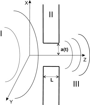
Figure 1:

The radiation sources are placed on the left of the screen, i.e., in the region $z<0$. We are concerned with the field produced by the source in space in the presence of the screen.

As we mentioned in the Introduction, a detailed analysis for a thin screen with a time-independent aperture radius was given in [3, 4] and generalized to the case with screen of thickness $L$ in [5]. Here we shall consider the case when the screen thickness is much less than the incident radiation wavelength. In this case, we can rule out that part of the volume which is occupied by region II with varying radius. Let us separately consider regions I and II that have an invariable volume. For these regions, the volume $V(t)$ and the surface $S(t)$ in (2) and (2) are time-independent. As a result, we can perform time integration over $t^{\prime}$ by parts in the right-hand side of the equation, and the integral equation for $\psi(\vec{r},t)$ takes a well-known form [1]:

$$\psi(\vec{r},t)=\int_{t_{0}}^{t_{1}}dt^{\prime}\int d^{3}r^{\prime}G(\vec{r},t;\vec{r}\,^{\prime},t^{\prime})f(\vec{r}\,^{\prime},t^{\prime})+$$

$$+ \frac{1}{4\pi c^{2}}\int d^{3}r^{\prime}\left.\left.\left(G(\vec{r},t;\vec{r}\,^{\prime},t_{0})\frac{\partial\psi(\vec{r}\,^{\prime},t^{\prime})}{\partial t^{\prime}}\right|_{t^{\prime}=t_{0}}-\psi(\vec{r}\,^{\prime},t_{0})\frac{\partial}{\partial t^{\prime}}G(\vec{r},t;\vec{r}\,^{\prime},t^{\prime})\right|_{t^{\prime}=t_{0}}\right)+$$

$$+ \frac{1}{4\pi}\int_{t_{0}}^{t_{1}}dt^{\prime}\int_{S}\left[G(\vec{r},t;\vec{r}\,^{\prime},t^{\prime})\frac{\partial\psi(\vec{r}\,^{\prime},t^{\prime})}{\partial n^{\prime}}-\psi(\vec{r}\,^{\prime},t^{\prime})\frac{\partial}{\partial n^{\prime}}G(\vec{r},t;\vec{r}\,^{\prime},t^{\prime})\right]dS^{\prime}.$$

For further consideration it will be useful to recall that Green’s function $G(\vec{r},t;\vec{r}\,^{\prime},t^{\prime})$ of wave equation (5) satisfies (7) and has the form

$$G(\vec{r},t;\vec{r}\,^{\prime},t^{\prime})=\frac{\delta\left(t-t^{\prime}-\frac{|\vec{r}-\vec{r}\,^{\prime}|}{c}\right)}{|\vec{r}-\vec{r}\,^{\prime}|}.$$ (12)

The presence of $\delta$ function in Green’s function enables us to perform time integration in (3), too. According to (3), the value of $\psi(\vec{r},t)$ at any point in the volume $V$ is defined by the function $f(\vec{r},t)$ of the source, the value of $\psi(r,t_{0})$, and $\left.\frac{\partial\psi(r,t)}{\partial t}\right|_{t=t_{0}}$ at the initial time, as well as by the value of $\psi(r,t)$ on the surface $S$ [1].

Let us consider (3) in region III on the right of the screen. No radiation source is placed in this region, and so there is no field present at the initial time.

Using the explicit expression for Green’s function, we can derive the following equation for $\psi(\vec{r},t)$ (for details, see [1]):

$$\psi(\vec{r},t)=$$

$$= \frac{1}{4\pi}\oint_{S}\vec{n}\left[\frac{1}{R}\vec{\nabla}_{\vec{r}\,^{\prime}}\psi(\vec{r}\,^{\prime},t^{\prime})-\frac{\vec{r}-\vec{r}\,^{\prime}}{|\vec{r}-\vec{r}\,^{\prime}|^{3}}\psi(\vec{r}\,^{\prime},t^{\prime})-\frac{\vec{r}-\vec{r}\,^{\prime}}{c|\vec{r}-\vec{r}\,^{\prime}|^{2}}\frac{\partial\psi(\vec{r}\,^{\prime},t^{\prime})}{\partial t^{\prime}}\right]_{{del}}dS^{\prime},$$

where $\left[...\right]_{del}$ indicates that after the derivatives are taken, $t^{\prime}$ is assumed to be the delay time $t^{\prime}=t-\frac{|\vec{r}-\vec{r}\,^{\prime}|}{c}$. Thus to find $\psi(\vec{r},t)$, we need to know $\psi$ and its derivative, which certainly, cannot be taken arbitrary [1], but requires the solution of the problem with given initial and boundary conditions.

Let a wave packet $\psi_{0}(\vec{r},t)$ be incident on the screen from the left (see Fig.):

$$\psi_{0}(\vec{r},t)=\int A(\vec{k}-\vec{k}_{0})e^{i\vec{k}\vec{r}}e^{-i\omega(k)t}d^{3}k.$$ (14)

When the characteristic wavelength $\lambda$ of the packet is much less than the aperture radius $a(t)$, following Kirchhoff, we shall assume that in the same way as in the stationary case, $\psi(\vec{r}\,^{\prime},t^{\prime})$ and $\frac{\partial\psi(\vec{r}\,^{\prime},t^{\prime})}{\partial t^{\prime}}$ equal zero on the surface of the screen in the region $z=0$ of screen location, while in the aperture $\psi(\vec{r}\,^{\prime},t^{\prime})=\psi_{0}(\vec{r}\,^{\prime},t^{\prime})$ and $\frac{\partial\psi(\vec{r}\,^{\prime},t^{\prime})}{\partial t^{\prime}}=\frac{\partial\psi_{0}(\vec{r}\,^{\prime},t^{\prime})}{\partial t^{\prime}}$. (To avoid confusion, hereafter the velocity $v$ of the aperture radius change is assumed to be $v\ll c$; below is shown how to consider the relativistic effects in diffraction of electromagnetic waves.)

As a result, at a large distance from the screen, $R\gg a$, equation (3) for the region on the right of the screen takes the form

$$\psi(\vec{r},t)=$$

$$= \frac{1}{4\pi}\int_{0}^{a({t^{\prime}_{a}})}\,\int^{2\pi}_{0}\rho^{\prime}d\rho^{\prime}d\varphi\,\vec{n}\left[\frac{1}{R}\vec{\nabla}_{\vec{r}\,^{\prime}}\psi_{0}(\vec{r}\,^{\prime},t^{\prime})-\frac{\vec{R}}{R^{3}}\psi_{0}(\vec{r}\,^{\prime},t^{\prime})-\frac{\vec{R}}{cR^{2}}\frac{\partial\psi_{0}(\vec{r}\,^{\prime},t^{\prime})}{\partial t^{\prime}}\right],$$

where $t^{\prime}_{a}=t-\frac{|\vec{r}-a(t_{a}^{\prime})|}{c}$.

Let us recall here that $R=|\vec{r}-\vec{r}\,^{\prime}|$ and $t^{\prime}=t-\frac{|\vec{r}-\vec{r}\,^{\prime}|}{c}$. We shall further consider $\psi(\vec{r},t)$ at a distance $r\gg a$ and discard the second term $\sim\frac{1}{R^{2}}$, leaving only the terms proportional to $\frac{1}{R}$.

Let us substitute (14) for $\psi_{0}(\vec{r},t)$ into (3). Now we have

$$\psi(\vec{r},t)=\int d^{3}kA(\vec{k}-\vec{k}_{0})\frac{1}{4\pi r}\int_{0}^{a({t^{\prime}_{a}})}\,\int^{2\pi}_{0}\rho^{\prime}d\rho^{\prime}d\varphi\,\vec{n}\left[i\vec{k}+i\frac{\omega(k)}{c}\vec{n}_{r}\right]e^{i\vec{k}\vec{r}^{\prime}}e^{-i\omega(k)t^{\prime}}$$

(16)

$$=-\frac{ik_{0}}{4\pi r}(1+\cos\vartheta)\int d^{3}\kappa A(\vec{\kappa})\int_{0}^{a({t^{\prime}_{a}})}\,\int^{2\pi}_{0}\rho^{\prime}d\rho^{\prime}d\varphi\left\{e^{i\vec{\kappa}\vec{\rho}\,^{\prime}}e^{+i\vec{k}_{0}\vec{\rho}\,^{\prime}}e^{-i\omega(\vec{k}_{0}+\vec{{\kappa}})t^{\prime}}\right\},$$

where $\vec{n}_{r}=\frac{\vec{r}}{r}$, $\vartheta$ is the angle between the $z$-axis and the direction of $\vec{r}$, and $t^{\prime}=t-\frac{|\vec{r}-\vec{r}\,^{\prime}|}{c}$.

Let us consider the diffraction of a quasi-monochromatic wave packet whose transverse dimensions are much greater than the aperture diameter and whose amplitude is, hence, almost constant in the aperture region. In this case ${\kappa_{0\perp}a\ll 1}$. Then we have

$$\psi(\vec{r},t)=-\frac{ik_{0}}{4\pi r}A\left(t-\frac{r}{c}\right)(1+\cos\vartheta)\int_{0}^{a({t^{\prime}_{a}})}\,\int_{0}^{2\pi}d^{2}\rho^{\prime}e^{-i(\vec{k}_{0}^{\prime}-\vec{k}_{0})\vec{\rho}\,^{\prime}}e^{ik_{0}r}e^{-i\omega_{0}t}$$

$$=\left(-\frac{ik_{0}}{4\pi}\right)(1+\cos\vartheta)\int_{0}^{a(t-\frac{r}{c})}\,\int_{0}^{2\pi}d^{2}\rho^{\prime}e^{-i(\vec{k}_{\perp}^{\prime}-\vec{k}_{0\perp})\vec{\rho}\,^{\prime}}\frac{e^{ik_{0}r}}{r}e^{-i\omega_{0}t}A\left(t-\frac{r}{c}\right)$$

$$=-\frac{ik_{0}}{4\pi}(1+\cos\vartheta)\int_{0}^{a(t-\frac{r}{c})}\rho^{\prime}d\rho^{\prime}d\varphi e^{-iq\rho\cos\varphi}A\left(t-\frac{r}{c}\right)\frac{e^{ik_{0}r}}{r}e^{-i\omega_{0}t},$$ (17)

$$\vec{q}=\vec{k}_{0\perp}^{\prime}-\vec{k}_{0\perp},\,\,q=|\vec{q}|.$$ (18)

We have

$$\psi(\vec{r},t)=-\frac{ik_{0}}{2}(1+\cos\vartheta)\int_{0}^{a(t-\frac{r}{c})}\rho d\rho J_{0}(q\rho)A\left(t-\frac{r}{c}\right)\frac{e^{ik_{0}r}}{r}e^{-i\omega_{0}t}$$ (19)

$$=-\frac{ik_{0}}{2}(1+\cos\vartheta)a\left(t-\frac{r}{c}\right)\frac{J_{1}[a{\left(t-\frac{r}{c}\right)}q]}{q}\frac{e^{ik_{0}r}}{r}e^{-i\omega_{0}t}A\left(t-\frac{r}{c}\right).$$

Let us recall that $t>\frac{r}{c}$.

Expression (19) for the wave diffracted by the aperture with a time-dependent radius includes the term $a\left(t-\frac{r}{c}\right)$ instead of $a$ appearing in the expression for $\psi(r,t)$, which describes wave diffraction by the aperture with invariable $a$. The same occurs in the case of diffraction by the additional screen: in formulas describing diffraction by the additional screen, the time-independent size is replaced by a time-dependent one. As a result, in the scalar theory the instantaneous output power radiated by the aperture per unit solid angle can be written in a form much similar to that for the stationary case (compare [1],[5])

$$\frac{dP}{d\Omega}=const\left[k_{0}a\left(t-\frac{r}{c}\right)\right]^{2}\left|\frac{J_{1}\left(a\left(t-\frac{r}{c}\right)q\right)}{a\left(t-\frac{r}{c}\right)q}\right|^{2}\left|A\left(t-\frac{r}{c}\right)\right|^{2},$$ (20)

$$q=|\vec{k}_{0\perp}^{\prime}-\vec{k}_{0\perp}|^{2}.$$

According to (19), the signal that has passed through the aperture appears to be modulated. Let us pay attention to the fact that for large $aq$, the Bessel functions are proportional to the sum of $\cos$ and $\sin$, i.e., they are proportional to $e^{\pm ia\left(t-\frac{r}{c}\right)q}$. If the radius $a(t-\frac{r}{c})$ increases at a constant rate $v_{a}$, then it follows from (19) that the function $\psi(\vec{r},t)$ appears the be proportional to $e^{i(r_{0}\pm\frac{v_{a}}{c}q)r}e^{-i(\omega_{0}\pm v_{a}q)t}$, and a shift in the frequency $\Delta\omega=\pm v_{q}q$ arises.

4 Diffraction by a sphere of radius $a(t)$

As another example we shall consider the diffraction of waves by a sphere of radius $a(t)$ undergoing radial contraction or expansion (Fig. 2).

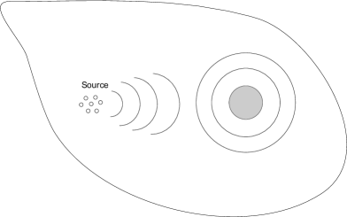
Figure 2:

According to the rules stated earlier in Section 2, in this case we can write (2) in the form:

$$\psi(\vec{r},t)-\int_{t_{0}}^{t_{1}}dt^{\prime}\int_{V_{sorce}}d^{3}r^{\prime}G(\vec{r},t;\vec{r}\,^{\prime}t^{\prime})f(\vec{r}\,^{\prime},t^{\prime})+$$

$$+ \frac{1}{4\pi c^{2}}\int d\Omega^{\prime}\int_{0}^{\infty}r^{\prime 2}dr^{\prime}\int_{t_{0}}^{t_{1}}dt^{\prime}\times$$

$$\times \left\{\Theta(r^{\prime}-a(t^{\prime}))G(\vec{r},t;\vec{r}\,^{\prime}t^{\prime})\frac{\partial^{2}\psi(\vec{r}\,^{\prime},t^{\prime})}{\partial t^{\prime 2}}-\Theta(r^{\prime}-a(t^{\prime}))\psi(\vec{r}\,^{\prime},t^{\prime})\frac{\partial^{2}G(\vec{r},t;\vec{r}\,^{\prime}t^{\prime})t}{\partial t^{2}}\right\}$$

$$= \frac{1}{4\pi}\int_{t_{0}}^{t_{1}}dt^{\prime}\int_{S(t^{\prime})}\left[G(\vec{r},t;\vec{r}\,^{\prime},t^{\prime})\frac{\partial\psi(\vec{r}\,^{\prime},t^{\prime})}{\partial n^{\prime}}-\psi(\vec{r}\,^{\prime},t^{\prime})\frac{\partial}{\partial n^{\prime}}G(\vec{r},t;\vec{r}\,^{\prime},t^{\prime})\right]dS^{\prime}.,$$

where $d\Omega^{\prime}$ denotes integration over the solid angle of vector $r\,^{\prime}$.

After partial integration of the third component on the left-hand side of (3), we have

$$\psi(\vec{r},t)=\int^{t_{1}}_{t_{0}}\int_{V_{source}}dt^{\prime}d^{3}r^{\prime}G(\vec{r},t;\vec{r}\,^{\prime}t^{\prime})f(\vec{r}\,^{\prime},t^{\prime})-$$

$$- \frac{1}{4\pi c^{2}}\int^{t_{1}}_{t_{0}}dt^{\prime}\int d\Omega^{\prime}a^{2}(t^{\prime})v(t^{\prime})\left(G\frac{\partial\psi}{\partial t^{\prime}}-\psi\frac{\partial G}{\partial t^{\prime}}\right)$$

$$+ \frac{1}{4\pi}\int^{t_{1}}_{t_{0}}dt^{\prime}\int d\Omega^{\prime}a^{2}(t^{\prime})\left\{G(\vec{r},t;\vec{r}\,^{\prime},t^{\prime})(\vec{n}\vec{\nabla}_{r^{\prime}})\psi(\vec{r}\,^{\prime},t^{\prime})-\psi(\vec{r}\,^{\prime},t^{\prime})(\vec{n}\vec{\nabla}_{r^{\prime}})G(\vec{r},t;\vec{r}\,^{\prime},t^{\prime})\right\},$$

where $v(t^{\prime})=\frac{da(t^{\prime})}{dt^{\prime}}$ is the velocity of sphere expansion (contraction).

Let us make use of the fact that [4]

$$G(\vec{r},t;\vec{r}\,^{\prime}t^{\prime})=\frac{\delta\left(t-t^{\prime}-\frac{R}{c}\right)}{R};$$

$$\vec{\nabla}_{r^{\prime}}G=\frac{(\vec{r}-\vec{r}\,^{\prime})}{|r-r^{\prime}|^{3}}\delta\left(t^{\prime}+\frac{R}{c}-t\right)-\frac{(\vec{r}-\vec{r}\,^{\prime})}{cR^{2}}\delta^{\prime}\left(t^{\prime}+\frac{R}{c}-t\right);$$

$\vec{R}=\vec{r}-\vec{r}\,^{\prime}$; here $\delta^{\prime}$ is the derivative of the $\delta$-function.

As a result, we have

$$\psi(\vec{r},t) = \psi_{source}+\frac{1}{4\pi}\int d\Omega^{\prime}a^{2}(t^{\prime})\left\{\frac{1}{|\vec{r}-\vec{r}(t^{\prime})|}\vec{n}\vec{\nabla}_{r^{\prime}}\psi(\vec{r}\,^{\prime},t^{\prime})\right.$$

$$- \left.\psi(\vec{r}\,^{\prime},t^{\prime})\frac{\vec{n}(\vec{r}-\vec{r}\,^{\prime})}{|\vec{r}-\vec{r}\,^{\prime}|^{3}}-\frac{\vec{n}(\vec{r}-\vec{r}\,^{\prime}(t^{\prime}))}{c|\vec{r}-\vec{r}\,^{\prime}(t^{\prime})|^{2}}\frac{\partial\psi(\vec{r},t^{\prime})}{\partial t^{\prime}}\right\}$$

$$- \frac{1}{4\pi}\int d\Omega\frac{\partial}{\partial t^{\prime}}\left\{a^{2}(t^{\prime})\frac{\vec{n}(\vec{r}-\vec{r}\,^{\prime}(t^{\prime}))}{c|\vec{r}-\vec{r}\,^{\prime}(t^{\prime})|^{2}}\right\}\psi(\vec{r}\,^{\prime},t^{\prime})$$

$$+ \frac{1}{2\pi c^{2}}\int d\Omega^{\prime}a^{2}(t^{\prime})v(t^{\prime})\frac{1}{|\vec{r}-\vec{r}\,^{\prime}(t^{\prime})|}\frac{\partial\psi}{\partial t^{\prime}}$$

$$+ \frac{1}{4\pi c^{2}}\int d\Omega^{\prime}\frac{1}{|\vec{r}-\vec{r}\,^{\prime}(t^{\prime})|}\frac{\partial}{\partial t^{\prime}}(a^{2}(t^{\prime})V(t^{\prime}))\psi(\vec{r}\,^{\prime},t^{\prime}).$$

At a large distance from the sphere (4) simplifies as follows

$$\psi(\vec{r},t)=\psi_{source}+\frac{1}{4\pi r}\int d\Omega^{\prime}a^{2}(t^{\prime})\left\{\vec{n}\vec{\nabla}_{r^{\prime}}\psi(\vec{r}\,^{\prime},t^{\prime})-\frac{\vec{n}\vec{n}_{r}}{c}\frac{\partial\psi(\vec{r}\,^{\prime},t^{\prime})}{\partial t^{\prime}}\right\}-$$ (24)

$$- \frac{\vec{n}\vec{n}_{r}}{2\pi cr}\int d\Omega^{\prime}a(t^{\prime})v(t^{\prime})\psi(\vec{r}\,^{\prime},t^{\prime})+\frac{1}{2\pi c^{2}r}\int d\Omega a^{2}(t^{\prime})v(t^{\prime})\frac{\partial\psi(\vec{r}\,^{\prime},t^{\prime})}{\partial t^{\prime}}+$$

$$+ \frac{1}{4\pi c^{2}r}\int d\Omega\frac{\partial}{\partial t^{\prime}}(a^{2}(t^{\prime}))v(t^{\prime}))\psi(\vec{r}\,^{\prime},t^{\prime}).$$

Thus, according to (4) and (24), the time-varying dimensions of the sphere lead to the appearance of additional terms (third, fourth, and fifth), whose amplitudes depend on the velocity $v$ and the acceleration of sphere expansion (contraction). The values of these additional contributions are proportional to the ratio of the velocity $v$ to the speed of light $c$. Because the power of the scattered wave $\psi_{sc}$ is proportional to $|\psi_{sc}|^{2}$, these additional contributions can be observed in studying the interference of the contributions to the intensity of scattered radiation that come from the product of the second and third (fourth or fifth) terms. At the same time, the contribution coming to the intensity from the additional terms themselves at $\frac{v}{c}\ll 1$ is small and can be omitted.

5 Vector analogue of the time-dependent Kirchhoff’s integral representation

Let us now proceed to the electromagnetic wave diffraction by a screen (aperture) with time-dependent dimensions. At first glance it may seem that because the electromagnetic field has a vector character, in this case only the coefficients appearing in (4)–(24) will change. But the situation appears to be more complicated, as due to relativistic effects, the magnetic field also makes a contribution to the strength of the electric field responsible for the current running in the moving screen. As a result, the contribution coming from the magnetic field to the process of electromagnetic field penetration through the screen can play an important, even critical role, for example, when an apertured screen is placed in the near-induction zone of the magnetic dipole.

To consider diffraction of the electromagnetic field in the case of time-dependent dimensions, we shall make use of the vector analogue of Green’s theorem [10]. Following [10], for vector analogue of Green’s theorem, we can write the relationship between the two vectors $\vec{P}$ and $\vec{F}$ in the form:

$$\int_{V}\left\{\vec{P}\cdot\vec{\nabla}^{2}\vec{F}-\vec{F}\cdot\vec{\nabla}^{2}\vec{P}\right\}d^{3}v$$

$$= \oint\left\{(\vec{P}\,{\texttt{div}}\,\vec{F}-\vec{F}\,{\texttt{div}}\,\vec{P})\cdot\vec{n}-(\vec{P}\cdot[\vec{n}\times\,{\texttt{rot}}\vec{F}]+\,{\texttt{rot}}\,\vec{P}\cdot[\vec{n}\times\vec{F}])\right\}ds,$$

where $\vec{n}$ is the external normal unit vector to the surface and

$\vec{\nabla}^{2}\vec{F}=\texttt{grad}\,\texttt{div}\,\vec{F}-\texttt{rot}\,\texttt{rot}\,\vec{F}$.

We shall further assume that vector $\vec{P}$ is the vector to be found, i.e., either the electric field strength $\vec{E}$ or the magnetic field strength $\vec{H}$. The Green function, which in the considered case is a tensor, is used for vector $\vec{F}$. The propagation of an electromagnetic wave in a free space is described by the vector Helmholtz equation [10]

$$\vec{\nabla}^{2}\vec{P}-\frac{1}{c^{2}}\frac{\partial^{2}\vec{P}}{\partial t^{2}}=-4\pi\vec{Q}_{P}(\vec{r},t).$$ (26)

The Green function is a symmetrical tensor $(\hat{G}\cdot\vec{P}=\vec{P}\cdot\hat{G})$ and has the form [10]

$$\vec{\nabla}^{2}\hat{G}(\vec{r},t;\vec{r}\,^{\prime}t^{\prime})-\frac{1}{c^{2}}\frac{\partial^{2}\hat{G}}{\partial t^{2}}=-4\pi\hat{I}\delta(\vec{r}-\vec{r}\,^{\prime})\delta(t-t^{\prime}),$$ (27)

where $\hat{I}$ is the unit operator.

Using (26) and (27), we can recast (5) as follows:

$$\int_{V(t)}\left\{\vec{P}{(\vec{r}\,^{\prime},t^{\prime})}\cdot\left(\frac{1}{c^{2}}\frac{\partial^{2}\hat{G}(\vec{r},t;\vec{r}\,^{\prime}t^{\prime})}{\partial t^{2}}-4\pi\hat{I}\delta(\vec{r}-\vec{r}^{\prime})\delta(t-t^{\prime})\right)-\right.$$

$$- \left.G(\vec{r},t;\vec{r}\,^{\prime}t^{\prime})\cdot\left(\frac{1}{c^{2}}\frac{\partial^{2}\vec{P}{(\vec{r}\,^{\prime},t^{\prime})}}{\partial t^{2}}-4\pi\vec{Q}(\vec{r}^{\prime},t^{\prime})\right)\right\}d^{3}V=$$

$$= \oint_{S(t^{\prime})}\left\{(\vec{P}\,\texttt{div}\,\hat{G}-\hat{G}\,\texttt{div}\,\vec{P})\cdot\vec{n}-(\vec{P}\cdot[\vec{n}\times\,{\texttt{rot}}\hat{G}]+\,{\texttt{rot}}\,\vec{P}\cdot[\vec{n}\times\hat{G}])\right\}ds,$$

Let us integrate (5) over the time $t^{\prime}$ between the limits from $t_{0}$ to $t_{1}>t$. As a result, we have the following integral equation for the vector field $\vec{P}(\vec{r},t)$ in the case of time-dependent $V(t)$ and $S(t)$ (let us recall that the retarded Green function $\hat{G}$ equals zero for $t^{\prime}>t$):

$$\vec{P}(\vec{r},t)=\int^{t_{1}}_{t_{0}}\int_{V_{(t^{\prime})}}\hat{G}(\vec{r},t;\vec{r}\,^{\prime}t^{\prime})\vec{Q}_{P}(\vec{r}\,^{\prime},t^{\prime})d^{3}vdt^{\prime}$$

$$- \frac{1}{4\pi c^{2}}\int^{t_{1}}_{t_{0}}\int_{V(t^{\prime})}\left(\hat{G}(\vec{r},t;\vec{r}\,^{\prime}t^{\prime})\frac{\partial^{2}\vec{P}(\vec{r}\,^{\prime},t^{\prime})}{\partial t^{\prime 2}}-\vec{P}(\vec{r}\,^{\prime},t^{\prime})\frac{\partial^{2}\hat{G}(\vec{r},t;\vec{r}\,^{\prime}t^{\prime})}{\partial t^{\prime 2}}\right)d^{3}r^{\prime}dt^{\prime}$$

$$- \frac{1}{4\pi}\int_{t_{0}}^{t_{1}}\oint_{S_{(}t^{\prime})}\left\{(\vec{P}\,\texttt{div}\,\hat{G}-\hat{G}\,\texttt{div}\,\vec{P})\cdot\vec{n}-(\vec{P}\cdot[\vec{n}\times\,{\texttt{rot}}\hat{G}]+\,{\texttt{rot}}\,\vec{P}\cdot[\vec{n}\times\hat{G}])\right\}ds,$$

Integral relation (5) generalizes the vector Kirchhoff’s integral representation with time-independent $V$ and $S$ to the case with time-dependent volume $V(t)$ and surface $S(t)$.

The integral relation (5) obtained here, as well as in the scalar case, can be used to find the fields $\vec{E}$ and $\vec{B}$ for the EM wave diffraction by an object (screen) with moving boundaries when the boundary conditions on the surface $S$ are fulfilled. In contrast to a static case, in the discussed case of moving boundaries account should be taken of the fact that relativistic effects mix the fields $\vec{E}$ and $\vec{B}$ on the surface $S$, making them dependent on the speed of the boundary motion.

The secondary waves appearing through diffraction are generated by those charges moving in the body which are set in motion by the Lorentz force that depends on both electric and magnetic components of the incident electromagnetic wave. In a weakly relativistic case, the currents $\vec{J}$ excited on the surface of the conducting body are proportional to $\vec{E}+\frac{1}{c}[\vec{v}(t)\vec{B}]$. As a result, for example, on the moving boundary of a high-conductivity metal, the tangential component of the effective electric field $(\vec{E}+\frac{1}{c}[\vec{v}(t)\vec{B}])_{t}$ equals zero rather than that of the electric field.

It is noteworthy that the vector analogue of time-dependent Kirchhoff’s integral representation, derived here, can be obtained from a scalar representation if by the field $\psi$ we understand the Cartesian components of the electric or magnetic field and then perform vector addition of the derived equations. However, thus obtained equations are inconvenient for further use, since the boundary conditions on the surface $S$ are difficult to satisfy, and therefore need modifying. To do this, we shall use the same approach as in deriving the vector analogue of Kirchhoff’s integral representation in the case of time-independent $V$ and $S$, given in [1].

For ease of treatment we further drop the additional terms appearing in (2) due to the varying dimensions of the screen that are proportional to $\frac{v}{c}$.

According to (2), in the scalar case the field $\psi(\vec{r},t)$ in the volume $V$ (in the absence of the sources inside $V$ and zero initial values of $\psi$ and $\frac{\partial\psi}{\partial t})$ is described by the expression of the form

$$\psi(\vec{r},t) = \frac{1}{4\pi}\int^{t1}_{t_{0}}dt^{\prime}\oint_{S(t^{\prime})}\left\{G(\vec{r},\vec{r}\,^{\prime},t,\vec{t}^{\prime})(\vec{n}\vec{\nabla}\,^{\prime})(\psi(\vec{r}\,^{\prime},t^{\prime})\right.$$

$$- \left.\psi(\vec{r}\,^{\prime},t^{\prime})(\vec{n}\vec{\nabla}^{\prime})G(\vec{r},\vec{r}\,^{\prime},t,t^{\prime})\right\}dS^{\prime}.$$

If by $\psi$ we understand a certain Cartesian component of the electric $\vec{E}$ or magnetic $\vec{B}$ field, then we can write

$$\vec{E}(\vec{r},t)=\frac{1}{4\pi}\int_{t_{0}}^{t_{1}}dt^{\prime}\oint_{S(t^{\prime})}\left\{G(\vec{n}\vec{\nabla}^{\prime})\vec{E}-\vec{E}(\vec{n}\vec{\nabla}^{\prime})G\right\}dS^{\prime}.$$ (31)

The integral over the surface converts to the form [1]

$$\oint_{S}\left\{G(\vec{n}\vec{\nabla}^{\prime})\vec{E}-\vec{E}(\vec{n}\vec{\nabla}^{\prime})G\right\}dS^{\prime}$$

$$= -\oint_{S}\left\{(\vec{n}\vec{E})\vec{\nabla}^{\prime}G+\left[[\vec{n}\times\vec{E}]\times\vec{\nabla}^{\prime}G\right]+G[\vec{n}\times rot^{\prime}\vec{E}]\right\}dS^{\prime}.$$

As a result, we have the following relationship:

$$\vec{E}(\vec{r},t) = -\frac{1}{4\pi}\int_{t_{0}}^{t_{1}}dt^{\prime}\oint_{S(t^{\prime})}\left\{\left(\vec{n}\vec{E}(\vec{r}\,^{\prime},t^{\prime})\right)\vec{\nabla}^{\prime}G+\left[[\vec{n}\times\vec{E}]\times\vec{\nabla}\,^{\prime}G\right]\right.$$

$$- \left.G\frac{1}{c}\left[\vec{n}\times\frac{\partial\vec{B}(\vec{r}\,^{\prime}t^{\prime})}{\partial t^{\prime}}\right]\right\}dS.$$

In a similar manner, we obtain for $\vec{B}$

$$\vec{B}(\vec{r},t) = -\frac{1}{4\pi}\int_{t_{0}}^{t_{1}}dt^{\prime}\oint_{S(t^{\prime})}\left\{\left(\vec{n}\vec{B}(\vec{r}\,^{\prime},t^{\prime})\right)\vec{\nabla}^{\prime}G+\left[[\vec{n}\times\vec{B}]\times\vec{\nabla}\,^{\prime}G\right]\right.$$

$$+ \left.G\frac{1}{c}\left[\vec{n}\times\frac{\partial\vec{E}(\vec{r}\,^{\prime}t^{\prime})}{\partial t^{\prime}}\right]\right\}dS^{\prime}.$$

Equations (5) and (5) derived here are a specific case of more generalized expressions (5), derived earlier in this section. Like (5), they are valid in the case when the surface $S$ is time-dependent, i.e., when $S=S(t^{\prime})$. For further transformations, let us make use of the fact that

$$\vec{\nabla}\,^{\prime}G(\vec{r},\vec{r}\,^{\prime};t,t^{\prime}) = -\frac{\vec{R}}{r}\frac{\partial}{\partial R}\left[\frac{\delta(t^{\prime}+\frac{R}{c}-t)}{R}\right]$$

$$= -\frac{\vec{R}}{R}\left\{-\frac{\delta(t^{\prime}+\frac{R}{c}-t)}{R^{2}}+\frac{\delta^{\prime}(t^{\prime}+\frac{R}{c}-t)}{cR}\right\}$$

$$= \frac{\vec{R}}{R^{3}}\delta(t^{\prime}+\frac{R}{c}-t)-\frac{\vec{R}}{cR^{2}}\delta^{\prime}(t^{\prime}+\frac{R}{c}-t).$$

Here $\vec{R}=\vec{r}-\vec{r}\,^{\prime}$.

As a result, we have

$$\vec{E}(\vec{r},t) = -\frac{1}{4\pi}\int_{t_{0}}^{t_{1}}dt^{\prime}\oint_{S(t^{\prime})}\left\{(\vec{n}\vec{E}(\vec{r}\,^{\prime},t^{\prime}))\left(\frac{\vec{R}}{R^{3}}\delta(t^{\prime}+\frac{R}{c}-t)-\frac{\vec{R}}{cR^{2}}\delta^{\prime}(t^{\prime}+\frac{R}{c}-t)\right)\right.$$ (36)

$$+ \left.\left[[\vec{n}\times\vec{E}]\times\left(\frac{\vec{R}}{R^{3}}\delta(t^{\prime}+\frac{R}{c}-t)-\frac{\vec{R}}{cR^{2}}\delta^{\prime}(t^{\prime}+\frac{R}{c}-t)\right)\right]\right.$$

$$- \left.\frac{1}{Rc}\delta(t^{\prime}+\frac{R}{c}-t)\left[\vec{n}\times\frac{\partial\vec{B}(\vec{r}\,^{\prime},t)}{\partial t^{\prime}}\right]\right\}ds.$$

Upon integration of (36) over time using $\delta$-function, we drop the terms proportional to $\frac{v}{c}$ and obtain the following equation

$$\vec{E}(\vec{r},t)=-\frac{1}{4\pi}\oint_{S(t^{\prime})}\left\{\frac{\vec{R}}{R^{3}}(\vec{n}\vec{E}(\vec{r}\,^{\prime},t^{\prime}))+\frac{\vec{R}}{cR^{2}}\frac{\partial}{\partial t^{\prime}}(\vec{n}\vec{E}(\vec{r}\,^{\prime},t^{\prime}))\right.$$

$$+ \left.\left[[\vec{n}\times\vec{E}]\times\frac{\vec{R}}{R^{3}}\right]+\frac{1}{c}\left[\left[\vec{n}\times\frac{\partial E}{\partial t^{\prime}}\right]\times\frac{\vec{R}}{R^{2}}\right]-\frac{1}{Rc}\left[\vec{n}\times\frac{\partial B(\vec{r}\,^{\prime},t^{\prime})}{\partial t^{\prime}}\right]\right\}ds.$$

Here $t^{\prime}=t-\frac{|\vec{r}-\vec{r}\,^{\prime}|}{c}$.

As $r\rightarrow\infty$, we can discard the terms proportional to $\frac{1}{R^{2}}$ and the integral over that part of the surface which is located a long distance away from the screen. In this case, we have

$$\vec{E}(\vec{r},t) = -\frac{1}{4\pi cr}$$

$$\times \oint_{S(t^{\prime})}\left\{\frac{\vec{r}}{r}\left(\vec{n}\frac{\partial\vec{E}(\vec{r}\,^{\prime}t^{\prime})}{\partial t^{\prime}}\right)+\left[\left[\vec{n}\times\frac{\partial\vec{E}}{\partial t^{\prime}}\right]\times\frac{\vec{r}}{r}\right]-\left[\vec{n}\times\frac{\partial\vec{B}}{\partial t^{\prime}}\right]\right\}ds.$$

Here $\vec{n}$ is the outer normal. If the normal is directed towards the observation area, the sign of the expression should be reversed. Then we have

$$\vec{E} = \frac{1}{4\pi cr}\oint_{S(t^{\prime})}\left\{\frac{\vec{r}}{r}\left(\vec{n}\frac{\partial\vec{E}}{\partial t^{\prime}}\right)+\left[\left[\vec{n}\times\frac{\partial\vec{E}}{\partial t}\right]\times\frac{\vec{r}}{r}\right]-\left[\vec{n}\times\frac{\partial\vec{B}}{\partial t^{\prime}}\right]\right\}ds,$$ (39)

$$t^{\prime} = t-\frac{R}{c}.$$

A similar to (39) expression for the magnetic field $\vec{B}(\vec{r},t)$ follows from (5):

$$\vec{B}=\frac{1}{4\pi cr}\oint_{S(t^{\prime})}\left\{\frac{\vec{r}}{r}\left(\vec{n}\frac{\partial\vec{B}}{\partial t^{\prime}}\right)+\left[\left[\vec{n}\times\frac{\partial\vec{B}}{\partial t^{\prime}}\right]\times\frac{\vec{r}}{r}\right]+\left[\vec{n}\times\frac{\partial\vec{E}(\vec{r}\,^{\prime},t^{\prime})}{\partial t^{\prime}}\right]\right\}ds.$$ (40)

For monochromatic fields $\vec{E}$, $\vec{B}$ $\sim e^{-i\omega t}$ and $t$-independent $S$, expression (36) converts to a well-known stationary expression (see formula (9.115) in [1]):

$$\vec{E}(\vec{r})=\frac{e^{ikr}}{4\pi ir}\oint_{S}\left\{\vec{k}(\vec{n}\vec{E}(\vec{r}\,^{\prime}))+\left[[\vec{n}\times\vec{E}]\times\vec{k}\right]-k[\vec{n}\times\vec{B}(\vec{r}\,^{\prime})]\right\}e^{-i\vec{k}\vec{r}\,^{\prime}}ds.\\$$ (41)

Let us recall that $\vec{k}=k\frac{\vec{r}}{r}$.

In a similar manner, we have for a magnetic field

$$\vec{B}=\frac{e^{ikr}}{4\pi ir}\oint\left\{\vec{k}(\vec{n}\vec{B}(\vec{r}\,^{\prime}))+\left[[\vec{n}\times\vec{B}]\times\vec{k}\right]+k[\vec{n}\times\vec{E}(\vec{r}\,^{\prime},\omega)]\right\}e^{-i\vec{k}\vec{r}\,^{\prime}}ds,$$ (42)

i.e.,

$$\vec{B}(\vec{r})=\frac{e^{ik\vec{r}}}{4\pi ir}\vec{k}\times\int_{S}\left[[[\vec{n}\times\vec{E}]\times\vec{n}_{r}]-[\vec{n}\times\vec{B}]\right]e^{-i\vec{k}\vec{r}\,^{\prime}}ds.$$ (43)

We shall also recall that

$$\vec{B}=\frac{1}{k}[\vec{k}\times\vec{E}].$$

Let a quasi-monochromatic wave packet be scattered by a perfectly conducting screen with dimensions much greater than the wavelength; the wave packet time length $T_{p}\gg\frac{L}{c}$, where $L$ is the characteristic dimension of the screen. In a similar manner as was done in the scalar case, we shall write the incident wave packet in the form:

$$\vec{E}_{in}(\vec{r},t)=\vec{E}_{0}\int A(\vec{k}-\vec{k}_{0})e^{i\vec{k}\vec{r}}e^{-i\omega t}d^{3}k.$$ (44)

Let us recall, that in view of the above, the motion of the screen boundary results in the appearance of the additional terms proportional to $\frac{v}{c}$ and $\frac{dv}{dt}$. These terms not only change the amplitudes of the fields but also lead to the electric field contribution to the magnetic field (and vice versa) due to relativistic effects.

In the beginning, we shall neglect these contributions. Let us recall that ${\omega_{0}\gg\frac{1}{T}}$, where $T$ is the characteristic time during which the speed of the screen changes. Using (44) and the boundary conditions on the screen surface [1], at a large distance from the screen we can obtain the following expression for the scattered fields $\vec{E}_{S}(\vec{r},t)$ and $\vec{B}_{S}(\vec{r},t)$:

$$\vec{E}_{S}(\vec{r},t) = \frac{e^{ikr}e^{-i\omega_{0}t}}{4\pi ir}A(r-ct)\times$$

$$\times \oint_{s(t^{\prime})}\left\{\vec{k}(\vec{n}\vec{E}_{0S})+\left[[\vec{n}\times\vec{E}_{0S}]\times\vec{k}\right]-k[\vec{n}\times\vec{B}_{0S}]\right\}e^{-i(\vec{k}-\vec{k}_{0})\vec{r}\,^{\prime}}ds,$$

where $\vec{B}_{S}=[\vec{n}_{k}\times\vec{E}_{S}]$, $\vec{k}=k_{0}\frac{\vec{r}}{r}$, and the fields (see[1]) $\vec{E}_{0S}\approx-\vec{E}_{0}$ and $\vec{B}_{0S}\approx-\vec{B}_{0}$ are in the shadow region of the obstacle. In the illuminated region of the obstacle, we have

$$\vec{n}\vec{E}_{0S}\simeq\vec{n}\vec{E}_{0},\,\,\vec{n}\times\vec{B}_{0S}=\vec{n}\times\vec{B}_{0},\,\,\vec{n}\times\vec{E}_{0S}=-\vec{n}\times\vec{E}_{0},$$ (46)

$$\vec{n}\vec{B}_{0S}=-\vec{n}\vec{B}_{0},\,\,\vec{B}=\frac{1}{k}[\vec{k}\times\vec{E}].$$

Using (41), we can write a similar expression for the magnetic field $\vec{B}(\vec{r},t)$

$$\vec{B}_{S}(\vec{r},t)=-\frac{i}{4\pi r}e^{ik_{0}r}e^{-i\omega_{0}t}A(r-ct)\times$$

$$\times \oint_{S(t^{\prime})}\left\{\vec{k}(\vec{n}\vec{B}_{0S})+\left[[\vec{n}\times\vec{B}_{0S}]\times\vec{k}\right]+k_{0}[\vec{n}\times\vec{E}_{0S}]\right\}e^{-i(\vec{k}-\vec{k}_{0})\vec{r}\,^{\prime}}ds,$$

i.e.,

$$\vec{B}(\vec{r},t)=\vec{F}_{B}\frac{e^{ik_{0}r}}{4\pi ir}e^{-iw_{0}t}A(r-ct)$$ (48)

where

$$\vec{F}_{B}=\vec{k}\times\vec{f}=e^{ik_{0}r}\vec{k}\times\oint_{S(t^{\prime})}\left\{\left[[\vec{n}\times\vec{E}_{0S}]\times\vec{n}_{k}\right]-[\vec{n}\times\vec{B}_{0S}]\right\}ds.$$ (49)

In a similar manner as in the scalar case, (5) and (50) can be obtained by substituting $S(t^{\prime})$ for $S$ in the expression describing scattering of a monochromatic wave by a screen with time-independent dimensions and then multiplying the expression by the amplitude $A(r-ct)$ of the wave packet.

As a result, in a similar manner as in the stationary case, from (5) we obtain, for example, the following expression for the electric field strength in the wave scattered at a small angle:

$$\vec{E}_{S}\approx ika^{2}(t^{\prime})\frac{I_{1}(ka(t^{\prime})\vartheta)}{ka(t^{\prime})\vartheta}\frac{e^{i(kr-\omega_{0}t)}}{r}\frac{(\vec{k}\times\vec{E}_{0})\times\vec{k}}{k^{2}}A(r-ct),$$ (50)

where $\vartheta$ is the scattering angle.

As we noted earlier, this contribution to field scattering can be obtained from the expression for the field in a stationary case [1]– [7] by substituting $a(t^{\prime})$ for $a$ and multiplying the expression for the field by the amplitude $A(r-ct)$ of the wave packet.

Let us recall that in deriving (5)–(39), we discarded the terms proportional to $\frac{v}{c}$ and to acceleration $\frac{dv}{dt}$. Similar to the scalar case, the contribution from these terms can be observed experimentally by studying the interference pattern of scattered radiation.

It is noteworthy that the additional terms can be divided into three groups. The first group includes the terms proportional to $\frac{v}{c}$ that only change the moduli of the fields. The second group comprises the terms proportional to the acceleration $\frac{dv}{dt}$, and the third one contains the terms admixing the magnetic field to the electric (or vice versa). Despite the smallness of $\frac{v}{c}$, the third group of terms is fundamentally important when the electric field itself is induced by the motion of the conductor in the magnetic field (i.e., electromagnetic induction).

In this case, the expressions for $\vec{E_{0}}$ and $\vec{B_{0}}$ in (46) should be rewritten for a relativistic case. For example, in a weakly relativistic case $\vec{E_{0}}$ converts to $\vec{E_{0}}+\frac{1}{c}[\vec{v}\vec{B_{0}}]$, and $\vec{B_{0}}$ to $\vec{B_{0}}-\frac{1}{c}[\vec{v}\vec{E_{0}}]$. If the field $\vec{E_{0}}$ is small, the rewritten expression for the initial fields includes $\vec{E_{0}}\simeq\frac{1}{c}[\vec{v}\vec{B_{0}}]$ and $\vec{B_{0}}=\vec{B_{0}}$.

Here we will not write cumbersome expressions describing the contribution to the intensity and the angular distribution of radiation that comes from the additional terms, leaving their detailed consideration for specific cases of practical importance.

6 Conclusion

We generalized Kirchhoff’s vector representation to the case of screens (apertures) with time-dependent dimensions. It has been shown that in the case when $\frac{v}{c}\ll 1$, the expressions for the scattered wave and instantaneous power can be derived from the appropriate expressions for a stationary case [1, 2, 3, 4, 5, 6] by substituting the time-dependent screen dimensions (e.g. time-dependent radius) for constant screen dimensions (e.g., the screen radius) appearing in the formulas describing the stationary case.

References

• [1] J. Jackson, Classical Electrodynamics (3rd ed.) New York: John Wiley & Sons, 1998.
• [2] S. Solimeno, B. Crosignani, P. DiPorto, Guiding, Diffraction and Confinement of Optical Radiation New York, Academic, 1986.
• [3] H. A. Bethe, Theory of Diffraction by Small Holes, Phys. Rev. Lett., Vol. 66 (1944) 153.
• [4] C. J. Bouwkamp, Diffraction Theory, Rep. Prog. Phys., Vol. 17 (1954) 35.
• [5] A. Yu. Nikitin, D. Zueco, F. J. Garcia-Vidal and L. Martin-Moreno, Electromagnetic wave transmission through a small hole in a perfect electric conductor of finite thickness, Phys. Rev. B Vol. 78 (2008) 165429.
• [6] S. Carretero-Palacios, F. J. Garcia-Vidal, L. Martin-Moreno, Sergio G. Rodrigo, Effect of film thickness and dielectric environment on optical transmission through subwavelength holes, Phys. Rev. B Vol. 85 (2012) 035417.
• [7] F. J. Garcia-Vidal, Esteban Moreno, J. A. Porto, L. Martin-Moreno, Transmission of light through a single rectangular hole, Phys.Rev. Lett. Vol. 95 (2005) 103901.
• [8] W.R. Morgans, The Kirchhoff formula extended to a moving surface, Philosophical Magazine, Vol. 9 (1930) 141.
• [9] F. Farassat, M. K. Myers, Extension of Kirchhoff’s formula to radiation from moving surfaces, Journal of Sound and Vibration, Vol. 123 (3) (1988) 451.
• [10] Ph. Morse and H. Feshbach, Methods of Theoretical Physics, Part 1, McGraw-Hill, 1953.