Fluctuations of the Euler-Poincaré characteristic
for random spherical harmonics

Abstract.

In this short note, we build upon recent results from [7] to present a precise expression for the asymptotic variance of the Euler-Poincaré characteristic for the excursion sets of Gaussian eigenfunctions on ${\cal S}^{2}$.

1. Introduction and main result

The geometry of excursion sets for Gaussian random fields has been a subject of intense research over the last fifteen years; much work has focussed on the investigation of the Euler-Poincaré characteristic, henceforth EPC [3]. We recall here that the EPC $\chi(A)$ is the unique integer-valued functional, defined on the ring $\mathcal{C}$ of closed convex sets in $\mathbb{R}^{N}$, which equals $\chi(A)=0$ if $A=\emptyset$, $\chi(A)=1$ if $A$ is homotopic to the unit ball, and satisfies the additivity property

$$\chi(A\cup B)=\chi(A)+\chi(B)-\chi(A\cap B),\hskip 28.45274pt\text{for all\;}A,B\in\mathcal{C}.$$

Clearly, the EPC is a topological invariant (i.e. it is invariant under homeomorphisms); its investigation for the excursion sets of random fields was initiated in the late seventies by Robert Adler and his co-authors. This stream of research has eventually resulted with the discovery of the beautiful Gaussian Kinematic Formula (GKF) [17, 2].

More precisely, let $f$ be a real valued random field defined on the parameter space $\mathcal{M}$; its excursion sets are defined as

$$A_{u}(f;{\mathcal{M}})=\left\{x\in{\mathcal{M}}:f(x)\geq u\right\},\hskip 28.45274ptu\in{\mathbb{R}}.$$

Let $\mathcal{L}^{f}_{j}$’s for $j=0,\dots,\text{dim}(\mathcal{M})$, denotes the Lipschitz-Killing curvatures for the manifold $\mathcal{M}$ with Riemannian metric $g^{f}$ induced by the covariance of $f$, i.e., for $U_{x},V_{x}\in T_{x}\mathcal{M}$, the tangent space to $\mathcal{M}$ at $x$ we have

$$g^{f}_{x}(U_{x},V_{x}):=\mathbb{E}[(U_{x}f)\cdot(V_{x}f)],$$

(see [2] for further details); in particular $\mathcal{L}_{0}$ is the EPC. The functions $\rho_{j}$’s are the so-called Gaussian Minkowski functionals and they are defined by

(1.1) $${\rho}_{j}(u)=(2\pi)^{-(j+1)/2}H_{j-1}(u)e^{-u^{2}/2},$$

where $H_{q}(\cdot)$ are the Hermite polynomial of order $q$:

$$H_{-1}(u)=1-\Phi(u),\hskip 28.45274ptH_{j}(u)=(-1)^{j}(\phi(u))^{-1}\frac{d^{j}}{du^{j}}\phi(u),\hskip 11.38092ptj=0,1,\dots,$$

$\phi(\cdot)$, $\Phi(\cdot)$ denote the standard Gaussian density and distribution functions, respectively; for example:

$$H_{0}(u)=1,\hskip 8.5359ptH_{1}(u)=u,\hskip 8.5359ptH_{2}(u)=u^{2}-1,\hskip 8.5359ptH_{3}(u)=u^{3}-3u,\dots$$

The GKF states that the expected EPC of the excursion sets of a smooth, centred, unit variance, Gaussian random fields $f:\mathcal{M}\to\mathbb{R}$ is

(1.2) $$\mathbb{E}[\chi(A_{u}(f;{\mathcal{M}}))]=\sum_{j=0}^{\text{dim}(\mathcal{M})}{\mathcal{L}}^{f}_{j}({\mathcal{M}}){\rho}_{j}(u).$$

While the GKF yields a precise expression for the expected value of the EPC of excursion sets of smooth Gaussian processes, the analysis of higher moments, and, in particular, of the variance, is still open. The latter question is of both theoretical and applied interest; for instance, in the recent paper [1] five different methods are suggested to estimate numerically the covariance matrix of the EPC characteristic for the joint excursion sets at various thresholds. These results were subsequently exploited to approximate excursion probabilities, the so-called Euler-Poincaré heuristic [3] Section 5.1.

In this paper, we establish analytic formulae for the covariance of the EPC characteristic of excursion sets at different thresholds, focussing on an important class of fields: Gaussian spherical harmonics. We establish a rather simple expression which seems to be closely related to a second-order Gaussian Kinematic formula, in a sense to be made clear below. More precisely, consider the Laplace equation

$$\Delta_{\mathcal{S}^{2}}f_{\ell}-\lambda_{\ell}f_{\ell}=0,\hskip 28.45274ptf_{\ell}:{\mathcal{S}}^{2}\to\mathbb{\mathbb{R}},$$

where $\Delta_{\mathcal{S}^{2}}$ is the Laplace-Beltrami operator on $\mathcal{S}^{2}$ and $\lambda_{\ell}=-\ell(\ell+1)$, $\ell=0,1,2,\dots$. For a given eigenvalue $\lambda_{\ell}$, the corresponding eigenspace is the $(2\ell+1)$-dimensional space of spherical harmonics of degree $\ell$; we can choose an arbitrary $L^{2}$-orthonormal basis $\left\{Y_{\mathbb{\ell}m}(.)\right\}_{m=-\ell,\dots,\ell}$, and consider random eigenfunctions of the form

$$f_{\ell}(x)=\frac{1}{\sqrt{2\ell+1}}\sum_{m=-\ell}^{\ell}a_{\ell m}Y_{\ell m}(x),$$

where the coefficients $\left\{a_{\mathbb{\ell}m}\right\}$ are independent, standard Gaussian variables. The law of $f_{\ell}$ is invariant w.r.t. the choice of a $L^{2}$-orthonormal basis $\{Y_{\ell m}\}$. The random fields $\{f_{\ell}(x),\;x\in\mathcal{S}^{2}\}$ are centred, Gaussian and isotropic, meaning that the probability laws of $f_{\ell}(\cdot)$ and $f_{\ell}(g\cdot)$ are the same for any rotation $g\in SO(3)$. From the addition theorem for spherical harmonics ([4] Theorem 9.6.3) the covariance function is given by

$$\mathbb{E}[f_{\ell}(x)f_{\ell}(y)]=P_{\ell}(\cos d(x,y)),$$

where $P_{\ell}$ are the Legendre polynomials and $d(x,y)$ is the spherical geodesic distance between $x$ and $y$. An application of the GKF (1.2) gives in these circumstances:

(1.3) $$\mathbb{E}[\chi(A_{u}(f_{\ell};{\mathcal{S}}^{2}))]=\frac{\sqrt{2}}{\sqrt{\pi}}\exp\{-u^{2}/2\}u\frac{\ell(\ell+1)}{2}+2[1-\Phi(u)],$$

for a proof of formula (1.3) see, for example, [10] Lemma 3.5 or [13] Corollary 5. Note that, as $u\to-\infty$, the right hand side of (1.3) yields the Euler-Poincaré characteristic of the two-dimensional sphere i.e.

$$\lim_{u\to-\infty}\mathbb{E}[\chi(A_{u}(f_{\ell};{\mathcal{S}}^{2}))]=2.$$

The analysis of spherical Gaussian eigenfunctions is motivated by applications arising mainly from Mathematical Physics and Cosmology. In particular, Gaussian eigenfunction have been conjectured [6] to approximate deterministic eigenfunctions on generic billiards (surfaces with smooth boundaries). On the other hand, spherical Gaussian eigenfunctions are the Fourier components of isotropic spherical random fields, and, because of this, have been deeply exploited in the analysis of cosmological data, see for instance [12].

Let $I\subseteq\mathbb{R}$ be any interval in the real line and

$$A_{I}(f_{\ell};\mathcal{S}^{2})=f_{\ell}^{-1}(I)=\left\{x\in\mathcal{S}^{2}:f_{\ell}(x)\in I\right\}.$$

Our principal result is the following:

Theorem 1.

As $\ell\to\infty$, for every intervals $I_{1},I_{2}\subseteq\mathbb{R}$,

(1.4) $${\rm Cov}[\chi(A_{I_{1}}(f_{\ell};{\cal S}^{2}))\,,\,\chi(A_{I_{2}}(f_{\ell};{\cal S}^{2}))]=\frac{\ell^{3}}{8\pi}{\cal I}_{1}{\cal I}_{2}+O(\ell^{5/2}),$$

where ${\cal I}_{i}$, for $i=1,2$, are given by

$${\cal I}_{i}=\int_{I_{i}}p(t_{i})dt_{i},\hskip 28.45274ptp(t)=(-t^{4}+4t^{2}-1)e^{-\frac{t^{2}}{2}}.$$

The constant involved in the $O(\cdot)$ notation is universal.

In particular the variance for any given interval follows as an easy corollary:

Corollary 1.

For every interval $I\subseteq\mathbb{R}$,

(1.5) $${\rm Var}[\chi(A_{I}(f_{\ell};{\cal S}^{2}))]=\frac{\ell^{3}}{8\pi}{\cal I}^{2}+O(\ell^{5/2})$$

where

$${\cal I}=\int_{I}(-t^{4}+4t^{2}-1)e^{-\frac{t^{2}}{2}}dt.$$

Note that the asymptotic covariance in (1.4) can be positive, negative or null depending on the choice of the intervals $I_{1}$ and $I_{2}$ (see Figure 1). From (1.4) and (1.5) it follows also that, for every intervals $I_{1},I_{2}\subseteq\mathbb{R}$ such that the corresponding variances do not vanish, as $\ell$ goes to infinity, $\chi(A_{I_{1}}(f_{\ell};\mathcal{S}^{2}))$ and $\chi(A_{I_{2}}(f_{\ell};\mathcal{S}^{2}))$ are asymptotically perfectly (positively or negatively) correlated, i.e.

Corollary 2.

For all intervals $I_{1},I_{2}$ such that

$${\rm Var}[\chi(A_{I_{1}}(f_{\ell};{\cal S}^{2}))],{\rm Var}[\chi(A_{I_{2}}(f_{\ell};{\cal S}^{2}))]\neq 0,$$

as $\ell\to\infty$,

$$|{\rm Corr}[\chi(A_{I_{1}}(f_{\ell};{\cal S}^{2}))\,,\,\chi(A_{I_{2}}(f_{\ell};{\cal S}^{2}))]|=1+O(\ell^{-1/2}).$$

A similar form of degeneracy was earlier observed for level curves in [19]. From Theorem 1 we also have the following corollary for half-intervals $I_{1}=[u_{1},\infty)$ and $I_{2}=[u_{2},\infty)$ (see also Figure 2 and Figure 3):

Corollary 3.

As $\ell\to\infty$, for $u_{1},u_{2}\in\mathbb{R}$,

(1.6) $${\rm Cov}[\chi(A_{u_{1}}(f_{\ell};{\cal S}^{2}))\,,\,\chi(A_{u_{2}}(f_{\ell};{\cal S}^{2}))]=\frac{\ell^{3}}{8\pi}u_{1}u_{2}(u_{1}^{2}-1)(u_{2}^{2}-1)e^{-\frac{u_{2}^{2}}{2}}e^{-\frac{u_{1}^{2}}{2}}+O(\ell^{5/2}).$$

In particular, if $u_{1}=u_{2}=u$, we can present an analytic expression for the variance:

(1.7) $${\rm Var}[\chi(A_{u}(f_{\ell};{\cal S}^{2}))] =\frac{\ell^{3}}{8\pi}[H_{3}(u)+2H_{1}(u)]^{2}e^{-u^{2}}+O(\ell^{5/2}),$$

where $H_{q}(\cdot)$ are the Hermite polynomial of order $q$.

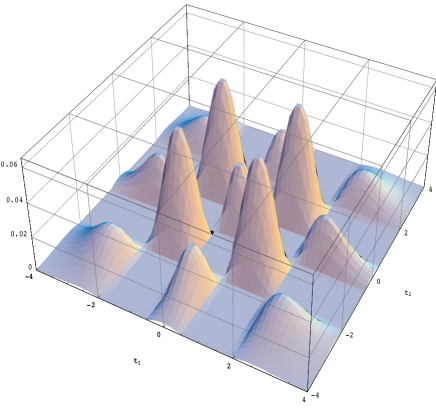
(a) positive range

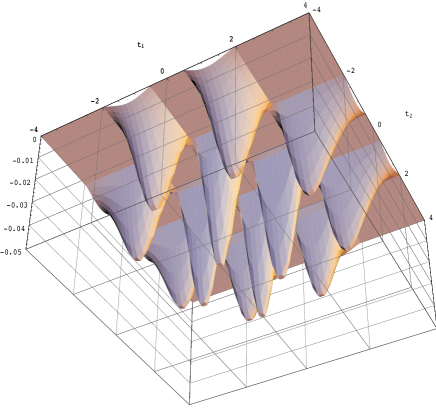
(b) negative range

Figure 1. $\frac{1}{8\pi}(-t_{1}^{4}+4t_{1}^{2}-1)(-t_{2}^{4}+4t_{2}^{2}-1)e^{-\frac{t_{1}^{2}}{2}}e^{-\frac{t_{2}^{2}}{2}}$

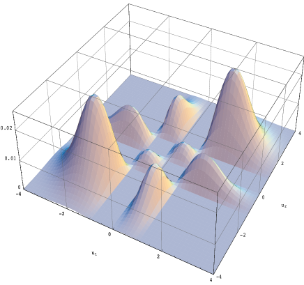
(a) positive range

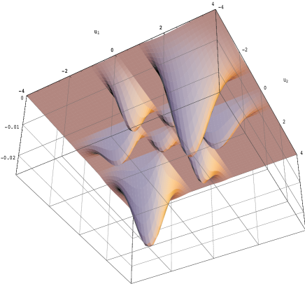
(b) negative range

Figure 2. $\frac{1}{8\pi}u_{1}u_{2}(u_{1}^{2}-1)(u_{2}^{2}-1)e^{-\frac{u_{1}^{2}}{2}}e^{-\frac{u_{2}^{2}}{2}}$

Figure 3. $\frac{1}{8\pi}[H_{3}(u)+2H_{1}(u)]^{2}e^{-u^{2}}$

As explained in Section 3, the proof of Theorem 1 follows from Morse theory and the analysis of asymptotic fluctuations of critical points of random eigenfunctions [7]. The expressions (1.4)-(1.7) are supported by extensive numerics [8].

Remark 2.

Building upon previous results [19], we are now able to present a full characterisation for the asymptotic behaviour for the variance of the three Lipschitz-Killing curvatures ${\cal L}_{i}$, $i=0,1,2$, for the excursion sets of random spherical eigenfunctions on ${\cal S}^{2}$. In this setting these three LKC’s correspond, respectively, to the EPC (${\cal L}_{0}$), half the length of level curves (${\cal L}_{1}$), and the excursion area (${\cal L}_{2}$). Indeed, it was shown [14] that the variance of the excursion area for spherical Gaussian eigenfunctions satisfies

(1.8) $$\lim_{\ell\to\infty}\ell\;{\rm Var}[{\cal L}_{2}(A_{u}(f_{\ell};{\cal S}^{2}))]=u^{2}\phi^{2}(u)=[H_{1}(u)+H^{\prime}_{0}(u)]^{2}\phi(u)^{2}.$$

On the other hand [19] formula (18) (see also [18]) asserts (in a slightly different form) that, for the variance of the boundary length of excursion sets, the following result holds

(1.9) $$\lim_{\ell\to\infty}\ell^{-1}{\rm Var}[{\cal L}_{1}(A_{u}(f_{\ell};{\cal S}^{2}))]={\rm const}\times u^{4}\phi^{2}(u)={\rm const}\times[H_{2}(u)+H^{\prime}_{1}(u)]^{2}\phi^{2}(u).$$

Likewise the asymptotic variance of the Euler-Poincaré characteristic, derived in Corollary 3, may be written as

(1.10) $$\lim_{\ell\to\infty}\ell^{-3}{\rm Var}[{\cal L}_{0}(A_{u}(f_{\ell};{\cal S}^{2}))]=\frac{1}{4}[u^{3}-u]^{2}\phi^{2}(u)=\frac{1}{4}[H_{3}(u)+H^{\prime}_{2}(u)]^{2}\phi^{2}(u).$$

We may unite the asymptotic expressions for the variance of the first three Lipschitz-Killing curvatures in (1.8), (1.9) and (1.10) into a single formula:

(1.11) $$\lim_{\ell\to\infty}\ell^{2k-3}\times{\rm Var}[{\cal L}_{k}(A_{u}(f_{\ell};{\cal S}^{2})]=const\times[H_{3-2k}(u)+H^{\prime}_{2-2k}(u)]^{2}\;\phi^{2}(u),\hskip 14.22636ptk=0,1,2.$$

A comparison of (1.11) with expressions (1.1), (1.2) and (1.3) seems to suggest the existence of an (asymptotic) second order Gaussian Kinematic Formula for spherical Gaussian eigenfunctions. We leave the investigation of the general validity of such en expression for higher dimensional spheres to future research.

Remark 3.

For all $u\in\mathbb{R}$, we have

$$\frac{\chi(A_{u}(f_{\ell};{\cal S}^{2}))}{\mathbb{E}[\chi(A_{u}(f_{\ell};{\cal S}^{2}))]}-1=O_{p}\Big{(}\frac{1}{\sqrt{\ell}}\Big{)},$$

with the usual convention $X_{n}=O_{p}(a_{n})$ meaning that the sequence $|X_{n}|/a_{n}$ is bounded in probability; i.e., in the high frequency limit $\ell\rightarrow\infty$, the ratio of the realised and expected value for the EPC of the excursion will converge to unity in probability for all $u\in\mathbb{R}$.

2. Background on Morse theorem and (approximate) Kac-Rice formula

2.1. Morse theorem

We start by recalling a general expression for the EPC by means of so-called Morse Theorem (see [2] Section 9.3). Assuming that $\mathcal{M}$ is a $C^{2}$ manifold without boundary in $\mathbb{R}^{N}$ and that $h\in C^{2}(\mathcal{M})$ is a Morse function on $\mathcal{M}$ (i.e. its Hessian is non degenerate at the critical points), we have

(2.1) $$\chi({\mathcal{M}})=\sum_{j=0}^{\text{dim}(\mathcal{M})}(-1)^{j}\mu_{j}({\mathcal{M}},h),$$

where $\mu_{j}(\mathcal{M},h)$ is the number of critical points of $h$ with Morse index $j$, i.e., the Hessian of $h$ has $j$ negative eigenvalues. In order to develop our results we will need to exploit (2.1) in the case of excursion sets of spherical eigenfunctions; to this end, let us first recall some basic differential geometry on $\mathcal{S}^{2}$. The metric tensor on the tangent plane $T(\mathcal{S}^{2})$ is given by

$$g(\theta,\varphi)=\left[\begin{matrix}1&0\\ 0&\sin^{2}\theta\end{matrix}\right].$$

For $x=(\theta,\varphi)\in\mathcal{S}^{2}\setminus\{N,S\}$ ($N,S$ are the north and south poles i.e. $\theta=0$ and $\theta=\pi$ respectively), the vectors

$$\vec{e}_{\theta}=\frac{\partial}{\partial\theta},\hskip 56.9055pt\vec{e}_{\varphi}=\frac{1}{\sin\theta}\frac{\partial}{\partial\varphi},$$

constitute an orthonormal basis for $T_{x}(\mathcal{S}^{2})$; in these coordinates the gradient is given by $\nabla=(\frac{\partial}{\partial\theta},\frac{1}{\sin\theta}\frac{\partial}{\partial\varphi})$. The Hessian of a function $f\in C^{2}(\mathcal{S}^{2})$ is the bilinear symmetric map from $C^{1}(T(\mathcal{S}^{2}))\times C^{1}(T(\mathcal{S}^{2}))$ to $C^{0}(\mathcal{S}^{2})$ defined by

$$\nabla^{2}f(X,Y)=XYf-\nabla_{X}Yf,\hskip 28.45274ptX,Y\in T(\mathcal{S}^{2}),$$

where $\nabla_{X}$ denotes Levi-Civita connection (see e.g. [2] Chapter 7 for more discussion and details). For our computations to follow we shall need the matrix-valued process $\nabla^{2}_{E}{f_{\ell}}(x)$ with elements given by

$$\{\nabla^{2}_{E}{f_{\ell}}(x)\}_{a,b=\theta,\varphi}=\{(\nabla^{2}{f_{\ell}}(x))(\vec{e}_{a},\vec{e}_{b})\}_{a,b=\theta,\varphi},$$

where $E=\{\vec{e}_{\theta},\vec{e}_{\varphi}\}$. In coordinates as above, this matrix can be expressed as

$$\nabla^{2}_{E}f_{\ell}(x) =\left[\begin{matrix}\frac{\partial^{2}}{\partial\theta^{2}}-\Gamma^{\theta}_{\theta\theta}\frac{\partial}{\partial\theta}-\Gamma^{\varphi}_{\theta\theta}\frac{\partial}{\partial\varphi}&\frac{1}{\sin\theta}[\frac{\partial^{2}}{\partial\theta\partial\varphi}-\Gamma^{\varphi}_{\varphi\theta}\frac{\partial}{\partial\varphi}-\Gamma^{\theta}_{\theta\varphi}\frac{\partial}{\partial\theta}]\\ \frac{1}{\sin\theta}[\frac{\partial^{2}}{\partial\theta\partial\varphi}-\Gamma^{\varphi}_{\varphi\theta}\frac{\partial}{\partial\varphi}-\Gamma^{\theta}_{\theta\varphi}\frac{\partial}{\partial\theta}]&\frac{1}{\sin^{2}\theta}[\frac{\partial^{2}}{\partial\varphi^{2}}-\Gamma^{\varphi}_{\varphi\varphi}\frac{\partial}{\partial\varphi}-\Gamma^{\theta}_{\varphi\varphi}\frac{\partial}{\partial\theta}]\end{matrix}\right]$$

$$=\left[\begin{matrix}\frac{\partial^{2}}{\partial\theta^{2}}&\frac{1}{\sin\theta}[\frac{\partial^{2}}{\partial\theta\partial\varphi}-\frac{\cos\theta}{\sin\theta}\frac{\partial}{\partial\varphi}]\\ \frac{1}{\sin\theta}[\frac{\partial^{2}}{\partial\theta\partial\varphi}-\frac{\cos\theta}{\sin\theta}\frac{\partial}{\partial\varphi}]&\frac{1}{\sin^{2}\theta}[\frac{\partial^{2}}{\partial\varphi^{2}}+\sin\theta\cos\theta\frac{\partial}{\partial\theta}]\end{matrix}\right].$$

Here $\Gamma_{ab}^{c}$ are the usual Christoffel symbols, see e.g. [9] Section I.1, which allow to compute the Levi-Civita connection:

$$\nabla_{\vec{e}_{a}}\vec{e}_{b}=\Gamma_{ab}^{\theta}\vec{e}_{\theta}+\Gamma_{ab}^{\varphi}\vec{e}_{\varphi},\hskip 19.91684pta,b=\theta,\varphi.$$

More explicitly, Christoffel symbols for $\mathcal{S}^{2}$ are given by

$$\Gamma^{\theta}_{\theta\varphi}=\Gamma^{\theta}_{\theta\theta}=\Gamma^{\varphi}_{\varphi\varphi}=\Gamma^{\varphi}_{\theta\theta}=0,\hskip 14.22636pt\Gamma_{\varphi\varphi}^{\theta}=-\sin\theta\cos\theta,\hskip 14.22636pt\Gamma_{\varphi\theta}^{\varphi}=\cot\theta.$$

We now state the Morse representation for the Euler characteristic of the excursion set: let $\mathcal{M}$ and $h$ in (2.1) be $A_{I}(f_{\ell};\mathcal{S}^{2})$ and $\left.f_{\ell}\right|_{{A_{I}(f_{\ell};\mathcal{S}^{2})}}$ respectively, we have

(2.2) $$\chi(A_{I}(f_{\ell};{\mathcal{S}}^{2}))=\sum_{j=0}^{2}(-1)^{j}\mu_{j},$$

where

$$\mu_{j}=\#\{x\in{\mathcal{S}}^{2}:f_{\ell}(x)\in I,\nabla f_{\ell}(x)=0,\text{Ind}(-\nabla^{2}_{E}f_{\ell}(x))=j\},$$

$\text{Ind}(M)$ denoting the number of negative eigenvalues of a square matrix $M$. More specifically, $\mu_{0}$ is the number of maxima, $\mu_{1}$ the number of saddles, and $\mu_{2}$ the number of minima in the excursion region $A_{I}(f_{\ell};\mathcal{S}^{2})$.

2.2. Kac-Rice formula

The Kac-Rice formula is a standard tool (or meta-theorem) for expressing the (factorial) moments of the zero crossings number of a Gaussian process in terms of certain explicit integrals. In our case, we are interested in counting the critical points of $f_{\ell}$, i.e. the zeros of the map $x\rightarrow\nabla f_{\ell}(x)$. Let $\mathcal{E}\subset\mathbb{R}^{n}$ be a nice Euclidean domain, and $g:\mathcal{E}\rightarrow\mathbb{R}^{n}$ a centred Gaussian random field, a.s. smooth. Define the $2$-point correlation function of critical points $K_{2}=K_{2;g}:\mathcal{E}^{2}\rightarrow\mathbb{R}$

$$K_{2}(x,y)=\phi_{(\nabla g(x),\nabla g(y))}(\mathbf{0},\mathbf{0})\cdot\mathbb{E}[|\mathrm{det}\nabla^{2}g(x)|\cdot|\mathrm{det}\nabla^{2}g(y)|\big{|}\nabla g(x)=\nabla g(y)=\mathbf{0}],$$

where $\phi_{(\nabla g(x),\nabla g(y))}$ is the Gaussian probability density of $(\nabla g(x),\nabla g(y))\in\mathbb{R}^{2n}$. Let $\mathcal{N}^{c}(g)=\mathcal{N}^{c}(g,\mathcal{E})=\#\{x\in\mathcal{E}:\nabla g(x)=\mathbf{0}\}$; by virtue of [5] Theorem 6.3, we have

$$\mathbb{E}[{\mathcal{N}}^{c}(g,{\mathcal{E}})\cdot({\mathcal{N}}^{c}(g,{\mathcal{E}})-1)]=\iint_{\mathcal{E}\times\mathcal{E}}K_{2}(x,y)dxdy,$$

provided that the Gaussian distribution of $\left(\nabla g(x),\nabla g(y)\right)\in\mathbb{R}^{2n}$ is non-degenerate for all $(x,y)\in\mathcal{E}^{2}$, on the validity condition of Kac-Rice formula in the Gaussian case, see [5] Theorem 6.3 and Proposition 1.2, and [16] Section 1.4. Moreover for $\mathcal{D}_{1},\mathcal{D}_{2}\subseteq\mathcal{E}$ two nice disjoint domains, under the same non-degeneracy assumptions for every $(x,y)\in\mathcal{D}_{1}\times\mathcal{D}_{2}$, we have

$$\mathbb{E}[{\mathcal{N}}^{c}(g,{\mathcal{D}}_{1})\cdot{\mathcal{N}}^{c}(g,{\mathcal{D}}_{2})]=\iint_{\mathcal{D}_{1}\times\mathcal{D}_{2}}K_{2}(x,y)dxdy.$$

It is easy to adapt the definition of the $2$-point correlation function in order to investigate, for example, the maxima with values lying in an interval $I\subseteq\mathbb{R}$: we re-define $K_{2}$ as

$$K_{2,0,0}(x,y;I,I)=\phi_{(\nabla g(x),\nabla g(y))}(\mathbf{0},\mathbf{0})$$

$$\times\mathbb{E}[|\mathrm{det}\nabla^{2}g(x)|\cdot|\mathrm{det}\nabla^{2}g(y)|\cdot 1\mbox{\rm l}_{I}(g(x))\cdot 1\mbox{\rm l}_{I}(g(y))\cdot 1\mbox{\rm l}_{\{\text{Ind}(-\nabla^{2}g(x))=0\}}\cdot 1\mbox{\rm l}_{\{\text{Ind}(-\nabla^{2}g(y))=0\}}\big{|}\nabla g(x)=\nabla g(y)=\mathbf{0}],$$

where $1\mbox{\rm l}_{I}$ is the characteristic function of $I$ on $\mathbb{R}$.

For the Kac-Rice formula on manifolds we refer to [2] Theorem 12.1.1, in particular, let

$$\mathcal{N}_{I}^{c}(f_{\ell})=\#\{x\in\mathcal{S}^{2}:\;f_{\ell}(x)\in I,\nabla f_{\ell}(x)=0\}$$

be the total number of critical points in $I$ of $\{f_{\ell}(x),x\in\mathcal{S}^{2}\}$; we have

(2.3) $$\mathbb{E}[\mathcal{N}_{I}^{c}(f_{\ell})\cdot(\mathcal{N}_{I}^{c}(f_{\ell})-1)]=\iint\limits_{\mathcal{S}^{2}\times\mathcal{S}^{2}}K_{2,\ell}(x,y;I,I)dxdy,$$

where

$$K_{2,\ell}(x,y;I,I) =\phi_{(\nabla f_{\ell}(x),\nabla f_{\ell}(y))}(\mathbf{0},\mathbf{0})$$

(2.4) $$\;\;\times\mathbb{E}[|\det\nabla_{E}^{2}f_{\ell}(x)|\cdot|\det\nabla_{E}^{2}f_{\ell}(y)|\cdot 1\mbox{\rm l}_{I}(f_{\ell}(x))\cdot 1\mbox{\rm l}_{I}(f_{\ell}(y))\big{|}\nabla f_{\ell}(x)=\nabla f_{\ell}(y)=\mathbf{0}].$$

One technical difficulty in working with the spherical Gaussian eigenfunctions $f_{\ell}$ in (2.3) is related to the fact that the Gaussian distribution of $(f_{\ell}(x),\nabla f_{\ell}(x),\nabla_{E}^{2}f_{\ell}(x))$ is always degenerate. However, this issue can be handled by writing $f_{\ell}$ as a linear combination of second order derivatives, and thus reducing the dimension of the Gaussian vector involved in the evaluation of $K_{2}$, see [7].

A much trickier issue arises when we need to validate a sufficient non-degeneracy assumptions due to the technical difficulties of dealing with $10\times 10$ matrices depending on both $x$ and $y$ (and $\ell$). Following [7] and [15], we do not claim the (precise) Kac-Rice formula (2.3) but rather an approximate version, see [7] formula (3.5), equivalent to (2.3) up to an admissible error.

First note that, by isotropy, $K_{2}(x,y)=K_{2}(d(x,y))$ depends only on the (spherical) distance $d(x,y)=\arccos(\left\langle x,y\right\rangle)$ between $x$ and $y$. In view of this, we note that it is convenient to perform our computations along a specific geodesic; in particular, we constrain ourselves to the equatorial line $\theta_{x}=\theta_{y}=\pi/2$; it is immediate to see that here the gradient and the Hessian are

$$\left.\nabla\right|_{\theta=\pi/2}=(\frac{\partial}{\partial\theta},\frac{\partial}{\partial\varphi}),\hskip 28.45274pt\left.\nabla^{2}_{E}\right|_{\theta=\pi/2}=\left[\begin{matrix}\frac{\partial^{2}}{\partial\theta^{2}}&\frac{\partial^{2}}{\partial\theta\partial\varphi}\\ \frac{\partial^{2}}{\partial\theta\partial\varphi}&\frac{\partial^{2}}{\partial\varphi^{2}}\end{matrix}\right].$$

The basic idea is to split the range of integration in (2.3) into two parts: the “short range” regime $d(x,y)<C/\ell$ and the “long range” regime $d(x,y)>C/\ell$, $C$ denoting a sufficiently big positive constant. In the short range regime Kac-Rice formula holds only approximately, but, by a partitioning argument inspired from [15] (see also [18]), it is possible to prove that its contribution is $O(\ell^{2})$. In the long range regime $d(x,y)>C/\ell$ the Kac-Rice formula is precise. The above yields

(2.5) $$\mathbb{E}[\mathcal{N}_{I}^{c}(f_{\ell})\cdot(\mathcal{N}_{I}^{c}(f_{\ell})-1)]=\int_{d(x,y)>C/\ell}\iint_{I\times I}K_{2,\ell}(x,y;t_{1},t_{2})dt_{1}dt_{2}dxdy+O(\ell^{2}),$$

where

(2.6) $$K_{2,\ell}(x,y;t_{1},t_{2})$$

$$\;\;=\varphi_{x,y,\ell}(t_{1},t_{2},\mathbf{0},\mathbf{0})\mathbb{E}[|\det\nabla_{E}^{2}f_{\ell}(x)|\cdot|\det\nabla^{2}_{E}f_{\ell}(y)|\big{|}\nabla f_{\ell}(x)=\nabla f_{\ell}(y)=\mathbf{0},f_{\ell}(x)=t_{1},f_{\ell}(y)=t_{2}],$$

and $\varphi_{x,y,\ell}$ is the density of the $6$-dimensional vector $(f_{\ell}(x),f_{\ell}(y),\nabla f_{\ell}(x),\nabla f_{\ell}(y))$. For further details on the proof of (2.5), see [7] Section 3.4.1 and Section 3.4.2.

As it will become clear from the proof of Proposition 2 below, we obtain a considerable simplification in our calculations since, during the application of the (approximate) Kac-Rice formula for studying the variance of the EPC, we can get rid of the absolute values in (2.6); in fact, for $g$ as before a smooth, centred Gaussian random field, we observe that ([3] Lemma 4.2.2)

$$(-1)^{j}\;|\det\nabla_{E}^{2}g(x)|1\mbox{\rm l}_{\{\text{Ind}(-\nabla_{E}^{2}g(x))=j\}} =(-1)^{j}\;\text{sgn}(\det\nabla_{E}^{2}g(x))(\det\nabla_{E}^{2}g(x))1\mbox{\rm l}_{\{\text{Ind}(-\nabla_{E}^{2}g(x))=j\}}$$

$$=\det(-\nabla_{E}^{2}g(x))1\mbox{\rm l}_{\{\text{Ind}(-\nabla_{E}^{2}g(x))=j\}},$$

since $\text{sgn}(\det\nabla_{E}^{2}g(x))1\mbox{\rm l}_{\{\text{Ind}(-\nabla_{E}^{2}g(x))=j\}}=(-1)^{j+1}$ and $-\det\nabla_{E}^{2}g(x)=\det(-\nabla_{E}^{2}g(x))$. Hence

(2.7) $$\sum_{j=0}^{2}(-1)^{j}\;|\det\nabla_{E}^{2}g(x)|1\mbox{\rm l}_{\{\text{Ind}(-\nabla_{E}^{2}g(x))=j\}}=\det(-\nabla_{E}^{2}g(x)).$$

3. Proof of Theorem 1

Let $I_{i}\subseteq\mathbb{R}$, $i=1,2$ be two interval in the real line; in the argument to follow we shall adopt the following notation:

$$\mu_{j;i}(f_{\ell})=\#\{x\in{\mathcal{S}}^{2}:f_{\ell}(x)\in I_{i},\nabla f_{\ell}(x)=0,\text{Ind}(-\nabla_{E}^{2}f_{\ell}(x))=j\},\hskip 28.45274ptj=0,1,2,\;i=1,2.$$

Theorem 1 is a straightforward application of Proposition 1 and Proposition 2. The first building block is the approximate Kac-Rice formula for covariance computation:

Proposition 1.

There exists a constant $C>0$ sufficiently big, such that

(3.1) $$\sum_{j,k=0}^{2}(-1)^{j+k}\mathbb{E}[\mu_{j;1}(f_{\ell})\mu_{k;2}(f_{\ell})]=\int_{d(x,y)>C/\ell}\iint_{I_{1}\times I_{2}}{J}_{2,\ell}(x,y;t_{1},t_{2})dt_{1}dt_{2}dxdy+O(\ell^{2})$$

where

(3.2) $${J}_{2,\ell}(x,y;t_{1},t_{2})$$

$$\;\;=\varphi_{x,y,\ell}(t_{1},t_{2},{\bf 0},{\bf 0})\;\mathbb{E}[\det(-\nabla_{E}^{2}f_{\ell}(x))\cdot\det(-\nabla_{E}^{2}f_{\ell}(y))\big{|}\nabla f_{\ell}(x)=\nabla f_{\ell}(y)={\bf 0},f_{\ell}(x)=t_{1},f_{\ell}(y)=t_{2}].$$

Proof.

We start by observing that

(3.3) $$\sum_{j,k=0}^{2}(-1)^{j+k}\mathbb{E}[\mu_{j;1}(f_{\ell})\mu_{k;2}(f_{\ell})]=\sum_{j\neq k}(-1)^{j+k}\mathbb{E}[\mu_{j;1}(f_{\ell})\mu_{k;2}(f_{\ell})]+\sum_{j=0}^{2}\mathbb{E}[\mu_{j;1}(f_{\ell})\mu_{j;2}(f_{\ell})].$$

For the non diagonal terms in (3.3) with $j\neq k$, $j,k=0,1,2$, we directly obtain (see [7] Section 3.4) that for any sufficiently big constant $C>0$, we have

$$\mathbb{E}[\mu_{j;1}(f_{\ell})\mu_{k;2}(f_{\ell})]=\int_{d(x,y)>C/\ell}\iint_{I_{1}\times I_{2}}\tilde{K}_{2,\ell,j,k}(x,y;t_{1},t_{2})dt_{1}dt_{2}dxdy+O(\ell^{2}),$$

where

$$\tilde{K}_{2,\ell,j,k}(x,y;t_{1},t_{2}) =\varphi_{x,y,\ell}(t_{1},t_{2},\mathbf{0},\mathbf{0})$$

$$\times\mathbb{E}[|\det\nabla_{E}^{2}f_{\ell}(x)|\cdot|\det\nabla_{E}^{2}f_{\ell}(y)|\cdot 1\mbox{\rm l}_{\{\mathrm{Ind}(-\nabla_{E}^{2}f_{\ell}(x))=j\}}\cdot 1\mbox{\rm l}_{\{\mathrm{Ind}(-\nabla_{E}^{2}f_{\ell}(y))=k\}}\big{|}\nabla f_{\ell}(x)=\nabla f_{\ell}(y)=\mathbf{0},f_{\ell}(x)=t_{1},f_{\ell}(y)=t_{2}].$$

To work out the diagonal terms $\mathbb{E}[\mu_{j;1}(f_{\ell})\mu_{j;2}(f_{\ell})]$, $j=0,1,2$, in (3.3), we introduce the following notation:

$$\mu_{j;i\setminus i^{\prime}}(f_{\ell}) =\#\{x\in{\mathcal{S}}^{2}:f_{\ell}(x)\in I_{i}\setminus I_{i^{\prime}},\nabla f_{\ell}(x)=0,\text{Ind}(-\nabla_{E}^{2}f_{\ell}(x))=j\},$$

$$\mu_{j;i\cap i^{\prime}}(f_{\ell}) =\#\{x\in{\mathcal{S}}^{2}:f_{\ell}(x)\in I_{i}\cap I_{i^{\prime}},\nabla f_{\ell}(x)=0,\text{Ind}(-\nabla_{E}^{2}f_{\ell}(x))=j\},$$

with $i,i^{\prime}=1,2$, so that

$$\mu_{j;1}(f_{\ell})\mu_{j;2}(f_{\ell})=(\mu_{j;1\setminus 2}(f_{\ell})+\mu_{j;1\cap 2}(f_{\ell}))(\mu_{j;2\setminus 1}(f_{\ell})+\mu_{j;1\cap 2}(f_{\ell}))$$

and then

$$\mathbb{E}[\mu_{j;1}(f_{\ell})\mu_{j;2}(f_{\ell})]$$

$$=\mathbb{E}[\mu_{j;1\setminus 2}(f_{\ell})\mu_{j;2\setminus 1}(f_{\ell})]+\mathbb{E}[\mu_{j;1\setminus 2}(f_{\ell})\mu_{j;1\cap 2}(f_{\ell})]+\mathbb{E}[\mu_{j;2\setminus 1}(f_{\ell})\mu_{j;1\cap 2}(f_{\ell})]+\mathbb{E}[\mu_{j;1\cap 2}(f_{\ell})\mu_{j;2\cap 1}(f_{\ell})]$$

$$=\mathbb{E}[\mu_{j;1\setminus 2}(f_{\ell})\mu_{j;2\setminus 1}(f_{\ell})]+\mathbb{E}[\mu_{j;1\setminus 2}(f_{\ell})\mu_{j;1\cap 2}(f_{\ell})]+\mathbb{E}[\mu_{j;2\setminus 1}(f_{\ell})\mu_{j;1\cap 2}(f_{\ell})]$$

(3.4) $$\;\;+\mathbb{E}[\mu_{j;1\cap 2}(f_{\ell})(\mu_{j;1\cap 2}(f_{\ell})-1)]+\mathbb{E}[\mu_{j;1\cap 2}(f_{\ell})].$$

For the last term in (3.4) we note that the expected value of the EPC of the excursion set is $O(\ell^{2})$, while for the other terms we can apply again the approximate Kac-Rice formula. For example we have:

$$\mathbb{E}[\mu_{j;1\setminus 2}(f_{\ell})\mu_{j;2\setminus 1}(f_{\ell})] =\int_{d(x,y)>C/\ell}\iint_{I_{1}\setminus I_{2}\times I_{2}\setminus I_{1}}\tilde{K}_{2,\ell,j,j}(x,y;t_{1},t_{2})dt_{1}dt_{2}dxdy+O(\ell^{2}),$$

$$\mathbb{E}[\mu_{j;1\cap 2}(f_{\ell})(\mu_{j;1\cap 2}(f_{\ell})-1)] =\int_{d(x,y)>C/\ell}\iint_{I_{1}\cap I_{2}\times I_{1}\cap I_{2}}\tilde{K}_{2,\ell,j,j}(x,y;t_{1},t_{2})dt_{1}dt_{2}dxdy+O(\ell^{2}),$$

and then

$$\mathbb{E}[\mu_{j;1}(f_{\ell})\mu_{j;2}(f_{\ell})]=\int_{d(x,y)>C/\ell}\iint_{I_{1}\times I_{2}}\tilde{K}_{2,\ell,j,j}(x,y;t_{1},t_{2})dt_{1}dt_{2}dxdy+O(\ell^{2}).$$

We can apply now the identity (2.7) to get:

$$\sum_{j,k=0}^{2}(-1)^{j+k}\mathbb{E}[\mu_{j;1}(f_{\ell})\mu_{k;2}(f_{\ell})]=\int_{d(x,y)>C/\ell}\iint_{I_{1}\times I_{2}}{J}_{2,\ell}(x,y;t_{1},t_{2})dt_{1}dt_{2}dxdy+O(\ell^{2})$$

where

$$J_{2,\ell}(x,y;t_{1},t_{2})$$

$$\;\;=\varphi_{x,y,\ell}(t_{1},t_{2},\mathbf{0},\mathbf{0})\;\mathbb{E}[\det(-\nabla_{E}^{2}f_{\ell}(x))\cdot\det(-\nabla_{E}^{2}f_{\ell}(y))\big{|}\nabla f_{\ell}(x)=\nabla f_{\ell}(y)=\mathbf{0},f_{\ell}(x)=t_{1},f_{\ell}(y)=t_{2}].$$

∎

Our second tool yields an analytic expression for the alternating sum in the variance computation.

Proposition 2.

$$\sum_{j,k=0}^{2}(-1)^{j+k}\mathbb{E}[\mu_{j;1}(f_{\ell})\mu_{k;2}(f_{\ell})]-\mathbb{E}[\chi(A_{I_{1}}(f_{\ell};{\cal S}^{2}))]\mathbb{E}[\chi(A_{I_{2}}(f_{\ell};{\cal S}^{2}))]$$

$$\;\;=\frac{\ell^{3}}{4}\Big{[}\int_{I_{1}}p_{1}(t_{1})dt_{1}\int_{I_{2}}p_{1}(t_{2})dt_{2}-\iint_{I_{1}\times I_{2}}g_{2}(t_{1},t_{2})dt_{1}dt_{2}+16\int_{I_{1}}g_{3}(t_{1})dt_{1}\int_{I_{2}}g_{3}(t_{2})dt_{2}\Big{]}+O(\ell^{5/2}),$$

where

(3.5) $$p_{1}(t) =\frac{1}{(2\pi)^{3/2}}\int_{\mathbb{R}^{2}}(x_{1}t\sqrt{8}-x_{1}^{2}-x_{2}^{2})\exp\left\{-\frac{3}{2}t^{2}\right\}\exp\{-\frac{1}{2}(x_{1}^{2}+x_{2}^{2}-\sqrt{8}tx_{1})\}dx_{1}dx_{2},$$

(3.6) $$g_{2}(t_{1},t_{2}) =\frac{1}{2}\frac{1}{(2\pi)^{3}}\iint_{\mathbb{R}^{2}\times\mathbb{R}^{2}}\left(z_{1}\sqrt{8}t_{1}-z_{1}^{2}-z_{2}^{2}\right)\exp\left\{-\frac{3}{2}t_{1}^{2}\right\}\exp\left\{-\frac{1}{2}(z_{1}^{2}+z_{2}^{2}-\sqrt{8}t_{1}z_{1})\right\}$$

$$\;\;\times\left(w_{1}\sqrt{8}t_{2}-w_{1}^{2}-w_{2}^{2}\right)\exp\left\{-\frac{3}{2}t_{2}^{2}\right\}\exp\left\{-\frac{1}{2}(w_{1}^{2}+w_{2}^{2}-\sqrt{8}t_{2}w_{1})\right\}$$

$$\;\;\times\left[-6+(3t_{1}-\sqrt{2}z_{1})^{2}+(3t_{2}-\sqrt{2}w_{1})^{2}\right]dz_{1}dz_{2}dw_{1}dw_{2},$$

and

(3.7) $$g_{3}(t)=\frac{1}{8}\frac{1}{(2\pi)^{3/2}}\int_{\mathbb{R}^{2}}\left(z_{1}\sqrt{8}t-z_{1}^{2}-z_{2}^{2}\right)\exp\left\{-\frac{3}{2}t^{2}\right\}\exp\left\{-\frac{1}{2}(z_{1}^{2}+z_{2}^{2}-\sqrt{8}tz_{1})\right\}\left[3-(3t-\sqrt{2}z_{1})^{2}\right]dz_{1}dz_{2}.$$

Proof.

In view of Proposition 1 and by isotropy we have to study the asymptotic behaviour of

(3.8) $$16\pi^{2}\int_{C/\ell}^{\pi/2}\iint_{I_{1}\times I_{2}}{J}_{2,\ell}(\phi;t_{1},t_{2})dt_{1}dt_{2}\sin\phi\;d\phi-\mathbb{E}[\chi(A_{I_{1}}(f_{\ell};{\mathcal{S}}^{2}))]\mathbb{E}[\chi(A_{I_{2}}(f_{\ell};{\mathcal{S}}^{2}))]+O(\ell^{2}).$$

Again we stress that $J_{2,\ell}$ in (3.2) is analogous to $K_{2,\ell}$ in (2.2) except for the fact that the absolute value of the Hessian determinant has been dropped (by means of Morse theorem).

The proof of this proposition follows along the same lines as in the argument given in [7] Section 4.1.2 where we study the asymptotic behaviour of

$$16\pi^{2}\int_{C/\ell}^{\pi/2}\iint_{I\times I}{K}_{2,\ell}(\phi;t_{1},t_{2})dt_{1}dt_{2}\sin\phi\;d\phi-\big{(}\mathbb{E}[{\mathcal{N}}^{c}_{I}(f_{\ell})]\big{)}^{2}$$

to obtain the variance of the number of critical points. Therefore here we just sketch the main steps and we refer to [7] Section 4.1.2 for a complete proof.

The asymptotic analysis is based on the properties of multivariate conditional Gaussian variables, and on an asymptotic study of the tail decay of Legendre polynomials and their derivatives that appear in the conditional covariance matrix of the Gaussian vector. In fact, for $d(x,y)>C/\ell$, $C$ large enough, Kac-Rice formula holds exactly and we one can exploit the fact that a Gaussian expectation is an analytic function with respect to the parameters of the corresponding covariance matrix outside its singularities. It is then possible to compute the Taylor expansion of these expected values around the origin with respect to the vanishing entries

$$\mathbf{a}=\mathbf{a}_{\ell}(\phi)=(a_{1,\ell}(\phi),a_{2,\ell}(\phi),a_{3,\ell}(\phi),a_{4,\ell}(\phi),a_{5,\ell}(\phi),a_{6,\ell}(\phi),a_{7,\ell}(\phi),a_{8,\ell}(\phi))$$

of the conditional covariance matrix $\Delta_{\ell}(\phi)=\Delta(\mathbf{a})$ (see [7] Appendix B) of the centred Gaussian random vector

$$\frac{\sqrt{8}}{\lambda_{\ell}}(\nabla^{2}f_{\ell}(x),\nabla^{2}f_{\ell}(y)\big{|}\nabla f_{\ell}(x)=\nabla f_{\ell}(y)=\mathbf{0}).$$

Three terms in the Taylor expansion (depending on the intervals $I_{1}$ and $I_{2}$) give an asymptotically significant contribution, whereas the rest is negligible:

$$16\pi^{2}\int_{C/\ell}^{\pi/2}\iint_{I_{1}\times I_{2}}{J}_{2,\ell}(\phi;t_{1},t_{2})dt_{1}dt_{2}\sin\phi\;d\phi-\mathbb{E}[\chi(A_{I_{1}}(f_{\ell};{\mathcal{S}}^{2}))]\mathbb{E}[\chi(A_{I_{2}}(f_{\ell};{\mathcal{S}}^{2}))]$$

$$=\ell^{3}\Big{\{}\frac{1}{4}\int_{I_{1}}p_{1}(t_{1})dt_{1}\int_{I_{2}}p_{1}(t_{2})dt_{2}-16\iint_{I_{1}\times I_{2}}\Big{[}\frac{\partial}{\partial a_{3}}q(\mathbf{a};t_{1},t_{2})\Big{]}_{\mathbf{a}=\mathbf{0}}dt_{1}dt_{2}$$

(3.9) $$\;\;+32\iint_{I_{1}\times I_{2}}\Big{[}\frac{\partial^{2}}{\partial a_{7}^{2}}q(\mathbf{a};t_{1},t_{2})\Big{]}_{\mathbf{a}=\mathbf{0}}dt_{1}dt_{2}\Big{\}}+O(\ell^{5/2}),$$

here we set

$$q(\mathbf{a};t_{1},t_{2}) =\frac{1}{(2\pi)^{3}}\iint_{\mathbb{R}^{2}\times\mathbb{R}^{2}}\left(z_{1}\sqrt{8}t_{1}-z_{1}^{2}-z_{2}^{2}\right)\cdot\left(w_{1}\sqrt{8}t_{2}-w_{1}^{2}-w_{2}^{2}\right)$$

$$\hskip 5.69046pt\times\hat{q}(\mathbf{a};t_{1},t_{2};z_{1},z_{2},w_{1},w_{2})dz_{1}dz_{2}dw_{1}dw_{2},$$

with

$$\hat{q}(\mathbf{a};t_{1},t_{2};z_{1},z_{2},w_{1},w_{2})=\frac{1}{\sqrt{\det(\Delta(\mathbf{a}))}}\exp\left\{-\frac{1}{2}v_{t_{1},t_{2}}(z_{1},z_{2},w_{1},w_{2})\Delta(\mathbf{a})^{-1}v_{t_{1},t_{2}}(z_{1},z_{2},w_{1},w_{2})^{t}\right\},$$

and $p_{1}$ defined in (3.5). Note that the zeroth order term in the Taylor expansion cancels out with

$$\mathbb{E}[\chi(A_{I_{1}}(f_{\ell};\mathcal{S}^{2}))]\mathbb{E}[\chi(A_{I_{2}}(f_{\ell};\mathcal{S}^{2}))]$$

that is of order $O(\ell^{4})$. The expressions for $g_{2}$ and $g_{3}$ in (3.6) and (3.7) follow from the evaluation of the partial derivatives in formula (3); once more we refer to [7] Section 4.1.2 for details. ∎

We can now prove Theorem 1.

Proof of Theorem 1.

We first write:

$$\text{Cov}[\chi(A_{I_{1}}(f_{\ell};{\mathcal{S}}^{2})),\chi(A_{I_{2}}(f_{\ell};{\mathcal{S}}^{2}))]=\mathbb{E}[\chi(A_{I_{1}}(f_{\ell};{\mathcal{S}}^{2}))\chi(A_{I_{2}}(f_{\ell};{\mathcal{S}}^{2}))]-\mathbb{E}[\chi(A_{I_{1}}(f_{\ell};{\mathcal{S}}^{2}))]\mathbb{E}[\chi(A_{I_{2}}(f_{\ell};{\mathcal{S}}^{2}))]$$

where, in view of (2.2),

$$\mathbb{E}[\chi(A_{I_{1}}(f_{\ell};{\mathcal{S}}^{2}))\chi(A_{I_{2}}(f_{\ell};{\mathcal{S}}^{2}))]=\mathbb{E}\big{[}\sum_{j,k=0}^{2}(-1)^{j+k}\mu_{j;1}(f_{\ell})\mu_{k;2}(f_{\ell})\big{]}=\sum_{j,k=0}^{2}(-1)^{j+k}\mathbb{E}[\mu_{j;1}(f_{\ell})\mu_{k;2}(f_{\ell})].$$

Now by Proposition 2 the covariance is asymptotic to

$$\text{Cov}[\chi(A_{I_{1}}(f_{\ell};{\mathcal{S}}^{2}))\chi(A_{I_{2}}(f_{\ell};{\mathcal{S}}^{2}))]$$

$$=\frac{\ell^{3}}{4}\Big{[}\int_{I_{1}}p_{1}(t_{1})dt_{1}\int_{I_{2}}p_{1}(t_{2})dt_{2}-\iint_{I_{1}\times I_{2}}g_{2}(t_{1},t_{2})dt_{1}dt_{2}+16\int_{I_{1}}g_{3}(t_{1})dt_{1}\int_{I_{2}}g_{3}(t_{2})dt_{2}\Big{]}+O(\ell^{5/2}).$$

Now define

$$p_{2}(t) =\frac{1}{(2\pi)^{3/2}}\int_{\mathbb{R}^{2}}(3t-\sqrt{2}x_{1})^{2}(x_{1}t\sqrt{8}-x_{1}^{2}-x_{2}^{2})\exp\left\{-\frac{3}{2}t^{2}\right\}\exp\left\{-\frac{1}{2}(x_{1}^{2}+x_{2}^{2}-\sqrt{8}tx_{1})\right\}dx_{1}dx_{2},$$

it is easy to see that the functions $g_{2}$ and $g_{3}$ in (3.6) and (3.7) can be rewritten as

$$g_{2}(t_{1},t_{2})=-3p_{1}(t_{1})p_{1}(t_{2})+\frac{1}{2}p_{2}(t_{1})p_{1}(t_{2})+\frac{1}{2}p_{1}(t_{1})p_{2}(t_{2}),\hskip 14.22636ptg_{3}(t)=\frac{3}{8}p_{1}(t)-\frac{1}{8}p_{2}(t).$$

Moreover $p_{1}$ and $p_{2}$ can be explicitly computed and we have:

$$p_{1}(t) =\frac{\sqrt{2}}{\sqrt{\pi}}(t^{2}-1)e^{-\frac{t^{2}}{2}},\hskip 28.45274ptp_{2}(t)=\frac{\sqrt{2}}{\sqrt{\pi}}(t^{4}+t^{2}-4)e^{-\frac{t^{2}}{2}}.$$

It follows that we can rewrite the coefficient of the leading term in the following form:

$$\int_{I_{1}}p_{1}(t_{1})dt_{1}\int_{I_{2}}p_{1}(t_{2})dt_{2}-\iint_{I_{1}\times I_{2}}g_{2}(t_{1},t_{2})dt_{1}dt_{2}+16\int_{I_{1}}g_{3}(t_{1})dt_{1}\int_{I_{2}}g_{3}(t_{2})dt_{2}$$

$$={\mathcal{I}}_{1,1}{\mathcal{I}}_{2,1}-\iint_{I_{1}\times I_{2}}[-3p_{1}(t_{1})p_{1}(t_{2})+\frac{1}{2}p_{2}(t_{1})p_{1}(t_{2})+\frac{1}{2}p_{1}(t_{1})p_{2}(t_{2})]dt_{1}dt_{2}$$

$$+16\int_{I_{1}}[\frac{3}{8}p_{1}(t_{1})-\frac{1}{8}p_{2}(t_{1})]dt_{1}\int_{I_{2}}[\frac{3}{8}p_{1}(t_{2})-\frac{1}{8}p_{2}(t_{2})]dt_{2}$$

$$={\mathcal{I}}_{1,1}{\mathcal{I}}_{2,1}-[-3{\mathcal{I}}_{1,1}{\mathcal{I}}_{2,1}+\frac{1}{2}{\mathcal{I}}_{1,2}{\mathcal{I}}_{2,1}+\frac{1}{2}{\mathcal{I}}_{1,1}{\mathcal{I}}_{2,2}]+16[\frac{3}{8}{\mathcal{I}}_{1,1}-\frac{1}{8}{\mathcal{I}}_{1,2}][\frac{3}{8}{\mathcal{I}}_{2,1}-\frac{1}{8}{\mathcal{I}}_{2,2}]$$

(3.10) $$=\frac{25}{4}{\mathcal{I}}_{1,1}{\mathcal{I}}_{2,1}-\frac{5}{4}{\mathcal{I}}_{1,2}{\mathcal{I}}_{2,1}-\frac{5}{4}{\mathcal{I}}_{1,1}{\mathcal{I}}_{2,2}+\frac{1}{4}{\mathcal{I}}_{1,2}{\mathcal{I}}_{2,2},$$

where $\mathcal{I}_{i,j}$, for $i,j=1,2$, are given by

$${\mathcal{I}}_{i,j}=\int_{I_{i}}p_{j}(t)dt,\hskip 28.45274ptp_{1}(t)=\frac{\sqrt{2}}{\sqrt{\pi}}(t^{2}-1)e^{-\frac{t^{2}}{2}},\hskip 28.45274ptp_{2}(t)=\frac{\sqrt{2}}{\sqrt{\pi}}(t^{4}+t^{2}-4)e^{-\frac{t^{2}}{2}}.$$

Formula (3) can be further simplified as follows:

$$\frac{1}{2\pi}\int_{I_{1}}(-t_{1}^{4}+4t_{1}^{2}-1)e^{-\frac{t_{1}^{2}}{2}}dt_{1}\int_{I_{2}}(-t_{2}^{4}+4t_{2}^{2}-1)e^{-\frac{t_{2}^{2}}{2}}dt_{2}.$$

∎

Proof of Corollary 1.

The asymptotic expression for the variance in (1.5) follows immediately by setting $I_{1}=I_{2}=I$, and we have:

$$\text{Var}[\chi(A_{I}(f_{\ell};{\mathcal{S}}^{2}))] =\frac{\ell^{3}}{4}\Big{[}\frac{1}{\sqrt{2\pi}}\int_{I}(-t^{4}+4t^{2}-1)e^{-\frac{t^{2}}{2}}dt\Big{]}^{2}+O(\ell^{5/2}).$$

That is the statement of Theorem 1. ∎

Proof of Corollary 3.

In the particular case where $I_{1}=[u_{1},\infty)$ and $I_{2}=[u_{2},\infty)$, we have the following explicit form for the leading term of the covariance:

$${\mathcal{I}}_{1}{\mathcal{I}}_{2}=u_{1}u_{2}(u_{1}^{2}-1)(u_{2}^{2}-1)e^{-\frac{u_{1}^{2}}{2}}e^{-\frac{u_{2}^{2}}{2}}.$$

Also, for $I_{1}=I_{2}=[u,\infty)$, our expression reduces to

$$\text{Var}[\chi(A_{u}(f_{\ell};{\mathcal{S}}^{2}))] =\frac{\ell^{3}}{8\pi}(u-u^{3})^{2}e^{-u^{2}}+O(\ell^{5/2})=\frac{\ell^{3}}{8\pi}(H_{3}(u)+2H_{1}(u))^{2}e^{-u^{2}}+O(\ell^{5/2}),$$

as claimed. ∎

References

- [1] R. J. Adler, K. Bartz, S.C. Kou and A. Monod, Estimating thresholding levels for random fields via Euler characteristics. Preprint, http://webee.technion.ac.il/people/adler/LKC-AAS.pdf
- [2] R. J. Adler, J. E. Taylor, Random Fields and Geometry. Springer Monographs in Mathematics, Springer, New York, 2007.
- [3] R. J. Adler, J. E. Taylor, Topological Complexity of Smooth Random Functions. Lectures from the 39th Probability Summer School held in Saint-Flour, Springer, Heidelberg, 2011.
- [4] G. E. Andrews, R. Askey, R. Roy, Special Functions. Encyclopedia of Mathematics and its Applications. Cambridge University Press, Cambridge, 1999.
- [5] J.-M. Azaïs, M. Wschebor, Level sets and extrema of random processes and fields. John Wiley & Sons Inc., Hoboken, NJ, 2009.
- [6] M. V. Berry, Regular and irregular semiclassical wavefunctions. J. Phys. A 10, 12, 2083-2091 (1977)
- [7] V. Cammarota, D. Marinucci and I. Wigman, On the distribution of the critical values of random spherical harmonics. arXiv:1409.1364 [math-ph].
- [8] V. Cammarota, Y. Fantaye, D. Marinucci, I. Wigman, In preparation.
- [9] I. Chavel, Riemannian Geometry. A modern Introduction. Cambridge University Press, Cambridge, 2006.
- [10] D. Cheng, Y. Xiao, Excursion probability of Gaussian random fields on sphere. Bernoulli. To appear. arXiv:1401.5498 [math-ph].
- [11] D. Cheng, Y. Xiao, The mean Euler characteristic and excursion probability of Gaussian random fields. Ann. Appl. Probab. To appear. arXiv:1211.6693 [math-ph].
- [12] D. Marinucci, G. Peccati, Random Fields on the Sphere: Representations, Limit Theorems and Cosmological Applications. London Mathematical Society Lecture Notes, Cambridge University Press, Cambridge, 2011.
- [13] D. Marinucci, S. Vadlamani, High-Frequency Asymptotics for Lipschitz-Killing Curvatures of Excursion Sets on the Sphere. Ann. App. Prob. In press, arXiv:1303.2456 [math-ph].
- [14] D. Marinucci, I. Wigman, On the area of excursion sets of spherical Gaussian eigenfunctions. J. Math. Phys., 52, 093301 (2011)
- [15] Z. Rudnick and I. Wigman, Nodal intersections for random eigenfunctions on the torus. arXiv:1402.3621 [math-ph].
- [16] Z. Rudnick, I. Wigman and N. Yesha, Nodal intersections for random waves on the 3-dimensional torus. arXiv:1501.07410 [math-ph].
- [17] J. E. Taylor, A Gaussian Kinematic Formula. Ann.Probab., 34, no. 1, 122-158 (2006)
- [18] I. Wigman, Fluctuation of the Nodal Length of Random Spherical Harmonics. Communications in Mathematical Physics, 298 no. 3 (2010), 787-831
- [19] I. Wigman, On the nodal lines of random and deterministic Laplace eigenfunctions. Spectral geometry, Proc. Sympos. Pure Math., 84, Amer. Math. Soc., Providence, RI. 285-297, arXiv:1103.0150 (2012)