The nuclear symmetry energy and other isovector observables from the point of view of nuclear structure

Abstract

In this contribution, we review some works related with the extraction of the symmetry energy parameters from isovector nuclear excitations, like the giant resonances. Then, we move to the general issue of how to assess whether correlations between a parameter of the nuclear equation of state and a nuclear observable are robust or not. To this aim, we introduce the covariance analysis and we discuss some counter-intuitive, yet enlightening, results from it.

1 Introduction

Among the widely debated questions in nuclear physics, we can mention the one related to the nuclear equation of state and its extrapolation to extreme conditions. Even restricting to zero temperature, the nuclear community is still striving to determine the behaviour of the energy per particle in uniform matter as a function of density and neutron-proton asymmetry. The energy as a function of the neutron-proton asymmetry or, in turn, the so-called symmetry energy (cf. below for a precise defintion) is of particular interest because of its impact on the physics of exotic, neutron-rich or neutron-deficient, nuclei. It also affects in an important fashion the properties of some astrophysical compact objects like the neutron stars. Topical conferences address the problem of the determination of the nuclear symmetry energy, and the reader can consult a recent topical volume to check the present status of our understanding [1].

One can expect that the study of isovector modes of finite nuclei can shed light on the problem of the determination of the symmetry energy and of its density dependence. In the isovector collective motion, protons are displaced with respect to neutrons: in other words, one creates locally a neutron-proton imbalance. Thus, the response of the nucleus to this perturbation is related to the variation of the energy density as a function of asymmetry. However, the nucleus is different from uniform matter: not only shell effects, or pairing, are expected to play a role, but isospin is not a good quantum number and the separation of isoscalar and isovector motion raises some concern. We briefly discuss some works that are related with the constraints on the symmetry energy emerging from the analysis of isovector properties of finite nuclei, and we stress the consistency of the results we have obtained.

Then, we introduce covariance analysis as a rigorous way to determine whether extracting constraints on the symmetry energy from isovector observables is justified or not. Until recently, covariance analysis has not been object of much interest by nuclear theorists. We introduce its basic concepts and try to make the reader familiar with the idea that there is a quantitative fashion to determine whether two quantities $A$ and $B$ are correlated or not, whenever calculated in a given framework. In the present context, $A$ and $B$ could be, respectively, a parameter characterizing the density behaviour of the symmetry energy and an isovector observable. Our discussion will be nevertheless more general. Our analysis is based on Energy Density Functional (EDF) calculations [2]. We will show that the correlations that emerge are not universal but will, to some extent, depend on the chosen model.

2 General definitons: the nuclear equation of state and the symmetry energy

We assume that the nuclear systems, as any Fermi system, can be described in terms of a local energy functional. This implies that we can write their total energy as

$$E=\int d^{3}r\ {\cal E}(\rho_{n}(\vec{r}),\rho_{p}(\vec{r})),$$ (1)

where $\cal E$ is the energy density and $\rho_{n}$ and $\rho_{p}$ are, respectively, neutron and proton densities. Instead of $\rho_{n}$ and $\rho_{p}$, one can use the total density $\rho$ and the local neutron-proton asymmetry,

$$\beta\equiv{\rho_{n}-\rho_{p}\over\rho}.$$ (2)

In asymmetric matter, we can make a Taylor expansion of ${\cal E}(\rho,\beta)$ in $\beta$ and retain only the quadratic term (odd powers of $\beta$ are forbidden due to isospin symmetry),

$${\cal E}(\rho,\beta) \approx {\cal E}_{0}(\rho,\beta=0)+{\cal E}_{\rm sym}(\rho)\beta^{2}$$ (3)

$$= {\cal E}_{0}(\rho,\beta=0)+\rho S(\rho)\beta^{2}.$$

The first term on the r.h.s. is the energy density of symmetric nuclear matter while the second term defines the the symmetry energy $S(\rho)$. The expansion (3) should continue with a quartic and possibly with higher order terms in $\beta$; however, the coefficient of the term in $\beta^{4}$ is, to the best of our knowledge, found to be negligible in most models at the densities of interest for this work [3, 4].

If we focus on the density dependence of $S$ close to the usual nuclear density we can define

$$J \equiv S(\rho_{0}),$$

$$L \equiv 3\rho_{0}\ S^{\prime}(\rho_{0}),$$ (4)

where $\rho_{0}$ is the saturation density for symmetric nuclear matter, $\rho_{0}\approx$ 0.16 fm^-3. $L$ is often referred to as the “slope parameter”.

We shall, in what follows, discuss how these parameters can be extracted from the comparison between theoretical calculations and experimental measurements of the properties of isovector states. The theoretical calculations are done using the Hartree-Fock (HF) plus Random Phase Approximation (RPA) framework. We do not provide here information about this well-known scheme. The details of our implementation, together with a general introduction, can be found in Ref. [5].

3 Symmetry energy extracted from giant dipole, giant quadrupole and pygmy dipole resonances

3.1 IVGDR

The case of the most collective and well known isovector giant resonance, namely the isovector giant dipole resonance (IVGDR), has been studied in Ref. [4]. In that work, the starting point is the hydrodynamical model proposed by E. Lipparini and S. Stringari [6]. If one denotes by $m_{k}$ the $k$-th moment associated with the strength function of an external operator $F$, the IVGDR energy can be evaluated within the framework of the hydrodinamical model if defined as $E_{-1}\equiv\sqrt{m_{1}/m_{-1}}$. The result is

$$E_{-1}\equiv\sqrt{\frac{m_{1}}{m_{-1}}}=\sqrt{\frac{3\hbar^{2}}{m\langle r^{2}\rangle}\frac{b_{\rm vol}}{\left(1+\frac{5}{3}\frac{b_{\rm surf}}{b_{\rm vol}}A^{-\frac{1}{3}}\right)}(1+\kappa)},$$ (5)

where $b_{\rm vol}$ and $b_{\rm surf}$ are the volume and surface coefficients of the macroscopic symmetry energy and $\kappa$ is the well-known “enhancement factor”, which in the case of Skyrme forces is associated with their velocity dependence [2]. The coefficient $b_{\rm vol}$ can be identified with $S(\rho_{0})\equiv J$; if the nucleus had a sharp surface this would be the only quantity appearing in the previous expression. The nuclear surface does manifest itself in the correction $\left(1+\frac{5}{3}\frac{b_{\rm surf}}{b_{\rm vol}}A^{-\frac{1}{3}}\right)^{-1}$. To connect this with the microscopic symmetry energy $S$, one can rewrite this correction and assume that the r.h.s. of Eq. (5) in a heavy nucleus does not scale as $\sqrt{S(\rho_{0})}$, but rather as $\sqrt{S(\bar{\rho})}$ where $\bar{\rho}$ is some value of density below the saturation density $\rho_{0}$. In Ref. [4] it has been found that such a correlation between $E_{-1}$ (calculated within HF-RPA) and $\sqrt{S(\bar{\rho})}$ exists, with $\bar{\rho}$ around 0.1 fm^-3 for heavy nuclei (in agreement with [7]). By exploiting this correlation and inserting the experimental value for the IVGDR energy in ²⁰⁸Pb, it has been found that

$$23.3\;{\rm MeV}<S(0.1)<24.9\;{\rm MeV}.$$ (6)

3.2 IVGQR

It is a natural question to ask whether the isovector giant quadrupole resonance (IVGQR) provides a consistent extraction of the density dependence of the symmetry energy. Until recently, the experimental properties of the IVGQR had not been determined very accurately; this goal has been achieved using a very intense and polarized photon beam at the HI$\vec{\gamma}$S facility [8]. In Ref. [9], a comprehensive theoretical analysis has been performed, based both on RPA calculations and on a macroscopic interpretation. The energy of the IVGQR receives contribution from unperturbed particle-hole (p-h) configurations at 2$\hbar\omega$ excitation energy, plus some correlation energy related to the isovector residual interaction. This idea has been implemented in Ref. [9], with mild assumptions and taking care of the fact that the unperturbed p-h energy can be related to the effective mass and, in turn, to the isoscalar GQR energy. The main result is

$$E_{\rm IVGQR}\approx 2\left[\frac{\left(E_{\rm ISGQR}\right)^{2}}{2}+2\frac{\varepsilon_{{\rm F}_{\infty}}^{2}}{A^{2/3}}\left(\frac{3S(\bar{\rho})}{\varepsilon_{{\rm F}_{\infty}}}-1\right)\right]^{1/2},$$ (7)

where $\varepsilon_{{\rm F}_{\infty}}$ is the Fermi energy for symmetric nuclear matter at saturation density, and $S(\bar{\rho})$ is the symmetry energy at some average nuclear density. If we take for this the same value that we have adopted in the above discussion for the IVGDR, that is, 0.1 fm^-3, we can reproduce the experimental IVGQR energy; to turn it around, from the two experimental IVGDR and IVGQR energies we can derive consistent values for the value of $S(0.1)$.

In Ref. [9] it has been checked, in addition, that both Skyrme and relativistic mean-field models follow quite well the scaling predicted by Eq. (7). In fact, new Skyrme interactions have been fitted in Ref. [9] using the same protocol as in Ref. [10], where the new set SAMi has been introduced; moreover, new effective Lagrangians have been fitted along the line of the DD-ME one [11]. These sets are characterized by different values of $J$ and of the effective mass $m^{*}/m$. The microscopic results obtained with sets having the same value of $m^{*}/m$ have been used as follows. The IVGQR energy can be reproduced only with forces having a specific combination of $J$ and $L$; if we assume a value of $J$ = 32$\pm$1 MeV we extract

$$L = 37\pm 18\ {\rm MeV};$$ (8)

$$\Delta R\left({}^{208}{\rm Pb}\right) = 0.14\pm 0.03\ {\rm fm}.$$ (9)

The second line corresponds to the neutron skin in ²⁰⁸Pb, that is well known to be correlated with $L$ [12].

3.3 PDR

Among isovector modes, the so-called “Pygmy Dipole Resonance” (PDR) has captured noticeable interest in the last decade. This definition is not free from ambiguities if used to label generically the dipole strength below the IVGDR. Experimentally, low-lying dipole strength has been found in several nuclei [13, 14]. Typically, the PDR strength may arrive up to a few % of the dipole EWSR.

In Ref. [15], it has been proposed that the fraction of EWSR exhausted by the PDR and the slope parameter $L$ defined in Eq. (2) are correlated. This correlation could be explained if PDR is a mode related to the oscillation of the excess neutrons, whose dynamics is decoupled from the IVGDR (see Ref. [16] for a transparent interpretation). However, this picture may break in some cases. The collectivity of the PDR seems to be somewhat model-dependent, and the states in that energy region have also a mixed isovector/isoscalar character [17, 18, 19]. A toroidal component has been found in the calculations of Refs. [20, 21]. Despite these well-taken warnings, the values of the slope parameter and neutron skin (for ²⁰⁸Pb) that have been extracted in [15], namely

$$L = 64.8\pm 15.7\ {\rm MeV};$$ (10)

$$\Delta R\left({}^{208}{\rm Pb}\right) = 0.194\pm 0.024\ {\rm fm},$$ (11)

are consistent with the previous values given in Eq. (8) and (9).

3.4 Total dipole polarizability

The total dipole polarizabilty $\alpha_{D}$ is proportional to the inverse-energy weighted sum rule $m_{-1}$ of the dipole operator, the exact relationship being

$$\alpha_{D}=\frac{8\pi e^{2}}{9}m_{-1}.$$ (12)

The correlations between this quantity, calculated by means of a large bunch of EDFs, and either the slope parameter $L$ or the neutron skin has been analyzed in Ref. [22]. In that work, however, the correlation shows up very clearly only within families made up with similar models. In fact, with the help of the droplet model (DM), it has been shown in Ref. [23] that the slope parameter $L$ is well correlated with the product of $J$ times the dipole polarizability. The formula suggested by the DM is

$$\alpha_{D}^{\rm DM}\approx\frac{\pi e^{2}}{54}\frac{A\langle r^{2}\rangle}{J}\left[1+\frac{5}{2}\frac{\Delta r_{np}^{\rm DM}+\sqrt{\frac{3}{5}}\frac{e^{2}Z}{70J}-\Delta r_{np}^{\rm surf}}{\langle r^{2}\rangle^{1/2}(I-I_{C})}\right],$$ (13)

where the quantities appearing in the second term within square brackets are defined in [23] and shown to not vary appreciably among models (at least in heavy systems like ²⁰⁸Pb [24]). Microscopic calculations obey such kind of scaling quite well and allow extracting, assuming $J=31\pm 2$ MeV, the value

$$L=43\pm 16\ {\rm MeV}.$$ (14)

4 Covariance analysis

All the above discussion is simply based on the empirical appearance of a linear correlation between two observables when they are calculated using several models like EDF parameterizations. This kind of analysis is not based on any statistical assumption (models are assumed to be independent) but could be justified if the correlation under study is suggested by macroscopic models. A different strategy to judge about correlations between observables is to use covariance analysis. The advantage is that there is a more rigorous statistical foundation for such a method; however, this can be used only to judge whether correlations exist within the framework of a given model, whose parameters are varied without changing the ansatz or the fitting protocol of such parameters. Although this will not be our focus here, covariance analysis is interesting for several more reasons. It allows estimating the theoretical errors on the model parameters and thus, decide if some of them is underconstrained or even redundant.

For the sake of brevity we do not give here a thorough explanation of the method of covariance analysis. We refer to our recent work [25] for better explanations, reminding also that many textbooks contain a more exhaustive treatment of the formalism (see e.g. [26]), and that an excellent introduction for nuclear theorists is given in Ref. [27].

4.1 Summary of relevant formulas

Let us consider a model, like an EDF one, characterized by $n$ parameters ${\bf p}=(p_{1},...,p_{n})$. Observables ($A$) are functions of these parameters. Usually one builds the optimal model, in the space defined by the $n$ parameters, by $\chi^{2}$ minimization. Let us also assume that the $\chi^{2}$ is a well behaved, analytical hyper-function of the parameters around their optimal value ${\bf p}_{0}$, and that it can be approximated there by a Taylor expansion, namely

$$\chi^{2}({\bf p})-\chi^{2}({\bf p}_{0}) \approx \frac{1}{2}\sum_{\imath,\jmath}^{n}(p_{\imath}-p_{0\imath})\partial_{p_{\imath}}\partial_{p_{\jmath}}\chi^{2}(p_{\jmath}-p_{0\jmath})$$ (15)

$$\equiv \sum_{\imath,\jmath}^{n}(p_{\imath}-p_{0\imath})\left(\mathcal{E}\right)^{-1}_{\imath\jmath}(p_{\jmath}-p_{0\jmath})\ \ ,$$

where we have defined the curvature matrix $\mathcal{E}^{-1}$ and its inverse which is the covariance (or error) matrix $\mathcal{E}$.

Let us now expand an observable $A({\bf p})$ around the minimum ${\bf p}_{0}$ assuming a smooth behavior and, therefore, neglecting second order derivatives:

$$A({\bf p})=A({\bf p})+({\bf p}-{\bf p}_{0})\partial_{{\bf p}}A({\bf p})\mid_{{\bf p}={\bf p}_{0}}\equiv A_{0}+({\bf p}-{\bf p}_{0}){\bf A_{0}}\ \ .$$ (16)

The covariance between two observables is defined as

$$C_{AB}=\overline{(A({\bf p})-\overline{A})(B({\bf p})-\overline{B})}\ .$$ (17)

Using the above expansion for the observables, and the fact that the parameters they depend upon are expected to have a Gaussian distribution with curvature matrix $\mathcal{E}^{-1}$, one can write

$$C_{AB}\approx\sum_{\imath\jmath}^{n}\left.\frac{\partial A({\bf p})}{\partial p_{\imath}}\right|_{{\bf p}={\bf p}_{0}}\mathcal{E}_{\imath\jmath}\left.\frac{\partial B({\bf p})}{\partial p_{\jmath}}\right|_{{\bf p}={\bf p}_{0}}.$$ (18)

The variance of $A$ is, then, given by $C_{AA}$. One may also calculate the Pearson-product moment correlation coefficient between those observables, that is,

$$c_{AB}\equiv\frac{C_{AB}}{\sqrt{C_{AA}C_{BB}}}\ \ .$$ (19)

$c_{AB}=1$ means complete correlation between observables $A$ and $B$, whereas $-1$ means complete anti-correlation and $c_{AB}=0$ means no correlation at all.

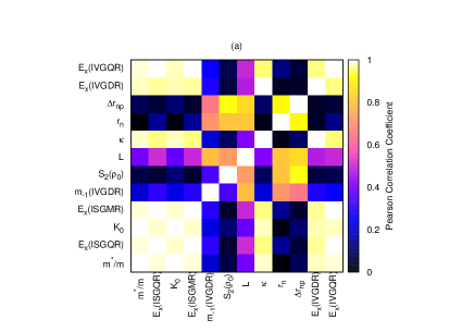
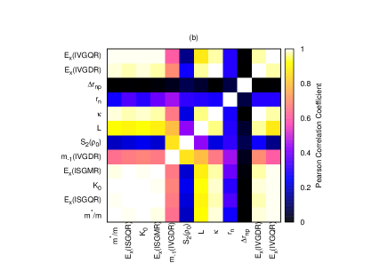
Figure 1: Values of the Pearson-product correlation coefficient calculated among pairs of observables. Panels (a) and (b) corresponds to two different kinds of mimimization procedures, that are discussed in the text.

4.2 Some results from the covariance analysis

Several results obtained via the covariance analysis have been presented in Ref. [25]. Here, we only focus on some illustrative findings that are of relevance in connection with our previous discussion on symmetry energy and other isovector observable.

We have fitted a functional called SLy5-min, that has been built so that to be as close as possible to the original SLy5 force [28, 29]. Details and differences are highlighted in Ref. [25]. We now illustrate what happens to correlations between observables when one varies the fitting protocol.

The original SLy5 functional, and the present Sly5-min functional as well, has been fitted by including in the $\chi^{2}$ as pseudo-data a set of values for the neutron matter equation of state derived by some ab-initio calculation with realistic forces [30]. In the variant that we label as SLy5-a, we have changed in the $\chi^{2}$ the weight associated with these pseudo-data, that is, with the equation of state of neutron matter. In particular, We have increased the value of the error on these points, $\Delta\frac{E}{A}(\rho,\delta=1)$, from $0.1\times\frac{E}{A}(\rho,\delta=1)$ – that corresponds to a 10% relative error – to $0.5\times\frac{E}{A}(\rho,\delta=1)$. The Pearson-product correlation coefficients of this fit are shown in panel (a) of Fig. 1. One can notice a strong correlation between the isovector observables, that are, the neutron radius of ²⁰⁸Pb, $S(\rho_{0})$, $L$ and $m_{-1}$(IVGQR). This result clearly indicates that when a constraint on a property $A$ is relaxed, correlations with other related observables $B$ not included in the fitting protocol become larger.

The second variant we have built is denoted as SLy5-b. In this case, we have kept all terms in the $\chi^{2}$ as in SLy5-min except the equation of state of neutron matter that now is not included at all, and we added instead a very tight constraint on the neutron skin thickness of ²⁰⁸Pb: we have chosen $\Delta r_{np}=0.160\pm 0.001$ fm. Then, panel (b) of Fig. 1 shows another interesting outcome: $\Delta r_{np}$ displays an almost vanishing correlation with all the other quantities. This indicates that when a property $A$ is tightly constrained in the fitting protocol, correlations with other observables $B$ become very small.

5 Conclusions

The most important outcomes of our recent works on the constraints on the density dependence of the symmetry energy imposed by the properties of isovector excitations are

• if one looks at correlations between observables and values or derivatives of the symmetry energy, calculated using a large set of different EDFs, consistent values of $L$ and of the neutron skin thickness in ²⁰⁸Pb are extracted from the study of the IVGDR, IVGQR, PDR and total dipole polarizability [cf., in particular, Eqs. (8), (10), (14) as well as Eqs. (9), (11)];

• some of these correlations are suggested by macroscopic models and, in general, we believe that it would be desirable that correlations emerge from a sound physical picture rather than simply from a numerical analysis;

• models may, or may not, display the correlations that one expects on physical grounds because of the strong impact of the fitting protocols. We have shown that correlations of an observable $A$ with related observables $B$ may emerge (vanish) if the constraint put on $A$ in the fitting protocol is negligible (very tight).

References

- [1] Topical Issue on Nuclear Symmetry Energy, B.A. Li, A. Ramos, G. Verde and I. Vidaña Eds., Eur. Phys. J. A50 (2014).
- [2] M. Bender, P.-H. Heenen, P.-G. Reinhard, Rev. Mod. Phys. 75, 121 (2003).
- [3] I. Vidaña, C. Providência, A. Polls, and A. Rios, Phys. Rev. C80, 045806 (2009).
- [4] L. Trippa, G. Colò, and E. Vigezzi, Phys. Rev. C77, 061304(R) (2008).
- [5] G. Colò, L. Cao, N. Van Giai, L. Capelli, Comp. Phys. Comm. 184, 142 (2013).
- [6] E. Lipparini, S. Stringari, Phys. Rep. 103, 1975 (1989).
- [7] M. Centelles, X. Roca-Maza, X. Viñas, and M. Warda, Phys. Rev. Lett. 102, 122502 (2009).
- [8] S.S. Henshaw, M.W. Ahmed, G. Feldman, A.M. Nathan, H.R. Weller, Phys. Rev. Lett. 107, 22501 (2011).
- [9] X. Roca-Maza, M. Brenna, B.K. Agrawal, P.F. Bortignon, G. Colò, L. Cao, N. Paar, and D. Vretenar, Phys. Rev. C87, 034301 (2013).
- [10] X. Roca-Maza, G. Colò, and H. Sagawa, Phys. Rev. C86, 031306(R) (2012).
- [11] G.A. Lalazissis, T. Nikšić, D. Vretenar and P. Ring, Phys. Rev. C71, 024312 (2005).
- [12] B. A. Brown, Phys. Rev. Lett. 85, 5296 (2000); S. Typel and B. A. Brown, Phys. Rev. C64, 027302(R) (2001).
- [13] N. Paar, D. Vretenar, E. Khan, G. Colò, Rep. Progr. Phys. 70, 691 (2007).
- [14] D. Savran, T. Aumann, A. Zilges, Prog. Part. Nucl. Phys. 70, 210 (2013).
- [15] A. Carbone, G. Colò, A. Bracco, L. Cao, P.F. Bortignon, F. Camera, and O. Wieland, Phys. Rev. C81, 041301(R) (2010).
- [16] Y. Suzuki, K. Ikeda, H. Sato, Prog. Theor. Phys. 83, 180 (1980).
- [17] W. Nazarewicz and P.-G. Reinhard, Phys. Rev. C81, 051303(R) (2010).
- [18] X. Roca-Maza, G. Pozzi, M. Brenna, K. Mizuyama, and G. Colò, Phys. Rev. C85, 024601 (2012).
- [19] D. Vretenar, Y.F. Niu, N. Paar, and J. Meng, Phys. Rev. C85, 044317 (2012).
- [20] D. Vretenar, N. Paar, P. Ring, and T. Nikšić, Phys. Rev. C65, 021301(R) (2001).
- [21] A. Repko, P.-G. Reinhard, V.O. Nesterenko, and J. Kvasil, Phys. Rev. C87, 024305 (2013).
- [22] J. Piekarewicz, B.K. Agrawal, G. Colò, W. Nazarewicz, N. Paar, P.-G. Reinhard, X. Roca-Maza, and D. Vretenar, Phys. Rev. C85, 041302 (2012).
- [23] X. Roca-Maza, M. Brenna, G. Colò, M. Centelles, X. Viñas, B.K. Agrawal, N. Paar, D. Vretenar, J. Piekarewicz, Phys. Rev. C88, 024316 (2013).
- [24] M. Centelles, X. Roca-Maza, X. Viñas, and M. Warda, Phys. Rev. Lett. C82, 054314 (2010).
- [25] X. Roca-Maza, N. Paar, and G. Colò, J. Phys. G (in press) [arXiv:1406.1885].
- [26] P.R. Bevington and D.K. Robinson, Data reduction and error analysis for the physical sciences (McGraw-Hill, New York, 1992).
- [27] J. Dobaczewski, W. Nazarewicz, P.-G. Reinhar, J. Phys. G: Nucl. Part. Phys. 41, 074001 (2014).
- [28] E. Chabanat, P. Bonche, P. Haensel, J. Meyer and R. Schaeffer, Nucl. Phys. A627, 710 (1997).
- [29] E. Chabanat, P. Bonche, P. Haensel, J. Meyer and R. Schaeffer, Nucl. Phys. A635, 231 (1998).
- [30] R.B. Wiringa, V. Fiks, and A. Fabrocini, Phys. Rev. C38, 1010 (1988).