Supermassive Black Holes with High Accretion Rates in Active Galactic Nuclei.
IV. H$\beta$ Time Lags and Implications for Super-Eddington Accretion

Abstract

We have completed two years of photometric and spectroscopic monitoring of a large number of active galactic nuclei (AGNs) with very high accretion rates. In this paper, we report on the result of the second phase of the campaign, during 2013–2014, and the measurements of five new H$\beta$ time lags out of eight monitored AGNs. All five objects were identified as super-Eddington accreting massive black holes (SEAMBHs). The highest measured accretion rates for the objects in this campaign are $\dot{\mathscr{M}}\gtrsim 200$, where $\dot{\mathscr{M}}=\dot{M}_{\bullet}/L_{\rm Edd}c^{-2}$, $\dot{M}_{\bullet}$ is the mass accretion rates, $L_{\rm Edd}$ is the Eddington luminosity and $c$ is the speed of light. We find that the H$\beta$ time lags in SEAMBHs are significantly shorter than those measured in sub-Eddington AGNs, and the deviations increase with increasing accretion rates. Thus, the relationship between broad-line region size ($R_{{}_{\rm H\beta}}$) and optical luminosity at 5100Å, $R_{{}_{\rm H\beta}}-L_{5100}$, requires accretion rate as an additional parameter. We propose that much of the effect may be due to the strong anisotropy of the emitted slim-disk radiation. Scaling $R_{{}_{\rm H\beta}}$ by the gravitational radius of the black hole, we define a new radius-mass parameter ($Y$) and show that it saturates at a critical accretion rate of $\dot{\mathscr{M}}_{c}=6\sim 30$, indicating a transition from thin to slim accretion disk and a saturated luminosity of the slim disks. The parameter $Y$ is a very useful probe for understanding the various types of accretion onto massive black holes. We briefly comment on implications to the general population of super-Eddington AGNs in the universe and applications to cosmology.

1 Introduction

Reverberation mapping (RM) experiments, which measure the delayed response of the broad emission line gas to the ionizing continuum in active galactic nuclei (AGNs), are the best way to map the gas distribution and derive several fundamental properties such as its emissivity-weighted radius and the black hole (BH) mass. The method was suggested by Bahcall et al. (1972) and its theoretical foundation explained in detailed in Blandford & McKee (1982). Numerous RM experiments, since the late 1980s (e.g., Clavel et al. 1991; Peterson et al. 1991, 1993; Maoz et al. 1991; Wanders et al. 1993; Dietrich et al. 1993; Kaspi et al. 2000; Denney et al. 2010; Bentz et al. 2009; Grier et al. 2012; Du et al. 2014; Wang et al. 2014a; Barth et al. 2015), have succeeded in mapping the emissivity distribution of H$\beta$ and several other lines in the broad-line region (BLR) in more than 40 AGNs. BH virial mass measurements based on the method was shown to be consistent with the $M_{\bullet}-\sigma_{*}$ relationship, or with measurements based on stellar dynamics in local objects, where $\sigma_{*}$ is the stellar velocity dispersion in the host galaxy (Ferrarese et al. 2001; Onken et al. 2004; see Kormendy & Ho 2013 for an extensive review). This method is an efficient and routine way to estimate BH mass at basically all redshift, at distances that are well beyond the resolving power of all ground-based telescopes. The RM experiments have been extensively discussed and reviewed in the literature (e.g., Peterson 1993; Kaspi et al. 2000 for earlier works and Shen et al. 2015 and De Rosa et al. 2015 for more recent results).

Most RM experiments, so far, have focused on the time lag of the broad H$\beta$ line ($\tau_{{}_{\rm H\beta}}$ in the rest frame) relative to the AGN continuum luminosity ($\lambda L_{\lambda}$) at rest-frame wavelength of 5100Å (hereafter $L_{5100}$). Results for 41 such measurements, based on AGN luminosity that is corrected for host galaxy contamination, are summarized in Bentz et al. (2013). They lead to a simple, highly significant correlation of the form,

$$R_{{}_{\rm H\beta}}\approx\alpha~{}l_{44}^{\beta}~{}{\rm ltd}\,\,,$$ (1)

where $R_{{}_{\rm H\beta}}=c\tau_{{}_{\rm H\beta}}$ is the emissivity-weighted radius of the BLR and $l_{44}=L_{5100}/10^{44}\rm erg~{}s^{-1}$. We refer to this type of relationship as the $R_{{}_{\rm H\beta}}-L_{5100}$ relationship. The constants $\alpha$ and $\beta$ differ slightly from one study to the next, depending on the number of sources and their exact luminosity range. For the Bentz et al. (2013) work, $\alpha=33.65$ and $\beta=0.533$. Scaling relationships based on other emission lines have been used to estimate BH mass in high-redshift AGNs. These are either based on the Mg ii$\lambda 2798$ line, which is scaled to the H$\beta$ line (e.g., McLure & Dunlop 2004; Vestergaard & Peterson 2006; Shen et al. 2011; Trakhtenbrot & Netzer 2012) or the C iv$\lambda 1549$ line, for which few direct lag measurements are available (e.g., Kaspi et al. 2007). So far, there is not enough information about the dependence of the $R_{{}_{\rm H\beta}}-L_{5100}$ relationship on accretion rate or Eddington ratio $L_{\rm Bol}/L_{\rm Edd}$, where $L_{\rm Bol}$ is the bolometric luminosity, $L_{\rm Edd}=1.5\times 10^{38}(M_{\bullet}/M_{\odot})\rm erg~{}s^{-1}$ is the Eddington luminosity for a solar composition gas, and $M_{\bullet}$ the BH mass.

We are conducting a large RM monitoring campaign targeting high-accretion rate AGNs. The aims are to understand better the physical mechanism powering these sources, the dependence of the $R_{{}_{\rm H\beta}}-L_{5100}$ relationship on accretion rate, and the possibility to use such objects to infer cosmological distances especially at high $z$ (Wang et al. 2013). We coin these sources “super-Eddington accreting massive black holes” (SEAMBHs). Earlier attempts in this direction, based on monitoring narrow-line Seyfert 1 galaxies (NLS1s), failed mostly because of the small variability amplitude of the selected sources (Giannuzzo & Stirpe 1996; Giannuzzo et al. 1998; Shemmer & Netzer 2000; Klimek et al. 2004). Bentz et al. (2010) summarized results for a few NLS1s, and found relatively small $L_{\rm Bol}/L_{\rm Edd}$ for this class of objects and time lags that are not significantly different from the ones given by Equation (1). Our monitoring campaign started in 2012 and its first two phases are already completed. The $\sim 20$ targets observed so far are listed in Table 1. Results from the first phase have been published in Du et al. (2014; hereafter Paper I) and Wang et al. (2014a; hereafter Paper II). We also studied the time-dependent variability of the strong Fe ii  lines in nine of the sources, and the results are reported in Hu et al. (2015, hereafter Paper III). We characterize SEAMBHs by their dimensionless accretion rate, $\dot{\mathscr{M}}=\dot{M}_{\bullet}/L_{\rm Edd}c^{-2}$, where $\dot{M}_{\bullet}$ is the accretion rate. Typical values of this parameter range from a few to $\sim 100$ for the objects in the first phase of the project. Such high accretion rates are characteristics of slim accretion disks (Abramowicz et al. 1988) that are thought to power these objects (Szuszkiewicz et al. 1996; Wang & Zhou 1999; Wang et al. 1999; Mineshige et al. 2000). Paper II shows that such objects may eventually become new standard candles for cosmology.

This paper reports the results of the second year of our RM campaign. Target selection, observation details and data reduction are described in §2. H$\beta$ lags, BH mass and accretion rates are provided in §3. The new H$\beta$ lags are discussed in §4, showing that for a given luminosity, the H$\beta$ lag gets shorter with increasing $\dot{\mathscr{M}}$. In §5 we briefly discuss the implications of the new findings to the understanding of BLR physics and geometry, and to accretion physics. §6 gives a brief summary of the paper. Throughout this work we assume a standard cosmology with $H_{0}=67~{}{\rm km~{}s^{-1}~{}Mpc^{-1}}$, $\Omega_{\Lambda}=0.68$ and $\Omega_{\rm M}=0.32$ (Ade et al. 2014).

2 Observations and data reduction

2.1 Target Selection

Unlike the first phase described in Papers I and II, in which most objects are NLS1s, for the second phase we selected targets from the quasar sample of the Sloan Digital Sky Survey Data Release 7 (SDSS DR7) using the pipeline employed in Hu et al. (2008a). The objects have similar spectroscopic characteristics to the NLS1s from Papers I and II, in particular: 1) strong optical Fe ii lines, 2) narrow ($\lesssim 2000\rm km~{}s^{-1}$) H$\beta$ lines, 3) weak [O iii] lines (Osterbrock & Pogge 1987; Boroson & Green 1992). The objects selected for the first year study are NLS1s with extremely steep $2-10$ keV continuum. For the second year sample reported here, we do not have X-ray data and use, instead, the dimensionless accretion rate $\dot{\mathscr{M}}$, which can be estimated through the physics of thin accretion disks as formulated by Shakura & Sunyaev (1973, hereafter SS73). In such systems, the accretion rate can be directly calculated from the part of the spectrum where $L_{\nu}\propto\nu^{1/3}$, regardless of the value of the BH spin (e.g., Collin et al. 2002; Davis & Laor 2011 and references therein). The only significant uncertainty in this estimate is the disk inclination to the line of sight, $i$ (see more details in Paper II). We take $\cos i=0.75$ in this series of papers. The standard thin disk equations give (see Paper II),

$$\dot{\mathscr{M}}=20.1\left(\frac{l_{44}}{\cos i}\right)^{3/2}m_{7}^{-2},$$ (2)

where $m_{7}=M_{\bullet}/10^{7}M_{\odot}$. For thin accretion disks, we have $L_{\rm Bol}/L_{\rm Edd}=\eta\dot{\mathscr{M}}$, where $L_{\rm Bol}$ is the disk bolometric luminosity, and $\eta$ is the mass-to-radiation conversion efficiency which depends on the BH spin.

When comparing thin to slim accretion disks it is important to note that in both systems, the observed 5100Å emission comes from large disk radii and thus is less influenced by the radial motion of the accretion flow compared with the regions closer in that emit the shorter wavelength photons. At these large radii, Keplerian rotation dominates, radiation cooling locally balances the release of gravitational energy through viscosity, and all effects arising from radial advection and the black hole spin can be neglected. As direct integration of the disk SED is not practical in almost all cases, due to the lack of far-UV observations, measuring $L_{\rm Bol}/L_{\rm Edd}$ directly is not possible, and Equation (2) is the best way to estimate $\dot{\mathscr{M}}$, which is directly related to the SS73 accretion disk model.

To estimate the BH mass, we followed the standard approach and assume that the BLR gas is moving in Keplerian orbits and the rest frame time lags ($\tau_{{}_{\rm H\beta}}$) provide reliable estimates of $R_{{}_{\rm H\beta}}$. This gives,

$$M_{\bullet}=f_{{}_{\rm BLR}}\frac{R_{{}_{\rm H\beta}}V_{\rm FWHM}^{2}}{G}=1.95\times 10^{6}~{}f_{{}_{\rm BLR}}V_{3}^{2}\tau_{10}~{}M_{\odot},$$ (3)

where $G$ is the gravitational constant, $V_{3}=V_{\rm FWHM}/10^{3}\rm km~{}s^{-1}$ is the full-width-half-maximum (FWHM) of the H$\beta$ line profile in units of $10^{3}\rm km~{}s^{-1}$ and $\tau_{10}=\tau_{{}_{\rm H\beta}}/10$days. The factor $f_{{}_{\rm BLR}}$ is calibrated from the known $M_{\bullet}-\sigma$ relation (e.g., Onken et al. 2004; Ho & Kim 2014). This is still a matter of some debate and the quoted uncertainties are large. The study of Ho & Kim (2014) shows that for AGNs in host galaxies with pseudo-bulges, $f_{{}_{\rm BLR}}$ is smaller than in AGNs hosted by classical bulges or ellipticals. However, $f_{{}_{\rm BLR}}$ gets larger for AGNs with higher Eddington ratios. It is not very clear what is the end result of these two opposite trends. For most SEAMBHs in Papers I and II, the host galaxies were observed by the Hubble Space Telescope (HST) and show indications for pseudo-bulges. They also have very high $L_{\rm Bol}/L_{\rm Edd}$. For the present sample we do not have HST images but these sources also are of high $L_{\rm Bol}/L_{\rm Edd}$. Given all this, we use $f_{{}_{\rm BLR}}=1$, as in Papers I and II, but note the large uncertainty on this number.

Employing Equations (1) and (3), we estimated $\dot{\mathscr{M}}$ from Equation (2) for quasars in the SDSS DR7 and selected sources with the highest $\dot{\mathscr{M}}$. We discarded radio-loud objects based on the reported FIRST observations. We also chose a redshift range of $z=0.1-0.3$ and $L_{5100}\lesssim 10^{44.5}\rm erg~{}s^{-1}$ to make sure that the lag, as estimated from Equation (1), can be measured in $5-6$ months of monitoring campaign and magnitude $r^{\prime}\leq 18.0$ to ensure high enough signal-to-noise (S/N). Details of the sources are given in Table 1.

2.2 Photometry and Spectroscopy

The second year observations described here are essentially identical to those of the first year, and readers are referred to Papers I and II for detailed information about the telescope and spectrograph. In short, the telescope is a 2.4 m alt-azimuth mounted Ritchey-Chrétien located in Lijiang, Yunnan Province, and operated by the Yunnan Observatories. We use the Yunnan Faint Object Spectrograph and Camera (YFOSC) with a back-illuminated 2048$\times$4608 pixel CCD covering a field of $10^{\prime}\times 10^{\prime}$. The differences between the first and 2nd year observations are: 1) we adopted a $5^{\prime\prime}$-wide slit, compared with the previously used $2.5^{\prime\prime}$ slit, to minimize the influence of atmospheric differential refraction, and used Grism 3 with spectral resolution of 2.9Å/pixel and wavelength coverage of 3800-9000Å. 2) Instead of the Johnson $V$ filter used in 2012, we used SDSS $r^{\prime}$-band filter to avoid the potential contamination by emission lines such as H$\beta$ and H$\alpha$. 3) The observations now include photometry from the Wise Observatory, 1m telescope in Israel, where we used a Princeton Instruments CCD camera, an SDSS $r^{\prime}-$band filter and a typical exposure time of 900 sec. The reduction of the Wise and Yunnan Observatory photometry data was done in a standard way using IRAF routines. For the Lijiang data, the reduction, and the procedures to measure 5100Å and F(H$\beta$), are given in Papers I while for Wise data, the flux measurements were done using point-spread function photometry. The light curves were produced by comparing the instrumental magnitudes to those of constant stars in the field (see, e.g., Netzer et al. 1996, for details). The uncertainties on the photometric measurements include the fluctuations due to photon statistics and the scatter in the measurement of the stars used. Detailed information of observations, such as, comparison stars etc. is provided in Table 1. We also list the critical S/N used as a low threshold to reject poor weather condition observations.

The 5100Å light curves used in the analysis were obtained by inter-calibration of the 5100Å spectroscopy, $r^{\prime}-$band Lijiang 2.4-m photometry, and $r^{\prime}-$band Wise Observatory photometry. We used the Bayesian algorithm described in Li et al. (2014), who assume that the AGN optical continuum variations follow a damped random walk model (Kelly et al. 2009; Li et al. 2013). We applied a multiplicative scale factor and an additive flux adjustment to bring the different measurements to a common flux scale. The algorithm performs inter-calibration on all the datasets simultaneously. This enables us to relax the requirements for the sampling rates and retain the highest achievable temporal resolution. We selected the Lijiang spectroscopy as the common scale. The best parameters for the inter calibration are determined by a Markov chain Monte Carlo (MCMC) implementation. In that way we get the inter-calibrated continuum light curves of photometry (Lijiang and Wise data) and spectral continuum (Lijiang data). Finally, the combined light curves are obtained by averaging all the points of a same day in the inter-calibrated light curves. All the continuum and H$\beta$ light curves for the eight objects are listed in Tables $2-5$, and shown in Figure 1. We also calculated the mean and RMS (root mean square) spectra and present them in Appendix A where we briefly discuss these data.

2.3 Host Galaxies

Most of the objects described in Papers I and II had previous HST images that were used to subtract the host galaxy contribution at 5100Å. Such information is not available for the sources reported in this paper. Instead, we used the empirical relation suggested by Shen et al. (2011) based on SDSS spectra: $L_{5100}^{\rm host}/L_{5100}^{\rm AGN}=0.8052-1.5502x+0.912x^{2}-0.1577x^{3}$, for $x<1.053$, where $x=\log\left(L_{5100}^{\rm tot}/10^{44}{\rm erg~{}s^{-1}}\right)$ and $L_{5100}^{\rm tot}$ is the total emissions of AGNs and their host at 5100Å. For $x>1.053$ we have $L_{5100}^{\rm host}\ll L_{5100}^{\rm AGN}$, and the host contamination can be neglected. These authors obtained the geometric mean composite spectra for objects binned in $\log L_{5100}$ normalized at 3000Å  and found spectral flattening toward long wavelengths. The flatten part of the spectra depends on host contaminations. This empirical relation was obtained by the difference of the flatten part through comparisons among the spectra for quasars in 5100Å  luminosity bins.

The above procedure was developed for the $3^{\prime\prime}$ SDSS fiber noted as $x_{{}_{3^{\prime\prime}}}$. This is considerably smaller than the effective aperture ($5^{\prime\prime}$) used by us. Denote $x_{{}_{5^{\prime\prime}}}$ as the flux measured from our mean spectra and $\Delta x=|x_{{}_{3^{\prime\prime}}}-x_{{}_{5^{\prime\prime}}}|$. We find that on average $\Delta x/x_{{}_{3^{\prime\prime}}}<0.3$. We also find that the differences in $L_{5100}^{\rm host}/L_{5100}^{\rm AGN}$ between the $3^{\prime\prime}$ fiber and our $5^{\prime\prime}$ aperture is less than 10%. The fraction is estimated by comparing $F_{5^{\prime\prime}}$ and $F_{3^{\prime\prime}}$ fluxes at 5100Å  in our sample, where $F_{5^{\prime\prime}}$ and $F_{3^{\prime\prime}}$ are measured from Lijiang and SDSS observations, respectively. In general, more than 90% of the light is contained within the $3^{\prime\prime}$ fiber for $z\sim 0.2$ quasars. Thus, the present subtraction of host contamination is quite robust, and the added uncertainty due to this difference is not larger than the intrinsic uncertainty in Shen et al.’s expression.

3 H$\beta$ Lags, Black Hole Mass and Accretion Rates

We used a standard cross-correlation analysis to determine the lags of the H$\beta$ line relative to the combined 5100Å continuum. The procedure is quite standard and was described, in detail, in Papers I and II, where we also list all the relevant references. The uncertainties on the lags are determined through the “flux randomization/random subset sampling” method (RS/RSS) (Peterson et al. 1998, 2004), the cross-correlation centroid distribution (CCCD) and cross-correlation peak distribution (CCPD) generated by RS/RSS method (Maoz & Netzer 1989; Peterson et al. 1998, 2004; Denney et al. 2006, 2010 and reference therein), which are shown in Figure 1. For a successful detection of H$\beta$ lag we require: 1) non-zero lag from the CCF peak and 2) a maximum correlation coefficient larger than 0.5.

Five of the eight sources show well-determined lags. All these sources are listed in Table 6. The other three failed our above criteria. Figure 1 shows that the CCFs of two of them (J094422 and J100055) show two comparable peaks and no significant H$\beta$ lags. The third source, J080131, has an unusual combination of line and continuum light curves. The continuum light curve shows a well-determined, broad feature followed by two major short ”bursts” centered at around JD24566000+, $120$ and $140$. The H$\beta$ light curve shows a clear response to the first continuum dip and burst feature, but no response to the two shorter duration features. The CCF of the entire campaign has a low peak, at $r_{\rm max}\simeq 0.5$, which is consistent with a zero lag. Carrying the analysis for the first 70 days only, as shown in the second diagram of J080131 panel in Figure 1, we found a very significant peak with a centroid lag of $11.5_{-3.6}^{+8.4}$ days (with a very high coefficient of $r_{\rm max}=0.81$) in rest-frame.

Our search of the literature shows that the unusual combination of line and continuum light curves observed in J080131 is rare [see similar, but not identical, behavior in NGC 7469 (Peterson et al. 2014) and in the UV light curve of NGC 5548 (De Rosa et al. 2015)]. We can think of various scenarios that could cause such an event in a SEAMBH with extremely high accretion rate. For example, the inner part of slim disks can be so thick that self-shadowing effects lead to strong anisotropy of the emitted radiation. The signal received and measured by a remote observer can differ substantially from the ionizing radiation that reaches the H$\beta$-emitting clouds (see discussions by Wang et al. 2014b). Given the rarity of such objects, we have no way to test this idea and thus do not include this object in the remaining analysis.

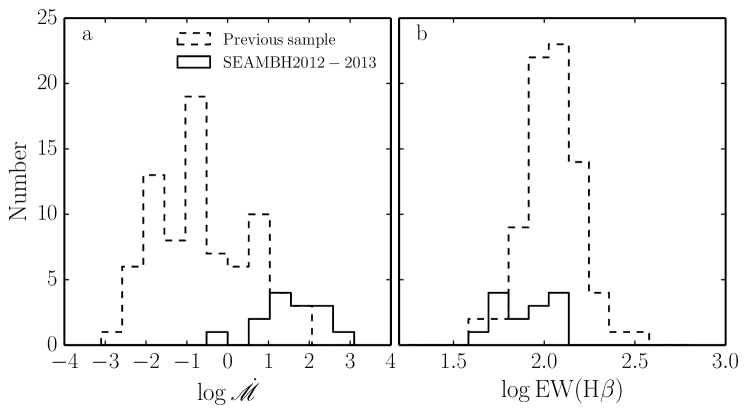
Figure 2: The distribution of dimensionless accretion rates of the mapped AGNs and quasars. The previous sample refers to the sample of all mapped AGNs summarized by Bentz et al. (2013) (the repeated monitored AGNs are regarded as individual ones), and adds four recently mapped AGNs: NGC 7469 updated by Peterson et al. (2014), KA 1858+4850 (Pei et al. 2014), Mrk 1511 (Barth et al. 2013) and NGC 5273 (Bentz et al. 2014). The dashed line is for the previous sample and the solid is for the SEAMBH sample. Our campaign selected those candidate sources with extremely high accretion rates ($\dot{\mathscr{M}}\gtrsim 10$). Though some sources monitored previously have $\dot{\mathscr{M}}\sim 10$, most of them have lower accretion rates. Right panel shows the distribution of EW(H$\beta$), showing that SEAMBH sample tends to have low EW(H$\beta$).

We used Equations 2 and 3 to calculate accretion rates, $\dot{\mathscr{M}}$ and BH masses for the five sources listed in Table 6. The details of the procedure are given in papers I and II and the distributions of $\dot{\mathscr{M}}$ in the two groups of the previously and currently monitored objects are shown in Figure 2. As clearly shown in the diagram, our Lijiang-observed sources occupy the high tail of the $\dot{\mathscr{M}}$ distribution. This is not surprising given the way we selected our targets. We also show in Figure 2 the equivalent width (EW) distribution of H$\beta$. On average, our high accretion rate sources have lower mean EW(H$\beta$). An anti-correlation between EW(H$\beta$) and $L_{\rm Bol}/L_{\rm Edd}$ has been found in other samples with less accurate rates, in which BH mass is estimated by the $R_{{}_{\rm H\beta}}-L_{5100}$ relation (e.g., Netzer et al. 2004).

In Paper II we classified SEAMBHs as those objects with $\dot{m}=\eta\dot{\mathscr{M}}\geq 0.1$. This is based on the idea that beyond this value, the accretion disk becomes slim and the radiation efficiency is reduced due to photon trapping and other effects. Since we cannot observe the entire SED, we have no direct way to measure $L_{\rm Bol}/L_{\rm Edd}$, and this criterion is used as an approximate tool for identifying SEAMBH candidates. To be on the conservative side, we chose the lowest possible efficiency, $\eta=0.038$ (retrograde disk with $a=-1$, see Bardeen et al. 1972). Thus SEAMBHs are objects with $\dot{\mathscr{M}}=2.63$. For simplicity, in this paper we use $\dot{\mathscr{M}}_{\rm min}=3$ as the required minimum. Later on, in §5, we introduce an empirical way, based on our own mass measurements, to define this group more accurately.

Table 6 lists all observables, $M_{\bullet}$ and $\dot{\mathscr{M}}$ for the first (SEAMBH2012) and second (SEAMBH2013) year observations. All objects, except for MCG $+06-26-012$ (see note in the table caption), show $\dot{\mathscr{M}}>3$, indicating they are SEAMBHs. In Paper III, more accurate measurements of H$\beta$ lags have been derived by using a scheme of simultaneously fitting spectra of host and AGNs. The newly measured lags are the ones listed table 6. Comparing with the previous measurements in Papers I and II, the updated lags are consistent with the previous ones, but the error bars are much smaller. Including our new observations, the majority of SEAMBHs with RM-based mass measurements come from our Lijiang RM campaign.

4 H$\beta$ Time Lags in SEAMBHs

To understand better the fundamental differences between high and low $\dot{\mathscr{M}}$ sources, we must use the measured correlation between time lag and source luminosity for all RM AGNs. For this, we have to take into account that some of the sources have been mapped more than once and hence there are various measured values for their luminosity, time lag, and FWHM(H$\beta$), for the same BH mass. There are two possible ways to address this issue. The first is to average the BH mass from the individual campaigns, and then obtain mean (or median) values for $L_{5100}$, $L_{{}_{\rm H\beta}}$ and the time lag. This scheme, which was used in Kaspi et al (2005), Bentz et al (2009) and other papers, is referred here as the “average scheme”. The second is to treat the independent RM campaigns of a single object as different objects (e.g., Bentz et al. 2013). We call this the “direct scheme”.

The goal of the present paper is to find the basic properties of the central power house, presumably an accretion disk, as a function of BH mass and normalized accretion rate. The measured H$\beta$ time lag is the tool we use to study these properties. This is changing with the ionizing continuum but it does not represent real changes in the gas distribution in the BLR during one observing season. Since the BH mass does not change on a short time scale, and the time scale to change the global accretion rate through the disk is also very long, we must be seeing short time scale fluctuations that do not change these fundamental properties but, nevertheless, affect the ionization of the BLR. To understand the population properties, we must give equal weights to all objects, i.e., use the average scheme approach. This means that the mean luminosity is used to derive $\dot{\mathscr{M}}$. This can be done during one campaign that lasts a few months, or during several campaigns that last a few years. The only exception is, perhaps, when the total time exceeds the dynamical time scale of the BLR.

The direct scheme can be useful to derive other properties, such as the ionization distribution across a “typical BLR”. While this is not the goal of the present work, we have calculated all the fundamental correlations discussed below using this approach, too, and show them in Appendix B. We note that despite the fundamentally different approaches, which result in a different BH mass distribution (since several masses are counted more than once), the results are not very different.

4.1 Continuum luminosity $vs.$ BLR Size

Table 7 lists the objects summarized by Bentz et al. (2013), plus a few newly mapped sources. Since some of the procedures used in earlier campaigns differ in several aspects, we decided to apply the same uniform procedure for all the sources. For objects with multiple RM measurements, our procedure for obtaining the average values is as follows: We first calculate $M_{\bullet}$ for each of the individual campaigns and then average all these values, using weighted standard deviations, to get a mean $M_{\bullet}$ and its error. This value is used to obtain individual values of $\dot{\mathscr{M}}$ for the various campaigns, using $L_{5100}$ from this campaign. The mean $\dot{\mathscr{M}}$ for the object is the average of the individual $\dot{\mathscr{M}}$, and its errors include the standard deviation. For the mean luminosity and $\tau_{{}_{\rm H\beta}}$, we used logarithmic averages.

Regarding BH mass calculations in individual campaigns, this is more problematic since some works used the RMS spectrum (e.g., Peterson et al. 2004; Bentz et al. 2009b; Denney et al. 2010; Grier et al. 2012) while others prefer the use of FWHM(H$\beta$) (e.g., Kaspi et al. 2005). Our procedure is based on the FWHM method (see explanation in Papers I and II). As shown recently in Woo et al. (2015), the scatter in the scaling parameter ($f_{\rm BLR}$) derived in this method is very similar to the scatter in the method based on the RMS spectrum.

We have therefore collected from the literature all the required information about the H$\beta$ line and carried out our own mass measurements for the sources where earlier mass measurements were based on the RMS method. In most of the cases, the agreement between the older RMS method and the value obtained here is within the uncertainty on the BH mass. In a few cases (five objects: NGC 4051, NGC 4151, PG 0804+761, PG 1613+658 and PG 2130+099) the deviation is larger which we interpret as unrealistically small uncertainty on the mass. The deviation is generally smaller than $\sim 0.5$ dex except for NGC 4051 where the deviation is $\sim 0.7$dex. Some more details for FWHM measurements of a few objects are given in the caption of Table 7. We list all the measured values and their averages in this table.

All correlations shown in this paper were calculated with the FITEXY method in the version adopted by Tremaine et al. (2002), where scatter is allowed for by increasing the uncertainties in small steps until $\chi^{2}$ is about unity (this is typical for many of our correlations). We also used the BCES method (Akristas & Bershady 1996) but prefer not to use its results since it is known to give unreliable results in samples containing a few outliers (there are a few objects with quite large uncertainties of $\dot{\mathscr{M}}$).

Figure 3a shows H$\beta$ lags versus $L_{5100}$ for all the observations of mapped AGNs (i.e., multiple measurements for each object when available). Our objects are marked with blue (first year, data reported in Papers I and II) and red (second year, this paper). Using the data in Table 7 we get:

$$(1.45\pm 0.03)+(0.50\pm 0.03)\log l_{44} ({\rm entire~{}sample}),$$ (4a)

$$(1.54\pm 0.03)+(0.53\pm 0.03)\log l_{44} (\dot{\mathscr{M}}<3),$$ (4b)

$$(1.30\pm 0.05)+(0.54\pm 0.06)\log l_{44} (\dot{\mathscr{M}}\geq 3),$$ (4c)

with intrinsic scatters $\sigma_{\rm in}=(0.21,0.15,0.24)$ for (4a, 4b, 4c), respectively. The regression for the $\dot{\mathscr{M}}<3$ sample is almost identical to Bentz et al. (2013). Equations (4b) and (4c) show different intercepts for the $\dot{\mathscr{M}}<3$ and the $\dot{\mathscr{M}}\geq 3$ samples. Most of the SEAMBHs from our campaign are located below the $R_{{}_{\rm H\beta}}-L_{5100}$ relation, increasing the scatter in the relationships. For more extreme SEAMBHs with $\dot{\mathscr{M}}>10$, the regression shows $\log(R_{{}_{\rm H\beta}}/{\rm ltd})=(1.18\pm 0.07)+(0.48\pm 0.10)\log l_{44}$, indicating they deviate from the $\dot{\mathscr{M}}<3$ group more than the $\dot{\mathscr{M}}\geq 3$ group. It is clear that the SEAMBH sources increase the scatter considerably, especially over the limited luminosity range occupied by the new sources.

In the following analysis, we use the averaged lags and the averaged mass as listed in Table 7 (note that unlike in paper-II, here we include in the analysis the few radio-loud AGNs with measured time lags and BH mass). In Figure 3c, we divided the population into two sub-groups, those with $\dot{\mathscr{M}}\geq 3$ (11 from earlier studies and 13 from our study) and those with $\dot{\mathscr{M}}<3$. The diagram emphasizes that much of the intrinsic scatter is caused by a systematic deviation of the large $\dot{\mathscr{M}}$ sources towards shorter lags. The regression calculations give

$$(1.45\pm 0.04)+(0.50\pm 0.03)\log l_{44} ({\rm entire~{}sample}),$$ (5a)

$$(1.55\pm 0.04)+(0.53\pm 0.04)\log l_{44} (\dot{\mathscr{M}}<3),$$ (5b)

$$(1.32\pm 0.06)+(0.53\pm 0.06)\log l_{44} (\dot{\mathscr{M}}\geq 3),$$ (5c)

with intrinsic scatters of $\sigma_{\rm in}=(0.21,0.16,0.22)$ for (5a, 5b, 5c), respectively. The slope of the correlation for the SEAMBH sample, those with $\dot{\mathscr{M}}\geq 3$, is comparable to that of sub-Eddington AGNs, but the normalisation is significantly different. Clearly, the H$\beta$ region of SEAMBHs is smaller than sub-Eddington AGNs (see the different intercepts in Equations 5b and 5c).

A more complete approach is to analyze the dependence of $\tau_{{}_{\rm H\beta}}$ on $L_{5100}$ and $\dot{\mathscr{M}}$ together, however, several reasons prevent us from performing such an analysis. First, the current sample is still small; and second the luminosity range of SEAMBHs is very narrow. There are only 4 luminous SEAMBHs (PG 0026+129, PG 1211+143, PG 1226+023, PG 1700+518) identified from the previous campaigns, but their $\dot{\mathscr{M}}=(4.5,6.9,5.0,12.0)$, respectively, are smaller than the average of this group. Thus, the search for a new relationship of the type of $R_{{}_{\rm H\beta}}=R_{{}_{\rm H\beta}}(L_{5100},\dot{\mathscr{M}})$ will have to wait for future observations of luminous, high accretion rate sources.

4.2 H$\beta$ luminosity $vs.$ BLR Size

Figure 3c shows the new $R_{{}_{\rm H\beta}}-L_{{}_{\rm H\beta}}$ relationship. Such relationships have been used in the past to supplement the continuum-based relationships and to correlate the BLR size more closely with the ionizing continuum radiation (see e.g., Kaspi et al. 2005). The regression analysis gives,

$$(1.30\pm 0.03)+(0.51\pm 0.03)\log L_{\rm H\beta,42} ({\rm entire~{}sample}),$$ (6a)

$$(1.36\pm 0.04)+(0.52\pm 0.04)\log L_{\rm H\beta,42} (\dot{\mathscr{M}}<3),$$ (6b)

$$(1.21\pm 0.06)+(0.53\pm 0.06)\log L_{\rm H\beta,42} (\dot{\mathscr{M}}\geq 3),$$ (6c)

where $L_{\rm H\beta,42}=L_{{}_{\rm H\beta}}/10^{42}~{}{\rm erg~{}s^{-1}}$, and $\sigma_{\rm in}=(0.20,0.18,0.22)$ for (6a,6b,6c), respectively. As in the continuum luminosity case, the inferred BLR size for SEAMBHs is smaller than the size of the sources with $\dot{\mathscr{M}}<3$ but the differences are smaller in this case.

The $R_{{}_{\rm H\beta}}-L_{{}_{\rm H\beta}}$ relationship has been examined by Wu et al. (2004) and Kaspi et al. (2005). A comparison with the results of these papers shows similar intercepts but different slopes, with the present slopes being significantly flatter than $0.685\pm 0.106$ found in Wu et al. (2004) and $0.694\pm 0.064$ found by Kaspi et al. (2005). It is not at all clear that these are significant variations since the present sample is much larger and the distribution of sources along the $L_{{}_{\rm H\beta}}$ axis is quite different. The correlations involving $L_{5100}$ and $L_{{}_{\rm H\beta}}$ (Figure 3 and Figure 9 in Appendix B) show a very similar scatter but, for a given H$\beta$ luminosity, SEAMBHs have shorter lags compared with low-accretion rate AGNs. Such differences may be related to the properties of slim accretion disks (Wang et al. 2014b), or other types of anisotropies (e.g., Netzer 1987; O’Brien et al. 1994; Goad & Wanders 1996; Ferland et al. 2009).

4.3 $\dot{\mathscr{M}}-$dependent BLR Size

To test the dependence of the BLR size on accretion rates, we define a new parameter, $\Delta R_{{}_{\rm H\beta}}=\log\left(R_{{}_{\rm H\beta}}/R_{{}_{{\rm H\beta},R-L}}\right)$ that specifies the deviations of individual objects from the $R_{{}_{\rm H\beta}}-L_{5100}/L_{{}_{\rm H\beta}}$ relationship of the sub-sample of $\dot{\mathscr{M}}<3.0$ sources (i.e., $R_{{}_{{\rm H\beta},R-L}}$ as given by Equations 4b, 5b and 6b). The scatter of $\Delta R_{{}_{\rm H\beta}}$ is calculated by $\sigma=\left[\sum_{i}\left(\Delta R_{{\rm H\beta},i}-\langle\Delta R_{{\rm H\beta}}\rangle\right)^{2}/N\right]^{1/2}$, where $N$ is the number of objects and $\langle\Delta R_{{\rm H\beta}}\rangle$ is the averaged value. Figure 3 provides the value of $\sigma$ for comparison.

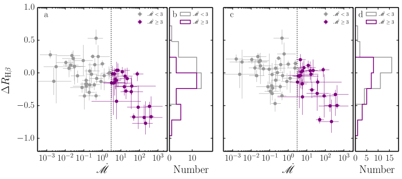
Figure 4: Panels (a, b) and (c, d) show the $\Delta R_{{}_{\rm H\beta}}-\dot{\mathscr{M}}$ relation and $\Delta R_{{}_{\rm H\beta}}$ distributions for $R_{{}_{\rm H\beta}}-L_{5100}$ and $R_{{}_{\rm H\beta}}-L_{{}_{\rm H\beta}}$ relations, respectively. The dotted lines indicate $\dot{\mathscr{M}}=3$ in panel a and c. Both panels show that $\Delta R_{{}_{\rm H\beta}}\sim 0$ up to $\dot{\mathscr{M}}\sim 3$, beyond which $|\Delta R_{{}_{\rm H\beta}}|$ increases with $\dot{\mathscr{M}}$. This implies that, relative to normal AGNs of the same 5100Å  luminosity, SEAMBHs have H$\beta$ lags that become systematically shorter with increasing accretion rate.

Figure 4 shows plots of $\Delta R_{{}_{\rm H\beta}}$ versus $\dot{\mathscr{M}}$, and $\Delta R_{{}_{\rm H\beta}}$ distributions for the $\dot{\mathscr{M}}\geq 3$ and $\dot{\mathscr{M}}<3$ samples. A Kolmogorov-Smirnov (KS) test comparing the two shows that the probability of the same parent distributions is $p_{{}_{\rm KS}}=0.0054$ for the $R_{{}_{\rm H\beta}}-L_{5100}$ case and $p_{{}_{\rm KS}}=0.014$ for $R_{{}_{\rm H\beta}}-L_{{}_{\rm H\beta}}$ case. This provides a strong indication that the main cause of deviation from the old $R_{{}_{\rm H\beta}}-L_{5100}$ relationship (or the $R_{{}_{\rm H\beta}}-L_{5100}$ relationship for the sub-Eddington AGNs) is the extreme accretion rate. Thus, a single $R_{{}_{\rm H\beta}}-L_{5100}$ relationship for all AGNs is a poor approximation for a more complex situation where both the luminosity and the accretion rate determine this relationship. From the regression, we get the dependence of the deviations of $R_{{}_{\rm H\beta}}$ from the $R_{{}_{\rm H\beta}}-L_{5100}$ relation in Figure 4a

$$\Delta R_{{}_{\rm H\beta}}=(0.36\pm 0.13)-(0.46\pm 0.10)\log\dot{\mathscr{M}}~{}~{}~{}({\rm for~{}\dot{\mathscr{M}}\geq 3}),$$ (7)

with $\sigma_{\rm in}=0.07$. From the $R_{{}_{\rm H\beta}}-L_{\rm H\beta}$ relation in Figure 4c, we get

$$\Delta R_{{}_{\rm H\beta}}=(0.33\pm 0.15)-(0.38\pm 0.10)\log\dot{\mathscr{M}}~{}~{}~{}({\rm for~{}\dot{\mathscr{M}}\geq 3}),$$ (8)

with $\sigma_{\rm in}=0.13$. We have tested the above correlations also for $\dot{\mathscr{M}}<3$. The FITEXY regressions give slopes of around zero with very large uncertainties, $\Delta R_{{}_{\rm H\beta}}\propto\dot{\mathscr{M}}^{-0.085\pm 0.051}$ and $\Delta R_{{}_{\rm H\beta}}\propto\dot{\mathscr{M}}^{-0.059\pm 0.054}$ for Figure 4a and 4c, respectively, implying that $\Delta R_{{}_{\rm H\beta}}$ does not correlate with $\dot{\mathscr{M}}$ for $\dot{\mathscr{M}}<3$ group. All this confirms that $\dot{\mathscr{M}}$ is an additional parameter controlling the $R_{{}_{\rm H\beta}}-L_{5100}$ relation in AGNs with high accretion rates.

To summarize, the new SEAMBHs observed in 2012 and 2013 significantly increase the scatter of the $R_{{}_{\rm H\beta}}-L_{5100}$ relation. We find that SEAMBHs have significantly shorter lags than those of sub-Eddington AGNs with similar 5100Å  luminosity, and the shortened lags increase with the dimensionless accretion rate. Given this, we recommend to use Equation (4b) or (5b) when trying to estimate the BLR size in sub-Eddington AGNs. We suggest that the dependence of $R_{{}_{\rm H\beta}}$ on the dimensionless accretion rate could be a consequence of the anisotropic radiation of slim disks. We come back to this issue in the following section.

5 Discussions

The new results presented here illustrate that the small scatter in the earlier $R_{{}_{\rm H\beta}}-L_{5100}$ relationships (Kaspi et al. 2005; Bentz et al. 2013 and references therein), only applies to low accretion rate AGNs, which, according to our definition, are sources with $\dot{\mathscr{M}}<3$. The addition of high accretion rate sources, those referred to as SEAMBHs, changes this picture. The scatter increases and there is a clear, statistically significant tendency for AGNs with higher accretion rates to show smaller $R_{{}_{\rm H\beta}}$. Moreover, the deviation increases with $\dot{\mathscr{M}}$. This holds for both $L_{5100}$ and $L_{{}_{\rm H\beta}}$ although the deviations are larger when using the 5100Å luminosity. The deviations are most noticeable over the luminosity range where most SEAMBHs are concentrated, between $10^{43}$ and $few\times 10^{44}\rm erg~{}s^{-1}$. Below we explore the physical implications of the new results focusing on the earlier suggestion (Paper II) that SEAMBHs are powered by slim accretion disks with properties that are considerably different from those of thin disks.

5.1 $\dot{\mathscr{M}}$ and the Origin of the Shorter Time Lag

The deviations from the earlier $R_{{}_{\rm H\beta}}-L_{5100}$ relationship raise several interesting possibilities that can explain the new results. The first possibility is that the ionizing flux reaching the BLR, which determines its RM-measured size, is different from the flux inferred by a remote observer due to an unusual SED and/or the anisotropy of the radiation emitted from the disk. This possibility has been mentioned in the past with regards to the covering factor and the level of ionization of the BLR. Netzer (1987) presented a detailed model where the combination of an angle-dependent SED of geometrically thin accretion disks (see also Czerny & Elvis 1987; Li et al. 2010 for geometrically thick parts of the disks), with an isotropic X-ray source, results in a weaker ionizing continuum along the plane of the disk compared with the pole-on direction. This will result in a complicated angle-dependent level of ionization. The recent work by Wang et al. (2014b) suggests that large SED variations, especially in the ionizing luminosity as a function of the polar angle, will be most noticeable in slim accretion disks where the anisotropy of the disk is more extreme because of self-shadowing effects. Such a geometry would lead to a smaller emissivity-weighted BLR radius at large angles relative to the polar axis. The second possibility is that much of the effect is due to the change of the bolometric luminosity with polar angle due to the reasons discussed above. This will reduce the dust sublimation radius that has a large effect on the measured RM size (see below). Obviously, the covering factor of the BLR, which determines $L_{{}_{\rm H\beta}}$, and the anisotropy of the Balmer line emission, could also affect these relationships.

The search for a direct ionizing luminosity indicator initiated several attempts to replace $L_{5100}$ by $L_{{}_{\rm H\beta}}$ in the $R_{{}_{\rm H\beta}}-L_{5100}$ relationship because H$\beta$ responds more directly to the ionizing luminosity (e.g., Peterson 1993). Kaspi et al. (2005) show that this substitution had no affect on the deduced BLR size. Similar ideas have been proposed by Wang and Zhang (2003), Wu et al. (2004), and others. Our new observations hint to the possibility that the changes in the $L_{{}_{\rm H\beta}}$ relationship relative to the relationship for the $\dot{\mathscr{M}}<3$ group are smaller than in the $L_{5100}$ case. Unfortunately, the relatively small size of the SEAMBH sample prevents us from quantifying these ideas.

5.2 Accretion Disks and the Maximum Size of the BLR

5.2.1 Geometrically thin disks

Here we explore the possibility that the observed changes in BLR as a function of $\dot{\mathscr{M}}$ are due to the transition from thin ($\dot{\mathscr{M}}<3$) to slim ($\dot{\mathscr{M}}\geq 3$) disks. To start, we express the measured H$\beta$ lags in units of the gravitational radius, $R_{\rm g}=1.5\times 10^{5}(M_{\bullet}/M_{\odot})$ cm. Since $R_{{}_{\rm H\beta}}\propto l_{44}^{b}$ (Equation 1), and $l_{44}\propto\dot{\mathscr{M}}^{2/3}M_{\bullet}^{4/3}$ (Equation 2, recast), we expect

$$r_{{}_{\rm H\beta}}=\frac{R_{{}_{\rm H\beta}}}{R_{\rm g}}=1.9\times 10^{4}~{}\dot{\mathscr{M}}^{0.35}m_{7}^{-0.29},$$ (9)

where we use Equation (5b). Equation (9) concisely mergers the empirical $R_{{}_{\rm H\beta}}-L_{5100}$ relation with the basic expectations of geometrically thin disks.

We now defined a new parameter, $Y=m_{7}^{0.29}r_{{}_{\rm H\beta}}$, which we coin “the radius-mass parameter”, i.e.

$$Y=1.9\times 10^{4}\dot{\mathscr{M}}^{0.35}.$$ (10)

We calculated this combined parameter for all sources in order to test whether it depends on accretion rate. This test would provide clues about the various modes of accretion and their relationship with the size of the BLR.

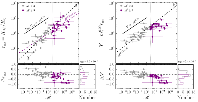
Figure 5: Black hole mass-scaled BLR and the radius-mass parameter versus dimensionless accretion rate. In each panel, there are three plots to show their relation and deviations. Correlations and probabilities of KS tests are marked in the plots. Panel a shows that the $\dot{\mathscr{M}}<3$ sample has a steeper correlation than that given by Equation (9). Panel b shows that SEAMBHs deviate from this relation and that $Y$ is independent of $\dot{\mathscr{M}}$. Clearly $Y$ behaves in a different way in the two accretion rate groups.

Similar to the definition of $\Delta R_{{}_{\rm H\beta}}$ in Section 4.3, we define $\Delta X=\log\left(X/X_{\rm reg}\right)$, where $X$ is the measured value for individual sources and $X_{\rm reg}$ is the value obtained for the group from the regression analysis. In this section we consider two cases, $X=r_{{}_{\rm H\beta}}$ and $X=Y$. The various tests performed on the accretion rate groups are shown in Figure 5 and discussed below.

Our first test for $r_{{}_{\rm H\beta}}$ is performed on the two accretion rate groups, $\dot{\mathscr{M}}<3$ and $\dot{\mathscr{M}}\geq 3$. Figure 5a shows the $r_{{}_{\rm H\beta}}-\dot{\mathscr{M}}$ relation. For $\dot{\mathscr{M}}<3$ objects, we find $r_{{}_{\rm H\beta}}\propto\dot{\mathscr{M}}^{0.50\pm 0.08}$ with $\sigma_{\rm in}=0.24$, which is steeper than expected (Equation 9). By contrast, $r_{{}_{\rm H\beta}}\propto\dot{\mathscr{M}}^{0.35\pm 0.12}$ for the $\dot{\mathscr{M}}\geq 3$ group, consistent with Equation (9). It is clear that the $r_{{}_{\rm H\beta}}-\dot{\mathscr{M}}$ relation is markedly different for the two groups, suggesting that SEAMBHs are physically distinct from sub-Eddington AGNs. $\Delta r_{{}_{\rm H\beta}}$ and its distributions are shown in the lower panels of Figure 5a. A KS test gives the probability of $p_{{}_{\rm KS}}=1.3\times 10^{-3}$ and demonstrates the differences again for the $\dot{\mathscr{M}}\geq 3$ and the $\dot{\mathscr{M}}<3$ groups. We suspect that the deviations from the expected dependences on $\dot{\mathscr{M}}^{0.35}$ are due to the dependence on $m_{7}$ in our sample that contain a large range of BH mass.

Figure 5b shows the $Y-\dot{\mathscr{M}}$ relation, which has much smaller scatter than the $r_{{}_{\rm H\beta}}-\dot{\mathscr{M}}$ relation, for both groups. The regression gives $Y\propto\dot{\mathscr{M}}^{0.41\pm 0.07}$ for the $\dot{\mathscr{M}}<3$ group with $\sigma_{\rm in}=0.15$, which, within the errors, agrees well with Equation (10) confirming the idea of thin accretion disks in objects with $\dot{\mathscr{M}}<3$. The diagram clearly shows a change of slope at a transition accretion rate of $\dot{\mathscr{M}}_{c}\gtrsim 3$ from a rising to an almost horizontal constant (saturated) value. This transition corresponds to a saturated$-Y$ of $Y_{\rm sat}\sim 3\times 10^{4}$. This is consistent with the idea that beyond this critical rate, which we name $\dot{\mathscr{M}}_{c}$, the central power-house is no longer a thin accretion disk. Obviously, such a test could not be performed without the new observational data from SEAMBH2012 and SEAMBH2013. This is not entirely unexpected since previous works specifies in the introduction to this paper, and explain in more detail below, show that the SS73 disk model becomes invalid above a certain accretion rate (e.g., Laor & Netzer 1989).

5.2.2 The Transition Accretion Rate

Figure 6 shows the determination of the transition accretion rate and the saturated$-Y$. To determine $\dot{\mathscr{M}}_{c}$ from the data, we first test the dependence of the index $b$ of the $R_{{}_{\rm H\beta}}-L_{5100}$ relation on $\dot{\mathscr{M}}_{c}$, and find $b=(0.527\pm 0.038,0.528\pm 0.030,0.533\pm 0.028$) for samples of objects with $\dot{\mathscr{M}}\leq\dot{\mathscr{M}}_{c}=(3,10,20)$. These changes are so small that we decided to adopt $b=0.53$ for all the groups. In order to obtain $\dot{\mathscr{M}}_{c}$ and $Y_{\rm sat}$, we use the following functional form.

$$Y=\left\{\begin{array}[]{ll}\displaystyle{Y_{\rm sat}\left(\frac{\dot{\mathscr{M}}}{\dot{\mathscr{M}}_{c}}\right)^{k_{0}}}&(\dot{\mathscr{M}}<\dot{\mathscr{M}}_{c}),\\ Y_{\rm sat}&(\dot{\mathscr{M}}\geq\dot{\mathscr{M}}_{c}),\end{array}\right.$$ (11)

where $Y_{\rm sat}$, $k_{0}$ and $\dot{\mathscr{M}}_{c}$ are to be determined by the data. We make use of the Levenberg-Marquardt method to fit the entire sample with the inclusion of error on $\dot{\mathscr{M}}$ through Monte-Carlo simulations (e.g., Press et al. 1992). In the fitting, we increase the uncertainties of $Y$ until $\chi^{2}=1$. This gives

$$\dot{\mathscr{M}}_{c}=13.8_{-8.1}^{+19.6},~{}~{}Y_{\rm sat}=3.3_{-0.5}^{+0.6}\times 10^{4},~{}~{}{\rm and}~{}~{}k_{0}=0.27\pm 0.04.$$ (12)

The value of $k_{0}$ is consistent, within $2\sigma$, with the expected value of 0.35, providing empirical support, from the basis of RM experiments, for the geometrically thin disk model.

The analysis shows high uncertainty on the value of $\dot{\mathscr{M}}_{c}$. This is due to the limited numbers of objects with $\dot{\mathscr{M}}>13.8$ (13 objects). The precision we can determine the values of $\dot{\mathscr{M}}_{c}$ and $Y_{\rm sat}$ would most likely improve when large samples of high accretion rates become available.

5.2.3 Slim Accretion Disks

To understand the dependence of the radius-mass parameter on the accretion rates, we need to consider the properties of slim accretion disks. Such disks are the result of the increasing mass accretion flow through a thin accretion disk which leads to a build-up of radiation pressure close to the BH, the thickening of the disk, and the trapping of the photons that are trying to escape from these regions. Such systems have been discussed in numerous papers (e.g., Abramowicz et al. 1988; Wang & Zhou 1999; Mineshige et al. 2000; Watarai et al. 2001; Sadowski 2009, and references therein). The general result obtained from these studies is a simple dependence of the bolometric luminosity of the system linearly on the BH mass and only a weak logarithmic dependence on the mass accretion rate (so called “saturated luminosity”). The characteristic saturated bolometric luminosity can be expressed as (Mineshige et al. 2000; see also Watarai et al. 2001)

$$L_{\rm Bol}=\ell_{0}\left[1+\ln\left(\dot{\mathscr{M}}/\dot{\mathscr{M}}_{c}\right)\right]L_{\rm Edd}\,\,~{}~{}~{}({\rm for}~{}\dot{\mathscr{M}}\geq\dot{\mathscr{M}}_{c}),$$ (13)

where $\ell_{0}=2\sim 3$ and $\dot{\mathscr{M}}_{c}\sim 20$. The uncertainties on $\ell_{0}$ and $\dot{\mathscr{M}}_{c}$ depend on the details of the vertically-averaged equations of slim disks. Calculations of emergent spectra of slim disks show that $L_{5100}\propto\dot{\mathscr{M}}^{2/3}M_{\bullet}^{4/3}$ very similar to the SS73 disk, whereas the hydrogen ionizing luminosity ($L_{\rm ion}=\int_{13.6{\rm eV}}^{\infty}L_{\epsilon}d\epsilon$, where $\epsilon$ is photon energy) increases with $\dot{\mathscr{M}}$ much slower than $L_{5100}$ (Wang et al. 1999; Mineshige et al. 2000; Watarai et al. 2001; Wang et al. 2014b) and, for small to intermediate size BHs, $L_{\rm ion}\approx L_{\rm Bol}$ for large $\dot{\mathscr{M}}$, showing a characteristic saturation of $L_{\rm ion}$ with $\dot{\mathscr{M}}$. A canonic spectral energy distribution, $L_{\epsilon}\propto\epsilon^{-1}\exp(-\epsilon/\epsilon_{0})$, is expected from the photon trapping part of slim disks, where $\epsilon_{0}$ is the cutoff energy determined by the maximum temperature of the disk. Such a SED follows from a temperature distribution of $T_{\rm eff}\propto R^{-1/2}$, where $R$ is the radius. This is significantly flatter than that in the SS73 disk (Wang & Zhou 1999; Mineshige et al. 2000).

The calculations of the structure and emitted spectrum of slim accretion disks are very challenging because of the complicated coupling between structure and radiation transfer. The classical model (Abramowicz et al. 1988) uses the vertically-averaged equations (their validity regimes were discussed by Gu & Lu 2007 and Cao & Gu 2015), which probably underestimate photon trapping effects (Ohsuga et al. 2002). The model neglects the time delay between energy generation around mid-plane and photon escaping from the surface of the disks. Therefore, both the saturated luminosity and the transition accretion rates are not well determined by theory. Numerical simulations of slim disks show different, perhaps more realistic properties, but the agreement between 2D fully general relativistic (Sadowski et al. 2014) and 3D magnetohydrodynamic calculations (Jiang et al. 2014) is not very good. In particular, in 3D simulations, the inclusion of vertical transportation of radiation fluxes driven by magnetic buoyancy significantly increases the output power of radiation from slim disks. However, such a process could be greatly suppressed by the fast radial motion of the accretion flows so that the radiation remains at a level of low efficiency as the classical model (Abramowicz et al. 2013). The detailed discussion of these theoretical issues is beyond the scope of this paper. Here we focus on the attempt to use our new sample in order to qualitatively compare with the saturated luminosity and the transition accretion rates. Quantitative comparison with models of slim disks is given in a forthcoming paper.

The best measured value of $Y_{\rm sat}$ (Equation 12) results in two expressions for the critical BLR size,

$$r_{{}_{\rm H\beta}}=3.3^{+0.6}_{-0.5}\times 10^{4}~{}m_{7}^{0.29};~{}~{}{\rm or}~{}~{}R_{\rm crit}({\rm H\beta})=18.8^{+3.4}_{-2.8}~{}m_{7}^{1.29}~{}{\rm ltd},$$ (14)

which are independent of the accretion rates for AGNs with $\dot{\mathscr{M}}\gtrsim\dot{\mathscr{M}}_{c}$. In the context of photoionization, the critical BLR size corresponds to a saturation of the ionizing luminosity, and/or the bolometric luminosity. In particular, the small scatter of $Y_{\rm sat}$ indicates that the scatter of the saturated luminosity is small in the current SEAMBH sample. Obviously, the $Y-$saturation qualitatively supports the saturated luminosity shown by Equation (13), but Equation (14) provides a quantitative way to test theoretical models and numerical simulations of slim disks. The ultimate test for this finding will be performed once there are enough objects with the same BH mass with directly measured $R_{{}_{\rm H\beta}}$.

While the uncertainty on the preferred value of the transition accretion rate is large, because of the small number of objects, it is clear that the value obtained from fitting our sample is considerably lower than $\dot{\mathscr{M}}_{c}=50$ preferred by Mineshige et al. (2000), but covers $\dot{\mathscr{M}}_{c}=20$ within the error bar given by Watarai et al. (2001). It has been suggested that the classical slim disk models may have underestimated the effects of photon trapping. In fact, $\dot{\mathscr{M}}_{c}\lesssim 10$ is predicted by model A of Ohsuga et al. (2002; their Figure 1). In this model, it is assumed that most of dissipated gravitational energy is released in the mid-plane and the vertical structure of gas density is presumed; however, this assumption is not self-consistent. We also note that the minimum accretion rates of $\dot{\mathscr{M}}_{\rm min}=3$ used by us to define SEAMBHs is outside the range found here. However, there must be a smooth transition from thin to slim disks and a relatively large range in $\dot{\mathscr{M}}$ from linear dependence on $\dot{\mathscr{M}}^{0.35}$ to full saturation.

In summary, the $Y-$saturation measured from RM experiments provides a new tool to test the physics of accretion onto black holes. We find that the current data support both sides of disk paradigm, from thin disks with the expected dependence on mass and accretion rate, to slim disks with their expected saturation.

5.2.4 The Maximum Size of the BLR

We can also calculate the maximum expected dimensionless radius, $r_{{}_{\rm H\beta}}$, using pure observational considerations. For this we use Equation (3) and the definition of $r_{{}_{\rm H\beta}}$ from Equation (9). This gives, $r_{{}_{\rm H\beta}}=R_{{}_{\rm H\beta}}/R_{\rm g}=f_{{}_{\rm BLR}}^{-1}\left(c/V_{\rm FWHM}\right)^{2}$. This allows us to use the smallest observed H$\beta$ line width to derive a mass-independent maximum dimensionless size for all RM sources,

$$r_{{}_{\rm H\beta}}^{\rm max}=f_{{}_{\rm BLR}}^{-1}\left(\frac{c}{V_{\rm min}}\right)^{2}=9\times 10^{4}~{}f_{{}_{\rm BLR}}^{-1}V_{\rm min,3}^{-2},$$ (15)

where $V_{\rm min,3}=V_{\rm min}/10^{3}\rm km~{}s^{-1}$ is the minimum observed FWHM(H$\beta$).

Our sample includes one source, Mrk 493, with FWHM(H$\beta)\sim 780\rm km~{}s^{-1}$. This width is, arguably, the smallest FWHM observed so far (see e.g., Zhou et al. 2006; Hu et al. 2008b). This translates to $r_{{}_{\rm H\beta}}^{\rm max}\simeq 1.5\times 10^{5}$. As explained, this maximum gravitationally scaled size is independent of the BH mass. For systems powered by thin accretion disks we use the definition of $r_{\rm crit}=2.7\times 10^{4}~{}m_{7}^{-0.29}$ (by inserting $\dot{\mathscr{M}}=3$ into Equation 9) to find the BH mass requires to get such a scaled radius, $m_{7}\simeq 0.003$. The data in Table 6 shows that for Mrk 493 $m_{7}\simeq 0.14$ and $\dot{\mathscr{M}}\simeq 76$, which indicates that this AGN is not powered by a thin disk. It is therefore not surprising that the two mass estimates are not in agreement.

5.3 Slim Disks and the Size of the Torus

The emissivity-weighted radius of the BLR measured by RM experiments is directly related to dust in the outskirts of the BLR, probably in a toroidal-shaped structure (the “central torus”). As argued in Barvainis (1987) and Netzer & Laor (1993), the innermost boundary of the torus is set by the dust sublimation temperature which introduces a simple $R_{\rm dust}\propto L_{\rm Bol}^{1/2}$ relationship. Recent dust RM experiments (Suganuma et al. 2006; Koshida et al. 2014) provided $R_{\rm dust}$ in 17 sources by following the response of the dust emission in the $K$-band to the variable $V$-band continuum. The results are in very close agreement with the estimated graphite-grain sublimation radius assuming a mean grain size of about 0.05$\mu$m. Mor & Netzer (2012) estimated this radius to be, $R_{\rm dust}=0.5L_{46}^{1/2}T_{1800}^{2.8}$pc, where $L_{46}=L_{\rm Bol}/10^{46}\rm erg~{}s^{-1}$ and $T_{1800}=T_{\rm sub}/1800$K is the sublimation temperature.

A comparison of the Koshida et al. (2014) observations and the ones presented here for $\dot{\mathscr{M}}<3$ sources shows that, on average, $R_{\rm dust}/R_{{}_{\rm H\beta}}\simeq 4$. For $\dot{\mathscr{M}}\geq 3$ objects, we find $R_{\rm dust}/R_{{}_{\rm H\beta}}\simeq 7$ (based only on four objects). Since the numbers are too small to derive a meaningful correlations for the two accretion rate sub-groups, we focus on the comparison of the measured BLR and torus sizes.

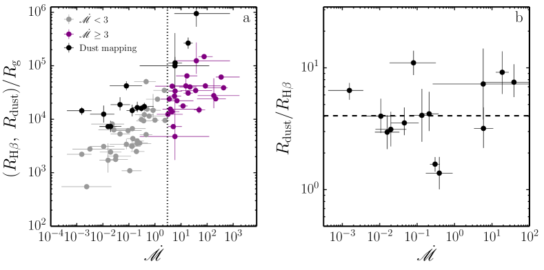
Figure 7: Black hole mass-scaled BLR (purple and grey points) and dust reverberation radii (black points). Panel a shows $R_{\rm dust}/R_{\rm g}$ and $R_{{}_{\rm H\beta}}/R_{\rm g}$ versus $\dot{\mathscr{M}}$. Panel b shows ratios of $R_{\rm dust}/R_{{}_{\rm H\beta}}$ as a function of $\dot{\mathscr{M}}$. Note the large scatter in both low and high $\dot{\mathscr{M}}$ groups.

Figure 7 compares the dust and H$\beta$ radii as a function of $\dot{\mathscr{M}}$ in two different ways. The left panel (7a) shows the dimensionless radii of the BLR and the torus inner walls for 14 objects in the Koshida et al. (2014) sample for which we have measured H$\beta$ lags. The right panel (7b) shows the ratio of the two radii for all these objects. The surprising result is the unexpectedly large scatter in this ratio. While H$\beta$ and the hot dust follow the continuum luminosity in basically an identical way (size proportional to $L^{1/2}$), and differ only in their normalization, this does not result in similar ratios between the two distances for all sources. In fact, the ratios we measure range from about 1.4 for Mrk 590 to about 10 for Mrk 335 and NGC 4593. The median ratio, shown in the diagram, is about 4. The large scatter and the very small number of sources with measured dust lags prevent us from obtaining a meaningful relationship between $R_{\rm dust}$ and $\dot{\mathscr{M}}$.

There are several interesting ideas about the location of the innermost walls of the torus around slim accretion disks (e.g., Kawakatu & Ohsuga 2011; Kawaguchi 2013). In particular, the large attenuation of the slim disk radiation at high polar angles (Wang et al. 2014b) would predict a small $R_{\rm dust}$ at these locations, perhaps as small as the self-gravity radius of the disk. This is not evident in the present data which suggests that the geometry of the inner torus walls is more complicated than the simplistic model suggested in various papers.

5.4 SEAMBHs and Cosmology

The new results presented here suggest that the $R_{{}_{\rm H\beta}}-L_{5100}$ relationship for AGNs requires an additional parameter. In particular, the use of the earlier correlations that are based on low accretion rate sources, tend to over-estimate the BLR size of high$-\dot{\mathscr{M}}$ sources and hence their BH mass. The shorter H$\beta$ lags found here indicate that these objects have smaller BLR size than the ones obtained by applying the old $R_{{}_{\rm H\beta}}-L_{5100}$ relationships. This implies smaller BH mass and, therefore, higher Eddington ratios. Recent work by Kelly & Shen (2013), Nobuta et al. (2012), and Netzer & Trakhtenbrot (2014) all show the large fraction of high $L_{\rm Bol}/L_{\rm Edd}$ sources at high redshifts. This number is likely to increase given the necessary correction to the BH mass found here.

There are several ways of using AGNs for cosmology. These include using the measured diameters of various BLRs (Elvis & Karovska 2002), the empirical $R_{{}_{\rm H\beta}}-L_{5100}$ relation (Horne et al. 2003; Watson et al. 2011; Czerny et al. 2013), torus inner edge reverberation (Yoshii et al. 2014; Hönig et al. 2014), and RMS X-ray spectra (La Franca et al. 2014). The use of SEAMBHs as cosmological distance indicators has been suggested by Wang et al. (2013) and explained in great detail in Paper II where we examined the consequences of increasing $\dot{\mathscr{M}}$ that leads to an almost constant $L_{\rm Bol}/M_{\bullet}$. Marziani & Sulentic (2014) used a similar approach based on a sample of highly accreting AGNs identified by their 4D eigenvector 1 (see also King et al. 2014). While we used RM-based BH mass measurements (Paper II), they used the standard single-epoch method, combined with photoionization modeling, to estimate $R_{{}_{\rm H\beta}}$

The usefulness of the present method for cosmology depends on the number of SEAMBHs with accurately measured $M_{\bullet}$ at high redshifts. As shown above, the reduction in the BLR size in SEAMBHs compared to the size in low accretion rate sources (used so far to estimate BH mass) depends on $\dot{\mathscr{M}}$ and can reach a factor of $3\sim 4$ for $\dot{\mathscr{M}}=100$ (Figure 4a and Equation 7). It is reasonable to expect that higher values of $\dot{\mathscr{M}}$ are associated with an even greater reduction relative to expressions currently used in the literature. At redshifts $z=1\sim 2$, the reduction is more significant than the increase in the measured lag due to the cosmological dilution factor ($1+z$) suggesting that many SEAMBHs at high redshifts, even those with higher luminosity, can be monitored, successfully, and their $R_{{}_{\rm H\beta}}$ measured, during one observing season, given adequate observing facilities.

6 Conclusions

We have completed two years of spectroscopic monitoring of 18 AGNs that are high-accretion candidates. The second year observations resulted in significant H$\beta$ lag measurements of five AGNs, all of which are identified as SEAMBHs. The highest accretion rate reaches $\dot{\mathscr{M}}\gtrsim 200$ in a few objects. The main results of our study can be summarized as follows:

• For a given $L_{5100}$, the SEAMBHs monitored by us generally have shorter H$\beta$ lags by a factor of up to $\sim 3-4$ compared with lower accretion rate AGNs. The reduction gets larger with increasing dimensionless accretion rates.

• We considered several possible explanations for the new results and suggest that they may be related to the strong anisotropy and self-shadowing of the central slim disk radiation. We defined a new radius-mass parameter, $Y=m_{7}^{0.29}r_{{}_{\rm H\beta}}$ and demonstrated that it reaches saturation when the accretion rate exceeds a critical value of $\dot{\mathscr{M}}_{c}=13.8_{-8.1}^{+19.6}$. This transition accretion rate is significantly smaller than the one predicted by classical slim disks model, but is in better agreement with modified slim disk models.

• The shorter H$\beta$ lags imply that the number of SEAMBHs in the universe probably has been underestimated in earlier works that did not take into account the smaller BLR in such sources. It also helps to obtain lag measurements in a shorter time, thus making the application of SEAMBHs to cosmology more feasible.

Our observed sample, combined with SEAMBHs obtained from the literature, is too small to put stronger constraints on the radius-mass saturation parameter. Larger SEAMBH samples with a large dynamic range in $\dot{\mathscr{M}}$, will provide better understanding of the nature of transition from thin to slim disk systems. Better and more accurate BH mass measurements, based on improved numerical tools such as the MCMC technique as applied to velocity-resolved RM observations (Pancoast et al. 2011; Li et al. 2013), will help too. Finally, we are aware of the limitations of the current theory and numerical simulations of slim accretion disks. Present super-Eddington accretion models are still missing important physical ingredients and the observations presented here will be compared with more detailed calculations once these become available.

Table 1: The SEAMBH project: targets and observations

Object	$\alpha_{2000}$	$\delta_{2000}$	redshift	monitoring period	$N_{\rm spec}$	S/N				Comparison stars		Note on $\tau_{{}_{\rm H\beta}}$
						$m_{r^{\prime}}$(Lj)	$m_{r^{\prime}}$(WO)	Spec		$R_{*}$	P.A.
First phase: SEAMBH2012 sample
Mrk 335	00 06 19.5	$+$20 12 10	0.0258	Oct., 2012 $-$ Feb., 2013	91	50	$\cdots$	21		$80^{\prime\prime}.7$	$174.5^{\circ}$	Yes
Mrk 1044	02 30 05.5	$-$08 59 53	0.0165	Oct., 2012 $-$ Feb., 2013	77	91	$\cdots$	21		$207^{\prime\prime}.0$	$-143.0^{\circ}$	Yes
IRAS 04416+1215	04 44 28.8	$+$12 21 12	0.0889	Oct., 2012 $-$ Mar., 2013	92	12	$\cdots$	31		$137^{\prime\prime}.9$	$-55.0^{\circ}$	Yes
Mrk 382	07 55 25.3	$+$39 11 10	0.0337	Oct., 2012 $-$ May., 2013	123	25	$\cdots$	3		$198^{\prime\prime}.4$	$-24.6^{\circ}$	Yes
Mrk 142	10 25 31.3	$+$51 40 35	0.0449	Nov., 2012 $-$ Apr., 2013	119	45	$\cdots$	10		$113^{\prime\prime}.1$	$155.2^{\circ}$	Yes
MCG $+06-26-012$	11 39 13.9	$+$33 55 51	0.0328	Jan., 2013 $-$ Jun., 2013	34	24	$\cdots$	37		$204^{\prime\prime}.3$	$46.1^{\circ}$	Yes
Mrk 42	11 53 41.8	$+$46 12 43	0.0246	Jan., 2013 $-$ Apr., 2013	53	24	$\cdots$	15		$234^{\prime\prime}.4$	$33.8^{\circ}$	No
IRAS F12397+3333	12 42 10.6	$+$33 17 03	0.0435	Jan., 2013 $-$ May., 2013	51	53	$\cdots$	32		$189^{\prime\prime}.0$	$130.0^{\circ}$	Yes
Mrk 486	15 36 38.3	$+$54 33 33	0.0389	Mar., 2013 $-$ Jul., 2013	45	100	$\cdots$	44		$193^{\prime\prime}.8$	$-167.0^{\circ}$	Yes
Mrk 493	15 59 09.6	$+$35 01 47	0.0313	Apr., 2013 $-$ Jun., 2013	27	40	$\cdots$	45		$155^{\prime\prime}.3$	$98.5^{\circ}$	Yes
Second phase: SEAMBH2013 sample
SDSS J075101.42+291419.1	07 51 01.4	$+$29 14 19	0.1208	Nov., 2013 $-$ May., 2014	38	50	50	40		$133^{\prime\prime}.3$	$-41.3^{\circ}$	Yes
SDSS J080101.41+184840.7	08 01 01.4	$+$18 48 40	0.1396	Nov., 2013 $-$ Apr., 2014	34	50	50	50		$118^{\prime\prime}.8$	$-98.2^{\circ}$	Yes
SDSS J080131.58+354436.4	08 01 31.6	$+$35 44 36	0.1786	Nov., 2013 $-$ Apr., 2014	31	50	50	30		$100^{\prime\prime}.0$	$145.2^{\circ}$	uncertain
SDSS J081441.91+212918.5	08 14 41.9	$+$21 29 19	0.1628	Nov., 2013 $-$ May., 2014	34	30	30	30		$79^{\prime\prime}.0$	$73.9^{\circ}$	Yes
SDSS J081456.10+532533.5	08 14 56.1	$+$53 25 34	0.1197	Nov., 2013 $-$ Apr., 2014	27	40	…	50		$164^{\prime\prime}.5$	$-172.9^{\circ}$	Yes
SDSS J093922.89+370943.9	09 39 22.9	$+$37 09 44	0.1859	Nov., 2013 $-$ Jun., 2014	26	40	30	30		$175^{\prime\prime}.1$	$-139.0^{\circ}$	Yes
SDSS J094422.13+103739.7	09 44 22.1	$+$10 37 40	0.2410	Jan., 2014 $-$ Apr., 2014	17	30	30	15		$109^{\prime\prime}.3$	$170.1^{\circ}$	No
SDSS J100055.71+314001.2	10 00 55.7	$+$31 40 01	0.1948	Nov., 2013 $-$ Jun., 2014	26	100	15	40		$151^{\prime\prime}.2$	$116.8^{\circ}$	No

Note. — We denote the samples monitored during the 2012–2013 and 2013–2014 observing seasons as SEAMBH2012 and SEAMBH2013, respectively. The SEAMBH2012 group is described in Papers I, II and III. No observational points were removed from the SEAMBH2012 sample due to S/N ratios. $N_{\rm spec}$ is the numbers of spectroscopic epochs, $R_{*}$ is the angular distance between the object and the comparison star and PA the position angle from the AGN to the comparison star. The last column contains notes on the H$\beta$ time lags: “Yes” means significant lag, “No” lags that could not be measured and “uncertain” refers to the case of J080131 described in the text. $m_{r^{\prime}}$(Lj/WO) are referred to photometry at Lijiang Station of Yunnan Observatory and Wise Observatory. We calculated S/N ratios of the SEAMBH2012 and SEAMBH2013 samples from light curves. We removed those points of SEAMBH2013 sample in poor observing conditions in light of the lowest S/N ratios listed here. Only a few points with extremely large error bars were removed in SEAMBH2012 sample (see details in Papers I and II). Objects marked with “$\cdots$” were not observed at the Wise observatory.

Table 2: Light curves of J075101 and J080101

J075101									J080101
Continuum			Combined Continuum			Line			Continuum			Combined Continuum			Line
JD	$F_{5100}$		JD	$F_{5100}$		JD	$F_{\rm H\beta}$		JD	$F_{5100}$		JD	$F_{5100}$		JD	$F_{\rm H\beta}$
3.466	$6.219\pm 0.169$W		3.466	$6.219\pm 0.169$		10.277	$4.312\pm 0.055$		13.310	$6.835\pm 0.089$L		13.310	$6.835\pm 0.089$		16.257	$6.696\pm 0.076$
8.588	$5.850\pm 0.181$W		8.588	$5.850\pm 0.181$		13.247	$4.413\pm 0.074$		16.257	$7.120\pm 0.051$S		16.257	$7.120\pm 0.051$		21.430	$6.484\pm 0.055$
10.277	$6.325\pm 0.046$S		10.277	$6.325\pm 0.046$		15.248	$4.508\pm 0.091$		21.430	$6.834\pm 0.046$S		21.440	$6.793\pm 0.057$		24.365	$6.294\pm 0.058$
13.247	$6.559\pm 0.075$S		13.256	$6.455\pm 0.146$		22.222	$4.019\pm 0.053$		21.449	$6.753\pm 0.085$L		24.377	$6.803\pm 0.064$		29.270	$6.330\pm 0.051$
13.265	$6.352\pm 0.103$L		15.248	$7.155\pm 0.074$		25.255	$3.699\pm 0.058$		24.365	$6.758\pm 0.076$S		29.283	$6.866\pm 0.060$		33.432	$6.485\pm 0.062$

Note. — JD: Julian dates from 2,456,600; $F_{5100}$ and $F_{\rm H\beta}$ are fluxes at $(1+z)5100$Å  and H$\beta$ emission lines in units of $10^{-16}{\rm erg~{}s^{-1}~{}cm^{-2}~{}\AA^{-1}}$ and $10^{-14}{\rm erg~{}s^{-1}~{}cm^{-2}}$. L: Photometry from Lijiang. S: Spectrum from Lijiang. W: Photometry from Wise. (This table is available in its entirety in a machine-readable form in the online journal. A portion is shown here for guidance regarding its form and content.)

Table 3: Light curves of J080131 and J081441

J080131									J081441
Continuum			Combined Continuum			Line			Continuum			Combined Continuum			Line
JD	$F_{5100}$		JD	$F_{5100}$		JD	$F_{\rm H\beta}$		JD	$F_{5100}$		JD	$F_{5100}$		JD	$F_{\rm H\beta}$
3.478	$2.146\pm 0.072$W		3.478	$2.146\pm 0.072$		6.296	$1.301\pm 0.022$		3.490	$2.720\pm 0.042$W		3.490	$2.720\pm 0.042$		18.318	$2.590\pm 0.054$
6.296	$2.230\pm 0.020$S		6.311	$2.326\pm 0.136$		7.336	$1.318\pm 0.021$		8.612	$2.725\pm 0.036$W		8.612	$2.725\pm 0.036$		23.290	$2.856\pm 0.035$
6.325	$2.422\pm 0.029$L		7.351	$2.258\pm 0.040$		9.343	$1.218\pm 0.020$		18.318	$2.502\pm 0.064$S		18.318	$2.502\pm 0.064$		30.409	$2.782\pm 0.022$
7.336	$2.287\pm 0.015$S		8.600	$2.146\pm 0.068$		12.401	$1.221\pm 0.027$		23.290	$2.599\pm 0.028$S		23.309	$2.626\pm 0.039$		34.369	$2.743\pm 0.028$
7.367	$2.230\pm 0.029$L		9.343	$2.241\pm 0.012$		21.278	$1.175\pm 0.024$		23.328	$2.654\pm 0.097$L		30.409	$2.772\pm 0.010$		37.301	$2.728\pm 0.022$

Note. — This table is available in its entirety in a machine-readable form in the online journal. A portion is shown here for guidance regarding its form and content.

Table 4: Light curves of J081456 and J093922

J081456									J093922
Continuum			Combined Continuum			Line			Continuum			Combined Continuum			Line
JD	$F_{5100}$		JD	$F_{5100}$		JD	$F_{\rm H\beta}$		JD	$F_{5100}$		JD	$F_{5100}$		JD	$F_{\rm H\beta}$
6.344	$6.026\pm 0.028$S		6.349	$6.089\pm 0.090$		6.344	$3.507\pm 0.041$		3.589	$2.673\pm 0.086$W		3.589	$2.673\pm 0.086$		17.372	$1.300\pm 0.033$
6.354	$6.152\pm 0.031$L		7.380	$6.066\pm 0.030$		7.380	$3.441\pm 0.040$		17.372	$2.668\pm 0.014$S		17.372	$2.668\pm 0.014$		66.424	$1.137\pm 0.029$
7.380	$6.066\pm 0.030$S		10.430	$6.083\pm 0.040$		10.422	$3.297\pm 0.039$		50.596	$2.554\pm 0.071$W		50.596	$2.554\pm 0.071$		68.304	$1.070\pm 0.032$
10.422	$6.054\pm 0.030$S		13.346	$6.017\pm 0.046$		19.319	$3.184\pm 0.036$		54.414	$2.377\pm 0.078$W		54.414	$2.377\pm 0.078$		79.421	$1.029\pm 0.038$
10.438	$6.112\pm 0.024$L		19.319	$5.974\pm 0.051$		22.382	$3.026\pm 0.046$		56.441	$2.537\pm 0.076$W		56.441	$2.537\pm 0.076$		81.239	$1.140\pm 0.022$

Note. — This table is available in its entirety in a machine-readable form in the online journal. A portion is shown here for guidance regarding its form and content.

Table 5: Light curves of J094422 and J100055

J094422									J100055
Continuum			Combined Continuum			Line			Continuum			Combined Continuum			Line
JD	$F_{5100}$		JD	$F_{5100}$		JD	$F_{\rm H\beta}$		JD	$F_{5100}$		JD	$F_{5100}$		JD	$F_{\rm H\beta}$
3.614	$1.500\pm 0.038$W		3.614	$1.500\pm 0.038$		62.387	$1.051\pm 0.020$		9.512	$2.921\pm 0.248$W		9.512	$2.921\pm 0.248$		18.388	$0.697\pm 0.040$
9.476	$1.405\pm 0.063$W		9.476	$1.405\pm 0.063$		67.447	$1.043\pm 0.027$		18.388	$3.649\pm 0.042$S		18.388	$3.649\pm 0.042$		44.397	$0.823\pm 0.046$
53.437	$1.157\pm 0.035$W		53.437	$1.157\pm 0.035$		81.351	$1.030\pm 0.029$		43.551	$2.932\pm 0.237$W		43.551	$2.932\pm 0.237$		64.438	$0.747\pm 0.030$
56.469	$1.216\pm 0.040$W		56.469	$1.216\pm 0.040$		84.394	$0.964\pm 0.024$		44.397	$3.483\pm 0.038$S		44.397	$3.483\pm 0.038$		67.261	$0.798\pm 0.029$
61.528	$1.222\pm 0.040$W		61.528	$1.222\pm 0.040$		87.234	$0.961\pm 0.018$		45.611	$3.203\pm 0.265$W		45.611	$3.203\pm 0.265$		71.420	$0.802\pm 0.033$

Note. — This table is available in its entirety in a machine-readable form in the online journal. A portion is shown here for guidance regarding its form and content.

Table 6: H$\beta$ Reverberations of the SEAMBH Targets

Objects	$\tau_{{}_{\rm H\beta}}$	FWHM	$\sigma_{\rm line}$	$\log\left(M_{\bullet}/M_{\odot}\right)$	$\log\dot{\mathscr{M}}$	$\log L_{5100}$	$\log L_{{}_{\rm H\beta}}$	EW(H$\beta$)
	(days)	($\rm km~{}s^{-1}$)	($\rm km~{}s^{-1}$)			($\rm erg~{}s^{-1})$	($\rm erg~{}s^{-1})$	(Å)
SEAMBH2012
Mrk 335	$8.7_{-1.9}^{+1.6}$	$2096\pm 170$	$1470\pm 50$	$6.87_{-0.14}^{+0.10}$	$1.28_{-0.30}^{+0.37}$	$43.69\pm 0.06$	$42.03\pm 0.06$	$110.5\pm 22.3$
Mrk 1044	$10.5_{-2.7}^{+3.3}$	$1178\pm 22$	$766\pm 8$	$6.45_{-0.13}^{+0.12}$	$1.22_{-0.41}^{+0.40}$	$43.10\pm 0.10$	$41.39\pm 0.09$	$101.4\pm 31.9$
Mrk 382	$7.5_{-2.0}^{+2.9}$	$1462\pm 296$	$840\pm 37$	$6.50_{-0.29}^{+0.19}$	$1.18_{-0.53}^{+0.69}$	$43.12\pm 0.08$	$41.01\pm 0.05$	$39.6\pm 9.0$
Mrk 142	$7.9_{-1.1}^{+1.2}$	$1588\pm 58$	$948\pm 12$	$6.59_{-0.07}^{+0.07}$	$1.65_{-0.23}^{+0.23}$	$43.56\pm 0.06$	$41.60\pm 0.04$	$55.2\pm 9.5$
MCG +06-26-012a	$24.0_{-4.8}^{+8.4}$	$1334\pm 80$	$785\pm 21$	$6.92_{-0.12}^{+0.14}$	$-0.34_{-0.45}^{+0.37}$	$42.67\pm 0.11$	$41.03\pm 0.06$	$114.6\pm 32.5$
IRAS F12397b	$9.7_{-1.8}^{+5.5}$	$1802\pm 560$	$1150\pm 122$	$6.79_{-0.45}^{+0.27}$	$2.26_{-0.62}^{+0.98}$	$44.23\pm 0.05$	$42.26\pm 0.04$	$54.2\pm 8.4$
Mrk 486	$23.7_{-2.7}^{+7.5}$	$1942\pm 67$	$1296\pm 23$	$7.24_{-0.06}^{+0.12}$	$0.55_{-0.32}^{+0.20}$	$43.69\pm 0.05$	$42.12\pm 0.04$	$135.9\pm 20.3$
Mrk 493	$11.6_{-2.6}^{+1.2}$	$778\pm 12$	$513\pm 5$	$6.14_{-0.11}^{+0.04}$	$1.88_{-0.21}^{+0.33}$	$43.11\pm 0.08$	$41.35\pm 0.05$	$87.4\pm 18.1$
IRAS 04416c	$13.3_{-1.4}^{+13.9}$	$1522\pm 44$	$1056\pm 29$	$6.78_{-0.06}^{+0.31}$	$2.63_{-0.67}^{+0.16}$	$44.47\pm 0.03$	$42.51\pm 0.02$	$55.8\pm 4.7$
SEAMBH2013
SDSS J075101	$33.4_{-5.6}^{+15.6}$	$1495\pm 67$	$1055\pm 32$	$7.16_{-0.09}^{+0.17}$	$1.34_{-0.41}^{+0.25}$	$44.12\pm 0.05$	$42.25\pm 0.03$	$68.1\pm 8.6$
SDSS J080101	$8.3_{-2.7}^{+9.7}$	$1930\pm 18$	$1119\pm 3$	$6.78_{-0.17}^{+0.34}$	$2.33_{-0.72}^{+0.39}$	$44.27\pm 0.03$	$42.58\pm 0.02$	$105.5\pm 8.3$
SDSS J081441	$18.4_{-8.4}^{+12.7}$	$1615\pm 22$	$1122\pm 11$	$6.97_{-0.27}^{+0.23}$	$1.56_{-0.57}^{+0.63}$	$44.01\pm 0.07$	$42.42\pm 0.03$	$132.0\pm 23.7$
SDSS J081456	$24.3_{-16.4}^{+7.7}$	$2409\pm 61$	$1438\pm 32$	$7.44_{-0.49}^{+0.12}$	$0.59_{-0.30}^{+1.03}$	$43.99\pm 0.04$	$42.15\pm 0.03$	$74.4\pm 7.6$
SDSS J093922	$11.9_{-6.3}^{+2.1}$	$1209\pm 16$	$835\pm 11$	$6.53_{-0.33}^{+0.07}$	$2.54_{-0.20}^{+0.71}$	$44.07\pm 0.04$	$42.09\pm 0.04$	$53.0\pm 6.7$

Note. — 1: H$\beta$ lags of J080131 are not listed in this table, but given in the second paragraph of Section 3 in the main text. 2: All SEAMBH2012 measurements are taken from Paper III, but 5100Å  fluxes are from I and II. ^aMCG +06$-$26$-$012 was selected as a super-Eddington candidate but later was identified to be a sub-Eddington accretor ($\dot{\mathscr{M}}=0.46$). ^bFor IRAS F12397, we use the fluxes of the case with local absorption correction (see the details in Paper I and III). ^c The time lag of IRAS 04416 cannot be obtained significantly using the integration method in Papers I and II, but has been detected by the fitting procedures in Paper III.

Table 7: Reverberation mapping AGNs and results

Objects	$\tau_{{}_{\rm H\beta}}$	FWHM	$\log\left(M_{\bullet}/M_{\odot}\right)$	$\log\dot{\mathscr{M}}$	$\log L_{5100}$	$\log L_{{}_{\rm H\beta}}$	EW(H$\beta$)	Ref.
	(days)	($\rm km~{}s^{-1}$)			($\rm erg~{}s^{-1})$	($\rm erg~{}s^{-1})$	(Å)
Mrk 335	$8.7_{-1.9}^{+1.6}$	$2096\pm 170$	$6.87_{-0.14}^{+0.10}$	$1.17_{-0.30}^{+0.31}$	$43.69\pm 0.06$	$42.03\pm 0.06$	$110.5\pm 22.3$	1,2,3
	$16.8_{-4.2}^{+4.8}$	$1792\pm 3$	$7.02_{-0.12}^{+0.11}$	$1.28_{-0.29}^{+0.30}$	$43.76\pm 0.06$	$42.13\pm 0.06$	$119.7\pm 23.3$	4,5,6,7
	$12.5_{-5.5}^{+6.6}$	$1679\pm 2$	$6.84_{-0.25}^{+0.18}$	$1.39_{-0.29}^{+0.30}$	$43.84\pm 0.06$	$42.18\pm 0.06$	$111.2\pm 21.1$	4,5,6,7
	$14.3_{-0.7}^{+0.7}$	$1724\pm 236$	$6.92_{-0.14}^{+0.11}$	$1.25_{-0.29}^{+0.30}$	$43.74\pm 0.06$	$41.99\pm 0.07$	$89.5\pm 19.5$	4,8a
	$\bm{14.0_{-3.4}^{+4.6}}$	$\bm{1707\pm 79}$	$\bm{6.93_{-0.11}^{+0.10}}$	$\bm{1.27_{-0.17}^{+0.18}}$	$\bm{43.76\pm 0.07}$	$\bm{42.09\pm 0.09}$	$\bm{108.2\pm 16.8}$
PG 0026+129	$111.0_{-28.3}^{+24.1}$	$2544\pm 56$	$8.15_{-0.13}^{+0.09}$	$0.65_{-0.20}^{+0.28}$	$44.97\pm 0.02$	$42.93\pm 0.04$	$46.2\pm 4.7$	4,5,6,9
PG 0052+251	$89.8_{-24.1}^{+24.5}$	$5008\pm 73$	$8.64_{-0.14}^{+0.11}$	$-0.59_{-0.25}^{+0.31}$	$44.81\pm 0.03$	$43.13\pm 0.05$	$107.4\pm 14.8$	4,5,6,9
Fairall9	$17.4_{-4.3}^{+3.2}$	$5999\pm 66$	$8.09_{-0.12}^{+0.07}$	$-0.71_{-0.21}^{+0.31}$	$43.98\pm 0.04$	$42.67\pm 0.04$	$249.8\pm 32.0$	4,5,6,10
Mrk 590	$20.7_{-2.7}^{+3.5}$	$2788\pm 29$	$7.50_{-0.06}^{+0.07}$	$-0.22_{-0.25}^{+0.24}$	$43.59\pm 0.06$	$41.92\pm 0.06$	$107.0\pm 22.0$	4,5,6,7
	$14.0_{-8.8}^{+8.5}$	$3729\pm 426$	$7.58_{-0.48}^{+0.22}$	$-0.91_{-0.30}^{+0.28}$	$43.14\pm 0.09$	$41.58\pm 0.16$	$142.8\pm 62.2$	4,5,6,7
	$29.2_{-5.0}^{+4.9}$	$2744\pm 79$	$7.63_{-0.09}^{+0.07}$	$-0.54_{-0.26}^{+0.25}$	$43.38\pm 0.07$	$41.75\pm 0.07$	$119.7\pm 28.1$	4,5,6,7
	$28.8_{-4.2}^{+3.6}$	$2500\pm 42$	$7.55_{-0.07}^{+0.05}$	$-0.13_{-0.25}^{+0.24}$	$43.65\pm 0.06$	$41.92\pm 0.07$	$94.9\pm 20.7$	4,5,6,7
	$\bm{25.6_{-5.3}^{+6.5}}$	$\bm{2716\pm 202}$	$\bm{7.55_{-0.08}^{+0.07}}$	$\bm{-0.41_{-0.36}^{+0.36}}$	$\bm{43.50\pm 0.21}$	$\bm{41.85\pm 0.12}$	$\bm{108.6\pm 20.2}$
Mrk 1044	$10.5_{-2.7}^{+3.3}$	$1178\pm 22$	$6.45_{-0.13}^{+0.12}$	$1.22_{-0.41}^{+0.40}$	$43.10\pm 0.10$	$41.39\pm 0.09$	$101.4\pm 31.9$	1,2,3
3C 120	$38.1_{-15.3}^{+21.3}$	$2327\pm 48$	$7.61_{-0.22}^{+0.19}$	$0.03_{-0.37}^{+0.37}$	$44.07\pm 0.05$	$42.37\pm 0.06$	$100.9\pm 18.3$	4,5,6,7
	$25.9_{-2.3}^{+2.3}$	$3529\pm 176$	$7.80_{-0.06}^{+0.05}$	$-0.17_{-0.37}^{+0.37}$	$43.94\pm 0.05$	$42.36\pm 0.05$	$135.9\pm 22.3$	4,8a
	$\bm{26.2_{-6.6}^{+8.7}}$	$\bm{2472\pm 729}$	$\bm{7.79_{-0.15}^{+0.15}}$	$\bm{-0.07_{-0.30}^{+0.30}}$	$\bm{44.00\pm 0.10}$	$\bm{42.36\pm 0.04}$	$\bm{118.8\pm 28.9}$
IRAS 04416	$13.3_{-1.4}^{+13.9}$	$1522\pm 44$	$6.78_{-0.06}^{+0.31}$	$2.63_{-0.67}^{+0.16}$	$44.47\pm 0.03$	$42.51\pm 0.02$	$55.8\pm 4.7$	1,2,3
Ark 120	$47.1_{-12.4}^{+8.3}$	$6042\pm 35$	$8.53_{-0.13}^{+0.07}$	$-1.48_{-0.23}^{+0.24}$	$43.98\pm 0.06$	$42.60\pm 0.05$	$211.5\pm 37.5$	4,5,6,7
	$37.1_{-5.4}^{+4.8}$	$6246\pm 78$	$8.45_{-0.07}^{+0.05}$	$-2.01_{-0.27}^{+0.27}$	$43.63\pm 0.08$	$42.43\pm 0.07$	$321.1\pm 77.6$	4,5,6,7
	$\bm{39.5_{-7.8}^{+8.5}}$	$\bm{6077\pm 147}$	$\bm{8.47_{-0.08}^{+0.07}}$	$\bm{-1.70_{-0.41}^{+0.41}}$	$\bm{43.87\pm 0.25}$	$\bm{42.54\pm 0.13}$	$\bm{244.8\pm 80.3}$
Mrk 79	$9.0_{-7.8}^{+8.3}$	$5056\pm 85$	$7.65_{-0.88}^{+0.28}$	$-0.75_{-0.34}^{+0.41}$	$43.63\pm 0.07$	$41.89\pm 0.07$	$92.4\pm 21.0$	4,5,6,7
	$16.1_{-6.6}^{+6.6}$	$4760\pm 31$	$7.85_{-0.23}^{+0.15}$	$-0.59_{-0.34}^{+0.41}$	$43.74\pm 0.07$	$41.92\pm 0.08$	$78.1\pm 18.3$	4,5,6,7
	$16.0_{-5.8}^{+6.4}$	$4766\pm 71$	$7.85_{-0.20}^{+0.15}$	$-0.70_{-0.34}^{+0.41}$	$43.66\pm 0.07$	$41.89\pm 0.07$	$86.0\pm 19.3$	4,5,6,7
	$\bm{15.6_{-4.9}^{+5.1}}$	$\bm{4793\pm 145}$	$\bm{7.84_{-0.16}^{+0.12}}$	$\bm{-0.68_{-0.21}^{+0.25}}$	$\bm{43.68\pm 0.07}$	$\bm{41.90\pm 0.05}$	$\bm{85.4\pm 13.3}$
SDSS J075101	$33.4_{-5.6}^{+15.6}$	$1495\pm 67$	$7.16_{-0.09}^{+0.17}$	$1.34_{-0.41}^{+0.25}$	$44.12\pm 0.05$	$42.25\pm 0.03$	$68.1\pm 8.6$	11
Mrk 382	$7.5_{-2.0}^{+2.9}$	$1462\pm 296$	$6.50_{-0.29}^{+0.19}$	$1.18_{-0.53}^{+0.69}$	$43.12\pm 0.08$	$41.01\pm 0.05$	$39.6\pm 9.0$	1,2,3
SDSS J080101	$8.3_{-2.7}^{+9.7}$	$1930\pm 18$	$6.78_{-0.17}^{+0.34}$	$2.33_{-0.72}^{+0.39}$	$44.27\pm 0.03$	$42.58\pm 0.02$	$105.5\pm 8.3$	11
PG 0804+761	$146.9_{-18.9}^{+18.8}$	$3053\pm 38$	$8.43_{-0.06}^{+0.05}$	$0.00_{-0.13}^{+0.15}$	$44.91\pm 0.02$	$43.29\pm 0.03$	$122.5\pm 10.3$	4,5,6,9
SDSS J081441	$18.4_{-8.4}^{+12.7}$	$1615\pm 22$	$6.97_{-0.27}^{+0.23}$	$1.56_{-0.57}^{+0.63}$	$44.01\pm 0.07$	$42.42\pm 0.03$	$132.0\pm 23.7$	11
SDSS J081456	$24.3_{-16.4}^{+7.7}$	$2409\pm 61$	$7.44_{-0.49}^{+0.12}$	$0.59_{-0.30}^{+1.03}$	$43.99\pm 0.04$	$42.15\pm 0.03$	$74.4\pm 7.6$	11
PG 0844+349	$32.3_{-13.4}^{+13.7}$	$2694\pm 58$	$7.66_{-0.23}^{+0.15}$	$0.50_{-0.42}^{+0.57}$	$44.22\pm 0.07$	$42.56\pm 0.05$	$111.2\pm 22.1$	5,6,9,12
Mrk 110	$24.3_{-8.3}^{+5.5}$	$1543\pm 5$	$7.05_{-0.18}^{+0.09}$	$0.81_{-0.32}^{+0.35}$	$43.68\pm 0.04$	$42.12\pm 0.05$	$139.6\pm 20.4$	4,5,6,7
	$20.4_{-6.3}^{+10.5}$	$1658\pm 3$	$7.04_{-0.16}^{+0.18}$	$0.92_{-0.32}^{+0.34}$	$43.75\pm 0.04$	$42.02\pm 0.05$	$94.8\pm 14.7$	4,5,6,7
	$33.3_{-10.0}^{+14.9}$	$1600\pm 39$	$7.22_{-0.16}^{+0.16}$	$0.58_{-0.33}^{+0.35}$	$43.53\pm 0.05$	$41.97\pm 0.04$	$139.4\pm 20.5$	4,5,6,7
	$\bm{25.6_{-7.2}^{+8.9}}$	$\bm{1634\pm 83}$	$\bm{7.10_{-0.14}^{+0.13}}$	$\bm{0.77_{-0.25}^{+0.26}}$	$\bm{43.66\pm 0.12}$	$\bm{42.03\pm 0.08}$	$\bm{123.8\pm 29.1}$
SDSS J093922	$11.9_{-6.3}^{+2.1}$	$1209\pm 16$	$6.53_{-0.33}^{+0.07}$	$2.54_{-0.20}^{+0.71}$	$44.07\pm 0.04$	$42.09\pm 0.04$	$53.0\pm 6.7$	11
PG 0953+414	$150.1_{-22.6}^{+21.6}$	$3071\pm 27$	$8.44_{-0.07}^{+0.06}$	$0.39_{-0.14}^{+0.16}$	$45.19\pm 0.01$	$43.29\pm 0.04$	$64.7\pm 5.9$	4,5,6,9
NGC 3227	$3.8_{-0.8}^{+0.8}$	$4112\pm 206$	$7.09_{-0.12}^{+0.09}$	$-1.34_{-0.36}^{+0.38}$	$42.24\pm 0.11$	$40.38\pm 0.10$	$71.0\pm 23.6$	4,13a
Mrk 142	$7.9_{-1.1}^{+1.2}$	$1588\pm 58$	$6.59_{-0.07}^{+0.07}$	$1.90_{-0.86}^{+0.85}$	$43.56\pm 0.06$	$41.60\pm 0.04$	$55.2\pm 9.5$	1,2,3
	$2.7_{-0.8}^{+0.7}$	$1462\pm 2$	$6.06_{-0.16}^{+0.10}$	$1.96_{-0.82}^{+0.82}$	$43.61\pm 0.04$	$41.66\pm 0.05$	$57.6\pm 8.6$	4,14
	$\bm{6.4_{-3.4}^{+7.3}}$	$\bm{1462\pm 86}$	$\bm{6.47_{-0.38}^{+0.38}}$	$\bm{1.93_{-0.59}^{+0.59}}$	$\bm{43.59\pm 0.04}$	$\bm{41.62\pm 0.06}$	$\bm{56.6\pm 6.6}$
NGC 3516	$11.7_{-1.5}^{+1.0}$	$5384\pm 269$	$7.82_{-0.08}^{+0.05}$	$-1.97_{-0.52}^{+0.41}$	$42.79\pm 0.20$	$41.06\pm 0.18$	$94.7\pm 59.2$	4,13a
SBS 1116+583A	$2.3_{-0.5}^{+0.6}$	$3668\pm 186$	$6.78_{-0.12}^{+0.11}$	$-0.87_{-0.71}^{+0.51}$	$42.14\pm 0.23$	$40.70\pm 0.07$	$186.8\pm 104.1$	4,14
Arp 151	$4.0_{-0.7}^{+0.5}$	$3098\pm 69$	$6.87_{-0.08}^{+0.05}$	$-0.44_{-0.28}^{+0.30}$	$42.55\pm 0.10$	$40.95\pm 0.11$	$130.0\pm 44.4$	4,14
NGC 3783	$10.2_{-2.3}^{+3.3}$	$3770\pm 68$	$7.45_{-0.11}^{+0.12}$	$-1.58_{-0.59}^{+0.45}$	$42.56\pm 0.18$	$41.01\pm 0.18$	$144.0\pm 83.7$	4,5,6,15
MCG +06-26-012	$24.0_{-4.8}^{+8.4}$	$1334\pm 80$	$6.92_{-0.12}^{+0.14}$	$-0.34_{-0.45}^{+0.37}$	$42.67\pm 0.11$	$41.03\pm 0.06$	$114.6\pm 32.5$	1,2,3
Mrk 1310	$3.7_{-0.6}^{+0.6}$	$2409\pm 24$	$6.62_{-0.08}^{+0.07}$	$-0.31_{-0.39}^{+0.35}$	$42.29\pm 0.14$	$40.56\pm 0.10$	$94.3\pm 38.2$	4,14
NGC 4051	$1.9_{-0.5}^{+0.5}$	$851\pm 277$	$5.42_{-0.53}^{+0.23}$	$1.59_{-0.84}^{+1.29}$	$41.96\pm 0.19$	$40.19\pm 0.18$	$86.8\pm 51.7$	4,13a
NGC 4151	$6.6_{-0.8}^{+1.1}$	$6371\pm 150$	$7.72_{-0.06}^{+0.07}$	$-2.81_{-0.57}^{+0.37}$	$42.09\pm 0.21$	$40.56\pm 0.20$	$150.8\pm 100.6$	4,5,6,16
PG 1211+143	$93.8_{-42.1}^{+25.6}$	$2012\pm 37$	$7.87_{-0.26}^{+0.11}$	$0.84_{-0.35}^{+0.63}$	$44.73\pm 0.08$	$43.02\pm 0.06$	$100.2\pm 22.9$	5,6,9,12
Mrk 202	$3.0_{-1.1}^{+1.7}$	$1471\pm 18$	$6.11_{-0.20}^{+0.20}$	$0.66_{-0.65}^{+0.59}$	$42.26\pm 0.14$	$40.40\pm 0.09$	$70.6\pm 27.5$	4,14
NGC 4253	$6.2_{-1.2}^{+1.6}$	$1609\pm 39$	$6.49_{-0.10}^{+0.10}$	$0.36_{-0.42}^{+0.36}$	$42.57\pm 0.12$	$40.77\pm 0.12$	$81.1\pm 31.6$	4,14
PG 1226+023	$306.8_{-90.9}^{+68.5}$	$3509\pm 36$	$8.87_{-0.15}^{+0.09}$	$0.70_{-0.20}^{+0.33}$	$45.96\pm 0.02$	$44.13\pm 0.04$	$74.6\pm 6.9$	4,5,6,9
PG 1229+204	$37.8_{-15.3}^{+27.6}$	$3828\pm 54$	$8.03_{-0.23}^{+0.24}$	$-1.03_{-0.55}^{+0.52}$	$43.70\pm 0.05$	$42.31\pm 0.06$	$209.7\pm 38.3$	4,5,6,9
NGC 4593	$3.7_{-0.8}^{+0.8}$	$5143\pm 16$	$7.28_{-0.10}^{+0.08}$	$-0.73_{-0.52}^{+0.41}$	$42.87\pm 0.18$	$41.17\pm 0.18$	$101.6\pm 59.0$	4,6,17
	$4.3_{-0.8}^{+1.3}$	$4395\pm 362$	$7.21_{-0.12}^{+0.13}$	$-1.47_{-0.52}^{+0.41}$	$42.38\pm 0.18$	$40.73\pm 0.18$	$115.4\pm 67.6$	18b
	$\bm{4.0_{-0.7}^{+0.8}}$	$\bm{5142\pm 572}$	$\bm{7.26_{-0.09}^{+0.09}}$	$\bm{-1.10_{-0.64}^{+0.60}}$	$\bm{42.62\pm 0.37}$	$\bm{40.95\pm 0.33}$	$\bm{108.3\pm 45.7}$
IRAS F12397	$9.7_{-1.8}^{+5.5}$	$1802\pm 560$	$6.79_{-0.45}^{+0.27}$	$2.26_{-0.62}^{+0.98}$	$44.23\pm 0.05$	$42.26\pm 0.04$	$54.2\pm 8.4$	1,2,3c
NGC 4748	$5.5_{-2.2}^{+1.6}$	$1947\pm 66$	$6.61_{-0.23}^{+0.11}$	$0.10_{-0.44}^{+0.61}$	$42.56\pm 0.12$	$40.98\pm 0.10$	$136.8\pm 50.1$	4,14
PG 1307+085	$105.6_{-46.6}^{+36.0}$	$5059\pm 133$	$8.72_{-0.26}^{+0.13}$	$-0.68_{-0.28}^{+0.53}$	$44.85\pm 0.02$	$43.13\pm 0.06$	$98.4\pm 15.1$	4,5,6,9
NGC 5273	$2.2_{-1.6}^{+1.2}$	$5688\pm 163$	$7.14_{-0.56}^{+0.19}$	$-2.50_{-0.67}^{+1.33}$	$41.54\pm 0.16$	$39.74\pm 0.11$	$82.2\pm 37.1$	19
Mrk 279	$16.7_{-3.9}^{+3.9}$	$5354\pm 32$	$7.97_{-0.12}^{+0.09}$	$-0.89_{-0.30}^{+0.33}$	$43.71\pm 0.07$	$42.12\pm 0.06$	$132.2\pm 28.7$	4,5,6,20
PG 1411+442	$124.3_{-61.7}^{+61.0}$	$2801\pm 43$	$8.28_{-0.30}^{+0.17}$	$-0.23_{-0.38}^{+0.63}$	$44.56\pm 0.02$	$42.85\pm 0.03$	$99.7\pm 8.2$	4,5,6,9
NGC 5548	$19.7_{-1.5}^{+1.5}$	$4674\pm 63$	$7.92_{-0.04}^{+0.03}$	$-1.62_{-0.49}^{+0.46}$	$43.39\pm 0.10$	$41.79\pm 0.10$	$128.1\pm 40.3$	4,5,6,21
	$18.6_{-2.3}^{+2.1}$	$5418\pm 107$	$8.03_{-0.06}^{+0.05}$	$-1.99_{-0.51}^{+0.47}$	$43.14\pm 0.11$	$41.61\pm 0.13$	$151.3\pm 57.9$	4,5,6,21
	$15.9_{-2.5}^{+2.9}$	$5236\pm 87$	$7.93_{-0.08}^{+0.07}$	$-1.68_{-0.49}^{+0.45}$	$43.35\pm 0.09$	$41.72\pm 0.10$	$119.7\pm 37.9$	4,5,6,21
	$11.0_{-2.0}^{+1.9}$	$5986\pm 95$	$7.89_{-0.09}^{+0.07}$	$-2.10_{-0.52}^{+0.47}$	$43.07\pm 0.11$	$41.52\pm 0.17$	$144.5\pm 66.7$	4,5,6,21
	$13.0_{-1.4}^{+1.6}$	$5930\pm 42$	$7.95_{-0.05}^{+0.05}$	$-1.72_{-0.49}^{+0.46}$	$43.32\pm 0.10$	$41.75\pm 0.09$	$135.9\pm 41.2$	4,5,6,21
	$13.4_{-4.3}^{+3.8}$	$7378\pm 39$	$8.15_{-0.17}^{+0.11}$	$-1.64_{-0.49}^{+0.45}$	$43.38\pm 0.09$	$41.73\pm 0.10$	$114.4\pm 37.0$	4,5,6,21
	$21.7_{-2.6}^{+2.6}$	$6946\pm 79$	$8.31_{-0.06}^{+0.05}$	$-1.43_{-0.48}^{+0.45}$	$43.52\pm 0.09$	$41.82\pm 0.09$	$102.4\pm 30.2$	4,5,6,21
	$16.4_{-1.1}^{+1.2}$	$6623\pm 93$	$8.15_{-0.03}^{+0.03}$	$-1.56_{-0.48}^{+0.45}$	$43.43\pm 0.09$	$41.75\pm 0.10$	$106.3\pm 33.3$	4,5,6,21
	$17.5_{-1.6}^{+2.0}$	$6298\pm 65$	$8.13_{-0.04}^{+0.05}$	$-1.85_{-0.49}^{+0.46}$	$43.24\pm 0.10$	$41.72\pm 0.10$	$153.5\pm 50.7$	4,5,6,21
	$26.5_{-2.2}^{+4.3}$	$6177\pm 36$	$8.30_{-0.04}^{+0.07}$	$-1.33_{-0.48}^{+0.45}$	$43.59\pm 0.09$	$41.87\pm 0.10$	$98.1\pm 30.0$	4,5,6,21
	$24.8_{-3.0}^{+3.2}$	$6247\pm 57$	$8.28_{-0.06}^{+0.05}$	$-1.45_{-0.48}^{+0.45}$	$43.51\pm 0.09$	$41.83\pm 0.09$	$106.6\pm 31.5$	4,5,6,21
	$6.5_{-3.7}^{+5.7}$	$6240\pm 77$	$7.69_{-0.37}^{+0.27}$	$-2.04_{-0.51}^{+0.47}$	$43.11\pm 0.11$	$41.64\pm 0.13$	$172.8\pm 66.1$	4,5,6,21
	$14.3_{-7.3}^{+5.9}$	$6478\pm 108$	$8.07_{-0.31}^{+0.15}$	$-2.03_{-0.51}^{+0.47}$	$43.11\pm 0.11$	$41.55\pm 0.14$	$139.8\pm 55.7$	4,5,6,21
	$6.3_{-2.3}^{+2.6}$	$6396\pm 167$	$7.70_{-0.20}^{+0.15}$	$-2.27_{-0.55}^{+0.49}$	$42.96\pm 0.13$	$41.12\pm 0.10$	$74.4\pm 27.3$	4,22
	$4.2_{-1.3}^{+0.9}$	$12771\pm 71$	$8.12_{-0.16}^{+0.08}$	$-2.19_{-0.51}^{+0.47}$	$43.01\pm 0.11$	$41.33\pm 0.10$	$105.3\pm 35.4$	4,14
	$12.4_{-3.9}^{+2.7}$	$11481\pm 574$	$8.50_{-0.17}^{+0.09}$	$-2.21_{-0.53}^{+0.48}$	$42.99\pm 0.11$	$41.27\pm 0.10$	$96.6\pm 34.4$	4,13a
	$\bm{17.6_{-4.7}^{+6.4}}$	$\bm{7241\pm 2200}$	$\bm{8.10_{-0.16}^{+0.16}}$	$\bm{-1.80_{-0.33}^{+0.33}}$	$\bm{43.29\pm 0.20}$	$\bm{41.64\pm 0.23}$	$\bm{117.2\pm 25.9}$
PG 1426+015	$95.0_{-37.1}^{+29.9}$	$7113\pm 160$	$8.97_{-0.22}^{+0.12}$	$-1.51_{-0.28}^{+0.47}$	$44.63\pm 0.02$	$42.83\pm 0.04$	$80.1\pm 9.2$	4,5,6,9
Mrk 817	$19.0_{-3.7}^{+3.9}$	$4711\pm 49$	$7.92_{-0.09}^{+0.08}$	$-0.81_{-0.35}^{+0.35}$	$43.79\pm 0.05$	$42.07\pm 0.05$	$98.0\pm 16.5$	4,5,6,7
	$15.3_{-3.5}^{+3.7}$	$5237\pm 67$	$7.91_{-0.11}^{+0.09}$	$-0.98_{-0.35}^{+0.35}$	$43.67\pm 0.05$	$42.00\pm 0.06$	$108.5\pm 20.4$	4,5,6,7
	$33.6_{-7.6}^{+6.5}$	$4767\pm 72$	$8.17_{-0.11}^{+0.08}$	$-0.98_{-0.35}^{+0.35}$	$43.67\pm 0.05$	$41.92\pm 0.05$	$91.1\pm 15.3$	4,5,6,7
	$14.0_{-3.5}^{+3.4}$	$5627\pm 30$	$7.94_{-0.12}^{+0.09}$	$-0.73_{-0.35}^{+0.35}$	$43.84\pm 0.05$	$41.77\pm 0.05$	$43.2\pm 7.1$	4,13
	$\bm{19.9_{-6.7}^{+9.9}}$	$\bm{5348\pm 536}$	$\bm{7.99_{-0.14}^{+0.14}}$	$\bm{-0.87_{-0.22}^{+0.22}}$	$\bm{43.74\pm 0.09}$	$\bm{41.93\pm 0.14}$	$\bm{78.5\pm 34.3}$
Mrk 1511	$5.7_{-0.8}^{+0.9}$	$4171\pm 137$	$7.29_{-0.07}^{+0.07}$	$-0.34_{-0.24}^{+0.24}$	$43.16\pm 0.06$	$41.52\pm 0.06$	$115.5\pm 23.1$	18b
Mrk 290	$8.7_{-1.0}^{+1.2}$	$4543\pm 227$	$7.55_{-0.07}^{+0.07}$	$-0.85_{-0.23}^{+0.23}$	$43.17\pm 0.06$	$41.64\pm 0.06$	$153.0\pm 29.0$	4,13a
Mrk 486	$23.7_{-2.7}^{+7.5}$	$1942\pm 67$	$7.24_{-0.06}^{+0.12}$	$0.55_{-0.32}^{+0.20}$	$43.69\pm 0.05$	$42.12\pm 0.04$	$135.9\pm 20.3$	1,2,3
Mrk 493	$11.6_{-2.6}^{+1.2}$	$778\pm 12$	$6.14_{-0.11}^{+0.04}$	$1.88_{-0.21}^{+0.33}$	$43.11\pm 0.08$	$41.35\pm 0.05$	$87.4\pm 18.1$	1,2,3
PG 1613+658	$40.1_{-15.2}^{+15.0}$	$9074\pm 103$	$8.81_{-0.21}^{+0.14}$	$-0.97_{-0.31}^{+0.45}$	$44.77\pm 0.02$	$43.00\pm 0.03$	$86.7\pm 7.6$	4,5,6,9
PG 1617+175	$71.5_{-33.7}^{+29.6}$	$6641\pm 190$	$8.79_{-0.28}^{+0.15}$	$-1.50_{-0.33}^{+0.58}$	$44.39\pm 0.02$	$42.74\pm 0.05$	$114.8\pm 15.1$	4,5,6,9
PG 1700+518	$251.8_{-38.8}^{+45.9}$	$2252\pm 85$	$8.40_{-0.08}^{+0.08}$	$1.08_{-0.17}^{+0.17}$	$45.59\pm 0.01$	$43.78\pm 0.02$	$78.9\pm 4.5$	4,5,6,9
3C 390.3	$23.6_{-6.7}^{+6.2}$	$12694\pm 13$	$8.87_{-0.15}^{+0.10}$	$-3.35_{-0.65}^{+0.60}$	$43.68\pm 0.10$	$42.29\pm 0.05$	$206.2\pm 50.7$	4,5,6,23
	$46.4_{-3.2}^{+3.6}$	$13211\pm 28$	$9.20_{-0.03}^{+0.03}$	$-2.12_{-0.51}^{+0.51}$	$44.50\pm 0.03$	$42.78\pm 0.04$	$97.1\pm 10.0$	4,24
	$\bm{44.5_{-17.0}^{+27.6}}$	$\bm{12796\pm 361}$	$\bm{9.18_{-0.23}^{+0.23}}$	$\bm{-2.62_{-0.96}^{+0.95}}$	$\bm{44.43\pm 0.58}$	$\bm{42.60\pm 0.35}$	$\bm{108.8\pm 58.8}$
KA 1858+4850	$13.5_{-2.3}^{+2.0}$	$1820\pm 79$	$6.94_{-0.09}^{+0.07}$	$0.75_{-0.21}^{+0.25}$	$43.43\pm 0.05$	$41.89\pm 0.04$	$146.9\pm 21.1$	25d
NGC 6814	$6.6_{-0.9}^{+0.9}$	$3323\pm 7$	$7.16_{-0.06}^{+0.05}$	$-1.64_{-0.80}^{+0.46}$	$42.12\pm 0.28$	$40.50\pm 0.28$	$121.6\pm 112.2$	4,14
Mrk 509	$79.6_{-5.4}^{+6.1}$	$3015\pm 2$	$8.15_{-0.03}^{+0.03}$	$-0.52_{-0.14}^{+0.13}$	$44.19\pm 0.05$	$42.61\pm 0.04$	$132.7\pm 19.1$	4,5,6,7
PG 2130+099	$9.6_{-1.2}^{+1.2}$	$2450\pm 188$	$7.05_{-0.10}^{+0.08}$	$1.69_{-0.20}^{+0.23}$	$44.20\pm 0.03$	$42.65\pm 0.03$	$142.1\pm 13.6$	4,8a
NGC 7469e	$10.8_{-1.3}^{+3.4}$	$4369\pm 6$	$7.60_{-0.06}^{+0.12}$	$0.90_{-1.87}^{+1.83}$	$43.51\pm 0.11$	$41.60\pm 0.10$	$63.0\pm 21.0$	4,26
	$4.5_{-0.8}^{+0.7}$	$1722\pm 30$	$6.42_{-0.09}^{+0.06}$	$0.63_{-1.90}^{+1.85}$	$43.32\pm 0.12$	$41.71\pm 0.09$	$124.9\pm 44.3$	27,5
	$\bm{6.5_{-3.0}^{+5.8}}$	$\bm{4343\pm 2859}$	$\bm{6.92_{-0.84}^{+0.84}}$	$\bm{0.76_{-1.35}^{+1.31}}$	$\bm{43.43\pm 0.15}$	$\bm{41.66\pm 0.10}$	$\bm{86.9\pm 47.1}$

Note. — Ref: 1. Paper I; 2. Paper II; 3. Paper III; 4. Bentz et al. (2013); 5. Collin et al. (2006); 6. Kaspi et al. (2005); 7. Peterson et al. (1998); 8. Grier et al. (2012); 9. Kaspi et al. (2000); 10. Santos-Lleo et al. (1997); 11. This paper; 12. Bentz et al. (2009a); 13. Denney et al. (2010); 14. Bentz et al. (2009b); 15. Stirpe et al. (1994); 16. Bentz et al. (2006); 17. Denney et al. (2006); 18. Barth et al. (2013); 19. Bentz et al. (2014); 20. Santos-Lleo et al. (2001); 21. Peterson et al. (2002) and references therein; 22. Bentz et al. (2007); 23. Dietrich et al. (1998); 24. Dietrich et al. (2012); 25. Pei et al. (2014); 26. Peterson et al. (2014); 27. Collier et al. (1998).

Superscript $a$ means that the literature does not provide FWHMs from mean spectra or H$\beta$ fluxes with narrow-line components subtracted. For these, we scanned and digitized the mean spectra from the papers, then calculated those numbers ourselves. $b$ means that the AGN continuum is obtained through spectral fitting decomposition (Ref. 18). $c$ for IRAS F12397, we use fluxes for the case with local absorption correction (see the details in Papers I and III). $d$ means that the contribution of host galaxy is provided in Ref. 25. $e$ the virial products of the two independent campaigns are quite different, yielding a large error bars on the mean $M_{\bullet}$ and $\dot{\mathscr{M}}$. In Appendix B, NGC 7469 is shown as an SEAMBH from Collier et al. (1988) and Peterson et al. (2014). Both campaigns have high quality data. Numbers in boldface are the weighted averages of all the measurements of this object. The details of the average scheme are given in the main text.

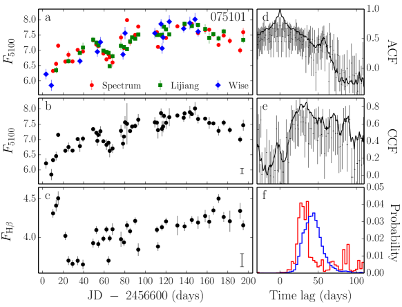
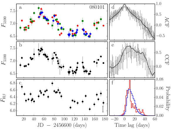
Figure 1: Light curves and cross correlation results. Each object has six panels: (a, b, c) are light curves of the inter-calibrated continuum, combined 5100Å  continuum, and H$\beta$ emissions, respectively; (d, e, f) are auto correlation function (ACF) of the combined continuum, cross correlation function (CCF) of the combined continuum and H$\beta$ emission and the Monte-Carlo simulations of peaks (red) and centroid (blue) of lags, respectively. In panels d and e, the solid lines show the results of ICCF method and the points with error bars are from ZDCF ($Z-$transformed discrete correlation function). $F_{5100}$ and $F_{\rm H\beta}$ are in unit of $10^{-16}{\rm erg~{}s^{-1}~{}cm^{-2}\AA^{-1}}$ and $10^{-14}{\rm erg~{}s^{-1}~{}cm^{-2}}$ for all quasars, respectively. In panel (a) of J075101, the red dots, green squares and blue diamonds are fluxes from Lijiang spectroscopy, photometry and Wise photometry, respectively. The colour points in other objects have the same meanings with that of J075101. Bars with terminals as systematic errors are plotted in the corners of the panels (see Paper I for details).

Figure 1 continued.

Figure 1 continued.

Figure 1 continued.

Figure 1 continued.

Figure 3: The $R_{{}_{\rm H\beta}}-L_{5100}$ and $R_{{}_{\rm H\beta}}-L_{{}_{\rm H\beta}}$ relationships (panel a, c, e) and the deviations of $R_{{}_{\rm H\beta}}$ from the regression relationships (panel b, d, f). The dotted is the fit for the $\dot{\mathscr{M}}<3$ sample whereas the dashed is the fit for the $\dot{\mathscr{M}}>3$ sample in all panels. Panels (a, b) show the comparison of the previous sample and the SEAMBH campaigns. Clearly SEAMBHs are below the $R_{{}_{\rm H\beta}}-L_{5100}$ relation, and the scatter of the relation increases with the inclusion of the SEAMBH2012/2013 samples (see the intrinsic scatter given by the numbers below Equations 4 and 5). Panel b shows $\Delta R_{\rm H\beta}=\log\left(R_{{}_{\rm H\beta}}/R_{{}_{{\rm H\beta},R-L}}\right)$, where $R_{{}_{{\rm H\beta},R-L}}$ is given by Equation (4b). Panels (c,d) show the two samples of $\dot{\mathscr{M}}\geq 3$ and $\dot{\mathscr{M}}<3$ AGNs with averaged RM values for the $R_{{}_{\rm H\beta}}-L_{5100}$ relation and the residual of $\Delta R_{{}_{\rm H\beta}}$, where $R_{{}_{{\rm H\beta},R-L}}$ is given by Equation 5b. Panels (e, f) show the $R_{{}_{\rm H\beta}}-L_{{}_{\rm H\beta}}$ and $\Delta R_{{}_{\rm H\beta}}-\dot{\mathscr{M}}$ relations.

Figure 6: Determination of the saturated$-Y$ and the transition accretion rate. We find $Y\propto\dot{\mathscr{M}}^{0.27\pm 0.04}$, supporting the SS73 disk model below $\dot{\mathscr{M}}_{c}$ and saturation beyond the numbers listed inside the panel supporting the idea of slim accretion disks in SEAMBHs. The outlier with large error bars is NGC 7469 (see Table 7).

Appendix A Mean and RMS spectra

To supplement the material presented in the body of the paper, we provide in Figure 8 the mean and RMS spectra of the objects in the SEAMBH2013 sample calculated by the standard method (e.g., Peterson et al. 2004). Prior to the calculation of these spectra, we corrected the data for the slight wavelength shift caused by the relatively wide aperture used in 2013 ($5^{\prime\prime}$) using the [O iii]$\lambda 5007$ line as our wavelength reference. We define

$$\overline{F}(\lambda)=\frac{1}{N}\sum_{i=1}^{N}F_{i}(\lambda)\,,$$ (A1)

and

$$S(\lambda)=\left\{\frac{1}{N}\sum_{i=1}^{N}\left[F_{i}(\lambda)-\overline{F}(\lambda)\right]^{2}\right\}^{1/2},$$ (A2)

where $F_{i}(\lambda)$ is the $i-$th spectrum and $N$ the total number of spectra obtained during the campaign. The line dispersion is

$$\sigma_{\rm line}^{2}(\lambda)=\langle\lambda^{2}\rangle-\lambda_{0}^{2},$$ (A3)

where $\lambda_{0}=\int\lambda P(\lambda)d\lambda/\int P(\lambda)d\lambda,$ $\langle\lambda^{2}\rangle=\int\lambda^{2}P(\lambda)d\lambda/\int P(\lambda)d\lambda,$ and $P(\lambda)$ is the line profile. The calculated values of $\sigma_{\rm line}$ are listed in Table 6.

Appendix B $R_{{}_{\rm H\beta}}$ Correlations using the direct method

The correlations listed in the main body of the paper were calculated using the average scheme where each object is represented by one point. The results shown in this section are for the direct scheme, where each observing campaign is represented by one point.

The following equations correspond to Equation (6)

$$(1.29\pm 0.02)+(0.52\pm 0.03)\log L_{\rm H\beta,42} ({\rm entire~{}sample}),$$ (B1a)

$$(1.35\pm 0.03)+(0.53\pm 0.03)\log L_{\rm H\beta,42} (\dot{\mathscr{M}}<3),$$ (B1b)

$$(1.17\pm 0.05)+(0.55\pm 0.06)\log L_{\rm H\beta,42} (\dot{\mathscr{M}}\geq 3),$$ (B1c)

with scatters of $\sigma_{\rm in}=(0.20,0.15,0.24)$ for (B1a,B1b,B1c), respectively. For $\Delta R_{{}_{\rm H\beta}}-\dot{\mathscr{M}}$ relation, we have

$$\Delta R_{{}_{\rm H\beta}}=(0.49\pm 0.14)-(0.58\pm 0.10)\log\dot{\mathscr{M}}~{}~{}~{}({\rm for~{}\dot{\mathscr{M}}\geq 3}),$$ (B2)

and

$$\Delta R_{{}_{\rm H\beta}}=(0.44\pm 0.15)-(0.49\pm 0.11)\log\dot{\mathscr{M}}~{}~{}~{}({\rm for~{}\dot{\mathscr{M}}\geq 3}),$$ (B3)

with $\sigma_{\rm in}=(0.01,0.11)$ for deviations from $R_{{}_{\rm H\beta}}-L_{5100}$ and $R_{{}_{\rm H\beta}}-L_{{}_{\rm H\beta}}$ relations, respectively. These correlations are shown in Figures 9 and 10.

For the $Y-\dot{\mathscr{M}}$ relation as shown by Figure 11, we obtained

$$\dot{\mathscr{M}}_{c}=10.8_{-5.7}^{+12.0},~{}~{}Y_{\rm sat}=3.0_{-0.4}^{+0.4}\times 10^{4},~{}~{}{\rm and}~{}~{}k_{0}=0.28\pm 0.03,$$ (B4)

from Figure 12, yielding the critical radius of

$$r_{{}_{\rm H\beta}}=3.0^{+0.4}_{-0.4}\times 10^{4}~{}m_{7}^{0.29};~{}~{}{\rm or}~{}~{}R_{\rm crit}({\rm H\beta})=17.1^{+2.3}_{-2.3}~{}m_{7}^{1.29}~{}{\rm ltd}.$$ (B5)

The results are very similar, and entirely consistent with the results of the average scheme presented in the main body of the paper.

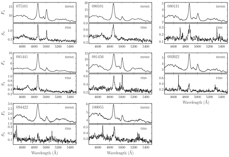
Figure 8: Mean and RMS spectra (observed flux vs. rest-frame wavelength) of the objects in the SEAMBH2013 group.

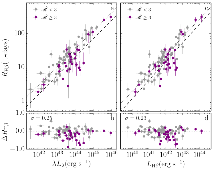
Figure 9: Same as Figure 3 but for the direct scheme. The left panel and Figure 3a are identical, the right panel corresponds to Figure 3e.

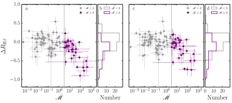
Figure 10: Same as Figure 4 but for the direct scheme. The object with the largest error bar is NGC 7469.

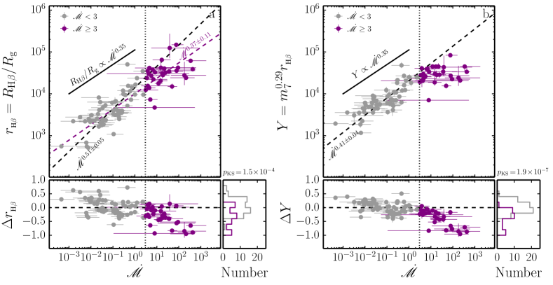
Figure 11: Same as Figure 5 but for the direct scheme.

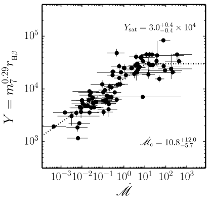
Figure 12: Same as Figure 6 for the direct scheme.

References

- (1) Abramowicz, M. A., Czerny, B., Lasota, J.-P., & Szuszkiewicz, E. 1988, ApJ, 332, 646
- (2) Abramowicz, M. A., Horák, J. & Kluźniak, W. 2013, AcA, 63, 267
- (3) Ade, P. A. R., Aghanim, N., Armitage-Caplan, C. et al. 2014, A&A, 571, 16
- (4) Akritas, M. G. & Bershady, M. A. 1996, ApJ, 470, 706
- (5) Bahcall, J., Kozlovsky, B.-Z. & Salpeter, E. E. 1972, ApJ, 171, 467
- (6) Bardeen, J. M., Press, W. H. & Teukolsky, S. A. 1972, ApJ, 178, 347
- (7) Barth, A. J., Bennert, V. N., Canalizo, G. et al. 2015, ApJ, in press, arXiv:1503.01146
- (8) Barth, A. J., Pancoast, A., Bennert, V. N. et al. 2013, ApJ, 769, 128
- (9) Barvainis, R. 1987, ApJ, 320, 537
- (10) Bentz, M.C. 2011, “Narrow-Line Seyfert 1 Galaxies and their place in the Universe”. Edited by L. Foschini, et al. pp33
- (11) Bentz, M. C., Denney, K. D., Cackett, E. M. et al. 2006, ApJ, 651, 775
- (12) Bentz, M. C., Denney, K. D., Cackett, E. M. et al. 2007, ApJ, 662, 205
- (13) Bentz, M. C., Walsh, J. L., Barth, A. J. et al. 2008, ApJ, 689, L21
- (14) Bentz, M. C., Denney, K. D., Grier, C. J. et al. 2013, ApJ, 767, 149
- (15) Bentz, M. C., Horenstein, D., Bazhaw, C. et al. 2014, ApJ, 796, 8
- (16) Bentz, M. C., Peterson, B. M., Netzer, H. et al. 2009a, ApJ, 697, 160
- (17) Bentz, M. C., Walsh, J. L., Barth, A. J. et al. 2009b, ApJ, 705, 199
- (18) Blandford, R. D. & McKee, C. F. 1982, ApJ, 255, 419
- (19) Boller, T., Brandt, W. N., & Fink, H. 1996, A&A, 305, 53
- (20) Boroson, T. A. & Green, R. F. 1992, ApJS, 80, 109
- (21) Calvel, J., Reichert, G. A., Alloin, D. et al. 1991, ApJ, 366, 64
- (22) Cao, X. & Gu, W.-M. 2015, MNRAS, in press, arXiv:1502.02892
- (23) Collier, S. J., Horne, K., Kapsi, S. et al. 1998, ApJ, 500, 162
- (24) Collin, S., Boisson, C., Mouchet, M. et al. 2002, A&A, 388, 771
- (25) Collin, S., Kawaguchi, T., Peterson, B. M. & Vestergaard, M. 2006, A&A, 456, 75
- (26) Czerny, B., Hryniewicz, K., Maity, I. et al. 2013, A&A, 556, 97
- (27) Czerny, B. & Elvis, M. 1987, ApJ, 321, 305
- (28) Davis, S. W. & Laor, A. 2011, ApJ, 728, 98
- (29) De Rosa, G., Peterson, B. M., Ely, J. et al. 2015, ApJ, submitted, arXiv1501.05954
- (30) Denney, K. D., Bentz, M. C., Peterson, B. M. et al. 2006, ApJ, 653, 152
- (31) Denney, K. D., Peterson, M. C., Pogge, R. W. et al. 2010, ApJ, 721, 715
- (32) Dietrich, M., Peterson, B. M., Albrecht, P. et al. 1998, ApJS, 115, 185
- (33) Dietrich, M., Peterson, B. M., Grier, C. J. et al. 2012, ApJ, 757, 53
- (34) Du, P., Hu, C., Lu, K.-X., et al. (SEAMBH collaborations) 2014, ApJ, 782, 45 (Paper I)
- (35) Ferrarese, L., Pogge, R. W., Peterson, B. M. et al. 2001, ApJ, 555, L79
- (36) Ferland, G. J., Hu, C., Wang, J.-M. et al. 2009, ApJ, 707, 82
- (37) Giannuzzo, M. Z., Mignoli, M., Stirpe, G. M. &Comastri, A. 1998, A&A, 330, 894
- (38) Giannuzzo, M. Z. & Stirpe, G. M. 1996, A&A, 314, 419
- (39) Goad, M. R. & Korista, K. T. 2014, MNRAS, 444, 43
- (40) Goad, M. & Wanders, I. 1996, ApJ, 469, 113
- (41) Grier, C. J., Peterson, B. M., Pogge, R. W. et al. 2012, ApJ, 755, 60
- (42) Gu, W.-M. & Lu, J.-F. 2007, ApJ, 660, 541
- (43) Ho, L. C. & Kim, M. 2014, ApJ, 789, 17
- (44) Hönig, S. F., Watson, D., Kishimoto, M. & Hjorth, J. 2014, Nature, 515, 528
- (45) Horne, K., Korista, K. T. & Goad, M. G. 2003, MNRAS, 339, 367
- (46) Hu, C., Du, P., Lu, K.-X. et al. (SEAMBH collaboration) 2015, ApJ, in press (arXiv:1503.03611)
- (47) Hu, C., Wang, J.-M. & Ho, L. C. et al. 2008a, ApJ, 687, 78
- (48) Hu, C., Wang, J.-M. & Ho, L. C. et al. 2008b, ApJ, 683, L115
- (49) Jiang, Y.-F., Stone, J. M. & Davis, S. W. 2014, ApJ, 796, 106
- (50) Kaspi, S., Maoz, D., Netzer, H. et al. 2005, ApJ, 629, 61
- (51) Kaspi, S., Smith, P. S., Netzer, H. et al. 2000, ApJ, 533, 631
- (52) Kawaguchi, T. 2013, arXiv:1306.0188
- (53) Kawakatu, N. & Ohsuga, K. 2011, MNRAS, 417, 2562
- (54) Kelly, B. C., Bechtold, J., Siemiginowska, A. 2009, ApJ, 698, 895
- (55) Kelly, B. C. & Shen, Y. 2013, ApJ, 764, 45
- (56) Klimek, E. S., Gaskell, C. M. & Hedrick, C. H. 2004, ApJ, 609, 69
- (57) King, A. L., Davis, T., Denney, K. D. & Vestergaard, M. 2014, MNRAS, 441, 3454
- (58) Koshida, S., Minezaki, T., Yoshii, Y. et al. 2014, ApJ, 788, 159
- (59) La Franca, F., Bianchi, S. & Ponti, G. et al. 2014, ApJ, 787, L12
- (60) Laor, A. & Netzer, H. 1989, MNRAS, 238, 897
- (61) Li, G.-X., Yuan, Y.-F. & Cao, X., 2010, ApJ, 715, 623
- (62) Li, Y.-R., Wang, J.-M., Ho, L. C., Du, P. & Bai, J.-M. 2013, ApJ, 779, 110
- (63) Li, Y.-R., Wang, J.-M., Hu, C., Du, P. & Bai, J.-M. 2014, ApJ, 786, L6
- (64) Maoz, D. & Netzer, H. 1989, MNRAS, 236, 21
- (65) Maoz, D., Netzer, H., Mazeh, T. et al. 1991, ApJ, 367, 493
- (66) Marziani, P. & Sulentic, J. 2014, AdSpR, 54, 1331
- (67) Marziani, P. & Sulentic, J. 2014, MNRAS, 442, 1211
- (68) McLure, R. J. & Dunlop, J. S. 2004, MNRAS, 352, 1390
- (69) Mineshige, S., Kawaguchi, T., Takeuchim M., & Hayashida, K. 2000, PASJ, 52, 499
- (70) Mor, R. & Netzer, H. 2012, MNRAS, 420, 526
- (71) Netzer, H. 2008, NewAR., 52, 257
- (72) Netzer, H. 1987, MNRAS, 225, 55
- (73) Netzer, H., Heller, A., Loinger, F. et al., 1996, MNRAS, 279, 429
- (74) Netzer, H. & Laor, A. 1993, ApJ, 404, L51
- (75) Netzer, H., Shemmer, O., Maiolino, R. et al. 2004, ApJ, 614, 558
- (76) Netzer, H. & Trakhtenbrot, B. 2007, ApJ, 654, 754
- (77) Netzer, H. & Trakhtenbrot, B. 2014, MNRAS, 438, 672
- (78) Nobuta, K., Akiyama, M., Ueda, Y. et al. 2012, ApJ, 761, 143
- (79) O’Brien, P. T., Goad, M. R. & Gondhalekar, P. M. 1994, MNRAS, 268, 845
- (80) Ohsuga, K., Mineshige, S., Mori, M. & Umemura, M. 2002, ApJ, 574, 315
- (81) Onken, C. A., Ferrarese, L., Merritt, D., et al. 2004, ApJ, 615, 645
- (82) Osterbrock, D. E. & Pogge, R. W. 1987, ApJ, 323, 108
- (83) Pancoast, A., Brewer, B. & Treu, T. 2011, ApJ, 730, 139
- (84) Pei, L., Barth, A. J., Aldering, G. S. et al. 2014, ApJ, 795, 38
- (85) Peterson, B. M., Balonek, T. J., Barker, E. S. et al. 1991, ApJ, 368, 119
- (86) Peterson, B. M., Ali, B., Horne, K. et al. 1993, ApJ, 402, 469
- (87) Peterson, B. M. 1993, PASP, 105, 247
- (88) Peterson, B. M., Berlind, P., Bertram, R. et al. 2002, ApJ, 581, 197
- (89) Peterson, B. M., Ferrarese, L., Gilbert, K. M. et al. 2004, ApJ, 613, 682
- (90) Peterson, B. M., Grier, C. J., Horne, K. et al. 2014, ApJ, 795, 149
- (91) Peterson, B. M., Wanders, I., Bertram, R. et al. 1998, ApJ, 501, 82
- (92) Press, W. H., Teukolsky, S. A., Vetterling, W. T. & Flannery, B. P. 1992, Numerical Recipes in FORTRAN (2nd edition), Cambridge University Press
- (93) Sadowski, A. 2009, ApJS, 183, 171
- (94) Sadowski, A., Narayan, R., McKinney, J. C., & Tchekhovskoy, A. 2014, MNRAS, 439, 503
- (95) Santos-Lleó, M., Chatzichristou, E., de Oliveira, C. M. et al. 1997, ApJS, 112, 271
- (96) Santos-Lleó, M., Clavel, J., Schulz, B. et al. 2001, A&A, 369, 57
- (97) Shakura, N. I., & Sunyaev, R. A. 1973, A&A, 24, 337
- (98) Shemmer, O. & Netzer, H. 2000, arXiv:astro-ph/0005163
- (99) Shen, Y, Brandt, W. N., Dawson, K. S. et al. 2014, ApJS, 216, 4
- (100) Shen, Y., Richards, G. T., Strauss, M. A. et al. 2011, ApJS, 194, 45
- (101) Stirpe, G. M., Winge, C., Altieri, B. et al. 1994, ApJ, 425, 609
- (102) Szuszkiewicz, E., Malkan, M. A., & Abramowicz, M. A. 1996, ApJ, 458, 474
- (103) Vestergaard, M. & Peterson, B. M. 2006, ApJ, 641, 689
- (104) Vestergaard, M. & Osmer, P. S. 2009, ApJ, 699, 800
- (105) Wanders, I., van Groningen, E., Alloin, D. et al. 1993, A&A, 269, 39
- (106) Wang, J.-M., Chen, Y.-M. & Zhang, F. 2006, ApJ, 647, L17
- (107) Wang, J.-M., Du, P., Hu, C., et al. (SEAMBH collaboration) 2014a, ApJ, 793, 108 (Paper II)
- (108) Wang, J.-M., Du, P., Valls-Gabaud, D., Hu, C., & Netzer, H. 2013, Phy. Rev. Lett., 110, 081301
- (109) Wang, J.-M., Hu, C., Li, Y.-R. et al. 2009, ApJ, 697, L141
- (110) Wang, J.-M., Qiu, J., Du, P. & Ho, L. C. 2014b, ApJ, 797, 65
- (111) Wang, J.-M., Szuszkiewicz, E., Lu, F.-J., & Zhou, Y.-Y. 1999, ApJ, 522, 839
- (112) Wang, J.-M., & Zhou, Y.-Y. 1999, ApJ, 516, 420
- (113) Wang, T.-G. & Zhang, X.-G. 2003, MNRAS, 340, 793
- (114) Watarai, K.-Y., Mizuno, T. & Mineshige, S. 2001, ApJ, 549, L77
- (115) Woo, J.-H., Yoon, Y., Park, S., Park, D. & Kim, S. C. 2015, ApJ, 801, 38
- (116) Wu, X.-B., Wang, R., Kong, M.-Z., Liu, F.-K. & Han, J.-L. 2004, A&A, 424, 793
- (117) Yoshii, Y., Kobayashi, Y., Minezaki, T., Koshida, S., Peterson, B. A. 2014, ApJ, 784, L11
- (118) Zhou, H.-Y., Wang, T.-G., Yuan, W., et al. 2006, ApJS, 166, 128