Dynamic Power Control for Delay-Aware Device-to-Device Communications

Abstract

In this paper, we consider the dynamic power control for delay-aware D2D communications. The stochastic optimization problem is formulated as an infinite horizon average cost Markov decision process. To deal with the curse of dimensionality, we utilize the interference filtering property of the CSMA-like MAC protocol and derive a closed-form approximate priority function and the associated error bound using perturbation analysis. Based on the closed-form approximate priority function, we propose a low-complexity power control algorithm solving the per-stage optimization problem. The proposed solution is further shown to be asymptotically optimal for a sufficiently large carrier sensing distance. Finally, the proposed power control scheme is compared with various baselines through simulations, and it is shown that significant performance gain can be achieved.

I Introduction

Future wireless cellular networks (e.g. IMT-advanced) are expected to provide higher data rates and system capacity. One potential technology to meet the demands is the infrastructure-assisted device-to-device (D2D) communications [1]. Taking advantage of the physical proximity of communication devices, the D2D technique enables direct communications between devices, which results in high data rates, low delays and low power consumption. Unlike conventional ad hoc networks, the cellular base station (BS) plays an important role for D2D communications in helping the D2D nodes on both peer discovery and resource allocation [2]. There are several existing works on D2D communications in cellular networks. In [3] and [4], the D2D nodes share the spectrum with cellular users using an underlay approach, in which the throughput of D2D communications is maximized while the QoS of the cellular users is guaranteed. In [5] and [6], the maximum sum-rate of the network is achieved by dynamically selecting one of the transmission modes, including D2D mode with shared channels, D2D mode with dedicated channels and cellular transmission mode. In [7], the multi-antenna cellular BS acts as a cooperative relay, helping the D2D nodes forward packets so as to improve the throughput of the network. Power control is important for interference coordination among the nodes in wireless networks. The transmit power is adjusted to meet the users’ required signal to interference plus noise ratios (SINR) [8], satisfy the received signal power level [9] or achieve a higher data rate [10]. In [11], the transmit power is minimized for D2D communications subject to a sum-rate constraint. However, these existing works have all focused on the physical layer performance without consideration of the bursty data arrivals at the transmitters as well as the delay requirement of the information flows. Since real-life applications (such as video streaming, web browsing or VoIP) are delay-sensitive, it is important to optimize the delay performance for D2D communications.

To take the queueing delay into consideration, the radio resource control policy should be a function of both the channel state information (CSI) and the queue state information (QSI). This is because the CSI reveals the instantaneous transmission opportunities at the physical layer and the QSI reveals the urgency of the data flows. However, the associated optimization problem is very challenging. A systematic approach to the delay-aware optimization problem is through the Markov Decision Process (MDP). In general, the optimal control policy can be obtained by solving the well-known Bellman equation. Conventional solutions to the Bellman equation, such as brute-force value iteration or policy iteration [12], have huge complexity (i.e., the curse of dimensionality), because solving the Bellman equation involves solving an exponentially large system of non-linear equations. There are some existing works that use the stochastic approximation approach with distributed online learning algorithm [13], which has linear complexity. However, the stochastic learning approach can only give a numerical solution to the Bellman equation and may suffer from slow convergence and lack of insight. We treat this issue and provide some preliminary results on cross-layer design with closed-form solution in [14].

In this paper, we investigate the dynamic power control for D2D communications systems. We focus on minimizing the average transmit power and the average delay of the D2D data flows. There are several technical challenges associated with the dynamic power control optimization problem.

• Challenges due to the Average Delay Consideration: Unlike other papers which optimize the physical layer throughput of the D2D systems, the optimization involving delay constraints is fundamentally challenging. This is because the associated problem belongs to the class of stochastic optimization [15], which embraces both information theory (to model the physical layer dynamics) and queueing theory (to model the queue dynamics). A key obstacle to solving the associated Bellman equation is to obtain the priority function, and there is no easy and systematic solution in general [12].

• Challenges due to the Coupled Queue Dynamics: The interference among the D2D nodes [16, 17] fundamentally induces coupled queue dynamics among the D2D flows. For instance, the service rate of the queue for each D2D flow depends on the transmit power of all the other active D2D flows due to the mutual interference. The associated stochastic optimization problem is a $K$-dimensional MDP, where $K$ is the number of D2D flows. This $K$-dimensional MDP leads to the curse of dimensionality with complexity exponential to $K$ for solving the associated Bellman equation. It is highly nontrivial to obtain a low complexity solution for the dynamic resource control of the D2D systems.

• Challenges due to the Non-Convexity Nature: Despite the complexity issue involved in obtaining the priority function for the stochastic optimization problem, the per-stage control optimization in the Bellman equation is also non-convex due to the mutual interference term in the mutual information. This poses a great challenge in solving the delay-constrained optimization in the D2D systems.

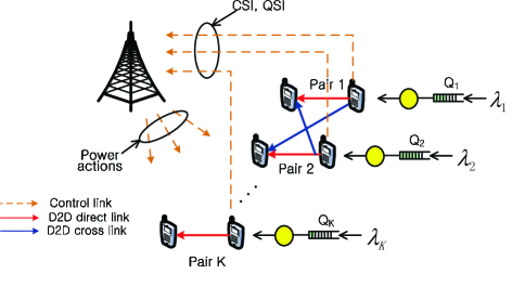
Figure 1: Topology of an infrastructure-assisted D2D communications system.

In this paper, we first establish the PHY, MAC and bursty data source models as well as the queue dynamics in Section II. We formally formulate the associated stochastic optimization problem of the dynamic power control for delay-aware D2D communications as an infinite horizon average cost MDP. To overcome the aforementioned technical challenges, we exploit specific problem structures in D2D communications. Specifically, 1) the CSMA-like MAC protocol is adopted to coordinate the transmissions of the D2D nodes in a distributive way and this induces a weak interference topology among the simultaneously transmitting D2D nodes, and 2) the assistance of the BS substantially simplifies the signaling mechanism of control information exchange. We derive a simplified optimality condition for solving the MDP in Section III. Compared with the conventional Bellman equation [12], the derived optimality condition involves solving a $K$-dimensional partial differential equation (PDE) only. Utilizing the interference filtering property of the MAC protocol, we obtain a closed-form approximate priority function and the associated error bound using perturbation analysis. Based on that, we obtain a delay-aware low complexity dynamic power control algorithm for the D2D communications in Section IV. The solution is shown to be asymptotically optimal for a sufficiently large carrier sensing distance in the MAC protocol. Furthermore, in Section V, we show that the proposed solution achieves significant performance gain over various baseline schemes.

II System Model

In this section, we introduce the system model for the infrastructure-assisted D2D communications, including the D2D system topology, the physical layer model, the MAC layer model and the bursty data source model. We first list the important notations in this paper in Table 1.

TABLE I: List of important notations

Symbol		Meaning
$K$		number of D2D pairs
$\mathbf{P}=\{P_{k}\}$		transmit power
$\mathbf{H}=\{H_{kj}\}$		global CSI
$\mathbf{L}=\{L_{kj}\}$		large-scale path gain
$\boldsymbol{\sigma}=\{\sigma_{k}\}$		MAC output
$\boldsymbol{\nu}=\{\nu_{k}\}$		probability of accessing the channel
$\mathbf{A}=\{A_{k}\}$		bit/packet arrival
$\boldsymbol{\lambda}=\{\lambda_{k}\}$		average arrival rate
$\mathbf{Q}=\{Q_{k}\}$		global QSI
$\boldsymbol{\chi}=\{\boldsymbol{\sigma},\mathbf{H},\mathbf{Q}\}$		global system state
$\boldsymbol{\Omega}(\boldsymbol{\chi})=\{\Omega_{k}(\boldsymbol{\chi})\}$		power control policy
$\tau$		duration of a time slot
$C_{k}(\mathbf{H},\mathbf{P})$		achievable data rate of the $k$-th D2D pair
$\delta$		carrier sensing distance
$L^{\delta}$		worst-case cross-channel path gain
$V^{*}(\mathbf{Q})$		priority function

II-A D2D System Topology

We consider an infrastructure-assisted D2D communications system, as shown in Fig. 1. Specifically, the D2D system consists of two tiers, namely the cellular tier and the D2D tier. In the D2D tier, there are $K$ transmitter-receiver (Tx-Rx) pairs located randomly in the area of a cell. Transmitter $k$ transmits data to receiver $k$, and the Tx-Rx pair is associated by the D2D peer discovery procedure [2]. All D2D pairs share a common channel, which is orthogonal to the channels used in the cellular tier. Hence, there is no cross-tier interference between the cellular and D2D tiers. In the cellular tier, the BS plays the role of the centralized controller for the D2D communications. Each D2D pair communicates directly on a single-hop link in a distributed ad-hoc manner with the assistance of the cellular BS. The time is slotted, and the duration of each time slot is $\tau$. The cellular BS collects necessary information and broadcasts the resource allocation actions (calculated based on the collected information) periodically to the D2D nodes at the beginning of each time slot.

II-B Physical Layer Model

Let $s_{k}$ denote the information symbol for the $k$-th D2D pair. The received signal at receiver $k$ is

$$y_{k}=\underbrace{h_{kk}\sqrt{P_{k}}s_{k}}_{\text{desired signal}}+\underbrace{\sum_{j\neq k}h_{kj}\sqrt{P_{j}}s_{j}}_{\text{interference}}+\underbrace{z_{k}}_{\text{noise}}$$ (1)

where $h_{kj}$ is the complex channel fading coefficient between transmitter $j$ and receiver $k$, and $z_{k}\sim\mathcal{CN}(0,N_{0})$ is the i.i.d. complex Gaussian channel noise with power $N_{0}$. $P_{k}$ is the transmitter power for $s_{k}$. Let $\mathbf{H}(t)=\{H_{kj}(t):\forall j,k\}$ be the global CSI, where $H_{kj}(t)=|h_{kj}(t)|^{2}$ is the instantaneous channel path gain from transmitter $j$ to receiver $k$ at the $t$-th time slot. We consider the CSI according to the block fading channel model [18, 19] and have the following assumption on $\mathbf{H}$:

Assumption 1 (Short-Term CSI Model)

The CSI $\mathbf{H}(t)$ remains constant within a time slot and is i.i.d. over time slots. $H_{kj}(t)$ follows a negative exponential distribution with mean $L_{kj}$. Furthermore, $H_{kj}(t)$ is independent w.r.t. the D2D pair indices $k,j$.  ∎

Note that $L_{kj}$ is the large-scale path gain from transmitter $j$ to receiver $k$. Let $\mathbf{L}=\{L_{kj}:\forall j,k\}$, and we have the following assumption on $\mathbf{L}$.

Assumption 2 (Long-Term Path Gain Model)

The long-term large-scale path gain $\mathbf{L}$ is constant for the duration of the communication session. Specifically, for any transmitter $j$ and receiver $k$, the relationship between the path gain $L_{kj}$ and the distance $d_{kj}$ is $L_{kj}=\frac{G_{k}^{r}G_{j}^{t}\lambda^{2}}{\left(4\pi d_{kj}\right)^{2}}$ ($\forall k,j$), where $G_{k}^{r}$ and $G_{j}^{t}$ are the receive and transmit antenna gains respectively, and $\lambda$ is the carrier wavelength.  ∎

Let $\mathbf{P}(t)=\{P_{k}(t):\forall k\}$ be the collection of the transmit power of all the D2D transmitters at the $t$-th time slot. For given CSI $\mathbf{H}(t)$ and power actions $\mathbf{P}(t)$, the achievable data rate of the $k$-th Tx-Rx pair depends on the SINR by treating interference as noise, which is calculated as

$$C_{k}(\mathbf{H}(t),\mathbf{P}(t))=\log_{2}\left(1+{\frac{1}{\Gamma}}\frac{H_{kk}(t)P_{k}(t)}{N_{0}+\sum_{j\neq k}H_{kj}(t)P_{j}(t)}\right)$$ (2)

where $\Gamma$ is the SINR gap [21] to measure the practical reduction of the SINR with respect to the capacity. $\Gamma$ depends on the error probability requirement as well as the modulation scheme.

II-C MAC Layer Model

The D2D nodes utilize a CSMA-like protocol to arbitrate the random channel access in a distributed manner. The basic principle of the CSMA is listen-before-talk [22], which is used to avoid collision between simultaneous transmissions of neighboring nodes. As a result, the MAC protocol determines the subset of the D2D nodes in which the transmitters can transmit data simultaneously without causing excessive interference. For simplicity, we consider the following idealized MAC protocol model, which has been widely adopted in justifying the hardcore point process [23].

Assumption 3 (Hardcore Point Process Model)

The D2D nodes adopt a CSMA-like MAC protocol with the carrier sensing distance $\delta$. The output of the MAC protocol is captured by the MAC output process $\boldsymbol{\sigma}(t)=(\sigma_{1}(t),\cdots,\sigma_{K}(t))\in\{0,1\}^{K}$, where $\sigma_{k}(t)=1$ means that the $k$-th D2D node accesses the channel at the $t$-th time slot. The MAC output process $\boldsymbol{\sigma}(t)$ has the following properties:

• ${\sigma}_{k}(t)$ is i.i.d. over time slots according to the Bernoulli distribution with mean $\mathbb{E}[\sigma_{k}(t)]=\nu_{k}\left(\delta\right)$.

• all transmit nodes have equal opportunity to access the channel, i.e., $\nu_{k}\left(\delta\right)=\frac{1}{\left|\mathcal{N}_{k}\left(\delta\right)\right|+1}$, where $\mathcal{N}_{k}\left(\delta\right)$ is the set of transmit nodes within the carrier sensing distance $\delta$ from transmitter $k$ and $\left|\mathcal{N}_{k}\left(\delta\right)\right|$ is the associated cardinality.

• during each time slot $t$, a feasible $\boldsymbol{\sigma}(t)$ satisfies the following carrier sensing constraint: if $\sigma_{k}(t)=1$, then $\sigma_{j}(t)=0$ for all $j\in\mathcal{N}_{k}$. ∎

The first condition corresponds to the memoryless property of the MAC protocol with respect to the channel access. The second condition corresponds to the fairness among the D2D nodes in the neighbour set, and the third condition corresponds to the carrier sensing requirement in the MAC protocol. Note that $\nu_{k}(\delta)$ corresponds to the spatial reuse factor for transmitter $k$ in the D2D network for a given carrier sensing distance $\delta$. Furthermore, $\nu_{k}\left(\delta\right)$ and $\mathcal{N}_{k}\left(\delta\right)$ depend on the topology of the D2D nodes.

II-D Bursty Data Source and Queue Dynamics

There is a bursty data source at each D2D transmitter. Let $\mathbf{A}(t)=(A_{1}(t)\tau,\cdots,A_{K}(t)\tau)$ be the random arrivals (number of bits) from the application layers to the $K$ D2D transmitters at the end of the $t$-th time slot. We have the following assumption on $\mathbf{A}(t)$.

Assumption 4 (Bursty Source Model)

Assume that $A_{k}\left(t\right)$ is i.i.d. over decision slots according to a general distribution $\Pr[A_{k}]$. The moment generating function of $A_{k}$ exists with $\mathbb{E}[A_{k}]=\lambda_{k}$. $A_{k}\left(t\right)$ is independent w.r.t. $k$. Furthermore, the arrival rates $(\lambda_{1},\dots,\lambda_{K})$ lie within the stability region [24] of the system.  ∎

Each D2D transmitter has a data queue for the bursty traffic flows towards the associated receiver. Let $Q_{k}(t)\in[0,\infty)$ be the queue length (number of bits) at transmitter $k$ at the beginning of the $t$-th slot. Let $\mathbf{Q}(t)=(Q_{1}(t),\cdots,Q_{K}(t))\in\boldsymbol{\mathcal{Q}}\triangleq[0,\infty)^{K}$ be the global QSI. The queue dynamics of transmitter $k$ is

$$Q_{k}(t+1)=\max\left\{Q_{k}(t)-\sigma_{k}(t)C_{k}(\mathbf{H}(t),\mathbf{P}(t))\tau,0\right\}+A_{k}(t)\tau$$ (3)

Remark 1 (Weak Coupling Property of Queue Dynamics)

The $K$ queue dynamics in the D2D system are coupled together due to the interference term in (2). Specifically, the departure of the queue at each transmitter depends on the power actions of all the $K$ D2D transmitters. Furthermore, the CSMA-like mechanism in the MAC protocol model in Assumption 3 contributes to filtering the strong interference between the active D2D transmitters. Let $L^{\delta}=\max\{L_{kj}:\forall k\neq j,d_{kj}>\delta\}$ be the worst-case cross-channel path gain for a given sensing threshold $\delta$. Due to the interference filtering property of the MAC protocol, there is only weak queue coupling in the D2D network, and $L^{\delta}$ measures the coupling intensity. We will leverage this weak coupling property to derive low complexity closed-form approximate solutions in Section IV. ∎

III Delay-Aware Cross-Layer Control Framework

In this section, we formally formulate the delay-aware cross-layer radio resource control framework for D2D communications. We first define the control policy and the optimization objective. We then formulate the design as a Markov Decision Process (MDP) and derive the optimality conditions for solving the problem.

III-A Power Control Policy

For delay-sensitive applications, it is important to dynamically adapt the transmit power of the D2D nodes based on the instantaneous realizations of the CSI (captures the instantaneous transmission opportunities) and the QSI (captures the urgency of the $K$ data flows). Let $\boldsymbol{\chi}=(\boldsymbol{\sigma},\mathbf{H},\mathbf{Q})$ denote the global system state. We define the stationary power control policy below.

Definition 1 (Stationary Power Control Policy)

A stationary control policy for the $k$-th D2D transmitter $\Omega_{k}$ is a mapping from the system state $\boldsymbol{\chi}$ to the power control action of transmitter $k$. Specifically, $\Omega_{k}(\boldsymbol{\chi})=P_{k}\geq 0$. Let $\boldsymbol{\Omega}=\{\Omega_{k}:\forall k\}$ denote the aggregation of the control policies for all the $K$ D2D transmitters. ∎

Since the D2D nodes access the channel randomly, the MAC output $\boldsymbol{\sigma}$ is i.i.d. over time slots. The CSI $\mathbf{H}$ is i.i.d. over time slots based on the block fading channel model in Assumption 1. Furthermore, from the queue evolution equation in (3), $\mathbf{Q}(t+1)$ depends only on $\mathbf{Q}(t)$ and the data rate. Given a control policy $\boldsymbol{\Omega}$, the data rate at the $t$-th time slot depends on $\sigma_{k}(t)$, $\mathbf{H}(t)$ and $\boldsymbol{\Omega}(\boldsymbol{\chi(t)})$. Hence, the global system state ${\boldsymbol{\chi}(t)}$ is a controlled Markov chain [12] with the transition probability

$$\Pr[\boldsymbol{\chi}(t+1)|\boldsymbol{\chi}(t),\boldsymbol{\Omega}(\boldsymbol{\chi}(t))]$$ (4)

$$= \Pr[\boldsymbol{\sigma}(t+1)]\Pr[\mathbf{H}(t+1)]\Pr[\mathbf{Q}(t+1)|\boldsymbol{\chi}(t),\boldsymbol{\Omega}(\boldsymbol{\chi}(t))]$$

where the queue transition probability is given by

$$\Pr[\mathbf{Q}(t+1)|\boldsymbol{\chi}(t),\boldsymbol{\Omega}(\boldsymbol{\chi}(t))]$$

$$= \left\{\begin{aligned} &\prod_{k}\Pr\big{[}A_{k}\left(t\right)\big{]},\ \ {\color[rgb]{0,0,0}\text{if }Q_{k}\left(t+1\right)\text{is given by (\ref{queueing})},\forall k}\\ &\ 0,\hskip 73.97733pt\text{otherwise}\end{aligned}\right.$$ (5)

For technical reasons, we consider the admissible control policy defined below.

Definition 2 (Admissible Control Policy)

A policy $\boldsymbol{\Omega}$ is admissible if the following requirements are satisfied:

• $\boldsymbol{\Omega}$ is a unichain policy, i.e., the controlled Markov chain $\left\{\boldsymbol{\chi}\left(t\right)\right\}$ under $\boldsymbol{\Omega}$ has a single recurrent class (and possibly some transient states) [12].

• The queueing system under $\boldsymbol{\Omega}$ is third-order stable in the sense that $\lim_{t\rightarrow\infty}\mathbb{E}^{\boldsymbol{\Omega}}[\sum_{k=1}^{K}Q_{k}^{3}(t)]<\infty$, where $\mathbb{E}^{\boldsymbol{\Omega}}$ means taking expectation w.r.t. the probability measure induced by the control policy $\boldsymbol{\Omega}$. ∎

III-B Problem Formulation

As a result, under an admissible control policy $\boldsymbol{\Omega}$, the average delay cost for the $k$-th D2D pair is given by

$$\overline{D}_{k}(\boldsymbol{\Omega})=\limsup_{T\rightarrow\infty}\frac{1}{T}\sum_{t=0}^{T-1}\mathbb{E}^{\boldsymbol{\Omega}}\left[\frac{Q_{k}\left(t\right)}{\lambda_{k}}\right],\quad\forall k$$ (6)

Similarly, under an admissible control policy $\boldsymbol{\Omega}$, the average power cost of the $k$-th D2D transmitter is given by

$$\overline{P}_{k}(\boldsymbol{\Omega})=\limsup_{T\rightarrow\infty}\frac{1}{T}\sum_{t=0}^{T-1}\mathbb{E}^{\boldsymbol{\Omega}}\big{[}P_{k}(t)\big{]},\quad\forall k$$ (7)

We formulate the dynamic power control problem for the delay-aware D2D system as follows:

Problem 1 (Power Control for Delay-Aware D2D Systems)

The power control problem for the delay-aware D2D communications is formulated as

$$\underset{\boldsymbol{\Omega}}{\min}~{}~{}~{} L(\boldsymbol{\Omega})$$ (8)

$$= \sum_{k=1}^{K}\Big{(}\beta_{k}\underbrace{\overline{D}_{k}(\boldsymbol{\Omega})}\limits_{\text{average}\atop\text{delay}}+\gamma_{k}\underbrace{\overline{P}(\boldsymbol{\Omega})}\limits_{\text{average}\atop\text{power}}\Big{)}$$

$$= \limsup_{T\rightarrow\infty}\frac{1}{T}\sum_{t=0}^{T-1}\mathbb{E}^{\boldsymbol{\Omega}}\left[c\left(\mathbf{Q}\left(t\right),\boldsymbol{\Omega}\left(\boldsymbol{\chi}\left(t\right)\right)\right)\right]$$

where $c\left(\mathbf{Q},\mathbf{P}\right)=\sum_{k=1}^{K}\left(\beta_{k}\frac{Q_{k}}{\lambda_{k}}+\gamma_{k}P_{k}\right)$. $\mbox{\boldmath$\beta$}=\{\beta_{k}>0:\forall k\}$ and $\mbox{\boldmath$\gamma$}=\{\gamma_{k}>0:\forall k\}$ are positive weights for the delay cost and the power cost respectively.   ∎

Problem 1 embraces various optimization formulations such as minimizing the average delay subject to the average power constraint or minimizing the average transmit power subject to the average delay constraint. This is because these “constrained optimization problems” have the same Lagrangian function, which is given by (8) in Problem 1. The weights $\boldsymbol{\beta}$ and $\boldsymbol{\gamma}$ are equivalent to the Lagrangian multipliers of the associated constraints. Also note that Problem 1 is an infinite horizon average cost MDP, which is known as a very difficult problem.

III-C Optimality Conditions for Power Control Problem

Problem 1 is an MDP, and the associated Bellman equation [12] involves the entire system state $\boldsymbol{\chi}=(\boldsymbol{\sigma},\mathbf{H},\mathbf{Q})$. Exploiting the i.i.d. properties of $\mathbf{H}(t)$ and $\boldsymbol{\sigma}(t)$, we obtain the following equivalent Bellman equation.

Theorem 1 (Sufficient Conditions for Optimality)

For any given weights $\beta$ and $\gamma$, assume there exists a $(\theta^{*},\{V^{*}(\mathbf{Q})\})$ that solves the following equivalent Bellman equation:

$$\theta^{*}\tau+V^{*}(\mathbf{Q})\hskip 113.81102pt\forall\mathbf{Q}\in\boldsymbol{\mathcal{Q}}$$ (9)

$$= \mathbb{E}\bigg{[}\min_{\boldsymbol{\Omega}(\boldsymbol{\chi})}\Big{[}c\big{(}\mathbf{Q},\boldsymbol{\Omega}\big{(}\boldsymbol{\chi}\big{)}\big{)}\tau+\sum_{\mathbf{Q}^{\prime}}\Pr\big{[}\mathbf{Q}^{\prime}\big{|}\boldsymbol{\chi},\boldsymbol{\Omega}\big{(}\boldsymbol{\chi}\big{)}\big{]}V^{*}(\mathbf{Q}^{\prime})\Big{]}\bigg{|}\mathbf{Q}\bigg{]}$$

Furthermore, for all admissible control policy $\boldsymbol{\Omega}$, $V^{\ast}$ satisfies the following transversality condition:

$$\lim_{T\rightarrow\infty}\frac{1}{T}\mathbb{E}^{\boldsymbol{\Omega}}\left[V^{\ast}\left(\mathbf{Q}\left(T\right)\right)\right]=0$$ (10)

Then ${\theta^{*}}=\underset{\boldsymbol{\Omega}}{\min}L(\boldsymbol{\Omega})$ is the optimal average cost, and $V^{\ast}\left(\mathbf{Q}\right)$ is the priority function of the $K$ data flows. If $\boldsymbol{\Omega}^{\ast}\left(\boldsymbol{\chi}\right)$ attains the minimum of the R.H.S. of (9) for all $\mathbf{Q}\in\boldsymbol{\mathcal{Q}}$, then $\boldsymbol{\Omega}^{*}$ is the optimal control policy for Problem 1. ∎

Proof:

Please refer to Appendix A. ∎

Remark 2 (Interpretation of Theorem 1)

At each stage when the queue length is $\mathbf{Q}(t)$, the optimal action has to strike a balance between the current cost and the future cost because the action taken will affect the future evolution of $\mathbf{Q}(t+1)$. Furthermore, based on the unichain property of the admission control policy, the solution obtained from Theorem 1 is unique [12].  ∎

IV Low-Complexity Power Control Solution

One key obstacle in deriving the optimal power control policy $\boldsymbol{\Omega}^{\ast}$ is to obtain the priority function for the Bellman equation in (9). Conventional brute force value iteration or policy iteration algorithms can only give numerical solutions and have exponential complexity in $K$, which is highly undesirable. In this section, we shall exploit the interference filtering property of the MAC protocol and adopt perturbation theory to obtain a closed-form approximation of the priority function $V^{\ast}(\mathbf{Q})$ and derive the associated error bound. Based on that, we obtain a low complexity dynamic power control algorithm for the delay-aware D2D communications.

IV-A Closed-Form Approximate Priority Function via Perturbation Analysis

We adopt a calculus approach to obtain a closed-form approximate priority function. We first have the following theorem for solving the Bellman equation in (9).

Theorem 2 (Calculus Approach for Solving (9))

Assume there exist $c^{\infty}$ and $J\left(\mathbf{Q};L^{\delta}\right)$ of class $\mathcal{C}^{2}(\mathbb{R}_{+}^{K})$ that satisfy

• the following partial differential equation (PDE):

  $$\mathbb{E}\Bigg{[}\min_{\boldsymbol{\Omega}\left(\boldsymbol{\chi}\right)}\bigg{[}\sum_{k=1}^{K}\left(\beta_{k}\frac{Q_{k}}{\lambda_{k}}+\gamma_{k}P_{k}\right)-c^{\infty}\hskip 22.76228pt\forall\mathbf{Q}\in\mathbb{R}_{+}^{K}$$

  $$+\sum_{k=1}^{K}\bigg{(}\frac{\partial J\left(\mathbf{Q};L^{\delta}\right)}{\partial Q_{k}}\left(\lambda_{k}-\sigma_{k}C_{k}\big{(}\mathbf{H},\mathbf{P}\big{)}\right)\bigg{)}\bigg{]}\Bigg{|}\mathbf{Q}\Bigg{]}=0$$ (11)

  with boundary condition $J\left(\mathbf{0};L^{\delta}\right)=0$.

• $\Big{\{}\frac{\partial J\left(\mathbf{Q};L^{\delta}\right)}{\partial Q_{k}}:\forall k\Big{\}}$ are increasing functions of all $Q_{k}$.

• $J\left(\mathbf{Q};L^{\delta}\right)=\mathcal{O}\left(\|\mathbf{Q}\|^{3}\right)$.

Then, we have

$$\theta^{\ast}=c^{\infty}+o(1),V^{\ast}\left(\mathbf{Q}\right)=J\left(\mathbf{Q};L^{\delta}\right)+o(1),\forall\mathbf{Q}\in\boldsymbol{\mathcal{Q}}$$ (12)

where the error term $o(1)$ asymptotically goes to zero for sufficiently small $\tau$.  ∎

Proof:

please refer to Appendix B. ∎

Theorem 2 suggests that if we can solve for the PDE in (11), then the solution $(J\left(\mathbf{Q};L^{\delta}\right),c^{\infty})$ is only $o(1)$ away from the solution of the Bellman equation $(V^{*}(\mathbf{Q}),\theta^{*})$. Before we solve the $K$-dimensional PDE in (11), we first recognize that due to the interference filtering property of the MAC protocol in Assumption 3, the cross-channel path gain of all the active D2D flows are quite weak and the worst-case interfering path gain is $L^{\delta}$. Note that the solution of (11) depends on the worst-case cross-channel path gain $L^{\delta}$ and, hence, the $K$-dimensional PDE in (11) can be regarded as a perturbation of a base system defined below.

Definition 3 (Base System)

A base system is characterized by the PDE in (11) with $L^{\delta}=0$.  ∎

We then study the base system and use $J(\mathbf{Q};0)$ to obtain a closed-form approximation of $J(\mathbf{Q};L^{\delta})$. We have the following lemma summarizing the priority function $J(\mathbf{Q};0)$ of the base system.

Lemma 1 (Decomposable Structure of $J(\mathbf{Q};0)$)

The solution $J(\mathbf{Q};0)$ for the base system has the following decomposable structure:

$$J\left(\mathbf{Q};0\right)=\sum_{k=1}^{K}J_{k}\left(Q_{k}\right)$$ (13)

where $J_{k}\left(Q_{k}\right)$ is the per-flow priority function for the $k$-th data flow given by

$$\left\{\begin{aligned} Q_{k}(y)=&\frac{\lambda_{k}}{\beta_{k}}\left(\frac{a_{k}}{(|\mathcal{N}_{k}(\delta)|+1)\ln 2}E_{1}\left(\frac{a_{k}}{y}\right)-\lambda_{k}y\right.\\ &\left.-\frac{y}{(|\mathcal{N}_{k}(\delta)|+1)\ln 2}\left(e^{-\frac{a_{k}}{y}}-E_{1}\left(\frac{a_{k}}{y}\right)\right)+c_{k}^{\infty}\right)\\ J_{k}(y)=&\frac{\lambda_{k}}{\beta_{k}}\left(\frac{1}{4(|\mathcal{N}_{k}(\delta)|+1)\ln 2}E_{1}\left(\frac{a_{k}}{y}\right)\left(2y^{2}-a_{k}^{2}\right)\right.\\ &\left.-\frac{y(y-a_{k})}{4(|\mathcal{N}_{k}(\delta)|+1)\ln 2}e^{-\frac{a_{k}}{y}}-\frac{\lambda_{k}y^{2}}{2}\right)+b_{k}\end{aligned}\right.$$ (14)

where $a_{k}\triangleq\frac{N_{0}{\Gamma}\gamma_{k}\ln 2}{L_{kk}}$. $c_{k}^{\infty}=\frac{1}{(|\mathcal{N}_{k}(\delta)|+1)\ln 2}\left(d_{k}e^{-\frac{a_{k}}{d_{k}}}-a_{k}E_{1}\left(\frac{a_{k}}{d_{k}}\right)\right)$, where $d_{k}$ satisfies $\frac{1}{(|\mathcal{N}_{k}(\delta)|+1)\ln 2}E_{1}\left(\frac{a_{k}}{d_{k}}\right)=\lambda_{k}$. $E_{1}(z)\triangleq\int_{1}^{\infty}\frac{e^{-tz}}{t}\mathrm{d}t=\int_{z}^{\infty}\frac{e^{-t}}{t}\mathrm{d}t$. $b_{k}$ is chosen to satisfy the boundary condition $J_{k}(0)=0$.  ∎

Proof:

please refer to Appendix C. ∎

Note that when $L^{\delta}=0$, the interference network has $L_{kj}=0$ for all $k\neq j$ with $d_{kj}>\delta$ and, hence, there is no interference between the active D2D ndoes. As a result, the $K$ D2D flows are totally decoupled and the system is equivalent to a decoupled system with $K$ independent D2D flows. That is why the priority function $J\left(\mathbf{Q};0\right)$ in the base system has the decomposable structure in Lemma 1.

We then analyze the asymptotic property of the per-flow priority function $J_{k}\left(Q_{k}\right)$ in Corollary 1.

Corollary 1 (Asymptotic Property of $J_{k}\left(Q_{k}\right)$)

$$J_{k}\left(Q_{k}\right) =\frac{\beta_{k}(|\mathcal{N}_{k}(\delta)|+1)}{2\lambda_{k}}\frac{Q_{k}^{2}}{\log_{2}\left(Q_{k}\right)}+o\left(\frac{Q_{k}^{2}}{\log_{2}\left(Q_{k}\right)}\right),$$

$$\hskip 142.26378pt\text{as }Q_{k}\rightarrow\infty$$ (15)

Proof:

Please refer to Appendix D. ∎

Next, we study the PDE in (11) for large $\delta$. Note that large $\delta$ corresponds to small cross-channel path gains within the set of active D2D nodes. Hence, $J(\mathbf{Q};L^{\delta})$ can be considered as a perturbation of the solution of the base system $J(\mathbf{Q};0)$. Using perturbation analysis, we establish the following theorem on the approximation of $J(\mathbf{Q};L^{\delta})$:

Theorem 3 (First Order Approximation of $J\left(\mathbf{Q};L^{\delta}\right)$)

$J\left(\mathbf{Q};L^{\delta}\right)$ can be approximated by $J\left(\mathbf{Q};0\right)$, and the first order perturbation term is given by

$$J\left(\mathbf{Q};L^{\delta}\right)= J\left(\mathbf{Q};0\right)+\sum_{k=1}^{K}\sum_{j\neq k\atop j\notin\mathcal{N}_{k}(\delta)}\Big{(}\frac{D_{kj}L_{kj}Q_{k}^{2}Q_{j}}{(\log_{2}Q_{k})^{2}\log_{2}Q_{j}}$$

$$+o\left(\frac{D_{kj}L_{kj}Q_{k}^{2}Q_{j}}{(\log_{2}Q_{k})^{2}\log_{2}Q_{j}}\right)\Big{)}+\mathcal{O}\left(\frac{1}{\delta^{4}}\right)$$ (16)

where $D_{kj}=\frac{\beta_{k}\beta_{j}(|\mathcal{N}_{k}(\delta)|+1)}{2(\ln 2)\lambda_{k}\lambda_{j}\gamma_{j}N_{0}}$.  ∎

Proof:

Please refer to Appendix E. ∎

The priority function $V(\mathbf{Q})$ is decomposed into the following three terms: 1) the base term $\sum_{k}J_{k}(Q_{k})$ obtained by solving a base system without coupling, 2) the perturbation term accounting for the first order interference coupling due to simultaneously transmitting D2D nodes after MAC filtering, and 3) the residual error term. As a result, we adopt the following closed-form approximation of $V(\mathbf{Q})$:

$$\widetilde{V}\left(\mathbf{Q}\right)\triangleq\sum_{k=1}^{K}J_{k}\left(Q_{k}\right)+\sum_{k=1}^{K}\sum_{j\neq k\atop j\notin\mathcal{N}_{k}(\delta)}\frac{D_{kj}L_{kj}Q_{k}^{2}Q_{j}}{(\log_{2}Q_{k})^{2}\log_{2}Q_{j}}$$ (17)

Remark 3 (Approximation Error w.r.t. System Parameters)

• Approximation Error w.r.t. Traffic Loading: the approximation error is a decreasing function of the average arrival rate $\lambda_{k}$.

• Approximation Error w.r.t. SNR: the approximation error is an increasing function of the SNR (which is a decreasing function of $\gamma_{k}$).

• Approximation Error w.r.t. Sensing Distance: the approximation error is a decreasing function of the carrier sensing distance at the order at least $\mathcal{O}\left(\frac{1}{\delta^{2}}\right)$.

From Corollary 1 and (17), the priority function $\widetilde{V}(\mathbf{Q})=\mathcal{O}(\frac{Q_{k}^{2}}{\log Q_{k}})$ for large $Q_{k},\forall k$. As a result, the longer queue will get higher priority in the order of $\frac{Q_{k}}{\log Q_{k}}$. Based on Theorem 1 and Theorem 3, the approximation error between the optimal priority function $V^{\ast}\left(\mathbf{Q}\right)$ in Theorem 1 and the closed-form approximate priority function $\widetilde{V}\left(\mathbf{Q}\right)$ in (17) is $\mathcal{O}(\frac{1}{\delta^{2}})+o(1)$. In other words, the error terms are asymptotically small w.r.t. the carrier sensing distance $\delta$ and the slot duration.

IV-B Asymptotically Delay-Optimal Power Control Algorithm

In this section, we use the closed-form approximate priority function in (17) to capture the urgency information of the $K$ D2D pairs and obtain low complexity delay-aware power control. Using the approximate priority function in (17) and Lemma 2, the per-stage control problem (for each state realization $\boldsymbol{\chi}$) is given by

$$\max_{\mathbf{P}}\ \sum_{k=1}^{K}\Big{(}\underbrace{\frac{\partial\widetilde{V}\left(\mathbf{Q}\right)}{\partial Q_{k}}}_{\text{flow weight}}\sigma_{k}\underbrace{C_{k}\left(\mathbf{H},\mathbf{P}\right)}_{\text{data rate}}-\gamma_{k}P_{k}\Big{)}$$ (18)

where $\frac{\partial\widetilde{V}\left(\mathbf{Q}\right)}{\partial Q_{k}}$ can be calculated from (17) which is given by

$$\frac{\partial\widetilde{V}\left(\mathbf{Q}\right)}{\partial Q_{k}}=J_{k}^{\prime}\left(Q_{k}\right)$$ (19)

$$+\sum_{j\neq k\atop j\notin\mathcal{N}_{k}(\delta)}\frac{Q_{j}(\ln Q_{k}-1)}{(\ln 2)\log_{2}^{2}Q_{k}\log_{2}Q_{j}}\left(\frac{2D_{kj}L_{kj}Q_{k}}{\log_{2}Q_{k}}+\frac{D_{jk}L_{jk}Q_{j}}{\log_{2}Q_{j}}\right)$$

The per-stage problem in (18) is similar to the weighted sum-rate (WSR) optimization subject to the power constraint, which has been widely studied in [25] and [26]. However, unlike conventional WSR problems where the weights are static, the weights here in (18) are dynamic and are determined by the QSI via the priority function $\frac{\partial\widetilde{V}(\mathbf{Q})}{\partial Q_{k}}$. As such, the role of the QSI is to dynamically adjust the weight (priority) of the individual flows, whereas the role of the CSI is to adjust the priority of the flow based on the transmission opportunity in the rate function $C_{k}(\mathbf{H},\mathbf{P})$. Note that the per-stage problem in (18) is challenging due to the non-convexity of $C_{k}\left(\mathbf{H},\mathbf{P}\right)$ w.r.t. $\mathbf{P}$. We shall first derive a low complexity iterative solution that converges to the stationary point of (18). We then show that the converged solution is asymptotically optimal for sufficiently small $L^{\delta}$.

Algorithm 1 (Delay-Aware Dynamic Power Control)

• Step 1 [Initialization]: Let $n=0$. Initialize a feasible $\mathbf{P}(0)$.

• Step 2 [Iteration]: In the $(n+1)$-th iteration, the transmit power of each D2D transmitter is updated based on the power results of the $n$-th iteration according to

  $$P_{k}(n+1)=\left(\frac{\partial\widetilde{V}\left(\mathbf{Q}\right)}{\partial Q_{k}}\frac{1}{(\ln 2)(\gamma_{k}+\zeta_{k}(n))}-\frac{{\Gamma}I_{k}(n)}{{H}_{kk}}\right)^{+}$$ (20)

  where $I_{k}(n)=N_{0}+\sum_{j\neq k,j\notin\mathcal{N}_{k}(\delta)}{H}_{kj}P_{j}(n)$ and $\zeta_{k}(n)=\sum_{j\neq k,j\notin\mathcal{N}_{k}(\delta)}\frac{1}{\ln 2}\frac{\partial\widetilde{V}\left({Q}\right)}{\partial Q_{j}}\frac{{H}_{jj}P_{j}(n){H}_{kj}}{I_{j}(n)(I_{j}(n)+{H}_{jj}P_{j}(n))}$.

• Step 3 [Termination]: Set $n=n+1$ and go to Step 2 until a certain termination condition is satisfied.  ∎

Although the problem in (18) is non-convex in general, we show below that Algorithm 1 converges to the global optimal solution asymptotically for sufficiently large $\delta$.

Corollary 2 (Asymptotic Optimality of Algorithm 1)

Algorithm 1 converges to the unique global optimal point of the problem in (18) for sufficiently large $\delta$.  ∎

Proof:

Please refer to Appendix F. ∎

IV-C Summary of the Overall Solution and Implementation Considerations

We give a summary of the overall dynamic power control solution and discuss some implementation considerations (computational complexity) in the context of LTE-Advanced systems [1]. Specifically, we consider the scenario of fully controlled D2D communications [28] in LTE-Advanced in which the eNodeB takes control of the radio resource for the D2D nodes inside its coverage. A frame is divided into a contention phase, a reporting phase, a decision phase and a data transmission phase, which are described as follows:

1. Contention Phase: D2D nodes access the channels distributively according to a CSMA-like MAC protocol. At the end of the contention phase, each D2D transmitter gets its corresponding MAC output $\sigma_{k}(t)$. Also, during this phase, the CSI $\mathbf{H}(t)$ could be estimated by the D2D receivers.

2. Reporting Phase: Each of the active transmitters ($\mathcal{A}(t)=\{k:\sigma_{k}(t)=1\}$) report their local CSI $\{H_{kj}(t):\forall j\}$ and local QSI $Q_{k}(t)$ to the eNodeB via Physical Uplink Control Channel (PUCCH) and Physical Uplink Shared Channel (PUSCH) [29], respectively.

3. Decision Phase: After receiving the CSI and QSI reports, the eNodeB calculates the optimal power for the active D2D nodes according to the proposed Algorithm 1, and broadcasts the power control actions to the active D2D nodes via Physical Downlink Control Channel (PDCCH) [29].

4. Data Transfer Phase: The active D2D transmitters adjust their transmit power according to the power control broadcasted from the eNodeB and transmit data during the data transmission phase in the current frame.

Remark 4 (Computational Complexity Consideration)

The computational complexity of the proposed solution is very low. Specifically, most of complexity comes from computing the priority function in (17) and computing the power control actions using Algorithm 1. The complexity of computing the priority function is very low (due to the closed form characterization) compared with conventional brute-force value iterations algorithms [12], which have exponential complexity in $K$. Computing the power control actions using Algorithm 1 is similar to those conventional iterative water-filling solutions for solving WSR optimization in [25]. We shall quantify the complexity comparison in Section V.  ∎

Remark 5 (Extension for OFDMA and General Fading)

The solution framework in Theorem 2 and Theorem 3 can be extended easily to multi-channel systems (such as OFDMA [30]) as well as general fading distributions. For OFDMA systems, the modification required is the rate equation in (2). Each channel can be treated independently since orthogonal parallel channels do not introduce additional coupling. For general fading distributions, the modification required is the solution of the per-flow PDE in the base system $J_{k}\left(Q_{k}\right)$ in Lemma 1.   ∎

V Simulation Results

In this section, we evaluate the performance of the proposed low-complexity power control scheme for D2D communications. The following four baseline schemes are adopted for performance comparison.

• Baseline 1 [Cellular Mode]: The Tx-Rx pairs transmit their data via the cellular BS in a conventional way [5]. The $K$ pairs share the channel using TDMA in a Round-Robin way.

• Baseline 2 [D2D with Fixed Power]: The transmitters always transmit with the maximum power for D2D communications [5].

• Baseline 3 [D2D with CSI-based Power Control]: Large deviation [31] is an approach to bypass the complex delay minimization by converting the delay constraint into an equivalent rate constraint. The CSI-based power control scheme determines the transmit power for maximizing the total data rate without considering the queueing information [32].

• Baseline 4 [D2D with Queue-weighted Power Control]: Lyapunov drift approach [24] considers queue stabilization instead of delay minimization. The queue-weighted power control scheme exploits both CSI and QSI, and solves the per-stage problem (18) replacing $\frac{\partial\widetilde{V}(\mathbf{Q})}{\partial Q_{k}}$ with $Q_{k}$. It is similar to the Modified Largest Weighted Delay First algorithm in [33] but with a modified objective function.

In the simulations, 10 D2D pairs are considered in a single cell with radius 500m. The transmitters are located randomly in the cell and the receivers appear within the D2D communication range of their corresponding transmitters, which is set to 50m. The carrier sensing distance $\delta$ is 100m. Poisson data arrival is considered with a uniform distributed average arrival rate, which has mean 5Mbps. The path gain is calculated as $L_{kj}=15.3+37.6\log_{10}d_{kj}$ [34] with the fading coefficient distributed as $\mathcal{CN}(0,1)$. The average transmit power is 23dBm and the noise power spectrum density is -174dBm/Hz. The system bandwidth is 10MHz. The duration of the time slot is 1ms. The SINR gap $\Gamma$ is set to 1 in the simulation. The weights $\gamma_{k}$ are the same and $\beta_{k}=1$ for all $k$. For comparison, the delay performances of different schemes are evaluated with the same average transmit power by adjusting $\gamma_{k}$. For obtaining the average performance, we consider 100 random topologies, each of which has 1000 time slots.

Fig. 2 shows the average delay versus the average arrival rate. For large traffic load, the transmission via D2D communication has significant performance gain compared with the conventional cellular transmission. This is mainly because of the short distance between D2D transmitters and receivers and their efficient spatial reuse. It can also be observed that the proposed power control algorithm outperforms all the baselines, which verifies the accuracy of the priority function approximation in the proposed power control scheme. It is noticed that the delay of the proposed scheme with small arrival rate is not 0 but a small value, because the transmitters could not transmit data in all time slots.

Fig. 3 shows the average delay versus the average transmit power. The proposed power control scheme also achieves better performance than other baseline schemes. A larger transmit power could increase the received power of the desired signal, but, meanwhile, would cause more serious interference to other D2D pairs. Because of the two-fold effect of the transmit power, the change of the average delay performance is relatively small with adjustment of the average transmit power.

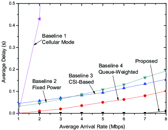
Figure 2: Performance comparison with different average arrival rates

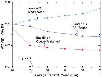
Figure 3: Performance comparison with different average transmit power

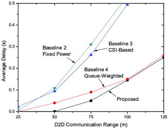
Figure 4: Performance comparison with different D2D communication ranges

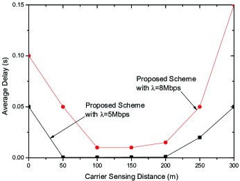
Figure 5: Effect of carrier sensing distance

Fig. 4 indicates the average delay versus the D2D communication range. Unlike the average transmit power, the D2D communication range affects the received power of the desired signal without increasing the interference directly, so the average delay changes a lot with different D2D communication ranges. It can be found that the proposed power control scheme outperforms the baselines when the D2D communication range is small. For large D2D communication ranges (i.e., 100m and 125m), all schemes achieve quite poor delay performance. Note that since the carrier sensing distance $\delta$ is set to 100m here, MAC could not filter the large interference well. Thus, the performance of the proposed power scheme degrades because the weak coupling property of the queue dynamics does not hold when the D2D communication range is too large compared to the carrier sensing distance.

Fig. 5 shows the effect of carrier sensing distance $\delta$ of the proposed power control scheme. As discussed before, a very small sensing distance cannot filter the large interference or guarantee the weak coupling property of the queue dynamics. However, a very large sensing distance leads to inefficient spatial reuse. An appropriate carrier sensing distance should be selected to balance the tradeoff between the above two aspects. From Fig. 5, we observe that the proposed scheme could achieve good delay performance with a large regime of carrier sensing distance.

Table II illustrates the comparison of the MATLAB computational time of the proposed solution, the baselines and the brute-force value iteration algorithm [12] in one time slot. Note that the computation time of Baseline 2 is the smallest in all different $K$ scenarios but it has the worst performance. In addition, the computational time of our proposed scheme is close to those of Baselines 3 & 4 and the difference is due to the computation of the approximate priority function. Therefore, our proposed scheme achieves significant performance gain compared to all the baselines, with small computational complexity cost.

TABLE II: Comparison of the MATLAB computational time

	${\color[rgb]{0,0,0}K=5}$	${\color[rgb]{0,0,0}K=10}$	${\color[rgb]{0,0,0}K=15}$
Baseline 2	$<1$ms	$<1$ms	$<1$ms
Baseline 3 & 4	0.007s	0.015s	0.029s
Proposed Scheme	0.046s	0.091s	0.143s
Brute-Force Value Iteration	$>10^{5}$s	$>10^{5}$s	$>10^{5}$s

VI Conclusion

In this paper, we consider the dynamic power control for delay-aware D2D communications by formulating the associated stochastic optimization problem as an infinite horizon average cost MDP. To deal with the curse of dimensionality, a closed-form approximate priority function is derived using perturbation analysis. Both the analysis and the numerical results show that the approximation error is small and will vanish if the cross-channel path gain goes to 0. Based on the closed-form approximation, we propose a low complexity iterative power control algorithm and discuss some implementation issues for practical systems. Finally, simulation results show that the proposed power control algorithm has significant performance gains in delay performance compared with various state-of-the-art baselines.

Appendix A: Proof of Theorem 1

Following Prop. 4.6.1 of [12], the sufficient conditions for the optimality of Problem 1 are that assume ($\theta^{\ast},\{V^{\ast}\left(\mathbf{Q}\right)\}$) solves the following Bellman equation:

$$\theta^{\ast}{\tau}+V^{\ast}\left(\boldsymbol{\chi}\right)$$

$$= \min_{\boldsymbol{\Omega}(\boldsymbol{\chi})}\Big{[}c\big{(}\mathbf{Q},\boldsymbol{\Omega}\big{(}\boldsymbol{\chi}\big{)}\big{)}{\tau}+\sum_{\boldsymbol{\chi}^{\prime}}\Pr\big{[}\boldsymbol{\chi}^{\prime}\big{|}\boldsymbol{\chi},\boldsymbol{\Omega}\big{(}\boldsymbol{\chi}\big{)}\big{]}V^{\ast}\left(\boldsymbol{\chi}^{\prime}\right)\Big{]}$$

$$= \min_{\boldsymbol{\Omega}(\boldsymbol{\chi})}\Big{[}c\big{(}\mathbf{Q},\boldsymbol{\Omega}\big{(}\boldsymbol{\chi}\big{)}\big{)}{\tau}+\sum_{\mathbf{Q}^{\prime}}\sum_{\mathbf{H}^{\prime}}\sum_{\boldsymbol{\sigma}^{\prime}}\Pr\big{[}\mathbf{Q}^{\prime}\big{|}\boldsymbol{\chi},\boldsymbol{\Omega}\big{(}\boldsymbol{\chi}\big{)}\big{]}$$

$$\hskip 99.58464pt\Pr\big{[}\mathbf{H}^{\prime}\big{]}\Pr\big{[}\boldsymbol{\sigma}^{\prime}\big{]}V^{\ast}\left(\boldsymbol{\chi}^{\prime}\right)\Big{]}$$ (21)

and $V^{\ast}$ satisfies the condition in (10) for all admissible policies $\boldsymbol{\Omega}$. Then ${\theta^{*}}=\underset{\boldsymbol{\Omega}}{\min}L(\boldsymbol{\Omega})$. Taking expectation w.r.t. $\mathbf{H}$ and $\boldsymbol{\sigma}$ on both sizes of (Appendix A: Proof of Theorem 1) and denoting $V^{\ast}\left(\mathbf{Q}\right)=\mathbb{E}\big{[}V^{\ast}\left(\boldsymbol{\chi}\right)\big{|}\mathbf{Q}\big{]}$, we obtain the equivalent Bellman equation in (10) in Theorem 1.

Appendix B: Proof of Theorem 2

In the proof, we shall first establish the relationship between the equivalent Bellman equation in (9) in Theorem 2 and the approximate Bellman equation in (22) in the following Lemma 2. Then, we establish the relationship between the approximate Bellman equation in (22) in the Lemma 2 and the PDE in (11) in Theorem 2.

1. Relationship between the Equivalent Bellman and the Approximate Bellman Equation: We establish the following lemma on the approximate Bellman equation to simplify the equivalent Bellman equation in (9):

Lemma 2 (Approximate Bellman Equation)

For any given weights $\boldsymbol{\beta}$ and $\boldsymbol{\gamma}$, if

• there is a unique ($\theta^{\ast},\{V^{\ast}\left(\mathbf{Q}\right)\}$) that satisfies the Bellman equation and transversality condition in Theorem 1.

• there exist $\theta$ and $V\left(\mathbf{Q}\right)$ of class $\mathcal{C}^{2}(\mathbb{R}_{+}^{K})$ that solve the following approximate Bellman equation:

  $$\theta=\mathbb{E}\bigg{[}\min_{\boldsymbol{\Omega}\left(\boldsymbol{\chi}\right)}\Big{[}c\big{(}\mathbf{Q},\boldsymbol{\Omega}\big{(}\boldsymbol{\chi}\big{)}\big{)}\hskip 28.45274pt\forall\mathbf{Q}\in\boldsymbol{\mathcal{Q}}$$ (22)

  $$\hskip 28.45274pt+\sum_{k=1}^{K}\frac{\partial V\left(\mathbf{Q}\right)}{\partial Q_{k}}\Big{[}\lambda_{k}-\sigma_{k}C_{k}\big{(}\mathbf{H},\Omega(\boldsymbol{\chi})\big{)}\Big{]}\Big{]}\bigg{|}\mathbf{Q}\bigg{]}$$

  and for all admissible control policy $\Omega$, the transversality condition in (10) is satisfied for $V$,

then, we have

$$\theta^{\ast}=\theta+o(1),\quad V^{\ast}\left(\mathbf{Q}\right)=V\left(\mathbf{Q}\right)+o(1),\quad\forall\mathbf{Q}\in\boldsymbol{\mathcal{Q}}$$ (23)

where the error term $o(1)$ asymptotically goes to zero for sufficiently small slot duration $\tau$.  ∎

Proof:

Let $\mathbf{Q}^{\prime}=(Q_{1}^{\prime},\cdots,Q_{k}^{\prime})=\mathbf{Q}(t+1)$ and $\mathbf{Q}=(Q_{1},\cdots,Q_{k})=\mathbf{Q}(t)$. For the queue dynamics in (3) and sufficiently small $\tau$, we have $Q_{k}^{\prime}=Q_{k}-\sigma_{k}C_{k}\left(\mathbf{H},\mathbf{P}\right)+A_{k}\tau$, ($\forall k$). Therefore, if $V\left(\mathbf{Q}\right)$ is of class $\mathcal{C}^{2}(\mathbb{R}_{+}^{K})$, we have the following Taylor expansion on $V\left(\mathbf{Q}^{\prime}\right)$:

$$\mathbb{E}\left[V\left(\mathbf{Q}^{\prime}\right)\big{|}\mathbf{Q}\right]$$ (24)

$$= V\left(\mathbf{Q}\right)+\sum_{k=1}^{K}\frac{\partial V\left(\mathbf{Q}\right)}{\partial Q_{k}}\Big{[}\lambda_{k}-\mathbb{E}\big{[}\sigma_{k}C_{k}\big{(}\mathbf{H},\boldsymbol{\Omega}(\boldsymbol{\chi})\big{)}\Big{|}\mathbf{Q}\Big{]}\tau+o(\tau)$$

For notation convenience, let $F_{\boldsymbol{\chi}}(\theta,V,\boldsymbol{\Omega}(\boldsymbol{\chi}))$ denote the Bellman operator:

$$F_{\boldsymbol{\chi}}(\theta,V,\boldsymbol{\Omega}(\boldsymbol{\chi}))= \sum_{k=1}^{K}\frac{\partial V\left(\mathbf{Q}\right)}{\partial Q_{k}}\Big{[}\lambda_{k}-\sigma_{k}C_{k}\big{(}\mathbf{H},\boldsymbol{\Omega}(\boldsymbol{\chi})\big{)}\Big{]}$$

$$-\theta+c\left(\mathbf{Q},\boldsymbol{\Omega}\left(\boldsymbol{\chi}\right)\right)+\nu G_{\boldsymbol{\chi}}(V,\boldsymbol{\Omega}(\boldsymbol{\chi}))$$ (25)

for some smooth function $G_{\boldsymbol{\chi}}$ and $\nu=o(1)$ (w.r.t. $\tau$). Denote $F_{\boldsymbol{\chi}}(\theta,V)=\min_{\boldsymbol{\Omega}\left(\mathbf{Q}\right)}F_{\boldsymbol{\chi}}(\theta,V,\boldsymbol{\Omega}(\boldsymbol{\chi}))$. Suppose $\left(\theta^{\ast},V^{\ast}\right)$ satisfies the Bellman equation in (9), we have $\mathbb{E}\left[F_{\boldsymbol{\chi}}\left(\theta^{\ast},V^{\ast}\right)\big{|}\mathbf{Q}\right]=\mathbf{0},\quad\forall\mathbf{Q}\in\boldsymbol{\mathcal{Q}}$. Similarly, if $\left(\theta,V\right)$ satisfies the approximate Bellman equation in (22), we have

$$\mathbb{E}\left[F^{\dagger}_{\boldsymbol{\chi}}\left(\theta,V\right)\big{|}\mathbf{Q}\right]=\mathbf{0},\quad\forall\mathbf{Q}\in\boldsymbol{\mathcal{Q}}$$ (26)

where $F^{\dagger}_{\boldsymbol{\chi}}(\theta,V)=\min_{\boldsymbol{\Omega}\left(\mathbf{Q}\right)}F^{\dagger}_{\boldsymbol{\chi}}(\theta,V,\boldsymbol{\Omega}(\boldsymbol{\chi}))$ and $F^{\dagger}_{\boldsymbol{\chi}}(\theta,V,\boldsymbol{\Omega}(\boldsymbol{\chi}))=F_{\boldsymbol{\chi}}(\theta,V,\boldsymbol{\Omega}(\boldsymbol{\chi}))-\nu G_{\boldsymbol{\chi}}(V,\boldsymbol{\Omega}(\boldsymbol{\chi}))$. We then establish the following lemma.

Lemma 3

If $\left(\theta,V\right)$ satisfies the approximate Bellman equation in (22), then $\big{|}\mathbb{E}\big{[}F_{\boldsymbol{\chi}}(\theta,V)\big{|}\mathbf{Q}\big{]}\big{|}=o(1)$ for any $\mathbf{Q}\in\boldsymbol{\mathcal{Q}}$.  ∎

Proof:

For any $\boldsymbol{\chi}$, we have $F_{\boldsymbol{\chi}}(\theta,V)=\min_{\boldsymbol{\Omega}\left(\boldsymbol{\chi}\right)}\big{[}F^{\dagger}_{\boldsymbol{\chi}}(\theta,V,\boldsymbol{\Omega}(\boldsymbol{\chi}))+\nu G_{\boldsymbol{\chi}}(V,\boldsymbol{\Omega}(\boldsymbol{\chi}))\big{]}\geq\min_{\boldsymbol{\Omega}\left(\boldsymbol{\chi}\right)}F^{\dagger}_{\boldsymbol{\chi}}(\theta,V,\boldsymbol{\Omega}(\boldsymbol{\chi}))+\nu\min_{\boldsymbol{\Omega}\left(\boldsymbol{\chi}\right)}G_{\boldsymbol{\chi}}(V,\boldsymbol{\Omega}(\boldsymbol{\chi}))$. Besieds, $F_{\boldsymbol{\chi}}(\theta,V)\leq\min_{\boldsymbol{\Omega}\left(\boldsymbol{\chi}\right)}F^{\dagger}_{\boldsymbol{\chi}}(\theta,V,\boldsymbol{\Omega}(\boldsymbol{\chi}))+\nu G_{\boldsymbol{\chi}}(V,\boldsymbol{\Omega}^{\dagger}(\boldsymbol{\chi}))$, where $\boldsymbol{\Omega}^{\dagger}=\arg\min_{\boldsymbol{\Omega}\left(\boldsymbol{\chi}\right)}F^{\dagger}_{\boldsymbol{\chi}}(\theta,V,\boldsymbol{\Omega}(\boldsymbol{\chi}))$. Since $\mathbb{E}\big{[}\min_{\boldsymbol{\Omega}\left(\boldsymbol{\chi}\right)}F^{\dagger}_{\boldsymbol{\chi}}(\theta,V,\boldsymbol{\Omega}(\boldsymbol{\chi}))\big{|}\mathbf{Q}\big{]}=0$ according to (26), and $F^{\dagger}_{\boldsymbol{\chi}}$ and $G_{\boldsymbol{\chi}}$ are all smooth and bounded functions, we have $\big{|}\mathbb{E}\big{[}F_{\boldsymbol{\chi}}(\theta,V)\big{|}\mathbf{Q}\big{]}\big{|}=o(1)$ (w.r.t. $\tau$). ∎

We establish the following lemma to prove Lemma 2.

Lemma 4

Suppose $\mathbf{E}\big{[}F_{\boldsymbol{\chi}}(\theta^{\ast},V^{\ast})\big{|}\mathbf{Q}\big{]}=0$ for all $\mathbf{Q}$ together with the transversality condition in (10) has a unique solution $(\theta^{*},V^{\ast})$. If $(\theta,V)$ satisfies the approximate Bellman equation in (22) and the transversality condition in (10), then $\theta=\theta^{\ast}+o\left(1\right)$, $V\left(\mathbf{Q}\right)=V^{\ast}\left(\mathbf{Q}\right)+o\left(1\right)$ for all $\mathbf{Q}$, where $o(1)$ asymptotically goes to zero as $\tau$ goes to zero.  ∎

Proof:

Suppose for some $\mathbf{Q}^{\prime}$, $V\left(\mathbf{Q}^{\prime}\right)=V^{\ast}\left(\mathbf{Q}^{\prime}\right)+\mathcal{O}\left(1\right)$ (w.r.t. $\tau$). From Lemma 3, we have $\big{|}\mathbb{E}\big{[}F_{\boldsymbol{\chi}}(\theta,V)\big{|}\mathbf{Q}\big{]}\big{|}=o(1)$ (w.r.t. $\tau$). Letting $\tau\rightarrow 0$, we have $\mathbb{E}\big{[}F_{\boldsymbol{\chi}}(\theta,V)\big{|}\mathbf{Q}\big{]}=0$ for all $\mathbf{Q}$ and the transversality condition in (10). However, $V\left(\mathbf{Q}^{\prime}\right)\neq V^{\ast}\left(\mathbf{Q}^{\prime}\right)$ due to $V\left(\mathbf{Q}^{\prime}\right)=V^{\ast}\left(\mathbf{Q}^{\prime}\right)+\mathcal{O}\left(1\right)$. This contradicts the condition that $(\theta^{*},V^{\ast})$ is a unique solution of $F_{\boldsymbol{\chi}}(\theta^{\ast},V^{\ast})=0$ for all $\mathbf{Q}$ and the transversality condition in (10). Hence, we must have $V\left(\mathbf{Q}\right)=V^{\ast}\left(\mathbf{Q}\right)+o\left(1\right)$ for all $\mathbf{Q}$. Similarly, we can establish $\theta=\theta^{\ast}+o(1)$. ∎

∎

2. Relationship between the Approximate Bellman Equation and the PDE: For notation convenience, we write $J\left(\mathbf{Q}\right)$ in place of $J\left(\mathbf{Q};L^{\delta}\right)$. It can be observed that if ($c^{\infty},\{J\left(\mathbf{Q}\right)\}$) satisfies (11), it also satisfies (22). Furthermore, since $J\left(\mathbf{Q}\right)=\mathcal{O}(\sum_{k=1}^{K}Q_{k}^{3})$, then $\lim_{t\rightarrow\infty}\mathbb{E}^{\boldsymbol{\Omega}}\left[J\left(\mathbf{Q}(t)\right)\right]<\infty$ for any admissible policy $\boldsymbol{\Omega}$. Hence, $J\left(\mathbf{Q}\right)=\mathcal{O}(\sum_{k=1}^{K}Q_{k}^{3})$ satisfies the transversality condition in (10). Next, we show that the optimal policy $\boldsymbol{\Omega}^{J\ast}$ obtained from (11) is an admissible control policy according to Definition 2.

Define a Lyapunov function as $L(\mathbf{Q})=J\left(\mathbf{Q}\right)$. We define the conditional queue drift as $\Delta(\mathbf{Q})=\mathbb{E}^{\boldsymbol{\Omega}^{J\ast}}\big{[}\sum_{k=1}^{K}\left(Q_{k}(t+1)-Q_{k}(t)\right)\big{|}\mathbf{Q}(t)=\mathbf{Q}\big{]}$ and conditional Lyapunov drift as $\Delta L(\mathbf{Q})=\mathbb{E}^{\boldsymbol{\Omega}^{J\ast}}\big{[}L(\mathbf{Q}(t+1))-L(\mathbf{Q}(t))\big{|}\mathbf{Q}(t)=\mathbf{Q}\big{]}$. We first have the following relationship between $\Delta(\mathbf{Q})$ and $\Delta L(\mathbf{Q})$:

$$\Delta L(\mathbf{Q}) \geq\mathbb{E}^{\boldsymbol{\Omega}^{J\ast}}\left[\sum_{k=1}^{K}\frac{\partial L(\mathbf{Q})}{\partial Q_{k}}\left(Q_{k}(t+1)-Q_{k}(t)\right)\bigg{|}\mathbf{Q}(t)=\mathbf{Q}\right]$$

$$\overset{(a)}{\geq}\Delta(\mathbf{Q})\quad$$ (27)

if at least one of $\{Q_{k}:\forall k\}$ is sufficiently large, where $(a)$ is due to the condition that $\left\{\frac{\partial J\left(\mathbf{Q};\boldsymbol{\epsilon}\right)}{\partial Q_{k}}:\forall k\right\}$ are increasing functions of all $Q_{k}$.

Since $(\lambda_{1},\dots,\lambda_{K})$ is strictly interior to the stability region $\Lambda$, there exists $\overline{\boldsymbol{\lambda}}=(\lambda_{1}+\kappa_{1},\dots,\lambda_{K}+\kappa_{K})\in\Lambda$ for some positive $\boldsymbol{\kappa}=\{\kappa_{k}:\forall k\}$ [24]. From Corollary 1 of [35], there exists a stationary randomized QSI-independent policy $\widetilde{\boldsymbol{\Omega}}$ such that

$$\hskip 28.45274pt\sum_{k=1}^{K}\mathbb{E}^{\widetilde{\boldsymbol{\Omega}}}\left[\gamma_{k}P_{k}\big{|}\mathbf{Q}(t)=\mathbf{Q}\right]=\overline{P}(\boldsymbol{\kappa})$$

$$\mathbb{E}^{\widetilde{\boldsymbol{\Omega}}}\left[\sigma_{k}C_{k}(\mathbf{H},\mathbf{P})\big{|}\mathbf{Q}(t)=\mathbf{Q}\right]\geq\lambda_{k}+\kappa_{k},\quad\forall k$$ (28)

where $\overline{P}(\boldsymbol{\kappa})$ is the minimum average power for the system stability when the arrival rate is $\overline{\boldsymbol{\lambda}}$. The Lyapunov drift $\Delta L(\mathbf{Q})$ is given by

$$\Delta L(\mathbf{Q})+\mathbb{E}^{\boldsymbol{\Omega}^{J\ast}}\left[\sum_{k=1}^{K}\gamma_{k}P_{k}\tau\bigg{|}\mathbf{Q}(t)=\mathbf{Q}\right]$$

$$\approx \sum_{k=1}^{K}\frac{\partial L(\mathbf{Q})}{\partial Q_{k}}\lambda_{k}\tau$$

$$+\mathbb{E}^{\boldsymbol{\Omega}^{J\ast}}\left[\sum_{k=1}^{K}\left(\gamma_{k}P_{k}\tau-\frac{\partial L(\mathbf{Q})}{\partial Q_{k}}\sigma_{k}C_{k}(\mathbf{H},\mathbf{P})\tau\right)\bigg{|}\mathbf{Q}(t)=\mathbf{Q}\right]$$

$$\overset{(b)}{\leq} \sum_{k=1}^{K}\frac{\partial L(\mathbf{Q})}{\partial Q_{k}}\lambda_{k}\tau$$

$$+\mathbb{E}^{\widetilde{\boldsymbol{\Omega}}}\left[\sum_{k=1}^{K}\left(\gamma_{k}P_{k}\tau-\frac{\partial L(\mathbf{Q})}{\partial Q_{k}}\sigma_{k}C_{k}(\mathbf{H},\mathbf{P})\tau\right)\bigg{|}\mathbf{Q}(t)=\mathbf{Q}\right]$$

$$\overset{(c)}{\leq} -\sum_{k=1}^{K}\frac{\partial L(\mathbf{Q})}{\partial Q_{k}}\kappa_{k}\tau+\overline{P}(\boldsymbol{\kappa})\tau$$ (29)

if at least one of $\{Q_{k}:\forall k\}$ is sufficiently large, where $(b)$ is due to $\boldsymbol{\Omega}^{J\ast}$ achieves the minimum of (11) and $(c)$ is due to (28). Combining (29) with (27), we have $\Delta(\mathbf{Q})\leq\Delta L(\mathbf{Q})\leq-\sum_{k=1}^{K}\frac{\partial L(\mathbf{Q})}{\partial Q_{k}}\kappa\tau+\overline{P}(\boldsymbol{\kappa})\tau<0$ if at least one of $\{Q_{k}:\forall k\}$ is sufficiently large. Therefore, $\mathbb{E}\big{[}A_{k}-G_{k}(\mathbf{H},\boldsymbol{\Omega}^{J\ast}(\boldsymbol{\chi}))\big{|}\mathbf{Q}\big{]}<0$ when $Q_{k}>\overline{Q}_{k}$ for some large $\overline{Q}_{k}$. Let $\phi_{k}(r,\mathbf{Q})=\ln\big{(}\mathbb{E}\big{[}e^{\left(A_{k}-G_{k}(\mathbf{H},\boldsymbol{\Omega}^{J\ast}(\boldsymbol{\chi}))\right)r}\big{|}\mathbf{Q}\big{]}\big{)}$ be the semi-invariant moment generating function of $A_{k}-G_{k}\big{(}\mathbf{H},\boldsymbol{\Omega}^{J\ast}(\boldsymbol{\chi})\big{)}$. Then, $\phi_{k}(r,\mathbf{Q})$ will have a unique positive root $r_{k}^{\ast}(\mathbf{Q})$ ($\phi_{k}(r_{k}^{\ast}(\mathbf{Q}),\mathbf{Q})=0$) [36]. Let $r_{k}^{\ast}=r_{k}^{\ast}(\overline{\mathbf{Q}})$, where $\overline{\mathbf{Q}}=(\overline{Q}_{1},\dots,\overline{Q}_{K})$. Using the Kingman bound [36] result that $F_{k}(x)\triangleq\Pr\big{[}Q_{k}\geq x\big{]}\leq e^{-r_{k}^{\ast}x}$, if $x\geq\overline{x}_{k}$ for sufficiently large $\overline{x}_{k}$, we have

$$\mathbb{E}^{\boldsymbol{\Omega}^{J\ast}}\left[J\left(\mathbf{Q}\right)\right]$$

$$\leq C\sum_{k=1}^{K}\mathbb{E}^{\boldsymbol{\Omega}^{J\ast}}\left[Q_{k}^{3}\right]=C\sum_{k=1}^{K}\left[\int_{0}^{\infty}\Pr\left[Q_{k}^{3}>s\right]\mathrm{d}s\right]$$

$$\leq C\sum_{k=1}^{K}\left[\int_{0}^{\overline{x}_{k}^{3}}F_{k}(s^{1/3})\mathrm{d}s+\int_{\overline{x}_{k}^{3}}^{\infty}F_{k}(s^{1/3})\mathrm{d}s\right]$$

$$\leq C\sum_{k=1}^{K}\left[\overline{x}_{k}^{3}+\int_{\overline{x}_{k}^{3}}^{\infty}e^{-r_{k}^{\ast}s^{1/3}}\mathrm{d}s\right]<\infty$$ (30)

for some constant $C$. Therefore, $\boldsymbol{\Omega}^{J\ast}$ is an admissible control policy and we have $V\left(\mathbf{Q}\right)=J\left(\mathbf{Q}\right)$ and $\theta=c^{\infty}$.

Combining Corollary 2, we have $V^{\ast}\left(\mathbf{Q}\right)=J\left(\mathbf{Q}\right)+o(1)$ and $\theta^{\ast}=c^{\infty}+o(1)$ for sufficiently small $\tau$.

Appendix C: Proof of Lemma 1

We first prove that $J\left(\mathbf{Q};0\right)=\sum_{k=1}^{K}J_{k}\left(Q_{k}\right)$. The PDE in (11) for the base system is

$$\mathbb{E}\bigg{[}\min_{\boldsymbol{\Omega}(\boldsymbol{\chi})}\bigg{[}\sum_{k=1}^{K}\bigg{(}\beta_{k}\frac{Q_{k}}{\lambda_{k}}+\gamma_{k}P_{k}$$ (31)

$$\hskip 28.45274pt+\frac{\partial J\left(\mathbf{Q};0\right)}{\partial Q_{k}}\Big{(}\lambda_{k}-\sigma_{k}C_{k}\big{(}\mathbf{H},\mathbf{P}\big{)}\Big{)}\bigg{)}\bigg{]}\bigg{|}\mathbf{Q}\bigg{]}-c^{\infty}=0$$

We have the following lemma to prove the decomposable structures of $J\left(\mathbf{Q};0\right)$ and $c^{\infty}$ in (31).

Lemma 5 (Decomposed Optimality Equation)

Suppose there exist $c_{k}^{\infty}$ and $J_{k}\left(Q_{k}\right)\in\mathbb{C}^{2}\left(\mathbb{R}_{+}\right)$ that solve the following per-flow optimality equation (PFOE):

$$\mathbb{E}\bigg{[}\min_{P_{k}\geq 0}\bigg{[}\beta_{k}\frac{Q_{k}}{\lambda_{k}}+\gamma_{k}P_{k}$$ (32)

$$\hskip 28.45274pt+J_{k}^{\prime}(Q_{k})\Big{(}\lambda_{k}-\sigma_{k}C_{k}^{0}\big{(}{H}_{kk},P_{k}\big{)}\Big{)}\bigg{]}\bigg{|}Q_{k}\bigg{]}-c_{k}^{\infty}=0$$

where $C_{k}^{0}\big{(}{H}_{kk},P_{k}\big{)}=\log_{2}\big{(}1+\frac{1}{\Gamma}\frac{H_{kk}P_{k}}{N_{0}}\big{)}$. Then, $J\left(\mathbf{Q};0\right)=\sum_{k=1}^{K}J_{k}\left(Q_{k}\right)$ and $c^{\infty}=\sum_{k=1}^{K}c_{k}^{\infty}$ satisfy (31).  ∎

Lemma 5 can be proved using the fact that the dynamics of the $K$ queues at the transmitters are decoupled when $L^{\delta}=0$. The details are omitted for conciseness.

Next, we solve the PFOE in (32). The optimal transmit power from (32) is given by

$$P_{k}^{*}=\left(\frac{J_{k}^{\prime}\left(Q_{k}\right)\sigma_{k}}{\gamma_{k}\ln 2}-\frac{\Gamma N_{0}}{H_{kk}}\right)^{+}$$ (33)

Substituting the optimal transmit power $P_{k}^{\ast}$ to (32), and using the fact that $\sigma$ follows a Bernoulli distribution with mean $\frac{1}{|\mathcal{N}_{k}|+1}$ (from Assumption 3) and $H_{kk}$ follows a negative exponential distribution with mean $L_{kk}$ (from Assumption 1), we calculate the expectations in (32) as follows:

$$\mathbb{E}\left[\gamma_{k}P_{k}^{\ast}\big{|}Q_{k}\right]$$

$$= \frac{1}{(|\mathcal{N}_{k}|+1)L_{kk}}\int_{\frac{N_{0}\Gamma\gamma_{k}\ln 2}{J_{k}^{\prime}\left(Q_{k}\right)}}^{\infty}\left(\frac{J_{k}^{\prime}\left(Q_{k}\right)}{\ln 2}-\frac{N_{0}\Gamma\gamma_{k}}{x}\right)e^{-x/L_{kk}}\mathrm{d}x$$

$$= \frac{1}{|\mathcal{N}_{k}|+1}\Bigg{(}\frac{J_{k}^{\prime}\left(Q_{k}\right)}{\ln 2}e^{-\frac{N_{0}\Gamma\gamma_{k}\ln 2}{J_{k}^{\prime}\left(Q_{k}\right)L_{kk}}}$$

$$\hskip 56.9055pt-\frac{\gamma_{k}N_{0}\Gamma}{L_{kk}}E_{1}\left(\frac{N_{0}\Gamma\gamma_{k}\ln 2}{J_{k}^{\prime}\left(Q_{k}\right)L_{kk}}\right)\Bigg{)}$$ (34)

Using the same integration region, we have

$$\mathbb{E}\left[\sigma_{k}\log_{2}\big{(}1+P_{k}^{*}H_{kk}/(\Gamma N_{0})\big{)}\big{|}Q_{k}\right]$$

$$= \frac{1}{(|\mathcal{N}_{k}|+1)\ln 2}E_{1}\left(\frac{N_{0}\Gamma\gamma_{k}\ln 2}{J_{k}^{\prime}\left(Q_{k}\right)L_{kk}}\right)$$ (35)

where $E_{1}(z)\triangleq\int_{z}^{\infty}\frac{e^{-t}}{t}\mathrm{d}t$ is the exponential integral function. We then calculate ${c_{k}^{\infty}}$. Since (32) should hold when $Q_{k}=0$, we have $\hskip 28.45274ptc_{k}^{\infty}=\mathbb{E}\left[\gamma_{k}P_{k}^{\ast}\big{|}Q_{k}=0\right]$ and $\mathbb{E}\left[\sigma_{k}\log_{2}\big{(}1+P_{k}^{*}H_{kk}/(\Gamma N_{0})\big{)}\big{|}Q_{k}=0\right]=\lambda_{k}$. Substituting these into (Appendix C: Proof of Lemma 1), we can calculate $c_{k}^{\infty}$ as shown in Lemma 1. Substituting (Appendix C: Proof of Lemma 1), (Appendix C: Proof of Lemma 1), and $c_{k}^{\infty}$ into (32) and letting $a_{k}\triangleq\frac{N_{0}\gamma_{k}\ln 2}{L_{kk}}$, we have the following ODE:

$$\beta_{k}\frac{Q_{k}}{\lambda_{k}}+\frac{1}{|\mathcal{N}_{k}|+1}\Bigg{(}\frac{J_{k}^{\prime}\left(Q_{k}\right)}{\ln 2}e^{-\frac{N_{0}\Gamma\gamma_{k}\ln 2}{J_{k}^{\prime}\left(Q_{k}\right)L_{kk}}}$$

$$-\frac{\gamma_{k}N_{0}\Gamma}{L_{kk}}E_{1}\left(\frac{N_{0}\Gamma\gamma_{k}\ln 2}{J_{k}^{\prime}\left(Q_{k}\right)L_{kk}}\right)\Bigg{)}-{c_{k}^{\infty}}+J_{k}^{\prime}\left(Q_{k}\right)\lambda_{k}$$

$$-J_{k}^{\prime}\left(Q_{k}\right)\frac{1}{(|\mathcal{N}_{k}|+1)\ln 2}E_{1}\left(\frac{N_{0}\Gamma\gamma_{k}\ln 2}{J_{k}^{\prime}\left(Q_{k}\right)L_{kk}}\right)=0$$ (36)

According to Section 0.1.7.3 of [37], we can obtain the parametric solution of (Appendix C: Proof of Lemma 1) as shown in (14) in Lemma 1.

Appendix D: Proof of Corollary 1

First, we obtain the highest order term of $J_{k}\left(Q_{k}\right)$. The series expansions of $E_{1}(x)$ and $e^{x}$ are given by

$$E_{1}(x)=-\gamma_{eu}-\ln x-\sum_{n=1}^{\infty}\frac{\left(-x\right)^{n}}{n!n},\quad e^{x}=\sum_{n=0}^{\infty}\frac{x^{n}}{n!}$$ (37)

Using (37), (14) induces that $Q_{k}(y)=\mathcal{O}(y\ln y)$ and $J_{k}(y)=\mathcal{O}(y^{2}\ln y)$ as $y\rightarrow\infty$. In other words, we have $\delta_{1}y\ln y\leq Q_{k}(y)\leq\delta_{1}^{\prime}y\ln y$ when $y\rightarrow\infty$ for some constants $\delta_{1}$ and $\delta_{1}^{\prime}$, and $\delta_{2}y^{2}\ln y\leq J_{k}(y)\leq\delta_{2}^{\prime}y^{2}\ln y$ when $y\rightarrow\infty$ for some constants $\delta_{2}$ and $\delta_{2}^{\prime}$ .Therefore,

$$\delta_{2}\left(\frac{Q_{k}/\delta^{\prime}_{1}}{W(Q_{k}/\delta^{\prime}_{1})}\right)^{2}\ln\left(\frac{Q_{k}/\delta^{\prime}_{1}}{W(Q_{k}/\delta^{\prime}_{1})}\right)\leq J_{k}(y)$$

$$\leq\delta^{\prime}_{2}\left(\frac{Q_{k}/\delta_{1}}{W(Q_{k}/\delta_{1})}\right)^{2}\ln\left(\frac{Q_{k}/\delta_{1}}{W(Q_{k}/\delta_{1})}\right)$$ (38)

where $W$ is the Lambert function [38]. Since $W(x)=\mathcal{O}(\ln x)$ for sufficiently large $x$ [38], we conclude that $J_{k}\left(Q_{k}\right)=\mathcal{O}\left(\frac{Q_{k}^{2}}{\ln{Q_{k}}}\right)$ as $Q_{k}\rightarrow\infty$.

Next, we obtain the coefficient of the highest order term $\frac{Q_{k}^{2}}{\ln{Q_{k}}}$. Using (37), the PFOE equation in (Appendix C: Proof of Lemma 1) implies

$$J_{k}^{\prime}\left(Q_{k}\right)\ln\big{(}J_{k}^{\prime}\left(Q_{k}\right)\big{)}=\frac{\beta_{k}(|\mathcal{N}_{k}|+1)\ln 2}{\lambda_{k}}Q_{k}+o(Q_{k})$$ (39)

Since $J_{k}\left(Q_{k}\right)=\mathcal{O}\left(\frac{Q_{k}^{2}}{\ln\left(Q_{k}\right)}\right)$, there exist constants $\delta$ and $\delta^{\prime}$ such that

$$\delta\frac{Q_{k}^{2}}{\ln\left(Q_{k}\right)}\leq J_{k}\left(Q_{k}\right)\leq\delta^{\prime}\frac{Q_{k}^{2}}{\ln\left(Q_{k}\right)}$$

$$\Rightarrow \Delta\frac{Q_{k}}{\ln\left(Q_{k}\right)}\leq J_{k}^{\prime}\left(Q_{k}\right)\leq\Delta^{\prime}\frac{Q_{k}}{\ln\left(Q_{k}\right)}$$

$$\Rightarrow \ln\left(\Delta\right)+\ln\left(Q_{k}\right)-\ln\ln\left(Q_{k}\right)\leq\ln\left(J_{k}^{\prime}\left(Q_{k}\right)\right)$$

$$\leq\ln\left(\Delta^{\prime}\right)+\ln\left(Q_{k}\right)-\ln\ln\left(Q_{k}\right)$$

$$\Rightarrow \Delta Q_{k}+o\left(Q_{k}\right)\leq J_{k}^{\prime}\left(Q_{k}\right)\ln\left(J_{k}^{\prime}\left(Q_{k}\right)\right)\leq\Delta^{\prime}Q_{k}+o\left(Q_{k}\right)$$ (40)

where $\Delta$ and $\Delta^{\prime}$ are some constants that are independent of the system parameters. Comparing it with (39), we have $\Delta,\Delta^{\prime}\propto\frac{\beta_{k}(|\mathcal{N}_{k}|+1)\ln 2}{\lambda_{k}}\Rightarrow\delta,\delta^{\prime}\propto\frac{\beta_{k}(|\mathcal{N}_{k}|+1)\ln 2}{2\lambda_{k}}$, where $x\propto y$ means that $x$ is proportional to $y$. Finally, we conclude that $J_{k}\left(Q_{k}\right)=\frac{\beta_{k}(|\mathcal{N}_{k}|+1)}{2\lambda_{k}}\frac{Q_{k}^{2}}{\log_{2}\left(Q_{k}\right)}+o\left(\frac{Q_{k}^{2}}{\log_{2}\left(Q_{k}\right)}\right)$ and $J_{k}^{\prime}\left(Q_{k}\right)=\frac{\beta_{k}(|\mathcal{N}_{k}|+1)}{\lambda_{k}}\frac{Q_{k}}{\log_{2}\left(Q_{k}\right)}+o\left(\frac{Q_{k}}{\log_{2}\left(Q_{k}\right)}\right)$.

Appendix E: Proof of Theorem 3

We first write $H_{kj}=L_{kj}\widetilde{H}_{kj}$, where $\widetilde{H}_{kj}$ is the short-term fading path gain. Taking the first order Taylor expansion of the L.H.S. of the PFOE in (11) at $L_{kj}=0$ ($\forall k\neq j,d_{kj}>\delta$), $P_{k}=P_{k}^{\ast}$ (where $P_{k}^{\ast}$ minimize the L.H.S. of (32)), and using parametric optimization analysis [39], we have the following result regarding the approximation error:

$$J\left(\mathbf{Q};L^{\delta}\right)-J\left(\mathbf{Q};0\right)=\sum_{i=1}^{K}\sum_{j\neq i,\atop j\notin\mathcal{N}_{i}(\delta)}L_{ij}\widetilde{J}_{ij}(\mathbf{Q})+\mathcal{O}((L^{\delta})^{2})$$ (41)

where we have $L^{\delta}=\mathcal{O}(\frac{1}{\delta^{2}})$ according to Assumption 2. $\widetilde{J}_{ij}(\mathbf{Q})$ captures the coupling terms in $J\left(\mathbf{Q}\right)$ satisfying:

$$\sum_{k=1}^{K}\left(\lambda_{k}-\mathbb{E}\left[\left.\sigma_{k}\log_{2}\left(1+\frac{P_{k}L_{kk}\widetilde{H}_{kk}}{\Gamma N_{0}}\right)\right|\mathbf{Q}\right]\right)\frac{\partial\widetilde{J}_{ij}\left(\mathbf{Q}\right)}{\partial Q_{k}}$$

$$+\mathbb{E}\left[\left.\frac{J_{i}^{\prime}\left(Q_{i}\right)}{\ln 2}\frac{\sigma_{i}P_{i}^{\ast}L_{ii}\widetilde{H}_{ii}\widetilde{H}_{ij}}{\Gamma N_{0}^{2}+N_{0}P_{i}^{\ast}L_{ii}\widetilde{H}_{ii}}P_{j}^{\ast}\right|\mathbf{Q}\right]=\widetilde{\theta}_{ij}$$ (42)

with boundary condition $\widetilde{J}_{ij}\left(\mathbf{Q}\right)\big{|}_{Q_{i}=0}=0$ or $\widetilde{J}_{ij}\left(\mathbf{Q}\right)\big{|}_{Q_{j}=0}=0$, and $\widetilde{\theta}_{kj}=\frac{\partial\theta\left(L\right)}{\partial L_{kj}}$ is constant (where we treat $\theta$ as a function of $\left\{L_{ij}:\forall i\neq j\right\}$). According to (Appendix C: Proof of Lemma 1) and (Appendix C: Proof of Lemma 1), we have

$$\mathbb{E}\left[\left.\sigma_{k}\log_{2}\left(1+\frac{P_{k}L_{kk}\widetilde{H}_{kk}}{N_{0}}\right)\right|\mathbf{Q}\right]=\frac{1}{(|\mathcal{N}_{k}(\delta)|+1)\ln 2}\mathcal{O}\left(\ln Q_{k}\right)$$

$$\mathbb{E}\left[\frac{J_{i}^{\prime}\left(Q_{i}\right)}{\ln 2}\left.\frac{\sigma_{i}P_{i}^{\ast}L_{ii}\widetilde{H}_{ii}\widetilde{H}_{ij}}{\Gamma N_{0}^{2}+N_{0}P_{i}^{\ast}L_{ii}\widetilde{H}_{ii}}P_{j}^{\ast}\right|\mathbf{Q}\right]$$

$$= \frac{\mathcal{O}\left(J_{i}^{\prime}(Q_{i})J_{j}^{\prime}(Q_{j})\right)}{(|\mathcal{N}_{i}(\delta)|+1)(|\mathcal{N}_{j}(\delta)|+1)(\ln 2)^{2}\gamma_{j}N_{0}}$$

$$= \frac{\beta_{i}\beta_{j}}{(\ln 2)^{2}\lambda_{i}\lambda_{j}\gamma_{j}N_{0}}\mathcal{O}\left(\frac{Q_{i}Q_{j}}{\log_{2}Q_{i}\log_{2}Q_{j}}\right)$$

Substituting these calculation results into (42), using 3.8.4.7 of [40] and taking into account the boundary conditions, we obtain that $\widetilde{J}_{ij}\left(\mathbf{Q}\right)=D_{ij}\mathcal{O}\left(\frac{Q_{i}^{2}Q_{j}}{(\log_{2}\left(Q_{i}\right))^{2}\log_{2}\left(Q_{j}\right)}\right)$, where $D_{ij}=\frac{\beta_{i}\beta_{j}(|\mathcal{N}_{i}(\delta)|+1)}{2(\ln 2)\lambda_{i}\lambda_{j}\gamma_{j}N_{0}}$. Substituting it to (41), we obtain the approximation error in Theorem 3.

Appendix F: Proof of Corollary 2

According to the definition of $\sigma_{k}$, the problem in (18) is equivalent to

$$\min_{\mathbf{P}}\ \sum_{k\in\mathcal{A}(\delta)}\Big{(}\gamma_{k}\sigma_{k}P_{k}-\frac{\partial\widetilde{V}\left(\mathbf{Q}\right)}{\partial Q_{k}}C_{k}\left(\mathbf{H},\left\{\sigma_{k}P_{k}:k\in\mathcal{A}(\delta)\right\}\right)\Big{)}$$ (43)

where $\mathcal{A}(\delta)=\{k:\sigma_{k}=1\}$ is the set of active transmitters for a given $\delta$, $C_{k}\left(\mathbf{H},\left\{\sigma_{k}P_{k}:k\in\mathcal{A}(\delta)\right\}\right)=\log_{2}\left(1+\frac{1}{\Gamma}\frac{H_{kk}\sigma_{k}P_{k}}{N_{0}+\sum_{j\neq k,j\in\mathcal{A}(\delta)}H_{kj}\sigma_{j}P_{j}}\right)$. Denote the objective function in (43) as $f\left(\mathbf{P},L^{\delta}\right)$. We have the following lemma on the convexity for $f\left(\mathbf{P},L^{\delta}\right)$.

Lemma 6 (Convexity of $f\left(\mathbf{P},L^{\delta}\right)$ for Sufficiently Small $L^{\delta}$)

$f\left(\mathbf{P},L^{\delta}\right)$ is a convex function of $\mathbf{P}=\left\{P_{k}:k\in\mathcal{A}(\delta)\right\}$ when $L^{\delta}$ is sufficiently small.  ∎

Proof:

We adopt the following argument to prove the convexity [41]: given two feasible points $\mathbf{x}_{1}$ and $\mathbf{x}_{2}$, define $g(t)=f(t\mathbf{x}_{1}+(1-t)\mathbf{x}_{2})$, $0\leq t\leq 1$, then $f(\mathbf{x})$ is a convex function of $\mathbf{x}$ if and only if $g(t)$ is a convex function of $t$, which is equivalent to $\frac{\mathrm{d}^{2}g(t)}{\mathrm{d}t^{2}}\geq 0$ for $0\leq t\leq 1$.

Consider the convex combination of two feasible solutions $\mathbf{P}^{(1)}=\big{\{}P_{k}^{(1)}:k\in\mathcal{A}(\delta)\big{\}}$ and $\mathbf{P}^{(2)}=\big{\{}P_{k}^{(2)}:k\in\mathcal{A}(\delta)\big{\}}$ as follows: $\mathbf{P}^{c}=\big{\{}P_{k}^{c}=tP_{k}^{(1)}+(1-t)P_{k}^{(2)}:k\in\mathcal{A}(\delta)\big{\}}$ and $0\leq t\leq 1$. We write $H_{kj}=L_{kj}\widetilde{H}_{kj}$, where $\widetilde{H}_{kj}$ is the short-term fading path gain. Denote $\mathbf{P}_{-k}=\{P_{j}:\forall j\neq k,j\in\mathcal{A}(\delta)\}$, $R_{k}(\mathbf{P}_{-k})=N_{0}+\sum_{j\neq k,j\in\mathcal{A}(\delta)}L_{kj}\widetilde{H}_{kj}P_{j}$ and $a_{k}=\frac{1}{\ln 2}\frac{\partial\widetilde{V}\left(\mathbf{Q}\right)}{\partial Q_{k}}\geq 0$, then the second order derivative of $f\left(\mathbf{P}^{c},L^{\delta}\right)$ is calculated as:

$$\frac{\mathrm{d}^{2}f\left(\mathbf{P}^{c},L^{\delta}\right)}{\mathrm{d}t^{2}}=\sum_{k\in\mathcal{A}(\delta)}\left[a_{k}\left(\left(R_{k}(\mathbf{P}_{-k}^{c})+\frac{1}{\Gamma}L_{kk}\widetilde{H}_{kk}\sigma_{k}P_{k}^{c}\right)^{-2}\right.\right.$$

$$\hskip 28.45274pt\left(\frac{\mathrm{d}R_{k}(\mathbf{P}_{-k}^{c})}{\mathrm{d}t}+\frac{1}{\Gamma}L_{kk}L_{kk}\widetilde{H}_{kk}\sigma_{k}\left(P_{k}^{(1)}-P_{k}^{(2)}\right)\right)^{2}$$

$$\hskip 28.45274pt\left.\left.-R_{k}^{-2}(\mathbf{P}_{-k}^{c})\left(\frac{\mathrm{d}R_{k}(\mathbf{P}_{-k}^{c})}{\mathrm{d}t}\right)^{2}\right)\right]$$ (44)

where $\frac{\mathrm{d}R_{k}(\mathbf{P}_{-k}^{c})}{\mathrm{d}t}=\sum_{j\neq k,j\in\mathcal{A}(\delta)}L_{kj}\widetilde{H}_{kj}\left(P_{j}^{1}-P_{j}^{2}\right)$ does not depend on $t$.

As $L^{\delta}$ becomes sufficiently small, $\frac{\mathrm{d}R_{k}(\mathbf{P}_{-k}^{c})}{\mathrm{d}t}$ is proportional to $L^{\delta}$ and $\frac{\mathrm{d}R_{k}(\mathbf{P}_{-k}^{c})}{\mathrm{d}t}+\frac{1}{\Gamma}L_{kk}\widetilde{H}_{kk}\sigma_{k}\big{(}P_{k}^{(1)}-P_{k}^{(2)}\big{)}$ is dominate by $\frac{1}{\Gamma}L_{kk}\widetilde{H}_{kk}\sigma_{k}\big{(}P_{k}^{(1)}-P_{k}^{(2)}\big{)}$. $R_{k}^{-2}(\mathbf{P}_{-k}^{c})\big{(}\frac{\mathrm{d}R_{k}(\mathbf{P}_{-k}^{c})}{\mathrm{d}t}\big{)}^{2}$ is proportional to $(L^{\delta})^{2}$, and hence it has little impact and can be ignored. Therefore, we have

$$\frac{\mathrm{d}^{2}f\left(\mathbf{P}^{c},L^{\delta}\right)}{\mathrm{d}t^{2}}\approx\sum_{k\in\mathcal{A}(\delta)}\Bigg{(}a_{k}\left(R_{k}(\mathbf{P}_{-k}^{c})+\frac{1}{\Gamma}L_{kk}\widetilde{H}_{kk}\sigma_{k}P_{k}^{c}\right)^{-2}$$

$$~{}~{}~{}~{}\left(\frac{\mathrm{d}R_{k}(\mathbf{P}_{-k}^{c})}{\mathrm{d}t}+\frac{1}{\Gamma}L_{kk}\widetilde{H}_{kk}\sigma_{k}\left(P_{k}^{(1)}-P_{k}^{(2)}\right)\right)^{2}\Bigg{)}\geq 0$$ (45)

for sufficiently small $L^{\delta}$. Therefore, $f\left(\mathbf{P},L^{\delta}\right)$ is convex for sufficiently small $L^{\delta}$. ∎

For sufficiently large $\delta$, $L^{\delta}$ is sufficiently small, so the problem in (43) is convex, and hence (18) is convex according to Lemma 6. Furthermore, since the limiting point $\mathbf{P}(\infty)$ of algorithm 1 is a stationary point of the problem (18), it is also the unique global optimal point of (18).

Wei Wang (StM’08-M’10) received the B.S. degree in Communication Engineering and the Ph.D. degree in Signal and Information Processing from Beijing University of Posts and Telecommunications, China in 2004 and 2009, respectively. Now, he is an associate professor with Department of Information Science and Electronic Engineering, Zhejiang University, China. From Sept. 2007 to Sept. 2008, he was a visiting student with University of Michigan, Ann Arbor, USA. Since Feb. 2013, he has also been a Hong Kong Scholar with Hong Kong University of Science and Technology, Hong Kong. His research interests mainly focus on cognitive radio networks, green communications, and radio resource allocation for wireless networks. He is the editor of the book “Cognitive Radio Systems” (Intech, 2009) and serves as an editor for Transactions on Emerging Telecommunications Technologies (ETT). He serves as TPC co-chair for CRNet 2010 and NRN 2011, symposium co-chair for WCSP 2013, tutorial co-chair for ISCIT 2011, and also serves as TPC member for major international conferences.

Fan Zhang (StM’10) revived the B.Eng. (First Class Hons) from Chu Kochen Honors College at Zhejiang University in 2010. He is currently pursuing a Ph.D degree in the Department of Electronic and Computer Engineering, Hong Kong University of Science and Technology (HKUST). His research interests include cross-layer delay-sensitive resource allocation, dynamic programming and control for wireless communication systems.

Vincent K. N. Lau (F’11) received the B.Eng (Distinction 1st Hons) from the University of Hong Kong (1989-1992) and Ph.D. from Cambridge University (1995-1997). He was with HK Telecom (PCCW) as system engineer from 1992-1995 and Bell Labs - Lucent Technologies as member of technical staff from 1997-2003. He is currently a Chair Processor in the Department of ECE, Hong Kong University of Science and Technology (HKUST), and the Founding Director of Huawei-HKUST Joint Innovation Lab. His research interests include the delay-sensitive cross-layer optimization of MIMO/OFDM wireless systems, cooperative communications, as well as stochastic approximation and Markov Decision Process. He is a Fellow of IEEE, Fellow of HKIE, Changjiang Chair Professor and the Croucher Senior Research Fellow. He is currently an Area Editor of IEEE Transactions on Wireless Communications, an Area Editor of IEEE Signal Processing Letters.

References

• [1] 3GPP TR 22.803, “Feasibility Study for Proximity Services (ProSe),” v12.0.0, Dec. 2012.
• [2] G. Fodor, E. Dahlman, G. Mildh, etc. “Design aspects of network assisted device-to-device communications,” IEEE Commun. Mag., vol. 50, no. 3, pp. 170–177, Mar. 2012.
• [3] K. Doppler, M. Rinne, C. Wijting, C. B. Ribeiro, K. Hugl, “Device-to-device communication as an underlay to LTE-Advanced networks,” IEEE Commun. Mag., vol. 47, no. 12, pp. 42–49, Dec. 2009.
• [4] B. Kaufman, J. Lilleberg, B. Aazhang, “Spectrum sharing scheme between cellular users and ad-hoc device-to-device users,” IEEE Trans. Wireless Commun., vol. 12, no. 3, pp. 1038–1049, Mar. 2013.
• [5] K. Doppler, C. H. Yu, C.B. Ribeiro, P. Janis, “Mode selection for device-to-device communication underlaying an LTE-Advanced network,”, Proc. of IEEE WCNC 2010, Apr. 2010.
• [6] J. Seppala, T. Koskela, T. Chen, S. Hakola, “Network controlled device-to-device (D2D) and cluster multicast concept for LTE and LTE-A networks,” Proc. of IEEE WCNC 2011, Mar. 2011.
• [7] J. Li, M, Lei, F. Gao, “Device-to-device (D2D) communication in MU-MIMO cellular networks,” Proc. of IEEE Globecom 2012, Dec. 2012.
• [8] J. Zander, “Performance of optimum transmitter power control in cellular radio systems,” IEEE Trans. Veh. Tech., vol. 41, no. 1, pp. 57–62, Feb. 1992.
• [9] M. Chiani, A. Conti, R. Verdone, “Partial compensation signal-level-based up-link power control to extend terminal battery duration,” IEEE Trans. Veh. Tech., vol. 50, no. 4, pp. 1125–1131, Jul. 2001.
• [10] W. Wang, W. Wang, Q. Lu, K. G. Shin, T. Peng, “Geometry-based optimal power control of fading multiple access channels for maximum sum-rate in cognitive radio networks,” IEEE Trans. Wireless Commun., vol. 9, no. 6, pp. 1843–1848, Jun. 2010.
• [11] G. Fodor, N. Reider, “A distributed power control scheme for cellular network assisted D2D communications,” Proc. of IEEE Globecom 2011, Dec. 2011.
• [12] D. P. Bertsekas, Dynamic Programming and Optimal Control, 3rd ed. Massachusetts: Athena Scientific, 2007.
• [13] Y. Cui, Q. Huang, V. K. N. Lau, “Queue-aware dynamic clustering and power allocation for network MIMO systems via distributed stochastic learning,” IEEE Trans. Signal Process., vol. 59, no. 3, pp. 1229–1238, Mar. 2011.
• [14] W. Wang, V. K. N. Lau, “Delay-aware cross-layer design for device-to-device communications in future cellular systems,” IEEE Commun. Mag., vol. 52, no. 6, pp. 133–139, Jun. 2014.
• [15] Y. Cui, V. K. N. Lau, R. Wang, H. Huang, S. Zhang, “A survey on delay-aware resource control for wireless systems–Large derivation theory, stochastic Lyapunov drift and distributed stochastic learning,” IEEE Trans. Info. Theory, vol. 58, no. 3, pp. 1677–1700, Mar. 2012.
• [16] M. Z. Win, P. C. Pinto, L. A. Shepp, “A mathematical theory of network interference and its applications,” Proc. of the IEEE, vol. 97, no. 2, pp. 205–230, Feb. 2009.
• [17] A. Rabbachin, T. Q. S. Quek, H. Shin, M. Z. Win, “Cognitive network interference,” IEEE J. Sel. Areas Commun., vol. 29, no. 2, pp. 480–493, Feb. 2011.
• [18] R. McEliece, W. E. Stark, “Channels with block interference,” IEEE Trans. Info. Theory, vol. 30, no. 1, pp. 44–53, Jan. 1984.
• [19] M. Chiani, A. Conti, O. Andrisano, “Outage evaluation for slow frequency-hopping mobile radio systems,” IEEE Trans. Commun., vol. 47, no. 12, pp. 1865–1874, Dec. 1999.
• [20] D. Tse, P. Viswanath, Fundamentals of Wireless Communications, Cambridge University Press, 2005.
• [21] J. M. Cioffi, G. D. Dudevoir, M. V. Eyubouglu, and G. D. Forney Jr, “MMSE decision-feedback equalizers and coding - part II: coding results,” IEEE Trans. Commun., vol. 43, no. 10, pp. 2595–2604, Oct. 1995.
• [22] X. Wang, K. Kar, “Throughput modelling and fairness issues in CSMA/CA based ad-hoc networks,” Proc. of IEEE Infocom 2005, Mar. 2005
• [23] M. Haenggi, Stochastic Geometry for Wireless Networks, Cambrige University Press, 2013.
• [24] M. J. Neely, Stochastic Network Optimization with Application to Communication and Queueing Systems, Morgan & Claypool, 2010.
• [25] W. Yu, “Multiuser water-filling in the presence of crosstalk,” Proc. of IEEE ITA 2007, Jan. 2007.
• [26] P. C. Weeraddana, M. Codreanu, M. Latva-aho, A. Ephremides, C. Fischione, “Weighted sum-rate maximization in wireless networks: A review”, Foundations and Trends in Networking, NOW, vol. 6, nos. 1–2, pp. 1–163, 2011.
• [27] G. Scutari, D. P. Palomar, S. Barbarossa, “The MIMO iterative waterfilling algorithm,” IEEE Trans. Signal Process., vol. 57, no. 5, pp. 1917–1935, 2009.
• [28] L. Lei, Z. Zhong, C. Lin, X. Shen, “Operator controlled device-to-device communications in LTE-advanced networks,” IEEE Wireless Commun., vol. 19, no. 3, pp. 96–104, Jun. 2012.
• [29] 3GPP TS 36.213, “Evolved Universal Terrestrial Radio Access (E-UTRA); Physical layer procedures,” v10.3.0, Sept. 2011.
• [30] H. Zhu, J. Wang, “Chunk-based resource allocation in OFDMA systems–part II: Joint chunk, power and bit allocation,” IEEE Trans. Commun., vol. 60, no. 2, pp. 499–509, Feb. 2012.
• [31] D. S. W. Hui, V. K. N. Lau, H. L. Wong, “Design and analysis of OFDMA optimization with heterogeneous delay requirements,” IEEE Trans. Wireless Commun., pp. 2872–2880, Aug. 2007.
• [32] C. H. Yu, K. Doppler, C.B. Ribeiro, O. Tirkkonen, “Resource sharing optimization for device-to-device communication underlaying cellular networks,” IEEE Trans. Wireless Commun., vol. 10, no. 8, pp. 2752–2763, Aug. 2011.
• [33] M. Andrews, K. Kumaran, K. Ramanan, A. Stolyar, R. Vijayakumar, and P. Whiting, “Scheduling in a queueing system with asynchronously varying service rates,” Probability in the Engineering and Informational Sciences, vol. 18, no. 2, pp. 191-217, 2004.
• [34] 3GPP TR 36.814, “Evolved Universal Terrestrial Radio Access (E-UTRA); Further advancements for E-UTRA physical layer aspects,” v9.0.0, Mar. 2010.
• [35] M. J. Neely, “Energy optimal control for time varying wireless networks,” IEEE Trans. Inf. Theory, vol. 52, no. 7, pp. 1–18, Jul. 2006.
• [36] R. Gallager, Discrete Stochastic Processes.  Boston, MA: Kluwer Academic, 1996.
• [37] A. D. Polyanin, V. F. Zaitsev, A. Moussiaux, Handbook of Exact Solutions for Ordinary Differential Equations, 2nd ed.  Chapman & Hall/CRC Press, Boca Raton, 2003.
• [38] A. Hoorfar, M. Hassani, “Inequalities on the Lambert W function and hyperpower function,” Journal of Inequalities in Pure and Applied Mathematics (JIPAM), vol. 9, no. 2, 2008.
• [39] J. F. Bonnans, A. Shapiro, “Optimization problems with perturbations: a guided tour,” SIAM Reviews, vol. 40, no. 2, pp. 228–264, June 1998.
• [40] A. D. Polyanin, V. F. Zaitsev, A. Moussiaux, Handbook of First Order Partial Differential Equations, 2nd ed.   Taylor & Francis, 2002.
• [41] S. Boyd, Convex Optimization.  Cambridge University Press, 2004.