Hadronic states with both open charm and bottom in effective field theory

Abstract

We perform a field-theoretical study of possible deuteron-like molecules with both open charm and bottom, using the Heavy-Meson Effective Theory. In this approach, we analyze the parameter space of the coupling constants and discuss the formation of loosely-bound $D^{(*)}B^{(*)}$-states. We estimate their masses and other properties.

1 Introduction

In the last decade we have witnessed a considerable progress in the hadron spectroscopy. In particular, experimental observations of unconventional hadron states have been reported by several experiments. These exotic states, called $X\,Y\,Z$ states, exhibit unusual properties, as unexpected decay modes. For a review, see Refs. [1, 2].

From a theoretical point of view, a large amount of effort has been directed to understand the structure of exotic states, and several models have been proposed [3]. However, a natural interpretation that has been extensively used is to consider $X\,Y\,Z$ states as deuteron-like molecules of heavy-light mesons, due to the proximity of their masses to some hadronic thresholds. In this sense, these exotic hadrons might be yielded by the interaction of heavy hadrons, and interpreted as bound states if they are below the threshold and in the first Riemann sheet of the scattering amplitude.

It is worthy mentioning that the notion of molecular state with heavy-light hadrons was proposed about four decades ago, for the study of interaction between the charmed and anti-charmed mesons [4]. Later, in subsequent decades this picture has been employed in different approaches, as in the quark-pion interaction framework for analysis of several deuteron-like meson-meson bound states [5, 6]. But the discovery of exotic states has stimulated this concept, and it became a hot research topic of hadron physics. For example: the $X(3872)$ state was proposed to be a loosely bound state of $D\bar{D}^{*}$ [7, 8, 9, 10, 11, 12, 13, 14, 15, 16, 17]; another interesting state is the $Z_{b}(10610)$, considered as a $B\bar{B}^{*}$ molecule [16, 18, 19]; in the case of $Y(4260)$, it is interpreted as a $D_{0}\bar{D}^{*}$ [20, 21, 22]; and so on [3].

In this scenario, although there is not yet experimental evidence, the issue about possible exotic states with masses in the region of $B_{c}$ sector (region of mass between the charmonium and bottomonium sectors) was also brought to light, and the interpretation of them as hadronic molecules with both open charm and open bottom has been raised [16, 23, 24, 25, 26]. In particular, Ref. [16] has used as guiding principle the heavy quark flavor symmetry. On the other hand, the interaction between charmed and bottomed mesons has been investigated in Refs. [23, 26] via the one-boson-exchange model, while Refs. [24, 25] have explored some consequences of QCD sum rules.

We believe that there is still enough room for other contributions on this issue. In this work, we perform a field-theoretical study of possible deuteron-like molecules with both open charm and bottom, via the Heavy-Meson Effective Theory with four-body terms. An analysis is performed in some detail of the regions in parameter space in which the formation of loosely-bound $D^{(*)}B^{(*)}$-states is allowed. We estimate their masses and other properties, and compare them with those existing in literature.

This paper is organized as follows. In Section 2, we present the formalism and the method used to obtain the transition amplitudes and their solutions. Section 3 deals with the analysis of parameter space and the discussion of conditions for obtention of loosely bound $D^{(*)}B^{(*)}$-states. We summarize the results and conclusions in Section 4. Some relevant tables are given in Appendix.

2 Formalism

2.1 Heavy Meson Effective Lagrangian

In order to investigate the bound states of $D^{(*)}B^{(*)}$ with both charm and bottom, we must consider an effective theory that describes the interactions between heavy mesons, i.e. mesons containing a heavy quark $Q$.

Thus, we work with the effective theory known as Heavy Meson Effective Theory (HMET) [8, 14, 27, 28]. On this subject, we define the superfields:

$$\mathcal{H}_{a}^{(Q)}=\left(\begin{array}[]{c}H_{a}^{(c)}\\ H_{a}^{(b)}\end{array}\right);\;\;\;\;\;\mathcal{H}^{(\bar{Q})a}=\left(\begin{array}[]{cc}H^{(\bar{c})a},&H^{(\bar{b})a}\end{array}\right),$$ (4)

where $Q=c,b$ is the index with respect to the heavy-quark flavor group $SU(2)_{HF}$, and

$$H_{a}^{(Q)} = \left(\frac{1+v_{\mu}\gamma^{\mu}}{2}\right)\left(P_{a\mu}^{*(Q)}\gamma^{\mu}-P_{a}^{(Q)}\gamma^{5}\right),$$

$$H^{(\bar{Q})a} = \left(P_{\mu}^{*(\bar{Q})a}\gamma^{\mu}-P^{(\bar{Q})a}\gamma^{5}\right)\left(\frac{1-v_{\mu}\gamma^{\mu}}{2}\right).$$ (5)

In Eq. (5), $v$ is the velocity parameter; $a$ is the triplet index of the light-quark flavor group $SU(3)_{V}$; and $P_{a}^{(Q/\bar{Q})}$ and $P_{a\mu}^{*(Q/\bar{Q})}$ are the pseudoscalar and vector heavy-meson fields forming a $\mathbf{\bar{3}}$ representation of $SU(3)_{V}$:

$$P_{a}^{(c)} = \left(D^{0},D^{+},D_{s}^{+}\right),$$

$$P_{a}^{(\bar{c})} = \left(\bar{D}^{0},D^{-},D_{s}^{-}\right),$$ (6)

for the charmed meson field, and

$$P_{a}^{(b)} = \left(B^{-},\bar{B}^{0},\bar{B}_{s}^{0}\right),$$

$$P_{a}^{(\bar{b})} = \left(B^{+},B^{0},B_{s}^{0}\right),$$ (7)

for the bottomed meson field (and analogous expressions for the vector case).

It is important to notice that the heavy vector meson fields obey the conditions:

$$v\cdot P_{a}^{*(Q)} = 0,$$

$$v\cdot P^{*(\bar{Q})a} = 0.$$ (8)

They define the three different polarizations of the heavy vector mesons.

The $\mathcal{H}_{a}^{(Q)}$ and $\mathcal{H}^{(\bar{Q})a}$ superfields transform under heavy-quark spin symmetry and $SU(3)_{V}$ light-quark flavor symmetry as

$$\mathcal{H}_{a}^{(Q)} \rightarrow \mathcal{S}\mathcal{H}_{b}^{(Q)}\mathcal{U}_{ba}^{\dagger},$$

$$\mathcal{H}^{(\bar{Q})a} \rightarrow \mathcal{U}^{ab}\mathcal{H}^{(\bar{Q})b}\mathcal{S}^{\dagger},$$ (9)

where

$$\mathcal{S}=\left(\begin{array}[]{cc}S^{(c)}&0\\ 0&S^{(b)}\end{array}\right)$$ (12)

with $S^{(c/b)}$ being the heavy-quark spin transformation, and

$$\mathcal{U}\in SU(3)_{V}.$$ (13)

Under heavy-quark flavor symmetry, the superfields transform as

$$\mathcal{H}_{a}^{(Q)} \rightarrow U\mathcal{H}_{a}^{(Q)},$$

$$\mathcal{H}^{(\bar{Q})a} \rightarrow \mathcal{H}^{(\bar{Q})a}U^{\dagger},$$ (14)

where

$$U\in SU(2)_{HF}.$$

Notice that this symmetry relates only heavy mesons moving with the same velocity.

To construct invariant quantities under the symmetries discussed above, we need the hermitian conjugate fields:

$$\bar{\mathcal{H}}^{(Q)a} = \gamma^{0}\mathcal{H}_{a}^{(Q)\dagger}\gamma^{0}=\left(\begin{array}[]{cc}\bar{H}^{(c)a},\bar{H}^{(b)a}\end{array}\right)$$ (16)

$$\bar{\mathcal{H}}_{a}^{(\bar{Q})} = \gamma^{0}\mathcal{H}^{(Q)a\dagger}\gamma^{0}=\left(\begin{array}[]{c}\bar{H}_{a}^{(\bar{c})}\\ \bar{H}_{a}^{(\bar{b})}\end{array}\right).$$ (19)

They transform as

$$\bar{\mathcal{H}}^{(Q)a} \rightarrow \mathcal{U}^{ab}\bar{\mathcal{H}}^{(\bar{Q})b}\mathcal{S}^{\dagger},$$

$$\mathcal{H}_{a}^{(\bar{Q})} \rightarrow \mathcal{S}\mathcal{H}_{b}^{(Q)}\mathcal{U}_{ba}^{\dagger},$$ (20)

and

$$\bar{\mathcal{H}}^{(Q)a} \rightarrow \bar{\mathcal{H}}^{(Q)a}U^{\dagger},$$

$$\bar{\mathcal{H}}_{a}^{(\bar{Q})} \rightarrow U\bar{\mathcal{H}}_{a}^{(\bar{Q})}.$$ (21)

Now we are able to introduce the effective Lagrangian respecting heavy-quark spin, heavy-quark flavor and light-quark flavor symmetries. The Lagrangian at lowest order of the HMET can be written as

$$\mathcal{L}=\mathcal{L}_{2}+\mathcal{L}_{4},$$ (22)

where the two-body piece is

$$\mathcal{L}_{2} = -i\;\mathrm{Tr}\hskip 1.0pt\left[\bar{\mathcal{H}}^{(Q)b}v\cdot\mathcal{D}_{b}^{a}\;\mathcal{H}_{a}^{(Q)}\right]-i\;\mathrm{Tr}\hskip 1.0pt\left[\mathcal{H}^{(\bar{Q})b}v\cdot\mathcal{D}_{b}^{a}\;\bar{\mathcal{H}}_{a}^{(\bar{Q})}\right]$$ (23)

$$+ig\;\mathrm{Tr}\hskip 1.0pt\left[\bar{\mathcal{H}}^{(Q)b}\mathcal{H}_{a}^{(Q)}\gamma^{\mu}\gamma^{5}\right](\mathcal{A}_{\mu})_{b}^{a}+ig\;\mathrm{Tr}\hskip 1.0pt\left[\mathcal{H}^{(\bar{Q})b}\bar{\mathcal{H}}_{a}^{(\bar{Q})}\gamma^{\mu}\gamma^{5}\right](\mathcal{A}_{\mu})_{b}^{a},$$

with

$$(\mathcal{D}_{\mu})_{b}^{a} = \left[\partial_{\mu}+\frac{1}{2}\left(\xi^{\dagger}\partial_{\mu}\xi+\xi\partial_{\mu}\xi^{\dagger}\right)\right]_{b}^{a},\;\;(\mathcal{A}_{\mu})_{b}^{a}=\frac{1}{2}\left(\xi^{\dagger}\partial_{\mu}\xi-\xi\partial_{\mu}\xi^{\dagger}\right)_{b}^{a},$$

$$\xi = e^{\frac{i}{f_{\pi}}M};\;\;\;\;\;M=\left(\begin{array}[]{ccc}\frac{\pi^{0}}{\sqrt{2}}+\frac{\eta}{\sqrt{6}}&\pi^{+}&K^{+}\\ \pi^{-}&-\frac{\pi^{0}}{\sqrt{2}}+\frac{\eta}{\sqrt{6}}&K^{0}\\ K^{-}&\bar{K}^{0}&-\frac{\eta}{\sqrt{6}}\end{array}\right).$$ (27)

The four-body interaction piece reads

$$\mathcal{L}_{4} = -\frac{D_{1}}{4}\mathrm{Tr}\hskip 1.0pt\left[\bar{\mathcal{H}}^{(Q)a}\mathcal{H}_{a}^{(Q)}\gamma^{\mu}\right]\mathrm{Tr}\hskip 1.0pt\left[\mathcal{H}^{(\bar{Q})a}\;\bar{\mathcal{H}}_{a}^{(\bar{Q})}\gamma_{\mu}\right]$$ (28)

$$-\frac{D_{2}}{4}\mathrm{Tr}\hskip 1.0pt\left[\bar{\mathcal{H}}^{(Q)a}\mathcal{H}_{a}^{(Q)}\gamma^{\mu}\gamma^{5}\right]\mathrm{Tr}\hskip 1.0pt\left[\mathcal{H}^{(\bar{Q})a}\;\bar{\mathcal{H}}_{a}^{(\bar{Q})}\gamma_{\mu}\gamma^{5}\right]$$

$$-\frac{E_{1}}{4}\mathrm{Tr}\hskip 1.0pt\left[\bar{\mathcal{H}}^{(Q)a}(\lambda^{A})_{a}^{b}\mathcal{H}_{b}^{(Q)}\gamma^{\mu}\right]\mathrm{Tr}\hskip 1.0pt\left[\mathcal{H}^{(\bar{Q})a}(\lambda_{A})_{a}^{b}\;\bar{\mathcal{H}}_{b}^{(\bar{Q})}\gamma_{\mu}\right]$$

$$-\frac{E_{2}}{4}\mathrm{Tr}\hskip 1.0pt\left[\bar{\mathcal{H}}^{(Q)a}(\lambda^{A})_{a}^{b}\mathcal{H}_{b}^{(Q)}\gamma^{\mu}\gamma^{5}\right]\mathrm{Tr}\hskip 1.0pt\left[\mathcal{H}^{(\bar{Q})a}(\lambda_{A})_{a}^{b}\;\bar{\mathcal{H}}_{b}^{(\bar{Q})}\gamma_{\mu}\gamma^{5}\right],$$

where $\lambda_{A}$ are the Gell-Mann matrices.

In Eq. (22), we must consider in the products of the superfields $\mathcal{H}$ the different heavy-quark flavor and light-quark flavor spaces, as pointed in the definitions in Eqs. (4) and (19). So these products must be performed properly.

It is worthy mentioning that there are other Lorentz Structures at leading order. However, as remarked in Ref. [29] these other contact terms are not independent; they are linear combinations of terms in Eq. (28). Thus, we will omit them.

We work in the leading order in the $1/m_{Q}$ expansion. Thus, relativistic effects are suppressed and two-heavy meson system can be described in the non-relativistic version of the theory. In this sense, it is convenient to adopt the velocity parameter as $v=\left(1,\vec{0}\right)$, and employ the following normalization [27, 28]: :

$$\sqrt{2}P_{a}^{(*\mu)}\rightarrow P_{a}^{(*\mu)},$$ (29)

It can be remarked that the choice above of $v$ makes the component $\mu=0$ of the vector meson irrelevant. Therefore, we work only with the euclidian part of the vector meson fields henceforth.

It is also interesting to analyze the power counting in this scheme: with respect to the heavy quantity, the heavy-quark mass $m_{Q}$, we see that the kinetic term in Eq. (23) gives the scaling for the Lagrangian density as $\mathcal{L}\sim m_{Q}^{0}$ [27, 30]. So, $\mathcal{L}$ does not scale with $m_{Q}$. Therefore, we obtain the following scaling for the meson fields: $\mathcal{H}\sim m_{Q}^{0}$ and $M\sim m_{Q}^{0}$. Thus, the scaling analysis of the terms in Eq. (28) yields: $D_{i},E_{i}\sim m_{Q}^{0}$. Hence, the terms of $\mathcal{L}_{2}$ and $\mathcal{L}_{4}$ in Eq. (22) are leading order $O(1)$ in the $1/m_{Q}$ expansion. In addition, the mentioned terms are also the leading order in the chiral expansion; corrections to lowest order come from higher derivative or mass terms and from loop diagrams [27, 30].

At this point we must discuss some questions of our approach. In the scenario of heavy hadronic molecules, pion-exchange effects are in general perturbative over the expected range of applicability of HMET and are suppressed, as pointed in Refs. [14, 16, 28]. This situation is in contrast to two-nucleon systems (usually used as similar systems to heavy-meson molecules), in which the leading order potential of Chiral Perturbation Theory includes one-pion exchange interaction [31, 32]. As a consequence, at lowest order the HMET can be considered as a contact-range theory, taking into account the proper range of binding energies. Thus, following these findings we explore the leading-order potential of HMET only with contact interactions present in Eq. (28), and investigate the region where the pion-exchange contribution is not relevant.

Hence, considering the discussion above, we can perform the expansion of the $\mathcal{H}$-fields in the heavy-quark limit. After some manipulations, the four-body interaction terms in Eq. (28) read

$$\mathcal{L}_{4} = D_{1}\left(P^{*(Q)a\dagger}\cdot P_{a}^{*(Q)}+P^{(Q)a\dagger}P_{a}^{(Q)}\right)\left(P^{*(\bar{Q})a^{\prime}}\cdot P_{a^{\prime}}^{*(\bar{Q})\dagger}+P^{(\bar{Q})a^{\prime}}P_{a^{\prime}}^{(\bar{Q})\dagger}\right)$$ (30)

$$-D_{2}\left(P^{*(Q)a\dagger}\times P_{a}^{*(Q)}\right)\cdot\left(P^{*(\bar{Q})a^{\prime}}\times P_{a^{\prime}}^{*(\bar{Q})\dagger}\right)$$

$$-iD_{2}\left[\left(P^{*(Q)a\dagger}\times P_{a}^{*(Q)}\right)\cdot\left(P^{*(\bar{Q})a^{\prime}}P_{a^{\prime}}^{(\bar{Q})\dagger}+P^{(\bar{Q})a^{\prime}}P_{a^{\prime}}^{*(\bar{Q})\dagger}\right)\right.$$

$$+\left.\left(P^{*(Q)a\dagger}P_{a}^{(Q)}+P^{(Q)a\dagger}P_{a}^{*(Q)}\right)\cdot\left(P^{*(\bar{Q})a^{\prime}}\times P_{a^{\prime}}^{*(\bar{Q})\dagger}\right)\right]$$

$$-D_{2}\left(P^{*(Q)a\dagger}P_{a}^{(Q)}+P^{(Q)a\dagger}P_{a}^{*(Q)}\right)\cdot\left(P^{*(\bar{Q})a^{\prime}}P_{a^{\prime}}^{(\bar{Q})\dagger}+P^{(\bar{Q})a^{\prime}}P_{a^{\prime}}^{*(\bar{Q})\dagger}\right)$$

$$+\left\{\left(D_{i}\rightarrow E_{i}\right)\left[P^{(*)a}\circ P_{a}^{(*)}\rightarrow P^{(*)a}\circ\left(\lambda^{A}\right)_{a}^{b}P_{b}^{(*)}\right]\right.$$

$$\diamond\left.\left[P^{(*)a^{\prime}}\circ P_{a^{\prime}}^{(*)}\rightarrow P^{(*)a^{\prime}}\circ\left(\lambda_{A}\right)_{a^{\prime}}^{b^{\prime}}P_{b^{\prime}}^{(*)}\right]\right\}.$$

In this equation, the polarization of the vector mesons $P_{a}^{*}$ and the sum over the two heavy-quark flavors are considered implicit. The last two lines in Eq. (30) mean the addition of equivalent terms to the ones expressed in lines above, with the replacement of respective bilinear $P^{(*)}P^{(*)}$-forms (diagonal in light-quark $SU(3)_{V}$ space) by other ones carrying Gell-Mann matrices. Thus, we see that the interaction strength is described by four parameters: $D_{1},D_{2},E_{1}$ and $E_{2}$. Next, we will analyze the influence of these parameters on the existence of bound states and their resulting binding energies.

2.2 Transition Amplitudes

We are interested in the analysis of the scattering

$$D^{(*)}(1)B^{(*)}(2)\rightarrow D^{(*)}(3)B^{(*)}(4).$$ (31)

Then, we can use the Breit approximation in order to relate the non-relativistic interaction potential, $V$, and the scattering amplitude $i\mathcal{M}(D^{(*)}B^{(*)}\rightarrow D^{(*)}B^{(*)})$:

$$V(\vec{p})=-\frac{1}{\sqrt{\Pi_{i}2m_{i}\Pi_{f}2m_{f}}}\mathcal{M}(D^{(*)}B^{(*)}\rightarrow D^{(*)}B^{(*)})$$ (32)

where $m_{i}$ and $m_{f}$ are the masses of initial and final states, and $\vec{p}$ is the momentum exchanged between the particles in Center-of-Mass frame.

Following Ref. [28], it is convenient to categorize the $D^{(*)}B^{(*)}$-states into four groups: $DB,\,D^{*}B,\,DB^{*}$ and $D^{*}B^{*}$. Then, by considering the four-body Lagrangian $\mathcal{L}_{4}$ in Eq. (30), it is possible to obtain the scattering amplitude at tree-level approximation, yielding the effective potential $V$ in the basis of states $\mathcal{B}\equiv\left\{|DB\rangle,\,|D^{*}B\rangle,\,|DB^{*}\rangle,\,|D^{*}B^{*}\rangle\right\}$. The result is shown in Table 1.

Table 1: Terms of interaction potential $V(\vec{p})$ in the basis $\mathcal{B}\equiv\left\{|DB\rangle,\,|D^{*}B\rangle,\,|DB^{*}\rangle,\,|D^{*}B^{*}\rangle\right\}$. $\vec{\varepsilon}_{i}$ means the polarization of incoming or outgoing vector heavy meson; $\vec{S}_{i}$ is the spin-1 operator, whose matrix elements are equivalent to the vector product of polarizations; and $C_{i}=D_{i}+E_{i}\lambda_{A}\lambda^{A}$.

	$DB$	$D^{*}B$	$DB^{*}$	$D^{*}B^{*}$
$DB$	$C_{1}$	0	0	$-C_{2}\vec{\varepsilon}_{1}\cdot\vec{\varepsilon}_{2}$
$D^{*}B$	0	$C_{1}\vec{\varepsilon}_{3}^{*}\cdot\vec{\varepsilon}_{1}$	$-C_{2}\vec{\varepsilon}_{3}^{*}\cdot\vec{\varepsilon}_{2}$	$-C_{2}\vec{\varepsilon}_{2}\cdot\vec{S}_{1}$
$DB^{*}$	0	$-C_{2}\vec{\varepsilon}_{4}^{*}\cdot\vec{\varepsilon}_{1}$	$C_{1}\vec{\varepsilon}_{4}^{*}\cdot\vec{\varepsilon}_{2}$	$C_{2}\vec{\varepsilon}_{1}\cdot\vec{S}_{2}$
$D^{*}B^{*}$	$-C_{2}\vec{\varepsilon}_{3}^{*}\cdot\vec{\varepsilon}_{4}^{*}$	$-C_{2}\vec{\varepsilon}_{4}^{*}\cdot\vec{S}_{1}$	$C_{2}\vec{\varepsilon}_{3}^{*}\cdot\vec{S}_{2}$	$C_{1}\vec{\varepsilon}_{3}^{*}\cdot\vec{\varepsilon}_{1}\vec{\varepsilon}_{4}^{*}\cdot\vec{\varepsilon}_{2}+C_{2}\vec{S}_{1}\cdot\vec{S}_{2}$

In Table 1, we have used the notation [28]:

$$C_{i} = D_{i}+E_{i}\lambda_{A}\lambda^{A};\;\;i=1,2;$$

$$\vec{S}_{1} \equiv (\vec{\varepsilon}_{3}^{*}\times\vec{\varepsilon}_{1});$$

$$\vec{S}_{2} \equiv (\vec{\varepsilon}_{4}^{*}\times\vec{\varepsilon}_{2}).$$ (33)

At this point, it is convenient to explicit the relation between the $SU(3)_{V}$ light-quark flavor and particle basis. In this sense, each state of the $\mathcal{B}$-basis is composed of nine light-quark flavor states, i. e. one octet and one singlet. Specifically, there are two isosinglets ($I=0,S=0$),

$$|a_{s1}\rangle \equiv \frac{1}{\sqrt{2}}\left[|D^{(*)0}B^{(*)+}\rangle+|D^{(*)+}B^{(*)0}\rangle\right],$$

$$|a_{s2}\rangle \equiv |D_{s}^{(*)+}B_{s}^{(*)0}\rangle;$$ (34)

one isotriplet ($I=1,S=0$),

$$|a_{t}\rangle \equiv \left\{|D^{(*)0}B^{(*)0}\rangle,\frac{1}{\sqrt{2}}\left[|D^{(*)0}B^{(*)+}\rangle-|D^{(*)+}B^{(*)0}\rangle\right],|D^{(*)+}B^{(*)+}\rangle\right\};$$ (35)

and two isodoublets ($I=\frac{1}{2},S=\pm 1$),

$$|a_{d1}\rangle \equiv \left\{|D_{s}^{(*)+}B^{(*)0}\rangle,|D_{s}^{(*)+}B^{(*)+}\rangle\right\},$$

$$|a_{d2}\rangle \equiv \left\{|D^{(*)+}B_{s}^{(*)0}\rangle,|D^{(*)0}B_{s}^{(*)0}\rangle\right\}.$$ (36)

In this scenario, the coupling constants $C_{1}$ and $C_{2}$ are given by the following expressions with respect to the specific channels of light-quark flavor $SU(3)_{V}$ basis:

$$|a_{s1}\rangle : C_{i}=2D_{i}+\frac{20}{3}E_{i},$$

$$|a_{s2}\rangle : C_{i}=2D_{i}+\frac{8}{3}E_{i},$$

$$|a_{t}\rangle : C_{i}=2D_{i}-\frac{4}{3}E_{i},$$

$$|a_{d1}\rangle : C_{i}=2D_{i}-\frac{4}{3}E_{i},$$

$$|a_{d2}\rangle : C_{i}=2D_{i}-\frac{4}{3}E_{i}.$$ (37)

In order to obtain dynamically generated poles in the amplitudes, we work with transition amplitudes satisfying the Lippmann-Schwinger equation

$$T^{(\alpha\beta)}=V^{(\alpha\beta)}+\int\frac{d^{4}q}{(2\pi)^{4}}V^{(\alpha\gamma)}\,G\,T^{(\gamma\beta)},$$ (38)

where $\alpha,\beta,\gamma=|H\bar{H}_{\xi}\rangle$, with $H\bar{H}=DB,\,D^{*}B,\,DB^{*},D^{*}B^{*}$ and $\xi=s1,s2,t,d1,d2$ representing each channel associated to the $\mathcal{B}$ and light-quark flavor $SU(3)_{V}$ bases, respectively. Also,

$$G\equiv\frac{1}{\frac{\vec{p}^{2}}{2m_{D^{(*)}}}+q_{0}-\frac{\vec{q}^{2}}{2m_{D^{(*)}}}+i\epsilon}\;\;\frac{1}{\frac{\vec{p}^{2}}{2m_{B^{(*)}}}+q_{0}-\frac{\vec{q}^{2}}{2m_{B^{(*)}}}+i\epsilon}.$$ (39)

Notice that for vector mesons, we must perform the replacement $G\rightarrow G^{\mu\nu}$.

The solutions of Lippmann-Schwinger equation for a specific channel in the present case have the form

$$T^{(\alpha)}=\frac{V^{(\alpha)}}{1-V^{(\alpha)}G^{(\alpha)}}.$$ (40)

In the analysis of pole structure of Lippmann-Schwinger equation, resonances are understood as the poles located in the fourth quadrant of the momentum complex plane (in the second Riemann sheet), while bound states are below the threshold (in the first Riemann sheet). Thus, since here we are interested on bound-state solutions, the use of residue theorem and dimensional regularization in Eq. (40) yield [8]

$$T^{(\alpha)}=\frac{\tilde{V}^{(\alpha)}}{1+\frac{i}{8\pi}\mu|\vec{p}|\;\tilde{V}^{(\alpha)}};$$ (41)

where $\tilde{V}^{(\alpha)}$ is the renormalized potential (renormalized contact interaction), and $\mu$ is reduced mass of $D^{(*)}B^{(*)}$ system. In the renormalization procedure above, $\tilde{V}^{(\alpha)}$ is a quantity dependent of renormalization scheme, since the bare coupling constants are adjusted in order to absorb the ultra-violet divergences (although this divergence does not explicitly manifest in the dimensional regularization above) contained in the Lippmann-Schwinger equation.

Therefore, other quantities can be obtained from Eq. (41), as the binding energy,

$$E_{b}^{(\alpha)}=\frac{32\pi^{2}}{\left(\tilde{V}^{(\alpha)}\right)^{2}\mu^{3}},$$ (42)

and scattering length,

$$a_{s}^{(\alpha)}=\frac{\mu\tilde{V}^{(\alpha)}}{8\pi}.$$ (43)

We remark that the contact interaction in Eq. (41), (42) and (43), implicit in $\tilde{V}$, must be renormalized. However, to simplify the notation we continue to denote the renormalized parameters as $D_{1},D_{2},E_{1}$ and $E_{2}$.

It is also worthy mentioning that despite the renormalization dependence of $\tilde{V}^{(\alpha)}$, quantities such as binding energy and scattering length are observables, and therefore renormalization-independent.

3 Results

After the obtention of a general solution of transition amplitude, now we analyze the possibility of bound states of $D^{(*)}B^{(*)}$ systems in the context discussed above. As remarked, we restrict our analysis to the region of relevance of contact-range interaction, that is the region where the pion-exchange contribution is not relevant. In this sense, we study bound states which obey the requirement $a_{S}\gtrsim 3\lambda_{\pi}$, where $\lambda_{\pi}=1/m_{\pi}\sim 1$ fm is the pion Compton wavelength.

It is relevant to remark that although the renormalization procedure should be performed in each sector (with different coupling strengths for each sector), we work here in a specific renormalization scheme, in which the relation between the bare coupling constants is conserved after renormalization. This approach allows to relate the results for different sectors, taking into account the fact that there is not yet experimental evidence of hadronic molecules with both open charm and open bottom.

In this sense, using Eqs. (41), (42) and (43) we study the mass, binding energy and scattering length of $S$-wave bound states as functions of interaction strength.

3.1 $DB({}^{1}S_{0}),D^{*}B({}^{3}S_{1})$ and $DB^{*}({}^{3}S_{1})$ systems

We start by analyzing the $|DB({}^{1}S_{0})\rangle,|D^{*}B({}^{3}S_{1})\rangle$ and $|DB^{*}({}^{3}S_{1})\rangle$ states. As shown in Table 1, they depend only on the parameter $C_{1}=D_{1}+E_{1}\lambda_{A}\lambda^{A}$. Thus, the $(D_{1},E_{1})$-parameter space can be explored.

In Fig. 1 the light shaded areas indicate the intersection region in which bound states are obtained with binding energy greater than 0.1 MeV and obeying the condition $a_{S}\gtrsim 3\lambda_{\pi}$. In this region the relevant parameters acquire values that allow loosely bound states for the nine states of $SU(3)_{V}$ light-quark flavor basis explicited in Eq. (37).

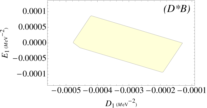
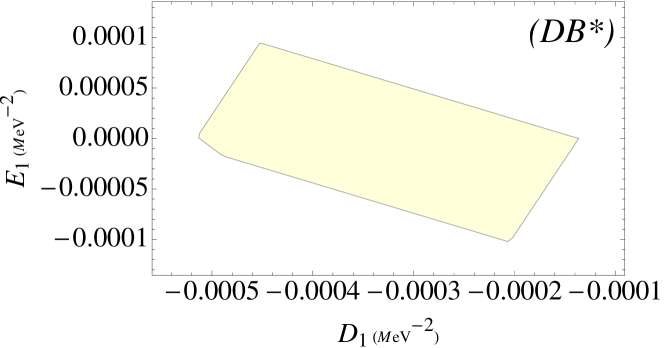
Figure 1: $(D_{1},E_{1})$-parameter space; light shaded areas represent the regions in which the parameters acquire values that allow bound states for the nine states of $SU(3)_{V}$ light-quark flavor basis shown in Eq. (37), with binding energy greater than 0.1 MeV and obeying the condition $a_{S}\gtrsim 3\lambda_{\pi}$. Upper, middle and lower panels represent the $DB({}^{1}S_{0})_{\xi},D^{*}B({}^{3}S_{1})_{\xi}$ and $DB^{*}({}^{3}S_{1})_{\xi}$ systems, respectively ( $\xi=s1,s2,t,d1,d2$ ).

Using this analysis of the $(D_{1},E_{1})$-parameter space, we study the mass, binding energy and scattering length of the $|DB({}^{1}S_{0})\rangle,|D^{*}B({}^{3}S_{1})\rangle$ and $|DB^{*}({}^{3}S_{1})\rangle$ states for different values of the parameters $(D_{1},E_{1})$. These values are chosen in a such way that their magnitudes are smaller, similar or greater than the ones delimited by the intersection region of last panel in Fig. 1:

$(i)$

$D_{1}=-0.000015\;\mathrm{MeV}^{-2},\;E_{1}=-0.00001\;\mathrm{MeV}^{-2}$;

$(ii)$

$D_{1}=-0.00005\;\mathrm{MeV}^{-2},\;E_{1}=-0.00002\;\mathrm{MeV}^{-2}$;

$(iii)$

$D_{1}=-0.0003\;\mathrm{MeV}^{-2},\;E_{1}=-0.00005\;\;\mathrm{MeV}^{-2}$;

$(iv)$

$D_{1}=-0.001\;\mathrm{MeV}^{-2},\;E_{1}=-0.0001\;\mathrm{MeV}^{-2}$.

In general, the choice $(iii)$ works with sufficient magnitudes of $(D_{1},E_{1})$ to be found on the the light shaded area of panels in Fig. 1, while $(i)$ and $(ii)$ [$(iv)$] give magnitudes smaller [greater] than the ones mentioned above and are not inside the mentioned light-shaded region.

The results are shown in Tables LABEL:table2, LABEL:table3 and LABEL:table4 of Appendix A.1. The errors in our predicted quantities are obtained taking into account the violations of heavy quark spin symmetry due to the finite heavy quark mass and the breaking of light flavor symmetry. These effects are the most relevant high-order corrections to the heavy meson contact interactions. For the first of two effects, we expect a relative uncertainty of the order of $\Lambda_{QCD}/m_{Q}$ of the values of $\tilde{V}^{(\alpha)}$ in heavy-quark limit. Taking $\Lambda_{QCD}\sim 200$ MeV and the quark charm mass $m_{c}\sim 1.5$ GeV [15], this estimated error is of 15% in leading order contact interactions. The second deviation, due to $SU(3)$-breaking effects, can be estimated from the ratio of kaon and pion decay constants, $f_{K}/f_{\pi}\sim 1.2$, giving a relative error of 20% in molecules containing strange quarks. Thus, the total error in $\tilde{V}^{(\alpha)}$ is calculated by adding the partial error in quadrature. After that it is possible to estimate the uncertainties in binding energy and in scattering length given by Eqs. (42) and (43), respectively.

In all situations displayed in Tables LABEL:table2, LABEL:table3 and LABEL:table4, the bound states do not seem possible for the choice $(iv)$. On the other hand, we find loosely-bound state solutions for all nine $SU(3)_{V}$ light-quark flavor states ($\xi=s1,s2,t,d1,d2$) in the situation $(iii)$, while in the case of choice (ii) only for the isosinglet $s1$.

Besides, the results suggest that for both spin-0 and spin-1 systems, the $t,d1,d2$ channels present greater binding energies than $s1,s2$ in a specific choice of parameters.

3.2 $D^{*}B^{*}({}^{1}S_{0}),D^{*}B^{*}({}^{3}S_{1})$ and $D^{*}B^{*}({}^{5}S_{2})$ systems

For the $D^{*}B^{*}({}^{1}S_{0}),D^{*}B^{*}({}^{3}S_{1})$ and $D^{*}B^{*}({}^{5}S_{2})$ systems, the parameter space is richer, since the transition amplitudes depend on the constants $C_{1}$ and $C_{2}$, i.e. on $D_{1},E_{1},D_{2}$ and $E_{2}$, according to corresponding channel of effective potential shown in Table 1.

First, we analyze the dependence of bound state solutions with the parameters $(D_{2},E_{2})$. In Figs. 2, 3 and 4 are displayed the $(D_{2},E_{2})$-parameter space for the $D^{*}B^{*}({}^{1}S_{0})_{\xi}$, $D^{*}B^{*}({}^{3}S_{1})_{\xi}$ and $D^{*}B^{*}({}^{5}S_{2})_{\xi}$ systems ($\xi=s1,s2,t,d1,d2$), respectively, taking into account the different choices $(i)-(iv)$ of parameters $(D_{1},E_{1})$ done in previous Section. Light shaded areas represent the regions in which the parameters acquire values that allow bound states for the nine states of $SU(3)_{V}$ light-quark flavor basis shown in Eq. (37), with binding energy greater than 0.1 MeV and obeying the condition $a_{S}\gtrsim 3\lambda_{\pi}$.

These Figures indicate that the change of $(D_{1},E_{1})$ parameters performs a displacement of the light-shaded areas, but without modification of their shapes and surfaces. We remark that in the case of $D^{*}B^{*}({}^{1}S_{0})_{\xi}$, $D^{*}B^{*}({}^{3}S_{1})_{\xi}$ systems, the increasing of magnitude of $(D_{1},E_{1})$ induces a decreasing of values of $(D_{2},E_{2})$ parameters to get bound states. On the other hand, the $D^{*}B^{*}({}^{5}S_{2})_{\xi}$ system presents an inverse behavior: greater values of $(D_{2},E_{2})$ are necessary to yield bound-state solutions as the magnitudes $(D_{1},E_{1})$ grow.

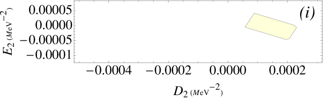
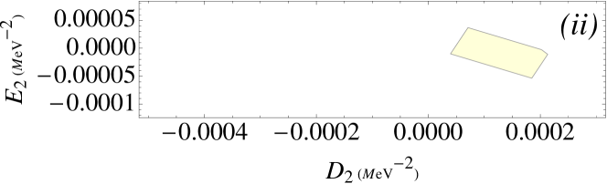
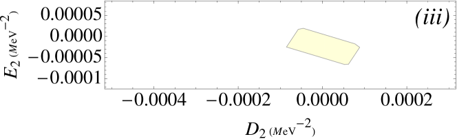
Figure 2: $(D_{2},E_{2})$-parameter space for the $D^{*}B^{*}({}^{1}S_{0})_{\xi}$ system ($\xi=s1,s2,t,d1,d2$). Light shaded areas represent the regions in which the parameters acquire values that allow bound states for the nine states of $SU(3)_{V}$ light-quark flavor basis shown in Eq. (37), with binding energy greater than 0.1 MeV and obeying the condition $a_{S}\gtrsim 3\lambda_{\pi}$. The legends in the panels represent respectively the choices $(i),(ii),(iii)$ and $(iv)$ done in previous Section for the parameters $(D_{1},E_{1})$.

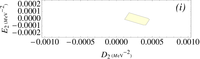
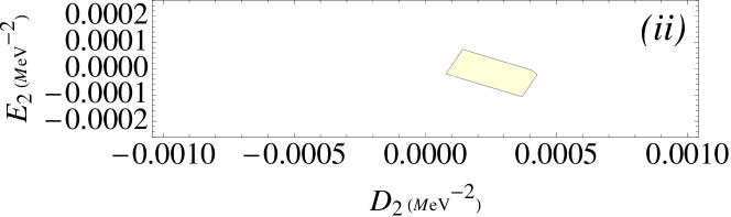
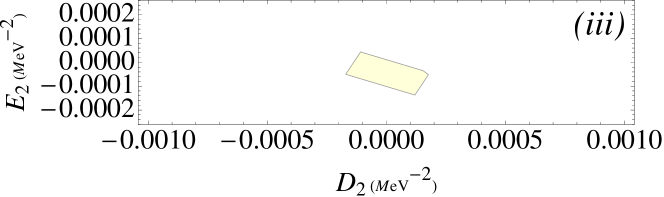
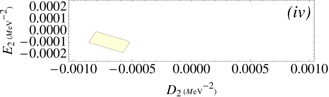
Figure 3: Same as in Fig. 2 for $D^{*}B^{*}({}^{3}S_{1})_{\xi}$ system.

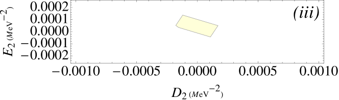
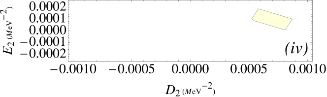
Figure 4: Same as in Fig. 2 for $D^{*}B^{*}({}^{5}S_{2})_{\xi}$ system.

Pursuing our analysis, In Fig. 5 it is shown the $(D_{1},E_{1})$-parameter space for the following values of $(D_{2},E_{2})$:

$(a)$

$D_{2}=0.00001\;\mathrm{MeV}^{-2},\;E_{2}=0.00001\;\mathrm{MeV}^{-2};$

$(b)$

$D_{2}=0.00005\;\mathrm{MeV}^{-2},\;E_{2}=0.000015\;\mathrm{MeV}^{-2};$

$(c)$

$D_{2}=0.00008\;\mathrm{MeV}^{-2},E_{2}=0.00002\;\mathrm{MeV}^{-2}.$

The light shaded areas in Fig. 5 indicate the intersection region in which bound states are obtained for the six studied systems ($DB({}^{1}S_{0})_{\xi}$, $D^{*}B({}^{3}S_{1})_{\xi}$, $DB^{*}({}^{3}S_{1})_{\xi}$, $D^{*}B^{*}({}^{1}S_{0})_{\xi}$, $D^{*}B^{*}({}^{3}S_{1})_{\xi}$ and $D^{*}B^{*}({}^{5}S_{2})_{\xi}$), with binding energy greater than 0.1 MeV and obeying the condition $a_{S}\gtrsim 3\lambda_{\pi}$. The plots suggest that bound-state solutions are inhibited as the magnitude of the constants $(D_{2},E_{2})$ increases.

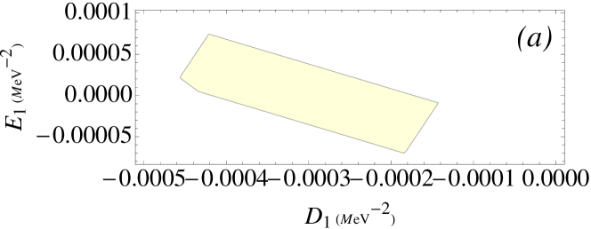
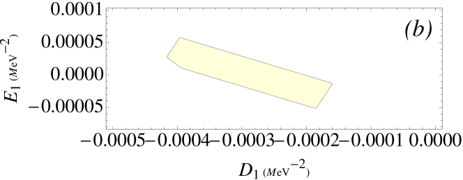
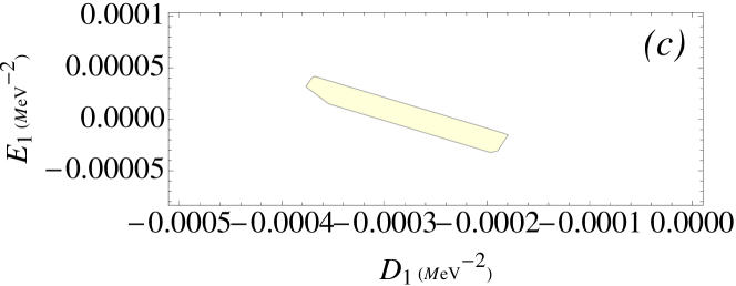
Figure 5: $(D_{1},E_{1})$-parameter space. The light shaded areas indicate the intersection region in which bound states are obtained for the six studied systems ($DB({}^{1}S_{0})_{\xi}$, $D^{*}B({}^{3}S_{1})_{\xi}$, $DB^{*}({}^{3}S_{1})_{\xi}$, $D^{*}B^{*}({}^{1}S_{0})_{\xi}$, $D^{*}B^{*}({}^{3}S_{1})_{\xi}$ and $D^{*}B^{*}({}^{5}S_{2})_{\xi}$), , with binding energy greater than 0.1 MeV and obeying the condition $a_{S}\gtrsim 3\lambda_{\pi}$. $\xi$ represents the nine flavor-state basis shown in Eq. (37). The legends in the panels represent respectively the choices $(a),(b)$ and $(c)$ for the parameters $(D_{2},E_{2})$: $(a)D_{2}=0.00001\;\mathrm{MeV}^{-2},\;E_{2}=0.00001\;\mathrm{MeV}^{-2};$ $(b)D_{2}=0.00005\;\mathrm{MeV}^{-2},\;E_{2}=0.000015\;\mathrm{MeV}^{-2};$ $(c)D_{2}=0.00008\;\mathrm{MeV}^{-2},\;E_{2}=0.00002\;\mathrm{MeV}^{-2}$.

Taking into account the discussion above, we study the mass, binding energy and scattering length of the $D^{*}B^{*}$ systems for $(i)-(iv)$ choices of the parameters $(D_{1},E_{1})$ as in previous section, and at fixed values of $D2=0.00001\mathrm{MeV}^{-2};E2=0.00002\mathrm{MeV}^{-2}$, chosen in order to reproduce the situation of upper-left panel in Fig. 3. The results are shown in Tables LABEL:table5, LABEL:table6 and LABEL:table7 in Appendix A.2. We find loosely-bound state solutions in the following cases:

1. $D^{*}B^{*}({}^{1}S_{0})$: there are loosely bound-state solutions for the $SU(3)_{V}$ light-quark flavor isosinglets $s1$ and $s2$ in the situations $(i)$, $(ii)$ and $(ii)$; for the states $\xi=t,d1,d2$ in the case $(iii)$.

2. $D^{*}B^{*}({}^{3}S_{1})$: there are loosely bound-state solutions for the $SU(3)_{V}$ light-quark flavor isosinglets $s1$ and $s2$ in the situation $(ii)$ and $(iii)$; for the isosinglet $s1$ in the case $(i)$; and for the states $\xi=t,d1,d2$ in the case $(iii)$.

3. $D^{*}B^{*}({}^{5}S_{2})$: bound-state solution exists for all nine $SU(3)$ flavor states ($\xi=s1,s2,t,d1,d2$) only in the situation $(iii)$.

Also, as in the previous Section, the results suggest that for $D^{*}B^{*}({}^{1}S_{0})$ and $D^{*}B^{*}({}^{3}S_{1})$ systems, the $t,d1,d2$ channels present greater binding energies than $s1,s2$ in a specific choice of parameters. In the case of $D^{*}B^{*}({}^{5}S_{2})$, the binding energies are of the same order for a specific set of values of the parameters. Finally, it is important to notice that the number of bound-state solutions shown in Tables LABEL:table5-LABEL:table7 could be lowered for greater values of the parameters $(D_{2},E_{2})$, as indicated in Fig. 5.

3.3 Estimation of Interactions From Experimental Data in Charmonium and Bottomonium Sectors

Although there is no experimental information of exotic states in $B_{c}$ sector, it is also interesting at this point to analyze the parameter space in the light of available experimental data in charmonium and bottomonium sectors. Accordingly, in consonance with Refs. [15, 16] we can use the information available of the $X(3872)$ and $Z_{b}(10610)$ masses as inputs to fix two of the four couplings.

In this sense, we use the analogous approach discussed in previous Sections, by interpreting $X(3872)$ as $S$-wave isoscalar ($J^{PC}=1^{++}$) $D^{0}\bar{D}^{*0}$ molecule (the charged conjugated particles are implicit included) [33]. This channel has the leading-order potential given by $V^{(D^{0}\bar{D}^{*0})}({}^{3}S_{1})=C_{1}+C_{2}$, with $C_{1}=D_{1}+3E_{1},\,C_{2}=D_{2}+3E_{2}$. In the calculations we consider the following central values of $X(3872)$ mass, threshold and binding energy: $M_{X}=3871.69$ MeV [2], $m_{D^{0}}+m_{\bar{D}^{*0}}=3871.8$ MeV [2], and $E_{b}=0.11$ MeV [33], respectively.

Similarly, the $Z_{b}(10610)$ is understood as $S$-wave ($J^{PC}=1^{+-}$) isovector $(B\bar{B}^{*})$ molecule. In this case, the leading-order potential is given by $V^{(B\bar{B}^{*})}({}^{3}S_{1})=C_{1}-C_{2}$, with $C_{1}=D_{1}-E_{1},\,C_{2}=D_{2}-E_{2}$. In alignment with Ref. [16], the binding energy of $Z_{b}(10610)$ is assumed to be $2.0\pm 2.0$ MeV, while its mass and threshold are $M_{Z_{b}}=10602.6\pm 2.0$ MeV and $m_{B}+m_{\bar{B}^{*}}=10604.6$ MeV [2], respectively.

Therefore, using the informations of $X(3872)$ and $Z_{b}(10610)$ in Eqs. (42) and (43), we obtain the following relations

$$D_{1}=-0.00051477+0.5D_{2}-1.5E_{2},$$

$$E_{1}=-0.000422711-0.5D_{2}-0.5E_{2}.$$ (44)

To estimate the two remaining counterterms, we need two more states with different dependence of the couplings with respect to $X(3872)$ and $Z_{b}(10610)$. Following Ref. [15], we consider the $X(3915)$ as a $0^{++}$ isoscalar $(D^{*}\bar{D}^{*})$ molecule, and $Y(4140)$ as a $0^{++}$ $(D_{s}^{*}\bar{D}_{s}^{*})$ molecule, with the leading order potentials given by $V^{(D^{*}\bar{D}^{*})}({}^{1}S_{0})=(D_{1}+3E_{1})-2(D_{2}+3E_{2})$ and $V^{(D_{s}^{*}\bar{D}_{s}^{*})}({}^{1}S_{0})=(D_{1}+E_{1})-2(D_{2}+E_{2})$. The masses and thresholds are $M_{X(3915)}=3917$ MeV, $m_{\bar{D}^{*}}+m_{\bar{D}^{*}}=4017.2$ MeV, $M_{Y(4140)}=4140$ MeV and $m_{\bar{D}^{*}}+m_{\bar{D}^{*}}=4224.6$ MeV. Consequently, the use of these data in Eqs. (42) and (43), in combination with Eq. (44), yields

$$D_{1}=-0.0003973\;\mathrm{MeV}^{-2},\;\;E_{1}=0.00027\;\mathrm{MeV}^{-2},\;$$

$$D_{2}=-0.00017037\;\mathrm{MeV}^{-2},\;E_{2}=-0.0001351\;\mathrm{MeV}^{-2}.$$ (45)

Hence, with this specific renormalization scheme we can estimate the quantities of the $D^{(*)}B^{(*)}$ states. The results are displayed in Appendix A.3. We remark that in this situation we have computed the total error by adding the partial errors (due to violations of heavy-quark spin and light flavor symmetries and in $Z_{b}(10610)$ binding energy) in quadratures. We see in general a pattern of loosely bound states from these outcomes.

It is worth remarking that the choice of $X(3915)$ and $Y(4140)$ have some troubles, as greater binding energies and experimental status, as observed in Ref. [15]. In this sense, the predictions generated from this choice will remain matter of debate. In addition, we stress that the renormalization procedure should be performed in each sector, and that there is not yet experimental evidence of hadronic molecules with both open charm and open bottom to have more solid predictions.

4 Discussion and Concluding Remarks

In summary, we have investigated the interaction between charmed and bottomed mesons using Heavy-Meson Effective Theory. In this scenario we have discussed the formation deuteron-like molecules with both open charm and bottom. We have explored the regions in parameter space of the coupling constants in which the formation of bound $D^{(*)}B^{(*)}$-states are allowed. Estimations of their masses, binding energies and scattering lengths have been performed as functions of interaction strength in a specific renormalization scheme. We have worked here in a specific renormalization scheme, in which the relation between the bare coupling constants is conserved after renormalization. This approach has allowed to relate the results for different sectors, taking into account the fact that there is not yet experimental evidence of hadronic molecules with both open charm and open bottom.

The analysis of bound-state solutions of $D^{(*)}B^{(*)}$ has been restricted to the region of relevance of contact-range interaction, in which the pion-exchange contribution is not relevant. In this sense, we have studied bound states which obey the condition $a_{S}\gtrsim 3\lambda_{\pi}$.

The study is simpler and more direct for $DB({}^{1}S_{0}),D^{*}B({}^{3}S_{1})$ and $DB^{*}({}^{3}S_{1})$ systems, since they depend on two of the four coupling constants in Effective Lagrangian. In this context, the analysis of the parameter space has indicated a region in which the relevant parameters acquire values that allow loosely bound states for some of the nine $SU(3)_{V}$ light-quark flavor states (two isosinglets, one triplet and two doublets). The results suggested that for both spin-0 and spin-1 systems, the $t,d1,d2$ channels present greater binding energies than $s1,s2$ in a specific choice of parameters.

For the $D^{*}B^{*}({}^{1}S_{0}),D^{*}B^{*}({}^{3}S_{1})$ and $D^{*}B^{*}({}^{5}S_{2})$ systems, the parameter configuration space is richer, since the transition amplitudes depend on the four coupling constants. This study has suggested, as in the above mentioned situation, that the existence of loosely bound states for the $SU(3)_{V}$ light-quark flavor states strongly depends on the magnitude of the parameters. In the case of $D^{*}B^{*}({}^{1}S_{0})_{\xi}$, $D^{*}B^{*}({}^{3}S_{1})_{\xi}$ systems, for a specific choice of renormalization scheme the increasing of magnitude of $(D_{1},E_{1})$ induces a decreasing of values of $(D_{2},E_{2})$ parameters in order to get bound states; while with $D^{*}B^{*}({}^{5}S_{2})_{\xi}$ system this dependence is inverse: greater values of $(D_{2},E_{2})$ are necessary to yield bound-state solutions.

In addition, the $D^{(*)}B^{(*)}$ states have also analyzed with a specific renormalization scheme, in which the couplings have been fixed by considering the location of $X(3872)$, $Z_{b}(10610)$, $X(3915)$ and $Y(4140)$ states, interpreted here as heavy-meson molecules. The results obtained with this specific choice reveal in general a pattern of loosely bound states.

We notice that some results reported above can be compared with other ones available in literature. For example, the state $|D^{*}B^{*}({}^{5}S_{2})_{s1}\rangle$ with the parameters assuming values between the choices $(ii)$ and $(iii)$ displayed in table LABEL:table7 has its mass in the range of the outcome obtained in Ref. [16]. In addition, the mass yielded for the state $|D^{*}B^{*}({}^{3}S_{1})_{t}\rangle$ in the case $(iii)$ of Table LABEL:table6, is in the range of the equivalent state discussed in Ref. [16]. If we compare with the specific renormalization scheme shown in Eq. (45), fixed to location of observed exotic states in charmonium and bottomonium sectors, we see that our findings in Table LABEL:table8 for the $|D^{*}B^{*}({}^{3}S_{1})_{t}\rangle$ state are in the range of the results in Ref. [16], but in the case of $|D^{*}B^{*}({}^{5}S_{2})_{s1}\rangle$ our estimation yields a very loosely bound state.

Furthermore, bound-state solutions pointed out in Ref. [23] can be discussed in some sense under our point of view, with the parameters in the range of the choices $(i)$ and $(ii)$ of Tables LABEL:table2-LABEL:table7. Notice, however, that Ref. [23] has considered mixing S-D mixing effect, and we must be careful in this comparison.

Further work is needed to improve these results, in order to perform more precise comparison with other phenomenological models, and to contribute to the experimental search of $D^{(*)}B^{(*)}$ molecular states. It is possible, for example, to study the decays of these predicted molecular states into $B_{c}$ mesons and light mesons, as suggested in Ref. [23]. Another improvement is the inclusion of the pion-exchange potential, in order to extend the range of applicability of this approach.

ACKNOWLEDGMENTS

We thank CAPES and CNPq (Brazilian Agencies) for financial support.

Appendix A Appendix

A.1 Quantities for the $DB({}^{1}S_{0})_{\xi},D^{*}B({}^{3}S_{1})_{\xi}$ and $DB^{*}({}^{3}S_{1})_{\xi}$ systems for different values of $(D_{1},E_{1})$

Table 2: Relevant quantities for the $DB({}^{1}S_{0})_{\xi}$ system ($\xi=s1,s2,t,d1,d2$ represent the nine flavor states shown in Eq. (37)). $M_{Th}$, $M$, B.E., and $a_{s}$ mean threshold, mass, binding energy and scattering length of the respective state. The parameters $(D_{1},E_{1})$ are chosen in the four situations: $(i)D_{1}=-0.000015\;\mathrm{MeV}^{-2},\;E_{1}=-0.00001\;\mathrm{MeV}^{-2};(ii)D_{1}=-0.00005\;\mathrm{MeV}^{-2},\;E_{1}=-0.00002\;\mathrm{MeV}^{-2};(iii)D_{1}=-0.0003\;\mathrm{MeV}^{-2},E_{1}=-0.00005\;\mathrm{MeV}^{-2};(iv)D_{1}=-0.001\;\mathrm{MeV}^{-2},\;E_{1}=-0.0001\;\mathrm{MeV}^{-2}.$ Bold columns indicate states with binding energy greater than 0.1 MeV and obeying the condition $a_{S}\gtrsim 3\lambda_{\pi}$.

$\xi$	$M_{Th}$ (MeV)	$(D_{1},E_{1})$	$M$ (MeV)	B.E. (MeV)	$a_{s}$ (fm)
$s1$	7146.6	(i)	7133.7 $\pm$ 3.9	12.9 $\pm$3.9	1.1 $\pm$ 0.2
		(ii)	7144.4 $\pm$ 0.7	2.2 $\pm$ 0.7	2.6 $\pm$ 0.4
		(iii)	7146.5 $\pm$ 0.1	0.1 $\pm$0.1	10.3 $\pm$ 1.5
		(iv)	7146.58 $\pm$ 0.01	0.02 $\pm$ 0.01	29.3 $\pm$ 4.4
${s2}$	7335.3	(i)	7302.4 $\pm$ 16.5	32.9$\pm$ 16.5	0.7$\pm$ 0.2
		(ii)	7330.8 $\pm$ 2.3	4.5 $\pm$ 2.3	1.8 $\pm$ 0.4
		(iii)	7335.1$\pm$ 0.1	0.2 $\pm$ 0.1	8.4 $\pm$ 2.1
		(iv)	7335.28 $\pm$ 0.01	0.02 $\pm$ 0.01	26 $\pm$ 6.5
${t}$	7146.6	(i)	6713.4 $\pm$ 130	433.2 $\pm$ 130	0.2$\pm$ 0.02
		(ii)	7124.2 $\pm$ 6.7	22.4 $\pm$ 6.7	0.8$\pm$ 0.1
		(iii)	7146.2 $\pm$ 0.2	0.4 $\pm$ 0.2	5.9 $\pm$ 0.8
		(iv)	7146.57 $\pm$ 0.01	0.03 $\pm$ 0.01	20.5 $\pm$ 3
${d1}$	7247.9	(i)	6862.2 $\pm$ 192	385.7 $\pm$ 192	0.2 $\pm$ 0.1
		(ii)	7223 $\pm$ 10	19.9 $\pm$ 10	0.8 $\pm$ 0.2
		(iii)	7247.5 $\pm$ 0.2	0.4 $\pm$ 0.2	6.1 $\pm$ 1.5
		(iv)	7247.87 $\pm$ 0.01	0.03 $\pm$ 0.01	21.3 $\pm$ 5.3
${d2}$	7234	(i)	6806.3 $\pm$ 213	427.7 $\pm$ 213	0.2 $\pm$ 0.1
		(ii)	7211.9 $\pm$ 11	22.1 $\pm$ 11	0.8 $\pm$ 0.2
		(iii)	7233.6 $\pm$ 0.2	0.4 $\pm$ 0.2	5.9 $\pm$ 1.5
		(iv)	7233.97 $\pm$ 0.02	0.03 $\pm$ 0.2	20.6 $\pm$ 5.1

Table 3: Same as in table LABEL:table2 for $D^{*}B({}^{3}S_{1})_{\xi}$ system.

$\xi$	$M_{Th}$ (MeV)	$(D_{1},E_{1})$	$M$(MeV)	B.E. (MeV)	$a_{s}$ (fm)
${s1}$	7288.	(i)	7277 $\pm$ 3.3	10.972 $\pm$ 11	1.1 $\pm$ 0.2
		(ii)	7286.1 $\pm$ 0.6	1.9 $\pm$ 0.6	2.7 $\pm$ 0.4
		(iii)	7287.9 $\pm$ 0.04	0.1 $\pm$ 0.04	10.8 $\pm$ 1.6
		(iv)	7287.99 $\pm$ 0.01	0.01 $\pm$ 0.01	30.9 $\pm$ 4.6
${s2}$	7479.1	(i)	7450.8 $\pm$ 14.1	28.2$\pm$ 14.1	0.7 $\pm$ 0.2
		(ii)	7475.2 $\pm$ 1.9	3.9 $\pm$ 1.9	1.5 $\pm$ 0.5
		(iii)	7478.9 $\pm$ 0.1	0.2 $\pm$ 0.1	8.8 $\pm$ 2.2
		(iv)	7479.09 $\pm$ 0.01	0.01 $\pm$ 0.01	27.3 $\pm$ 6.8
${t}$	7288	(i)	6918.9 $\pm$ 110.7	369.1 $\pm$ 110.7	0.2 $\pm$ 0.1
		(ii)	7268.9 $\pm$ 5.7	19.1 $\pm$ 5.7	0.9 $\pm$ 0.1
		(iii)	7287.6 $\pm$ 0.1	0.4 $\pm$ 0.1	6.2 $\pm$ 0.9
		(iv)	7287.97 $\pm$ 0.01	0.03 $\pm$ 0.01	21.6 $\pm$ 3.2
${d1}$	7391.7	(i)	7060.6 $\pm$ 165.6	331.1 $\pm$ 165.6	0.2 $\pm$ 0.1
		(ii)	7374.6 $\pm$ 8.6	17.1 $\pm$ 8.6	0.9 $\pm$ 0.2
		(iii)	7391.4 $\pm$ 0.2	0.3 $\pm$ 0.2	6.4 $\pm$ 1.6
		(iv)	7391.67 $\pm$ 0.01	0.03 $\pm$ 0.01	22.4 $\pm$ 5.6
${d2}$	7375.4	(i)	7011.3 $\pm$ 182.1	364.1 $\pm$ 182.1	0.2 $\pm$ 0.5
		(ii)	7356.6 $\pm$ 9.4	18.8 $\pm$ 9.4	0.9 $\pm$ 0.2
		(iii)	7375 $\pm$ 0.2	0.4 $\pm$ 0.2	6.2 $\pm$ 2.6
		(iv)	7375.37 $\pm$ 0.01	0.03 $\pm$ 0.1	21.7 $\pm$ 5.4

Table 4: Same as in table LABEL:table2 for $DB^{*}({}^{3}S_{1})_{\xi}$ system.

$\xi$	$M_{Th}$ (MeV)	$(D_{1},E_{1})$	$M$ (MeV)	B.E. (MeV)	$a_{s}$ (fm)
${s1}$	7192.4	(i)	7179.6 $\pm$ 3.8	12.8 $\pm$ 3.8	1.1 $\pm$ 0.2
		(ii)	7190.2 $\pm$ 0.7	2.2 $\pm$ 0.7	2.6 $\pm$ 0.4
		(iii)	7192.3 $\pm$ 0.4	0.1 $\pm$ 0.4	10.3 $\pm$ 1.5
		(iv)	7192.38 $\pm$ 0.01	0.02 $\pm$ 0.1	29.3 $\pm$ 4.4
${s2}$	7383.9	(i)	7351.2 $\pm$ 16.3	32.7 $\pm$ 16.3	0.7 $\pm$ 0.2
		(ii)	7379.4 $\pm$ 2.2	4.5 $\pm$ 2.2	1.8 $\pm$ 0.4
		(iii)	7383.7 $\pm$ 0.1	0.2 $\pm$ 0.1	8.4 $\pm$ 2.1
		(iv)	7383.88 $\pm$ 0.01	0.02 $\pm$ 0.01	26 $\pm$ 6.5
${t}$	7192.4	(i)	6762.1 $\pm$ 129.1	430.3 $\pm$ 129.1	0.2 $\pm$ 0.03
		(ii)	7170.2 $\pm$ 6.7	22.2 $\pm$ 6.7	0.8 $\pm$ 0.1
		(iii)	7192 $\pm$ 0.1	0.4 $\pm$ 0.1	5.9 $\pm$ 0.9
		(iv)	7192.37 $\pm$ 0.01	0.03 $\pm$ 0.01	20.5 $\pm$ 3.1
${d1}$	7293.7	(i)	6910.7 $\pm$ 191.5	383 $\pm$ 191.5	0.2 $\pm$ 0.1
		(ii)	7273.9 $\pm$ 9.9	19.8 $\pm$ 9.9	0.8 $\pm$ 0.2
		(iii)	7293.3 $\pm$ 0.2	0.4 $\pm$ 0.2	6.1 $\pm$ 1.5
		(iv)	7293.67 $\pm$ 0.2	0.03 $\pm$ 0.2	21.3 $\pm$ 5.3
${d2}$	7282.6	(i)	6857.8 $\pm$ 212.4	424.8 $\pm$ 212.4	0.2 $\pm$ 0.1
		(ii)	7260.7 $\pm$ 11	21.9 $\pm$ 11	0.8 $\pm$ 0.2
		(iii)	7282.2 $\pm$ 0.2	0.4 $\pm$ 0.2	5.9 $\pm$ 1.5
		(iv)	7282.57 $\pm$ 0.2	0.03 $\pm$ 0.2	20.6 $\pm$ 5.2

A.2 Quantities for the $D^{*}B^{*}({}^{1}S_{0})_{\xi},D^{*}B^{*}({}^{3}S_{1})_{\xi}$ and $D^{*}B^{*}({}^{5}S_{2})_{\xi}$ systems for different values of $(D_{1},E_{1})$

Table 5: Same as in table LABEL:table2 for $D^{*}B^{*}({}^{1}S_{0})_{\xi}$ system, with ($D2=0.00001\;\mathrm{MeV}^{-2};\;E2=0.00002\;\mathrm{MeV}^{-2}$).

$\xi$	$M_{Th}$ (MeV)	$(D_{1},E_{1})$	$M$ (MeV)	B.E. (MeV)	$a_{s}$ (fm)
${s1}$	7333.8	(i)	7333.2 $\pm$ 0.2	0.6 $\pm$ 0.2	4.7 $\pm$ 0.7
		(ii)	7333.5 $\pm$ 0.1	0.3 $\pm$ 0.1	6.3 $\pm$ 0.9
		(iii)	7333.7 $\pm$ 0.2	0.1 $\pm$ 0.2	14.4 $\pm$ 2.2
		(iv)	7333.79 $\pm$ 0.01	0.01 $\pm$ 0.01	34.5 $\pm$ 5.2
${s2}$	7527.7	(i)	7525.5 $\pm$ 1.1	2.2 $\pm$ 1.1	2.5 $\pm$ 0.6
		(ii)	7526.7 $\pm$ 0.5	1 $\pm$ 0.5	3.6 $\pm$ 0.9
		(iii)	7527.6 $\pm$ 0.1	0.1 $\pm$ 0.1	10.6 $\pm$ 2.7
		(iv)	7527.68 $\pm$ 0.01	0.02 $\pm$ 0.01	29.2 $\pm$ 7.3
${t}$	7333.8	(i)	-	-	-
		(ii)	7305.5 $\pm$ 8.5	28.3 $\pm$ 8.5	0.7 $\pm$ 0.1
		(iii)	7333.4 $\pm$ 0.1	0.4 $\pm$ 0.1	6 $\pm$ 0.9
		(iv)	7333.77 $\pm$ 0.01	0.03 $\pm$ 0.01	21.5 $\pm$ 3.2
${d1}$	7437.5	(i)	-	-	-
		(ii)	7412.1 $\pm$ 12.7	25.4 $\pm$ 12.7	0.7 $\pm$ 0.2
		(iii)	7437.2 $\pm$ 0.2	0.3 $\pm$ 0.2	6.3 $\pm$ 1.6
		(iv)	7437.47 $\pm$ 0.01	0.03 $\pm$ 0.01	22.3 $\pm$ 5.6
${d2}$	7424	(i)	-	-	-
		(ii)	7396.1 $\pm$ 13.9	27.9 $\pm$ 13.9	0.7 $\pm$ 0.2
		(iii)	7423.6 $\pm$ 0.2	0.4 $\pm$ 0.2	6.1 $\pm$ 1.5
		(iv)	7423.97 $\pm$ 0.01	0.03 $\pm$ 0.01	21.6 $\pm$ 5.4

Table 6: Same as in table LABEL:table2 for $D^{*}B^{*}({}^{3}S_{1})_{\xi}$ system, with ($D2=0.00001\;\mathrm{MeV}^{-2};\;E2=0.00002\;\mathrm{MeV}^{-2}$).

$\xi$	$M_{Th}$ (MeV)	$(D_{1},E_{1})$	$M$ (MeV)	B.E. (MeV)	$a_{s}$ (fm)
${s1}$	7333.8	(i)	7332.2 $\pm$ 0.5	1.6 $\pm$ 0.5	2.9 $\pm$ 0.4
		(ii)	7333.1 $\pm$ 0.2	0.7 $\pm$ 0.2	4.5 $\pm$ 0.6
		(iii)	7333.7 $\pm$ 0.03	0.1 $\pm$ 0.03	12.6 $\pm$ 1.9
		(iv)	7333.79 $\pm$ 0.01	0.01 $\pm$ 0.01	32.7 $\pm$ 4.9
${s2}$	7527.7	(i)	7522.4 $\pm$ 2.7	5.3 $\pm$ 2.7	1.6 $\pm$ 0.4
		(ii)	7525.9 $\pm$ 0.9	1.8 $\pm$ 0.9	2.7 $\pm$ 0.7
		(iii)	7527.5 $\pm$ 0.1	0.2 $\pm$ 0.1	9.8 $\pm$ 2.4
		(iv)	7527.68 $\pm$ 0.01	0.02 $\pm$ 0.01	28.3 $\pm$ 7.1
${t}$	7333.8	(i)	6315.8 $\pm$ 305.4	1018 $\pm$ 305.4	0.1 $\pm$ 0.02
		(ii)	7310.9 $\pm$ 6.9	22.9 $\pm$ 6.9	0.8 $\pm$ 0.2
		(iii)	7333.4 $\pm$ 0.1	0.4 $\pm$ 0.1	6.1 $\pm$ 0.9
		(iv)	7333.77 $\pm$ 0.1	0.03 $\pm$ 0.01	21.6 $\pm$ 3.2
${d1}$	7437.5	(i)	6524.5 $\pm$ 456.5	913 $\pm$ 456.5	0.1 $\pm$ 0.03
		(ii)	7417 $\pm$ 10.3	20.5 $\pm$ 10.3	0.8 $\pm$ 0.2
		(iii)	7437.2 $\pm$ 0.2	0.3 $\pm$ 0.2	6.3 $\pm$ 1.6
		(iv)	7437.47 $\pm$ 0.1	0.03 $\pm$ 0.1	22.4 $\pm$ 5.6
${d2}$	7424	(i)	6419.9 $\pm$ 502.1	1004.1 $\pm$ 502.1	0.1 $\pm$ 0.03
		(ii)	7401.4 $\pm$ 11.3	22.6 $\pm$ 11.3	0.8 $\pm$ 0.2
		(iii)	7423.6 $\pm$ 0.2	0.4 $\pm$ 0.2	6.1 $\pm$ 1.5
		(iv)	7423.7 $\pm$ 0.1	0.03 $\pm$ 0.1	21.7 $\pm$ 5.4

Table 7: Same as in table LABEL:table2 for $D^{*}B^{*}({}^{5}S_{2})_{\xi}$ system, with ($D2=0.00001\;\mathrm{MeV}^{-2};E2=0.00002\;\mathrm{MeV}^{-2}$).

$\xi$	$M_{Th}$ (MeV)	$(D_{1},E_{1})$	$M$ (MeV)	B.E. (MeV)	$a_{s}$ (fm)
${s1}$	7333.8	(i)	-	-	-
		(ii)	7317.9 $\pm$ 4.8	15.9 $\pm$ 4.8	0.9 $\pm$ 0.1
		(iii)	7333.6 $\pm$ 0.1	0.2 $\pm$ 0.1	9.1 $\pm$ 1.4
		(iv)	7333.78 $\pm$ 0.01	0.02 $\pm$ 0.01	29.2 $\pm$ 4.3
${s2}$	7527.7	(i)	-	-	-
		(ii)	7513.6 $\pm$ 7	14.1 $\pm$ 7	1 $\pm$ 0.2
		(iii)	7527.5 $\pm$ 0.1	0.2 $\pm$ 0.1	8 $\pm$ 2
		(iv)	7527.68 $\pm$ 0.01	0.02 $\pm$ 0.01	26.5 $\pm$ 6.6
${t}$	7333.8	(i)	7146.8 $\pm$ 56	187 $\pm$ 56	0.3 $\pm$ 0.1
		(ii)	7317.9 $\pm$ 4.8	15.9 $\pm$ 4.8	0.9 $\pm$ 0.1
		(iii)	7333.4 $\pm$ 0.1	0.5 $\pm$ 0.1	6.3 $\pm$ 0.9
		(iv)	7333.77 $\pm$ 0.01	0.03 $\pm$ 0.01	21.7 $\pm$ 3.3
${d1}$	7437.5	(i)	7269.8 $\pm$ 83.8	167.7 $\pm$ 83.8	0.3 $\pm$ 0.1
		(ii)	7423.2 $\pm$ 7.1	14.3 $\pm$ 7.1	1 $\pm$ 0.2
		(iii)	7437.2 $\pm$ 0.2	0.3 $\pm$ 0.2	6.5 $\pm$ 1.6
		(iv)	7437.47 $\pm$ 0.01	0.03 $\pm$ 0.01	22.5 $\pm$ 5.6
${d2}$	7424	(i)	7239.6 $\pm$ 92.2	184.4 $\pm$ 92.2	0.3 $\pm$ 0.1
		(ii)	7408.3 $\pm$ 7.8	15.7 $\pm$ 7.8	0.9 $\pm$ 0.2
		(iii)	7423.7 $\pm$ 0.2	0.3 $\pm$ 0.2	6.3 $\pm$ 1.6
		(iv)	7423.97 $\pm$ 0.01	0.03 $\pm$ 0.01	21.8 $\pm$ 5.5

A.3 Quantities for the $D^{(*)}B^{(*)}$ systems for fixed values of $(D_{1},E_{1},D_{2},E_{2})$ obtained from inputs

Table 8: Relevant quantities for the $D^{(*)}B^{(*)}$ systems. The parameters $(D_{1},E_{1},D_{2},E_{2})$ are chosen in the situation: $D_{1}=-0.0003973\;\mathrm{MeV}^{-2},\;D_{2}=0.00027\;\mathrm{MeV}^{-2},\;D_{2}=-0.00017037\;\mathrm{MeV}^{-2},\;E_{2}=-0.0001351\;\mathrm{MeV}^{-2}$. $M_{Th}$, $M$, B.E., and $a_{s}$ mean threshold, mass, binding energy and scattering length of the respective state.

State	$\xi$	$M_{Th}$ (MeV)	$M$ (MeV)	B. E. (MeV)	$a_{s}$ (fm)
$DB({}^{1}S_{0})$	$s1$	7146.6	7146.58 $\pm$ 0.01	0.02 $\pm$ 0.01	28.5 $\pm$ 6.9
	$s2$	7335.3	7335.3	-	-
	$t$	7146.6	7146 $\pm$ 0.3	0.6 $\pm$ 0.3	4.8 $\pm$ 0.9
	$d1$	7247.9	7247.3 $\pm$ 0.3	0.6 $\pm$ 0.3	5 $\pm$ 1.4
	$d2$	7234	7233.4 $\pm$ 0.4	0.6 $\pm$ 0.4	4.8 $\pm$ 1.3
$D^{*}B({}^{3}S_{1})$	$s1$	7288	7287.98 $\pm$ 0.01	0.02 $\pm$ 0.01	30 $\pm$ 4.9
	$s2$	7479.1	7479.06 $\pm$ 0.02	0.04 $\pm$ 0.02	18.3 $\pm$ 4.7
	$t$	7288	7287.5 $\pm$ 0.2	0.5 $\pm$ 0.2	5 $\pm$ 1
	$d1$	7391.7	7391.2 $\pm$ 0.3	0.5 $\pm$ 0.3	5.2 $\pm$ 1.5
	$d2$	7375.4	7374.9 $\pm$ 0.3	0.5 $\pm$ 0.3	5.1 $\pm$ 1.4
$DB^{*}({}^{3}S_{1})$	$s1$	7192.4	7192.38 $\pm$ 0.01	0.02 $\pm$ 0.01	28.5 $\pm$ 4.6
	$s2$	7383.9	7383.8 $\pm$ 0.02	0.02 $\pm$ 0.02	17.4 $\pm$ 4.4
	$t$	7192.4	7191.8 $\pm$ 0.3	0.6 $\pm$ 0.3	4.8 $\pm$ 0.9
	$d1$	7293.7	7293.1 $\pm$ 0.3	0.6 $\pm$ 0.3	5 $\pm$ 1.4
	$d2$	7282.6	7282 $\pm$ 0.3	0.6 $\pm$ 0.3	4.8 $\pm$ 1.4
$D^{*}B^{*}({}^{1}S_{0})$	$s1$	7333.8	7325.6 $\pm$ 33.5	8.2 $\pm$ 33.5	1.3 $\pm$ 2.6
	$s2$	7527.7	7520.6 $\pm$ 14.2	7.1 $\pm$ 14.2	1.4 $\pm$ 1.4
	$t$	7333.8	7325.9 $\pm$ 11.2	7.9 $\pm$ 11.2	1.3 $\pm$ 0.9
	$d1$	7437.5	7430.4 $\pm$ 10.4	7.1 $\pm$ 10.4	1.4 $\pm$ 1
	$d2$	7424	7416.2 $\pm$ 11.4	7.8 $\pm$ 11.4	1.3 $\pm$ 1
$D^{*}B^{*}({}^{3}S_{1})$	$s1$	7333.8	7333.7 $\pm$ 0.03	0.1 $\pm$ 0.02	15.7 $\pm$ 3.5
	$s2$	7527.7	7527.6 $\pm$ 0.1	0.1 $\pm$ 0.1	9.8 $\pm$ 2.8
	$t$	7333.8	7332.4 $\pm$ 0.9	1.4 $\pm$ 0.9	3.1 $\pm$ 1
	$d1$	7437.5	7436.3 $\pm$ 0.9	1.2 $\pm$ 0.9	3.3 $\pm$ 1.3
	$d2$	7424	7422.7 $\pm$ 0.8	1.3 $\pm$ 0.8	3.2 $\pm$ 0.9
$D^{*}B^{*}({}^{5}S_{2})$	$s1$	7333.8	7333.79 $\pm$ 0.01	0.01 $\pm$ 0.01	44.5 $\pm$ 7.2
	$s2$	7527.7	7527.68 $\pm$ 0.01	0.2 $\pm$ 0.01	26.8 $\pm$ 6.8
	$t$	7333.8	7333.5 $\pm$ 0.1	0.3 $\pm$ 0.1	6.9 $\pm$ 1.4
	$d1$	7437.5	7437.2 $\pm$ 0.1	0.3 $\pm$ 0.1	7.2 $\pm$ 2
	$d2$	7424	7423.7 $\pm$ 0.2	0.3 $\pm$ 0.2	6.9 $\pm$ 2

References

- [1] N. Brambilla et al., Eur. Phys. J. C 71 (2011) 1534, arXiv:1010.5827 [hep-ph].
- [2] K.A. Olive et al. (Particle Data Group), Chin. Phys. C 38 (2014) 090001.
- [3] For a summary of proposed models and interpretations, see Table 20 from Ref. [1].
- [4] M.B. Voloshin and L. B. Okun, JETP Lett. 23 (1976) 333.
- [5] N.A. Tornqvist, Nuovo Cim. A 107 (1994) 2471, arXiv:hep-ph /9310225 [hep-ph].
- [6] N.A. Tornqvist, Z. Phys. C 61 (1994) 525, arXiv:hep-ph /9310247.
- [7] N. A. Tornqvist, Phys. Lett. B 590 (2004) 209, arXiv:hep-ph/0402237.
- [8] M.T. Alfiky, F. Gabbiani and A. A. Petrov, Phys. Lett. B 640 (2006) 238, arXiv:hep-ph/0506141.
- [9] E. Braaten and M. Lu, Phys. Rev. D 76 (2007) 094028, arXiv:0709.2697 [hep-ph].
- [10] Y. b. Dong, A. Faessler, T. Gutsche, and V. E. Lyubovitskij, Phys. Rev. D 77 (2008) 094013, arXiv:0802.3610 [hep-ph].
- [11] Y. Dong, A. Faessler, T. Gutsche, S. Kovalenko, and V. E. Lyubovitskij, Phys. Rev. D 79 (2009) 094013, arXiv:0903.5416 [hep-ph].
- [12] I. W. Lee, A. Faessler, T. Gutsche, and V. E. Lyubovitskij, Phys. Rev. D 80 (2009) 094005, arXiv:0910.1009 [hep-ph].
- [13] E. Braaten and J. Stapleton, Phys. Rev. D 81 (2010) 014019, arXiv:0907.3167 [hep-ph].
- [14] J. Nieves and M.P. Valderrama, Phys. Rev. D 86 (2012) 056004, arXiv:1204.2790.
- [15] C. Hidalgo-Duque, J. Nieves, M. Pavon Valderrama, Phys. Rev. D 87 (2013) 076006, arXiv:1210.5431 [hep-ph].
- [16] F.-K Guo, C. Hidalgo-Duque, J. Nieves, M. P. Valderrama, Phys. Rev. D 88 (2013) 054007, arXiv:1303.6608 [hep-ph].
- [17] A. Martinez Torres, K. P. Khemchandani, F. S. Navarra, M. Nielsen, L. M. Abreu, Phys. Rev. D 90 (2014) 114023, arXiv:1405.7583 [hep-ph].
- [18] A. Bondar, A. Garmash, A. Milstein, R. Mizuk, and M. Voloshin, Phys.Rev. D 84 (2011) 054010, arXiv:1105.4473 [hep-ph].
- [19] M. Cleven, Q. Wang, F.-K. Guo, C. Hanhart, U.-G. Meissner, and Q. Zhao, Phys.Rev. D 87 (2013) 074006, arXiv:1301.6461 [hep-ph].
- [20] R. M. Albuquerque and M. Nielsen, Nucl. Phys. A 815 (2009) 53, arXiv:0804.4817 [hep-ph].
- [21] G.-J. Ding, Phys.Rev. D 79 (2009) 014001, arXiv:0809.4818 [hep-ph].
- [22] Q. Wang, C. Hanhart, and Q. Zhao, (2013), Phys. Rev. Lett. 111 (2013) 132003, arXiv:1303.6355 [hep-ph].
- [23] Z.-F. Sun, X. Liu, M. Nielsen, S.-L. Zhu, Phys. Rev. D 85 (2012) 094008, arXiv:1203.1090 [hep-ph].
- [24] J.-R. Zhang, M.-Q. Huang, Phys. Rev. D 80 (2009) 056004, arXiv:0906.0090 [hep-ph].
- [25] R.M. Albuquerque, X. Liu, M. Nielsen, Phys. Lett. B 718 (2012) 492, arXiv:1203.6569 [hep-ph].
- [26] N. Li, Z.-F. Sun, X. Liu, S.-L. Zhu, Phys. Rev. D 88 (2013) 114008, arXiv:1211.5007 [hep-ph].
- [27] A.V. Manohar, M.B. Wise, Heavy quark physics , Cambridge Monographs on Particle Physics, Nuclear Physics, and Cosmology (Cambridge University Press, Cambridge, 2000).
- [28] M.P. Valderrama, Phys.Rev. D 85 (2012) 114037, arXiv:1204.2400.
- [29] Z.-W. Liu, N. Li, S.-L. Zhu, Phys. Rev. D 89 (2014) 074015.
- [30] R. Casalbuoni, A. Deandrea, N. Di Bartolomeo, R. Gatto, F. Feruglio, G. Nardulli, Phys. Rept. 281 (1997) 145.
- [31] M.C. Birse, Phys. Rev. C 74 (2006) 014003, arXiv:nucl-th/0507077.
- [32] E. Epelbaum, H.-W. Hammer, U.-G. Meissner, Rev. Mod. Phys. 81 (2009) 1773, arXiv:0811.1338 [nucl-th].
- [33] A. Esposito, A. L. Guerrieri, F. Piccinini, A. Pilloni and A. P. Polosa, Int. J. Mod. Phys. A 30 (2015) 1530002, arXiv:1411.5997 [hep-ph].