Proximal Operators for Multi-Agent Path Planning

Abstract

We address the problem of planning collision-free paths for multiple agents using optimization methods known as proximal algorithms. Recently this approach was explored in ? (?), which demonstrated its ease of parallelization and decentralization, the speed with which the algorithms generate good quality solutions, and its ability to incorporate different proximal operators, each ensuring that paths satisfy a desired property. Unfortunately, the operators derived only apply to paths in 2D and require that any intermediate waypoints we might want agents to follow be preassigned to specific agents, limiting their range of applicability. In this paper we resolve these limitations. We introduce new operators to deal with agents moving in arbitrary dimensions that are faster to compute than their 2D predecessors and we introduce landmarks, space-time positions that are automatically assigned to the set of agents under different optimality criteria. Finally, we report the performance of the new operators in several numerical experiments.

1 Introduction

In this paper we provide a novel set of algorithmic building blocks (proximal operators) to plan paths for a system of multiple independent robots that need to move optimally across a set of locations and avoid collisions with obstacles and each other. This problem is crucial in applications involving automated storage, exploration and surveillance.

Even if each robot has few degrees of freedom, the joint system is complex and this problem is hard to solve (?; ?). We can divide existing algorithms for this problem into global planners, if they find collision-free beginning-to-end paths connecting two desired configurations, or local planners, if they find short collision-free paths that move the system only a bit closer to the final configuration.

We briefly review two of the most rigorous approaches. Random sampling methods, first introduced in (?; ?), are applicable to global planning and explore the space of possible robot configurations with discrete structures. The rapidly-exploring random tree algorithm (RRT; ? ?), is guaranteed to asymptotically find feasible solutions with high-probabilty while the RRT* algorithm (?) asymptotically finds the optimal solution. However, their convergence rate degrades as the dimension of the joint configuration space increases, as when considering multiple robots, and they cannot easily find solutions where robots move in tight spaces. In addition, even approximately solving some simple problems requires many samples, e.g., approximating a shortest path solution for a single robot required to move between two points with no obstacles (?, see Fig. 1). These methods explore a continuous space using discrete structures and are different from methods that only consider agents that move on a graph with no concern about their volume or dynamics, e.g. (?; ?).

An optimization-based approach has been used by several authors, including ? (?), who formulate global planning as a mixed-integer quadratic problem and, for up to four robots, solve it using branch and bound techniques. Sequential convex programming was used in (?) to efficiently obtain good local optima for global planning up to twelve robots. State-of-the-art optimization-based algorithms for local planning typically have real-time performance and are based on the velocity-obstacle (VO) idea of (?), which greedily plans paths only a few seconds into the future and then re-plans. These methods scale to hundreds of robots. Unlike sampling algorithms, optimization-based methods easily find solutions where robots move tightly together and solve simple problems very fast. However, they do not perform as well in problems involving robots in complex mazes.

Our work builds on the work of ? (?), which formulates multi-agent path planning as a large non-convex optimization problem and uses proximal algorithms to solve it. More specifically, the authors use the Alternating Direction Method of Multipliers (ADMM) and the variant introduced in ? (?) called the Three Weight Algorithm (TWA). These are iterative algorithms that do not access the objective function directly but indirectly through multiple (simple) algorithmic blocks called proximal operators, one per function-term in the objective. At each iteration these operators can be applied independently and so both the TWA and the ADMM are easily parallelized. A brief explanation of this optimization formulation is given in Section 2. A self-contained explanation about proximal algorithms is found in ? (?) and a good review on the ADMM is ? (?). In general the ADMM and the TWA are not guaranteed to converge for non-convex problems. There is some work on solving non-convex problems using proximal algorithms with guarantees (see ? ? and references in ? ?) but the settings considered are not applicable to the optimization problem at hand. Nonetheless, the empirical results in ? (?) are very satisfactory. For global planning, their algorithm scales to many more robots than other optimization based methods and finds better solutions than VO-based methods. Their method also can be implemented in the (useful) form of a decentralized message-passing scheme and new proximal operators can be easily added or removed to account for different aspects of planning, such as, richer dynamic and obstacle constraints.

The main contributions of ? (?) are the proximal operators that enforce no robot-robot collisions and no robot-wall collisions. These operators involve solving a non-trivial problem with an infinite number of constraints and a finite number of variables, also known as a semi-infinite programming problem (SIP). The authors solve this SIP problem only for robots moving in 2D by means of a mechanical analogy, which unfortunately excludes applications in 3D such as those involving fleets of unmanned aerial vehicles (UAVs) or autonomous underwater vehicles (AUVs). Another limitation of their work is that it does not allow robots to automatically select waypoint positions from a set of reference positions. This is required, for example, in problems involving robots in formations (?). In ? (?), any reference position must be pre-assigned to a specific robot.

In this paper we propose a solution to these limitations. Our contributions are (i) we rigorously prove that the SIP problem involved in collision proximal operators can be reduced to solving a single-constraint non-convex problem that we solve explicitly in arbitrary dimensions and numerically show our novel approach is substantially faster for 2D than ? (?) and (ii) we derive new proximal operators that automatically assign agents to a subset of reference positions and penalize non-optimal assignments. Our contributions have an impact beyond path planning problems. Other applications in robotics, computer vision or CAD that can be tackled via large optimization problems involving collision constraints or the optimal assignment of objects to positions (e.g. ? ?; ? ?; ? ?) might benefit from our new building blocks (cf. Section 6).

While there is an extensive literature on how to solve SIP problems (see ? (?) for a good review), as far as we know, previous methods are either too general and, when applied to our problem, computationally more expensive than our approach, or too restrictive and thus not applicable.

Finally, we clarify that our paper is not so much about showing the merits of the framework used in ? (?; a point already made), as it is about overcoming unsolved critical limitations. However, our numerical results and supplementary video do confirm that the framework produces very good results, although there are no guarantees that the method avoids local minima.

2 Background

Here we review the formulation of ? (?) of path planning as an optimization problem, explain what proximal operators are, and explain their connection to solving this optimization problem.

We have $p$ spherical agents in $\mathbb{R}^{d}$ of radius $\{r_{i}\}^{p}_{i=1}$. Our objective is to find collision-free paths $\{x_{i}(t)\}_{i\in[p],t\in[0,T]}$ for all agents between their specified initial positions $\{x^{\text{init}}_{i}\}^{p}_{i=1}$ at time $0$ and specified final positions $\{x^{\text{final}}_{i}\}^{p}_{i=1}$ at time $T$. In the simplest case, we divide time in intervals of equal length and the path $\{x_{i}(t)\}^{T}_{t=0}$ of agent $i\in[p]$ is parametrized by a set of break-points $\{x_{i}(s)\}^{\eta}_{s=0}$ such that $x_{i}(t)=x_{i}(s)$ for $t=sT/\eta$ and all $s$. Between break-points agents have zero-acceleration. We discuss the practical impact of this assumption in Appendix A.

We express global path planning as an optimization problem with an objective function that is a large sum of simple cost functions. Each function accounts for a different aspect of the problem. Using similar notation to ? (?), we need to minimize the objective function

$$\sum_{i}f^{pos}(x_{i}(0),x^{init}_{i})+\sum_{i}f^{pos}(x_{i}(\eta),x^{final}_{i})+\sum_{i>j,s}$$ (1)

$$f^{\text{coll}}_{i,j}(x_{i}(s),x_{i}(s+1),x_{j}(s),x_{j}(s+1))+\sum_{i,s}f^{\text{vel}}_{i}(x_{i}(s),x_{i}(s+1))$$

$$+\sum_{\mathcal{W},i,s}f^{\text{wall}}_{\mathcal{W}}(x_{i}(s),x_{i}(s+1))+\sum_{i,s}f^{\text{dir}}_{i}(x_{i}(s),x_{i}(s+1),x_{i}(s+2)).$$

The function $f^{\text{coll}}$ prevents agent-agent collisions: it is zero if $\|\alpha x_{i}(s)+(1-\alpha)x_{i}(s+1)-(\alpha x_{j}(s)+(1-\alpha)x_{j}(s+1))\|\geq r_{i}+r_{j}$ for all $\alpha\in[0,1]$ and infinity otherwise. The $f^{\text{wall}}$ function prevents agents from colliding with obstacles: it is zero if $\|\alpha x_{i}(s)+(1-\alpha)x_{i}(s+1)-y\|\geq r_{i}$ for all $\alpha\in[0,1],y\in\mathcal{W}$, where $\mathcal{W}$ is a set of points defining an obstacle, and is infinity otherwise. In ? (?), $\mathcal{W}$ is a line between two points $x_{L}$ and $x_{R}$ in the plane and the summation $\sum_{\mathcal{W}}$ is across a set of obstacles. The functions $f^{\text{vel}}$ and $f^{\text{dir}}$ impose restrictions on the velocities and direction changes of paths. The function $f^{\text{pos}}$ imposes boundary conditions: it is zero if $x_{i}(0)=x^{\text{init}}_{i}$ (or if $x_{i}(\eta)=x^{\text{final}}_{i}$) and infinity otherwise. The authors also re-implement the local path planning method of ? (?), based on velocity obstacles (?), by solving an optimization algorithm similar to (1).

? (?) solve (1) using the TWA, a variation of the ADMM. The ADMM is an iterative algorithm that minimizes objectives that are a sum of many different functions. The ADMM is guaranteed to solve convex problems, but, empirically, the ADMM (and the TWA) can find good feasible solutions for large non-convex problems (?; ?).

Loosely speaking, the ADMM proceeds by passing messages back and forth between two types of blocks: proximal operators and consensus operators. First, each function in the objective is queried separately by its associated proximal operator to estimate the optimal value of the variables the function depends on. For example, the proximal operator associated with $f^{\text{coll}}_{1,2}$ produces estimates for optimal value of $x_{1}(s),x_{2}(s),x_{1}(s+1)$ and $x_{2}(s+1)$. These estimates are then sent to the consensus operators. Second, a consensus value for each variable is produced by its associated consensus operator by combining all the received different estimates for the values of the variable that the proximal operators produced. For example, the proximal operators associated with $f^{\text{coll}}_{1,2}$ and $f^{\text{vel}}_{1}$ give two different estimates for the optimal value of $x_{1}(s)$ and the consensus operator associated with $x_{1}(s)$ needs to combine them into a single estimate. The consensus estimates produced by the consensus operators are then communicated back to and used by the proximal operators to produce new estimates, and the cycle is repeated until convergence. See Appendix B for an illustration of the blocks that solve a problem for two agents.

It is important to be more specific here. Consider a function $f(x)$ in the objective. From the consensus value for its variables $x$, the corresponding consensus nodes form consensus messages $n$ that are sent to the proximal operator associated with $f$. The proximal operator then estimates the optimal value for $x$ as a tradeoff between a solution that is close to the minimizer of $f$ and one that is close to the consensus information in $n$ (?),

$$x\in\arg\min_{x^{\prime}}f(x^{\prime})+\frac{\rho}{2}\|x^{\prime}-n\|^{2},$$ (2)

where we use $\in$ instead of $=$ to indicate that, for a non-convex function $f$, the operator might be one-to-many, in which case some extra tie-breaking rule needs to be implemented. The variable $\rho$ is a free parameter of the ADMM that controls this tradeoff and whose value affects its performance. In the TWA the performance is improved by dynamically assigning to the $\rho$’s of the different proximal operators values in $\{0,const.,\infty\}$ (cf. Appendix C).

We emphasize that the implementation of these proximal operators is the crucial inner-loop step of the ADMM/TWA. For example, when $f=f^{\text{vel}}$ takes a quadratic (kinetic energy) form, the operator (2) has a simple closed-form expression. However, for $f=f^{\text{coll}}$ or $f=f^{\text{wall}}$ the operator involves solving a SIP problem. In Section 3 we explain how to compute these operators more efficiently and in a more general setting than in ? (?).

3 No-collision proximal operator

Here we study the proximal operator associated with the function $f^{\text{coll}}$ that ensures there is no collision between two agents of radius $r$ and $r^{\prime}$ that move between two consecutive break-points. We distinguish the variables associated to the two agents using ’ and distinguish the variables associated to the two break-points using _- and $\overline{\color[rgb]{1,1,1}\text{a}}$, respectively. For concreteness, just imagine, for example, that $\underline{x}=x_{1}(0),\underline{x}^{\prime}=x_{2}(0),\overline{x}=x_{1}(1)$ and $\overline{x}^{\prime}=x_{2}(1)$ and think of $\underline{n},\underline{n}^{\prime},\overline{n}^{\prime}$ and $\overline{n}^{\prime}$ as the associated received consensus messages. Following (2), the operator associated to $f^{\text{coll}}$ outputs the minimizer of

$$\begin{aligned} &{\min_{\underline{x},\underline{x}^{\prime},\overline{x},\overline{x}^{\prime}}}\frac{\underline{\rho}}{2}\|\underline{x}-\underline{n}\|^{2}+\frac{\overline{\rho}}{2}\|\overline{x}-\overline{n}\|^{2}+\frac{\underline{\rho}^{\prime}}{2}\|\underline{x}^{\prime}-\underline{n}^{\prime}\|^{2}+\frac{\overline{\rho}^{\prime}}{2}\|\overline{x}^{\prime}-\overline{n}^{\prime}\|^{2}\\ &\text{ s.t. }\|\alpha(\underline{x}-\underline{x}^{\prime})+(1-\alpha)(\overline{x}-\overline{x}^{\prime})\|\geq r+r^{\prime},{\text{\bf for all }\alpha\in[0,1]}.\end{aligned}$$ (3)

Our most important contribution here is an efficient procedure to solve the above semi-infinite programming problem for agents in arbitrary dimensions by reducing it to a max-min problem. Concretely, Theorem 1 below shows that (3) is essentially equivalent to the ‘most costly’ of the problems in the following family of single-constraint problems parametrized by $\alpha$,

$$\begin{aligned} &{\min_{\underline{x},\underline{x}^{\prime},\overline{x},\overline{x}^{\prime}}}\frac{\underline{\rho}}{2}\|\underline{x}-\underline{n}\|^{2}+\frac{\overline{\rho}}{2}\|\overline{x}-\overline{n}\|^{2}+\frac{\underline{\rho}^{\prime}}{2}\|\underline{x}^{\prime}-\underline{n}^{\prime}\|^{2}+\frac{\overline{\rho}^{\prime}}{2}\|\overline{x}^{\prime}-\overline{n}^{\prime}\|^{2}\\ &\;\;\;\text{s.t. }\|\alpha(\underline{x}-\underline{x}^{\prime})+(1-\alpha)(\overline{x}-\overline{x}^{\prime})\|\geq r+r^{\prime}.\end{aligned}$$ (4)

Since problem (4) has a simple closed-form solution, we can solve (3) faster than in ? (?) for 2D objects. We support this claim with numerical results in Section 5. In the supplementary video we use our new operator to do planning in 3D and, for illustration purposes, in 4D.

Theorem 1.

If $\|\alpha(\underline{n}-\underline{n}^{\prime})+(1-\alpha)(\overline{n}-\overline{n}^{\prime})\|\neq 0$, then (4) has a unique minimizer, $x^{*}(\alpha)$, and if this condition holds for $\alpha=\alpha^{*}\in\arg\max_{\alpha^{\prime}\in[0,1]}h(\alpha^{\prime})$, where $2h^{2}(\alpha)$ is the minimum value of (4), then $x^{*}(\alpha^{*})$ is also a minimizer of (3). In addition, if $\|\alpha(\underline{n}-\underline{n}^{\prime})+(1-\alpha)(\overline{n}-\overline{n}^{\prime})\|\neq 0$, then

$$h(\alpha)=\max\left\{0,\;\frac{(r+r^{\prime})-\|\alpha\Delta\underline{n}+(1-\alpha)\Delta\overline{n}\|}{\sqrt{\alpha^{2}/\utilde{\rho}+(1-\alpha)^{2}/\tilde{\rho}}}\right\},$$ (5)

and the unique minimizer of (4) is

$$\underline{x}^{*} =\underline{n}-\gamma\underline{\rho}({\alpha}^{2}\Delta\underline{n}+\alpha(1-\alpha)\Delta\overline{n}),$$ (6)

$$\underline{x}^{\prime*} =\underline{n}^{\prime}+\gamma\underline{\rho}^{\prime}({\alpha}^{2}\Delta\underline{n}+\alpha(1-\alpha)\Delta\overline{n}),$$ (7)

$$\overline{x}^{*} =\overline{n}-\gamma\overline{\rho}((1-\alpha)\alpha\Delta\underline{n}+(1-\alpha)^{2}\Delta\overline{n}),$$ (8)

$$\overline{x}^{\prime*} =\overline{n}^{\prime}+\gamma\overline{\rho}^{\prime}((1-\alpha)\alpha\Delta\underline{n}+(1-\alpha)^{2}\Delta\overline{n}),$$ (9)

where $\utilde{\rho}=(\underline{\rho}^{-1}+{\underline{\rho}^{\prime}}^{-1})^{-1}$, $\tilde{\rho}=(\overline{\rho}^{-1}+{\overline{\rho}^{\prime}}^{-1})^{-1}$, $\gamma=\frac{2\lambda}{1+2\lambda({\alpha}^{2}/\utilde{\rho}+(1-\alpha)^{2}/\tilde{\rho})}$, $\lambda=-\frac{h(\alpha)}{2(r+r^{\prime})\sqrt{{\alpha}^{2}/\utilde{\rho}+(1-\alpha)^{2}/\tilde{\rho}}}$, $\Delta\underline{n}=\underline{n}-\underline{n}^{\prime}$ and $\Delta\overline{n}=\overline{n}-\overline{n}^{\prime}$.

Remark 2.

Under a few conditions, we can use Theorem 1 to find one solution to problem (3) by solving the simpler problem (4) for a special value of $\alpha$. In numerical implementations however, the conditions of Theorem 1 are easy to satisfy, and the $x^{*}(\alpha^{*})$ obtained is the unique minimizer of problem (3). We sketch why this is the case in Appendix D.

In a nutshell, to find one solution to (3) we simply find $\alpha^{*}$ by maximizing (5) and then minimize (4) using (6)-(9) with $\alpha=\alpha^{*}$. We can carry both steps efficiently, as shown in Section 5. The intuition behind Theorem 1 is that if we solve the optimization problem (3) for the ‘worst’ constraint (the $\alpha^{*}$ that gives largest minimum value), then the solution also satisfies all other constraints, that is, it holds for all other $\alpha\in[0,1]$. We make this precise in the following general lemma that we use to prove Theorem 1. We denote by $\partial_{i}$ the derivative of a function with respect to the $i^{th}$ variable. The proof of this Lemma is in Appendix E and that of Theorem 1 is in Appendix F.

Lemma 3.

Let $\mathcal{A}$ be a convex set in $\mathbb{R}$, $g:\mathbb{R}^{d}\times\mathcal{A}\rightarrow\mathbb{R},(x,\alpha)\mapsto g(x,\alpha)$, be convex in $\alpha$ and continuously differentiable in $(x,\alpha)$ and let $f:\mathbb{R}^{d}\rightarrow\mathbb{R},x\mapsto f(x)$, be continuously differentiable and have a unique minimizer. For every $\alpha\in\mathcal{A}$, let $h(\alpha)$ denote the minimum value of $\min_{x:g(x,\alpha)\geq 0}f(x)$ and if the minimum is attained by some feasible point let this be denoted by $x^{*}(\alpha)$. Under these conditions, if $\alpha^{*}\in\arg\max_{\alpha\in\mathcal{A}}h(\alpha)$, and if $x^{*}(\alpha)$ exists around a neighborhood of $\alpha^{*}$ in $\mathcal{A}$ and is differentiable at $\alpha^{*}$, and if $\partial_{1}g(x^{*}(\alpha^{*}),\alpha^{*})\neq 0$, then $x^{*}(\alpha^{*})$ minimizes $\min_{x:g(x,\alpha)\geq 0\forall\alpha\in\mathcal{A}}f(x)$.

Other collision operators

Using similar ideas to those just described, we now explain how to efficiently extend to higher dimensions the wall-agent collision operator that ? (?) introduced. In the supplementary video we use these operators for path planning with obstacles in 3D.

To avoid a collision between agent 1, of radius $r$, and a line between points $y_{1},y_{2}\in\mathbb{R}^{d}$, we include the following constraint in the overall optimization problem: $\|\alpha x_{1}(s)+(1-\alpha)x_{1}(s+1)-(\beta y_{1}+(1-\beta)y_{2})\|\geq r$ for all $\alpha,\beta\in[0,1]$ and all $s+1\in[\eta+1]$. This constraint is associated with the proximal operator that receives $(\underline{n},\underline{n}^{\prime})$ and finds $(\underline{x},\overline{x})$ that minimizes $\frac{\underline{\rho}}{2}\|\underline{x}-\underline{n}\|^{2}+\frac{\overline{\rho}}{2}\|\overline{x}-\overline{n}\|^{2}$ subject to $\|\alpha\underline{x}+(1-\alpha)\overline{x}-(\beta y_{1}+(1-\beta)y_{2})\|\geq r,\text{for all }\alpha,\beta\in[0,1]$. Using ideas very similar to those behind Theorem 1 and Lemma 3, we solve this problem for dimensions strictly greater than two by maximizing over $\alpha,\beta\in[0,1]$ the minimum value the single-constraint version of the problem. In fact, it is easy to generalize Lemma 3 to $\mathcal{A}\subset\mathbb{R}^{k}$ and the single-constraint version of this optimization problem can be obtained from (4) by replacing $\underline{n}^{\prime}$ and $\overline{n}^{\prime}$ with $\beta y_{1}+(1-\beta)y_{2}$, and letting $\underline{\rho}^{\prime},\overline{\rho}^{\prime}\rightarrow\infty$. Thus, we use (5) and (6)-(9) under this replacement and limit to generalize the line-agent collision proximal operator of ? (?) to dimensions greater than two. We can also use the same operator to avoid collisions between agents and a line of thickness $\nu$, by replacing $r$ with $\nu+r$.

Unfortunately, we cannot implement a proximal operator to avoid collisions between an agent and the convex envelope of an arbitrary set of points $y_{1},y_{2},...,y_{q}$ by maximizing over $\alpha,\beta_{1},...,\beta_{q-1}\in[0,1]$ the minimum of the single-constraint problem obtained from (4) after replacing $\underline{n}^{\prime}$ and $\overline{n}^{\prime}$ with $\beta_{1}y_{1}+...+\beta_{q-2}y_{q-2}+(1-\beta_{1}-...-\beta_{q-1})y_{q}$, and letting $\underline{\rho}^{\prime},\overline{\rho}^{\prime}\rightarrow\infty$. We can only do so when $d>q$, otherwise we observe that the condition $\partial_{1}g(x^{*}(\alpha^{*}),\alpha^{*})\neq 0$ of Lemma 3 does not hold and $x^{*}(\alpha^{*})$ is not feasible for the original SIP problem. In particular, we cannot directly apply our max-min approach to re-derive the line-agent collision operator for agents in 2D but only for dimensions $\geq 3$. When $d\leq q$, we believe that a similar but more complicated principle can be applied to solve the original SIP problem. Our intuition from a few examples is that this involves considering different portions of the space $\mathcal{A}$ separately, computing extremal points instead of maximizing and minimizing and choosing the best feasible solution among these. We will explore this further in future work.

Speeding up computations

The computational bottleneck for our collision operators is maximizing (5). Here we describe two scenarios, denoted as trivial and easy, when we avoid this expensive step to improve performance.

First notice that one can readily check whether $x=n$ is a trivial feasible solution. If it is yes, it must be optimal, because it has $0$ cost, and the operator can return it as the optimal solution. This is the case if the segment from $\Delta\underline{n}=\underline{n}-\underline{n}^{\prime}$ to $\Delta\overline{n}=\overline{n}-\overline{n}^{\prime}$ does not intersect the sphere of radius $r+r^{\prime}$ centered at zero, which is equivalent to $\|\alpha\Delta\underline{n}+(1-\alpha)\Delta\overline{n}\|\geq r+r^{\prime}$ with $\alpha=\max\{1,\min\{0,\alpha^{\prime}\}\}$ and $\alpha^{\prime}=\Delta\overline{n}^{\dagger}(\Delta\overline{n}-\Delta\underline{n})/\|\Delta\overline{n}-\Delta\underline{n}\|^{2}$.

The second easy case is a shortcut to directly determine if the maximizer of $\max_{\alpha\in[0,1]}h(\alpha)$ is either $0$ or $1$. We start by noting that empirically $h$ has at most one extreme point in $[0,1]$ (the curious reader can convince him/herself of this by plotting $h(\alpha)$ for different values of $\Delta\underline{n}$ and $\Delta\overline{n}$). This being the case, if $\partial_{1}h(0)>0$ and $\partial_{1}h(1)>0$ then $\alpha^{*}=1$ and if $\partial_{1}h(0)<0$ and $\partial_{1}h(1)<0$ then $\alpha^{*}=0$. Evaluating two derivatives of $h$ is much easier than maximizing $h$ and can save computation time. In particular, $\partial_{1}h(0)=C(-(r+r^{\prime})+\|\Delta\overline{n}\|+(\Delta\overline{n}^{\dagger}(\Delta\underline{n}-\Delta\overline{n})/\|\Delta\overline{n}\|))$ and $\partial_{1}h(1)=C^{\prime}((r+r^{\prime})-\|\Delta\underline{n}\|+(\Delta\underline{n}^{\dagger}(\Delta\underline{n}-\Delta\overline{n})/\|\Delta\underline{n}\|))$ for constants $C,C^{\prime}>0$.

If these cases do not hold, we cannot avoid maximizing (5), a scenario we denote as expensive. In Section 5 we profile how often each scenario occurs in practice and the corresponding gain in speed.

Local path planning

The optimization problem (1) finds beginning-to-end collision-free paths for all agents simultaneously. This is called global path planning. It is also possible to solve path planning greedily by solving a sequence of small optimization problems, i.e. local path planning. Each of these problems plans the path of all agents for the next $\tau$ seconds such that, as a group, they get as close as possible to their final desired positions. This is done, for example, in ? (?) and followup work (?; ?). The authors in ? (?) solve these small optimization problems using a special case of the no-collision operator we study in Section 3 and show this approach is computationally competitive with the results in ? (?). Therefore, our results also extend this line of research on local path planning to arbitrary dimensions and improve solving-times even further. See Section 5 for details on these improvements in speed.

4 Landmark proximal operator

In this section we introduce the concept of landmarks that, automatically and jointly, (i) produce reference points in space-time that, as a group, agents should try to visit, (ii) produce a good assignment between these reference points and the agents, and (iii) produce collision-free paths for the agents that are trying to visit points assigned to them.

Points (i) to (iii) are essential, for example, to formation control in multi-robot systems and autonomous surveillance or search (?), and are also related to the problem of assigning tasks to robots, if the tasks are seen as groups of points to visit (?). Many works focus on only one of these points or treat them in isolation. One application where points (i) to (iii) are considered, although separately, is the problem of using color-changing robots as pixels in a display (?; ?; ?). The pixel-robots arrangement is planned frame-by-frame and does not automatically guarantee that the same image part is represented by the same robots across frames, creating visual artifacts. Our landmark formalism allows us to penalize these situations.

We introduce landmarks as extra terms in the objective function (1); we now explain how to compute their associated proximal operators. Consider a set of landmark trajectories $\{y_{j}(s)\}_{j\in[m],s_{\text{init}}\leq s\leq s_{\text{end}}}$ and, to each trajectory $j$, assign a cost $\tilde{c}_{j}>0$, which is the cost of ignoring the entire landmark trajectory. In addition, to each landmark $y_{j}(s)\in\mathbb{R}^{d}$ that is assigned to an agent, assign a penalty $c_{j}(s)>0$ for deviating from $y_{j}(s)$. Landmark trajectories extend the objective function (1) by adding to it the following term

$$\sum_{j:\sigma_{j}\neq*}\sum^{s_{\text{end}}}_{s=s_{\text{init}}}c_{j}(s)\|x_{\sigma_{j}}(s)-y_{j}(s)\|^{2}+\sum_{j:\sigma_{j}=*}\tilde{c}_{j},$$ (10)

where the variable $\sigma_{j}$ indicates which agent should follow trajectory $j$. If $\sigma_{j}=*$, that means trajectory $j$ is unassigned. Each trajectory can be assigned to at most one agent and vice-versa, which it must follow throughout its duration. So we have $\sigma_{j}\in[p]\cup\{*\}$ as well as the condition that if $\sigma_{j}=\sigma_{j^{\prime}}$ then either $j=j^{\prime}$ or $\sigma_{j}=*$. We optimize the overall objective function over $x$ and $\sigma$. Note that it is not equally important to follow every point in the trajectory. For example, by setting some $c$’s equal to zero we can effectively deal with trajectories of different lengths, different beginnings and ends, and even trajectories with holes. By setting some of the $c$’s equal to infinity we impose that, if the trajectory is followed, it must be followed exactly. In (10) we use the Euclidean metric but other distances can be considered, even non-convex ones, as long as the resulting proximal operators are easy to compute. Finally, notice that, a priori, we do not need $\{y_{j}(s)\}$ to describe collision free trajectories. The other terms in the overall objective function will try to enforce no-collision constraints and additional dynamic constraints. Of course, if we try to satisfy an unreasonable set of path specifications, the ADMM or TWA might not converge.

The proximal operator associated to term (10) receives as input $\{n_{i}(s)\}$ and outputs $\{x^{*}_{i}(s)\}$ where $i\in[p]$, $s_{\text{init}}\leq s\leq s_{\text{end}}$ and $\{x^{*}_{i}(s)\}$ minimizes

$$\min_{x,\sigma}\sum_{j:\sigma_{j}\neq*}\sum^{s_{\text{end}}}_{s=s_{\text{init}}}c_{j}(s)\|x_{\sigma_{j}}(s)-y_{j}(s)\|^{2}+\sum_{j:\sigma_{j}=*}\tilde{c}_{j}$$

$$+\sum^{p}_{i=1}\sum^{s_{\text{end}}}_{s=s_{\text{init}}}\frac{\rho_{i}}{2}\|x_{i}(s)-n_{i}(s)\|^{2}.$$ (11)

The variables $\sigma$’s are used only internally in the computation of the proximal operator because they are not shared with other terms in the overall objective function. The above proximal operator can be efficiently computed as follows. We first optimize (4) over the $x$’s as a function of $\sigma$ and then we optimize the resulting expression over the $\sigma$’s. If we optimize over the $x$’s we obtain $\sum_{j}\omega_{j,\sigma_{j}}$ where, if $\sigma_{j}=*$, $\omega_{j,*}=\tilde{c}_{j}$ and, if $\sigma_{j}=i\neq*$, then $\omega_{j,i}=\min_{x}\sum^{s_{\text{end}}}_{s=s_{\text{init}}}c_{j}(s)\|x_{i}(s)-y_{j}\|^{2}+\frac{\rho_{i}}{2}\|x_{i}(s)-n_{i}(s)\|^{2}=\sum^{s_{\text{end}}}_{s=s_{\text{init}}}\frac{\rho_{i}c_{j}(s)}{2c_{j}(s)+\rho_{i}}\|n_{i}(s)-y_{j}(s)\|^{2}$. The last equality follows from solving a simple quadratic problem. We can optimize over the $\sigma$’s by solving a linear assignment problem with cost matrix $\omega$, which can be done, for example, using Hungarian method of ? (?), using more advanced methods such as those after ? (?), or using scalable but sub-optimal algorithms as in ? (?). Once an optimal $\sigma^{*}$ is found, the output of the operator can be computed as follows. If $i$ is such that $\{j:\sigma^{*}_{j}=i\}=\emptyset$ then $x^{*}_{i}(s)=n_{i}(s)$ for all $s_{\text{init}}\leq s\leq s_{\text{end}}$ and if $i$ is such that $i=\sigma_{j}$ for some $j\in[m]$ then $x^{*}_{i}(s)=(\rho_{i}n_{i}(s)+2c_{i}(s)y_{j}(s))/(2c_{i}(s)+\rho_{i})$ for all $s_{\text{init}}\leq s\leq s_{\text{end}}$.

The term (10) corresponds to a set of trajectories between break-points $s=s_{\text{init}}$ and $s=s_{\text{end}}$ for which the different agents must compete, that is, each agent can follow at most one trajectory. We might however want to allow an agent to be assigned to and cover multiple landmark trajectories. One immediate way of doing so is by adding more terms of the form (10) to the overall objective function such that the $k^{th}$ term has all its $m^{(k)}$ trajectories within the interval $[s^{(k)}_{\text{init}},s^{(k)}_{\text{end}}]$, and different intervals for different $k$’s are disjoint. However, just doing this does not allow us to impose a constraint like the following: “the $j^{th}$ trajectory in the set corresponding to the interval $[s^{(k)}_{\text{init}},s^{(k)}_{\text{end}}]$ must be covered by the same agent as the the $(j^{\prime})^{th}$ trajectory in the set corresponding to the interval $[s^{(k+1)}_{\text{init}},s^{(k+1)}_{\text{end}}]$.” To do so we need to impose the additional constraint that some of the $\sigma^{(k)}$ variables across different terms of the form (10) are the same, e.g. in the previous example, $\sigma^{(s)}_{j}=\sigma^{(s+1)}_{j^{\prime}}$. Since the variables $\sigma$’s can now be shared across different terms, the proximal operator (4) needs to change. Now it receives as input a set of values $\{n_{i}(s)\}_{s,i}$ and $\{n^{\prime}_{j}\}_{j}$ and outputs a set of values $\{x^{*}_{i}(s)\}_{i,s}$ and $\{\sigma^{*}_{j}\}_{j}$ that minimize $\sum_{j:\sigma_{j}\neq*}\sum^{s_{\text{end}}}_{s=s_{\text{init}}}c_{j}(s)\|x_{\sigma_{j}}(s)-y_{j}(s)\|^{2}+\sum_{j:\sigma_{j}=*}\tilde{c}_{j}+\sum_{i,s}\frac{\rho_{i}}{2}\|x_{i}(s)-n_{i}(s)\|^{2}+\sum^{m}_{j=1}\frac{\rho^{\prime}_{j}}{2}\|\sigma_{j}-n^{\prime}_{j}\|^{2}$.

In the expression above, $\{\sigma_{j}\}_{j}$ and $\{n^{\prime}_{j}\}_{j}$ are both vectors of length $p+1$, where the last component encodes for no assignment and $\sigma_{j}$ must be binary with only one $1$ entry. For example, if $p=5$ and $\sigma_{2}=[0,0,1,0,0,0]$ we mean that the second trajectory is assigned to the third agent, or if $\sigma_{4}=[0,0,0,0,0,1]$ we mean that the fourth trajectory is not assigned to any agent. However, $n^{\prime}$ can have real values and several nonzero components.

We also solve the problem above by first optimizing over $x$ and then over $\sigma$. Optimizing over $x$ we obtain $\sum_{j}\tilde{\omega}_{j,\sigma_{j}}$, where $\tilde{\omega}_{j,i}=\omega_{j,i}+\frac{\rho^{\prime}_{j}}{2}\|[0,...0,1,0,...,0]-n^{\prime}_{j}\|^{2}=\omega_{j,i}+\frac{\rho^{\prime}_{j}}{2}\|n^{\prime}_{j}\|^{2}+\|1-n^{\prime(i)}_{j}\|^{2}-\|n^{\prime(i)}_{j}\|^{2}=\omega_{j,i}+\frac{\rho^{\prime}_{j}}{2}\|n^{\prime}_{j}\|^{2}+1-2n^{\prime(i)}_{j}$. Given the cost matrix $\tilde{\omega}$, we find the optimal $\sigma^{*}$ by solving a linear assignment problem. Given $\sigma^{*}$, we compute the optimal $x^{*}$ using exactly the same expressions as for (4).

Finally, to include constraints of the kind $\sigma^{(k)}_{j}=\sigma^{(k^{\prime})}_{j^{\prime}}$ we add to the objective a term that takes the value infinity whenever the constraint is violated and zero otherwise. This term is associated with a proximal operator that receives as input $n^{\prime}_{j}=(n^{\prime(1)}_{j},...,n^{\prime(n)}_{j})$ and $n^{\prime}_{j^{\prime}}=(n^{\prime(1)}_{j^{\prime}},...,n^{\prime(n)}_{j^{\prime}})$ and outputs $(\sigma^{*}_{j},\sigma^{*}_{j^{\prime}})\in\arg\min_{\sigma_{j}=\sigma_{j^{\prime}}}\frac{\rho_{j}}{2}\|\sigma_{j}-n^{\prime}_{j}\|^{2}+\frac{\rho^{\prime}_{j^{\prime}}}{2}\|\sigma_{j^{\prime}}-n^{\prime}_{j^{\prime}}\|^{2}$. Again $\sigma_{j}$ and $\sigma_{j^{\prime}}$ are binary vectors of length $p+1$ with exactly one non-zero entry. The solution has the form $\sigma^{*}_{j}=\sigma^{*}_{j^{\prime}}=[0,0,...,0,1,0,...0]$ where the $1$ is in position $i^{*}=\arg\max_{i\in[p]}\rho_{j}n^{\prime(i)}_{j}+\rho^{\prime}_{j^{\prime}}n^{\prime(i)}_{j^{\prime}}$.

5 Numerical experiments

We gathered all results with a Java implementation of the ADMM and the TWA as described in ? (?; see Appendix C) using JDK7 and Ubuntu v12.04 run on a desktop machine with 2.4GHz cores.

We first compare the speed of the implementation of the collision operator as described in this paper, which we shall refer to as “NEW,” with the implementation described in ? (?), which we denote “OLD.” We run the TWA using OLD on the 2D scenario called “CONF1” in ? (?) with $p=8$ agents of radius $r=0.918$, equally spaced around a circle of radius $R=3$, each required to exchange position with the corresponding antipodal agent (cf. Fig. 1-(a)). While running the TWA using OLD, we record the trace of all $n$ variables input into the OLD operators. We compare the execution speed of OLD and NEW on this trace of inputs, after segmenting the $n$ variables into trivial, easy, or expensive according to §3. For global planning, the distribution of trivial, easy, expensive inputs is $\{0.814,0.001,0.185\}$. Although the expensive inputs are infrequent, the total wall-clock time that NEW takes to process them is $76$ msec compared to $54$ msec to process all trivial and easy inputs. By comparison, OLD takes a total time of $551$ msec on the expensive inputs and so our new implementation yields an average speedup of $7.25\times$ on the inputs that are most expensive to process. Similarly, we collect the trace of the $n$ variables input into the collision operator when using the local planning method described in ? (?) on this same scenario. We observe a distribution of the trivial, easy, expensive inputs equal to $\{0.597,0.121,0.282\}$, we get a total time spent in the easy and trivial cases of $340$ msec for NEW and a total time spent in the expensive cases of $2802$ msec for NEW and $24157$ msec for OLD. This is an average speedup of $8.62\times$ on the expensive inputs. For other scenarios, we observe similar speedup on the expensive inputs, although scenarios easier than CONF1 normally have fewer expensive inputs. E.g., if the initial and final positions are chosen at random instead of according to CONF1, this distribution is $\{0.968,0,0.032\}$.

Figure 1-(b) shows the convergence time for instances of CONF1 in 3D (see Fig. 1-(a)) using NEW for a different number of agents using both the ADMM and the TWA. We recall that OLD cannot be applied to agents in 3D. Our results are similar to those in ? (?) for 2D: (i) convergence time seems to grow polynomially with $p$; (ii) the TWA is faster than the ADMM; and, (iii) the proximal operators lend themselves to parallelism, and thus added cores decrease time (we see $\sim 2\times$ with 8 cores). In Figure 1-(c) we show that the paths found when the TWA solves CONF1 in 3D over $1000$ random initializations are not very different and seem to be good (in terms of objective value).

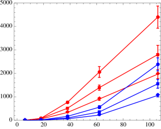
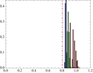
Figure 1: (a) CONF1-2D & 3D; (b) Convergence time for CONF1-3D for a varying number of cores and agents; (c) Empirical distribution of the objective over $1000$ random initializations of TWA for CONF1-3D.

In the supplementary movie we demonstrate the use of the landmark operators. First we show the use of these operators on six toy problems involving two agents and four landmark trajectories where we can use intuition to determine if the solutions found are good or bad. We solve these six scenarios using the ADMM with $100$ different random initializations to avoid local minima and reliably find very good solutions. With 1 core it always takes less than $3$ seconds to converge and typically less than $1$ second. We also solve a more complex problem involving $10$ agents and about $100$ landmarks whose solution is a ‘movie’ where the different robots act as pixels. With our landmark operators we do not have to pre-assign the robots to the pixels in each frame.

6 Conclusion

We introduced two novel proximal operators that allow the use of proximal algorithms to plan paths for agents in 3D, 4D, etc. and also to automatically assign waypoints to agents. The growing interest in coordinating large swarms of quadcopters in formation, for example, illustrates the importance of both extensions. For agents in 2D, our collision operator is substantially faster than its predecessor. In particular, it leads to an implementation of the velocity-obstacle local planning method that is faster than its implementation in both ? (?) and ? (?). The impact of our work goes beyond path planning. We are currently working on two other projects that use our results. One is related to visual tracking of multiple non-colliding large objects and the other is related to the optimal design of layouts, such as for electronic circuits. In the first, the speed of the new no-collision operator is crucial to achieve real-time performance and in the second we apply Lemma 3 to derive no-collision operators for non-circular objects.

The proximal algorithms used can get stuck in local minima, although empirically we find good solutions even for hard instances with very few or no random re-initializations. Future work might explore improving robustness, possibly by adding a simple method to start the TWA or the ADMM from a ‘good’ initial point. Finally, it would be valuable to implement wall-agent collision proximal operators that are more general than what we describe in Section 3, perhaps by exploring other methods to solve SIP problems.

Appendix for “Proximal Operators for Multi-Agent Path Planning”

Appendix A A comment on the impact of the assumption of piece-wise linear paths in practice

A direct application of the approach of ? (?) can result in very large accelerations at the break-points. It is however not hard to overcome this apparent limitation in practical applications. We now explain one way of doing it. First notice that by increasing the number of break-points we can obtain trajectories arbitrarily close to smooth trajectories with finite acceleration everywhere. Since in practice it is not efficient to work with a very large number of break-points, we can keep the number of break-points at a reasonable level and increase the effective radius of the robots. This would allow us to fit a polynomial through the break-points and obtain smooth trajectories that are never distant from the piece-wise linear paths by more than the difference between the true robots radii and their effective radii. Using this approach, we would obtain a set of non-colliding finite-acceleration trajectories. We can also impose specific maximum-acceleration constrains if, at the same time, we restrict the maximum permitted change of velocity at break-points using additional proximal operators.

Appendix B An illustration of the two kinds of blocks used by the ADMM/TWA

As explained in Section 2, the ADMM/TWA is an iterative scheme that alternates between (i) producing different estimates of the optimal value of the variables each function in the objective depends on and (ii) producing consensus values from the different estimates that pertain the same variable. The blocks that produce the estimates we call proximal operators and the blocks that produce consensus values we call consensus operators. The proximal operator blocks only receive messages from the consensus blocks (and send estimates back to them) and the consensus blocks only receive estimates from the proximal operators (and send consensus messages back to the proximal operators). Hence, the ADMM iteration scheme can be interpreted as messages passing back and forth along the edges of a bipartite graph.

We now illustrate this. Imagine that we want to compute non-colliding paths for two agents and that trajectories are parametrized by three break-points. In this case the optimization problem (1) has six variables, namely, $x_{1}(0),x_{1}(1),x_{1}(2)$ for agent $1$ and $x_{2}(0),x_{2}(1),x_{2}(2)$ for agent $2$. See Figure 2-(top).

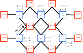
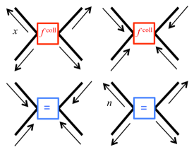
Figure 2: (Top) Variables in the problem; (Center) Graph of connections between proximal operators and consensus nodes; (Bottom) Proximal operators’ input and output values.

The ADMM has one consensus operator associated with the position of each agent at each break-point (blue blocks with ‘=’ sign on it) and has one proximal operator associated with each function in the objective (red blocks with function names on it). In our small example, we have two no-collision operators. One ensures there are no-collisions between the segment connecting $x_{1}(0)$ and $x_{1}(1)$ and the segment connecting $x_{2}(0)$ and $x_{2}(1)$. The other acts similarly on $x_{1}(1)$, $x_{1}(2)$, $x_{2}(1)$ and $x_{2}(2)$. We also have four velocity operators that penalize trajectories in which the path segments have large velocities. Finally, we have four position proximal operators that enforce agent $1$ and $2$ to start and finish their paths at specified locations. See Figure 2-(center).

The crucial part of implementing the ADMM or the TWA is the construction of the proximal operators. The proximal operators receive consensus messages $n$ from the consensus nodes and produce estimates for the values of the variables of the function associated to them. For example, at each iteration, the left-most no-collision proximal operator in Figure 2-(center) receives messages $n$ from the consensus nodes associated to the variables $x_{1}(0)$, $x_{1}(1)$, $x_{2}(0)$ and $x_{2}(1)$ and produces new estimates for their optimal value. The center-top consensus operator receives fours estimates for $x_{1}(1)$, from two no-collision proximal operators and two velocity proximal operators, and produces a single estimate its optimal value. See Figure 2-(bottom).

Appendix C A comment on our implementation of the TWA

Implementing the TWA requires computing proximal operators and specifying, at every iteration, what ? (?) calls the outgoing weights, $\overrightarrow{\rho}$, of each proximal operator. In the TWA there are also incoming weights, $\overleftarrow{\rho}$, which correspond to the $\rho$’s that appear in the definition of all our proximal operators, but their update scheme at every iteration is fixed (?, Section 4.1).

For the collision operator and landmark operator we introduce in this paper, we compute the outgoing weights using the same principle as in (?). Namely, if an operator maps a set of input variables $(n_{1},n_{2},...,n_{k})$ to a set of output variables $(x_{1},x_{2},...,x_{k})$ then, if $n_{i}\neq x_{i}$ we set $\overrightarrow{\rho}_{i}=1$ otherwise, when $n_{i}=x_{i}$, we set $\overrightarrow{\rho}_{i}=0$. In other words, if a variable is unchanged by the operators, the outgoing weight associated with it should be zero, otherwise it is $1$.

Appendix D More details about Remark 2

The next three points sketch why Remark 2 is true.

First, if the $\rho$’s are all positive, the objective function of problem (3) is strictly convex and we can add the constraint $\|(\underline{x},\underline{x}^{\prime},\overline{x},\overline{x}^{\prime})\|\leq M$, for $M$ large enough, without changing its minimum value. The new extended set of constraints amounts to the intersection of closed sets with a compact set and by the continuity of the objective function and the extreme value theorem it follows that the problem has a minimizer.

Second, problem (3) can be interpreted as resolving the following conflict. “Agent 1 wants to move from $\underline{n}$ at time $0$ to $\overline{n}$ at time $1$ and agent 2 wants to move from $\underline{n}^{\prime}$ at time $0$ to $\overline{n}^{\prime}$ at time $1$, however, if both move in a straight-line, they collide. How can we minimally perturb their initial and final reference positions so they they avoid collision?” If the vectors $(\underline{n},0)$, $(\underline{n}^{\prime},0)$, $(\overline{n},1)$,$(\overline{n}^{\prime},1)$ lie in the same three-dimensional plane there can be ambiguity on how to minimally perturb the agents’ initial and final positions: agent 1’s reference positions can either move ‘up’ and agent 2’s ‘down’ or agent 1’s reference positions ‘down’ and agent 2’s ‘up’ (‘up’ and ‘down’ relative to the plane defined by the vectors $(\underline{n},0)$, $(\underline{n}^{\prime},0)$, $(\overline{n},1)$,$(\overline{n}^{\prime},1)$). In numerical implementations however, it almost never happens that $(\underline{n},0)$, $(\underline{n}^{\prime},0)$, $(\overline{n},1)$,$(\overline{n}^{\prime},1)$ lie in the same plane and, in fact, this can be avoided by adding a very small amount of random noise to the $n$’s before solving problem (3).

Third, one can show from the continuity the objective function of problem (3) , the continuous-differentiability of $g(x,\alpha)=\|\alpha(\underline{x}-\underline{x}^{\prime})+(1-\alpha)(\overline{x}-\overline{x}^{\prime})\|^{2}-(r+r^{\prime})^{2}$ and the fact that the level sets of $g(x,\alpha)$ as a function of $x$ never have ‘flat’ sections that $h(\alpha)$ is a continuous function. Since $[0,1]$ is compact, it follows that there always exists an $\alpha^{*}$. Also, for the purpose of a numerical implementation, we can consider $\|\alpha^{*}(\underline{n}-\underline{n}^{\prime})+(1-\alpha^{*})(\overline{n}-\overline{n}^{\prime})\|\neq 0$. In fact, this can be avoided by adding a very small amount of random noise to the $n$’s before solving problem (4). Therefore, for practical purposes, we can consider that for each $\alpha^{*}$ there exists a unique minimizer to problem $\eqref{eq:coll_prox_op_single_alpha}$. Finally, a careful inspection of (5) shows that if there exists $\alpha$ such that $h(\alpha)>0$ then $\alpha^{*}$ is unique and if $h(\alpha)=0$ for all $\alpha$ then (6)-(9) always give $x=n$. In short, for the purpose of a numerical implementation, we always find a unique $x^{*}(\alpha^{*})$ and because, in practice, as argued in the two points above, problem (3) can be considered to have only one solution, it follows that this unique $x^{*}(\alpha^{*})$ is the unique minimizer of problem (3).

Appendix E Proof of Lemma 3

We need to consider two separate cases.

In the first case we assume that $x^{*}(\alpha^{*})$ is such that $g(x^{*}(\alpha^{*}),\alpha^{*})>0$. This implies that $x^{*}(\alpha^{*})$ is a minimizer of $\min_{x}f(x)$, which implies that $\min_{x:g(x,\alpha^{*})\geq 0}f(x)=\min_{x}f(x)$, which implies that $\min_{x:g(x,\alpha)\geq 0}f(x)\geq\min_{x}f(x)=\min_{x:g(x,\alpha^{*})\geq 0}f(x)=\max_{\alpha^{\prime}\in\mathcal{A}}\min_{x:g(x,\alpha^{\prime})\geq 0}f(x)\geq\min_{x:g(x,\alpha)\geq 0}f(x)$. In other words, $\min_{x:g(x,\alpha)\geq 0}f(x)=f(x^{*}(\alpha^{*}))$ for all $\alpha\in\mathcal{A}$. Since $f(x)$ has a unique minimizer we have that $x^{*}(\alpha^{*})$ must be feasible for the problem $\min_{x:g(x,\alpha)\geq 0}f(x)$, which implies that $g(x^{*}(\alpha^{*}),\alpha)\geq 0$ for all $\alpha\in\mathcal{A}$. In other words, $x^{*}(\alpha^{*})$ is feasible point of $\min_{x:g(x,\alpha)\geq 0\forall\alpha\in\mathcal{A}}f(x)$ and attains the smallest possible objective value, hence it minimizes it.

In the second case we assume that $g(x^{*}(\alpha^{*}),\alpha^{*})=0$. To finish the proof it suffices to show that $v\partial_{2}g(x^{*}(\alpha^{*}),\alpha^{*})\geq 0$ for all $v\in\mathbb{R}$ such that $\alpha^{*}+v\in\mathcal{A}$. To see this, we first notice that, if this is the case, then, for all $\alpha\in\mathcal{A}$, we have by convexity that $g(x^{*}(\alpha^{*}),\alpha)\geq g(x^{*}(\alpha^{*}),\alpha^{*})+(\alpha-\alpha^{*})\partial_{2}g(x^{*}(\alpha^{*}),\alpha^{*})=(\alpha-\alpha^{*})\partial_{2}g(x^{*}(\alpha^{*}),\alpha^{*})\geq 0$, which implies that $x^{*}(\alpha^{*})$ is a feasible point for the problem $\min_{x:g(x,\alpha)\geq 0,\forall\alpha\in\mathcal{A}}f(x)$. Secondly, we notice that $f(x^{*}(\alpha^{*}))\geq\min_{x:g(x,\alpha)\geq 0,\forall\alpha\in\mathcal{A}}f(x)\geq\max_{\alpha\in\mathcal{A}}\min_{x:g(x,\alpha)\geq 0}f(x)=f(x^{*}(\alpha^{*}))$. This implies that $x^{*}(\alpha^{*})$ minimizes $\min_{x:g(x,\alpha)\geq 0,\forall\alpha\in\mathcal{A}}f(x)$.

We now show that $v\partial_{2}g(x^{*}(\alpha^{*}),\alpha^{*})\geq 0$ for all $v\in\mathbb{R}$ such that $\alpha^{*}+v\in\mathcal{A}$.

First we notice that since $f$ is differentiable and $x^{*}(\alpha)$ exists and is differentiable at $x^{*}(\alpha^{*})$, then, by the chain rule, $h(\alpha)$ is differentiable at $\alpha^{*}$. In addition, we notice that if $\alpha^{*}$ maximizes $h$ then, if $v\in\mathbb{R}$ is such that $\alpha^{*}+v\in\mathcal{A}$, the directional derivative of $h$ in the direction of $v$ evaluated at $\alpha^{*}$ must be non-positive. In other words, $v\partial_{1}h(\alpha^{*})=v\partial_{1}f(x^{*}(\alpha^{*}))^{\dagger}\partial_{1}x^{*}(\alpha^{*})\leq 0$. Second, we notice that in a small neighborhood around $\alpha^{*}$, $x^{*}(\alpha)$ exists and is continuous (because $x^{*}(\alpha^{*})$ is differentiable) which, by the continuous-differentiability of $g$ and the fact that $\partial_{1}g(x^{*}(\alpha^{*}),\alpha^{*})\neq 0$, implies that $\partial_{1}g(x^{*}(\alpha),\alpha)\neq 0$ in this neighborhood. Therefore, in a small neighborhood around $\alpha^{*}$, the problem $\min_{x:g(x,\alpha)\geq 0}f(x)$ has a single inequality constraint and $\partial_{1}g(x^{*}(\alpha),\alpha)\neq 0$ which implies that $x^{*}(\alpha)$, which we are assuming exists in this neighborhood, is a feasible regular point and satisfies the first-order necessary optimality conditions (?)

$$\partial_{1}f(x^{*}(\alpha))+\lambda\partial_{1}g(x^{*}(\alpha),\alpha)=0,$$ (12)

$$\lambda g(x^{*}(\alpha),\alpha)=0,$$ (13)

$$g(x^{*}(\alpha),\alpha)\geq 0,$$ (14)

$$\lambda\leq 0.$$ (15)

Now, we take the directional derivative of (14) with respect to $\alpha$ in the direction $v$ evaluated at $(x^{*}(\alpha^{*}),\alpha^{*})$ and obtain

$$v\partial_{1}g(x^{*}(\alpha^{*}),\alpha^{*})^{\dagger}\partial_{1}x^{*}(\alpha^{*})+v\partial_{2}g(x^{*}(\alpha^{*}),\alpha^{*})\geq 0.$$ (16)

At the same time, by computing the inner product between (12) and $\partial_{1}x^{*}$ evaluated at $\alpha^{*}$ and multiplying by $v$ we obtain $v\partial_{1}f(x^{*}(\alpha^{*}))^{\dagger}\partial_{1}x^{*}(\alpha^{*})+\lambda v\partial_{1}g(x^{*}(\alpha^{*}),\alpha^{*})^{\dagger}\partial_{1}x^{*}(\alpha^{*})=0$. But we have already proved that $v\partial_{1}f(x^{*}(\alpha^{*}))^{\dagger}\partial_{1}x^{*}(\alpha^{*})\leq 0$ therefore $\lambda v\partial_{1}g(x^{*}(\alpha^{*}),\alpha^{*})^{\dagger}\partial_{1}x^{*}(\alpha^{*})\geq 0$. Now recall that we are assuming $g(x^{*}(\alpha^{*}),\alpha^{*})=0$ therefore, $\lambda<0$. It thus follows that $v\partial_{1}g(x^{*}(\alpha^{*}),\alpha^{*})^{\dagger}\partial_{1}x^{*}(\alpha^{*})\leq 0$ and from (16) we conclude that $v\partial_{2}g(x^{*}(\alpha^{*}),\alpha^{*})\geq 0$.

Appendix F Proof of Theorem 1

We first observe that the solutions to problem (3) and (4) remain the same if we replace $\|\alpha(\underline{x}-\underline{x}^{\prime})+(1-\alpha)(\overline{x}-\overline{x}^{\prime})\|\geq r+r^{\prime}$ by $\|\alpha(\underline{x}-\underline{x}^{\prime})+(1-\alpha)(\overline{x}-\overline{x}^{\prime})\|^{2}-(r+r^{\prime})^{2}\geq 0$. We prove the theorem with this replacement in mind.

We first prove the theorem assuming that we have proved that that expressions (5) to (9) hold when $\|\alpha(\underline{n}-\underline{n}^{\prime})+(1-\alpha)(\overline{n}-\overline{n}^{\prime})\|\neq 0$. This is then proved last.

To prove the theorem we consider two separate cases.

In the first case we consider $r+r^{\prime}\leq\min_{\alpha\in[0,1]}\|\alpha(\underline{n}-\underline{n}^{\prime})+(1-\alpha)(\overline{n}-\overline{n}^{\prime})\|$. This implies that the minimum of problem (3) is $0$ and, because the $\rho$’s are positive, there is a unique minimizer which equals $(\underline{n},\underline{n}^{\prime},\overline{n},\overline{n}^{\prime})$. In this case we also have $h(\alpha)=0$ for all $\alpha$, which implies that the solution of problem (4) is $x^{*}(\alpha)=n$ for all $\alpha$. Therefore, for any optimal $\alpha^{*}$ for which $\|\alpha^{*}(\underline{n}-\underline{n}^{\prime})+(1-\alpha^{*})(\overline{n}-\overline{n}^{\prime})\|\neq 0$, we have that the minimizer of problem (4) is equal to the unique solution of problem (3). Hence the theorem is true in this case.

Now we assume that $r+r^{\prime}>\min_{\alpha\in[0,1]}\|\alpha(\underline{n}-\underline{n}^{\prime})+(1-\alpha)(\overline{n}-\overline{n}^{\prime})\|$. This implies that there exists an $\alpha$ for which the right-hand-side of (5) is positive and for which $\|\alpha(\underline{n}-\underline{n}^{\prime})+(1-\alpha)(\overline{n}-\overline{n}^{\prime})\|\neq 0$. This implies that, there exists an $\alpha$ for which $h(\alpha)>0$. Therefore, for any optimal $\alpha^{*}$ it must the case that $h(\alpha^{*})>0$. If $\|\alpha^{*}(\underline{n}-\underline{n}^{\prime})+(1-\alpha^{*})(\overline{n}-\overline{n}^{\prime})\|\neq 0$ then (5) holds around a neighborhood of $\alpha^{*}$ and in this neighborhood $h(\alpha)>0$. Therefore, in this neighborhood $x^{*}(\alpha)$ exists, is unique, and is differentiable. Now we notice that the objective function of problem (3) is continuously-differentiable, and that $g(x,\alpha)\equiv\|\alpha(\underline{x}-\underline{x}^{\prime})+(1-\alpha)(\overline{x}-\overline{x}^{\prime})\|^{2}-(r+r^{\prime})^{2}$ is continuously-differentiable in $(x,\alpha)$ and convex in $\alpha$. If it is true that $\partial_{1}g(x^{*}(\alpha^{*}),\alpha^{*})\neq 0$ then we can apply Lemma 3 with $\mathcal{A}=[0,1]$ and conclude that $x^{*}(\alpha^{*})$ is also a solution of problem (3). Hence the theorem will be true in this case as well.

We now show that in this case, indeed, $\partial_{1}g(x^{*}(\alpha^{*}),\alpha^{*})\neq 0$. First we notice that $\partial_{1}g=(\partial_{\underline{x}}g,\partial_{\overline{x}}g,\partial_{\underline{x}^{\prime}}g,\partial_{\overline{x}^{\prime}}g)=2\|\alpha^{*}(\underline{x}^{*}-{\underline{x}^{*}}^{\prime})+(1-\alpha^{*})(\overline{x}^{*}-{\overline{x}^{*}}^{\prime})\|(\alpha^{*},1-\alpha^{*},-\alpha^{*},-1+\alpha^{*})$. We now recall that, as explain above, if $\|\alpha^{*}(\underline{n}-\underline{n}^{\prime})+(1-\alpha^{*})(\overline{n}-\overline{n}^{\prime})\|\neq 0$ then $h(\alpha^{*})>0$. Therefore, we conclude that $r+r^{\prime}=\|\alpha^{*}(\underline{x}^{*}-{\underline{x}^{*}}^{\prime})+(1-\alpha^{*})(\overline{x}^{*}-{\overline{x}^{*}}^{\prime})\|$ because otherwise $\|\alpha^{*}(\underline{x}^{*}-{\underline{x}^{*}}^{\prime})+(1-\alpha^{*})(\overline{x}^{*}-{\overline{x}^{*}}^{\prime})\|<r+r^{\prime}$ implies that the constraint of problem (4) for $\alpha=\alpha^{*}$ is inactive which implies that the solution must be $x=n$ with objective value $0$ which contradicts the fact that $h(\alpha^{*})>0$. Hence, $\partial_{1}g=(r+r^{\prime})(\alpha^{*},1-\alpha^{*},-\alpha^{*},-1+\alpha^{*})$, which is always non-zero, and proves that the theorem is true in this case as well.

Finally, we now prove that that expressions (5) to (9) hold when $\|\alpha(\underline{n}-\underline{n}^{\prime})+(1-\alpha)(\overline{n}-\overline{n}^{\prime})\|\neq 0$. This amounts to a relatively long calculus computation and is written in Appendix G.

Appendix G Computation of minimum value and minimizer of problem (4)

We do not solve problem (4) but instead solve the equivalent (more smooth) problem

$${\min_{\underline{x},\underline{x}^{\prime},\overline{x},\overline{x}^{\prime}}}\frac{\underline{\rho}}{2}\|\underline{x}-\underline{n}\|^{2}+\frac{\overline{\rho}}{2}\|\overline{x}-\overline{n}\|^{2}$$ (17)

$$+\frac{\underline{\rho}^{\prime}}{2}\|\underline{x}^{\prime}-\underline{n}^{\prime}\|^{2}+\frac{\overline{\rho}^{\prime}}{2}\|\overline{x}^{\prime}-\overline{n}^{\prime}\|^{2}$$

$$\text{ s.t. }\|\alpha(\underline{x}-\underline{x}^{\prime})+(1-\alpha)(\overline{x}-\overline{x}^{\prime})\|^{2}-(r+r^{\prime})^{2}\geq 0.$$

To begin, we notice that if

$$\|\alpha(\underline{n}-\underline{n}^{\prime})+(1-\alpha)(\overline{n}-\overline{n}^{\prime})\|>(r+r^{\prime})$$

then the constraint is inactive and the minimizer of (17) is $(\underline{n},\underline{n}^{\prime},\overline{n},\overline{n}^{\prime})$ with minimum value $0$. At the same time, if $\|\alpha(\underline{n}-\underline{n}^{\prime})+(1-\alpha)(\overline{n}-\overline{n}^{\prime})\|>(r+r^{\prime})$ we have that $h(\alpha)=0$ and the minimizer obtained from (6)-(9) is also $(\underline{n},\underline{n}^{\prime},\overline{n},\overline{n}^{\prime})$. Therefore, we only need to show that equations (5) and (6)-(9) hold in the case when the constraint is active, which corresponds to the case when $\|\alpha(\underline{n}-\underline{n}^{\prime})+(1-\alpha)(\overline{n}-\overline{n}^{\prime})\|\leq(r+r^{\prime})$.

To do so, we first introduce a few block variables (written in boldface) and express the above problem in a shorter form. Namely, we define ${\bf x}=(\underline{x},\underline{x}^{\prime},\overline{x},\overline{x}^{\prime})\in\mathbb{R}^{4\times d}$, ${\bf n}=(\underline{n},\underline{n}^{\prime},\overline{n},\overline{n}^{\prime})\in\mathbb{R}^{4\times d}$ and ${\boldsymbol{\alpha}}=(\alpha,-\alpha,(1-\alpha),-(1-\alpha))\in\mathbb{R}^{4}$ and $D=\text{diag}(\underline{\rho},\underline{\rho}^{\prime},\overline{\rho},\overline{\rho}^{\prime})\in\mathbb{R}^{4\times 4}$, and, rewrite (17) as

$$\begin{aligned} &&{\min_{\bf x}}\;\;\;&\frac{1}{2}\text{tr}\{({\bf x-n})^{\dagger}D({\bf x-n})\}\\ &&\text{s.t.}\;\;\;&\|{\boldsymbol{\alpha}}^{\dagger}{\bf x}\|^{2}-(r+r^{\prime})^{2}\geq 0.\end{aligned}$$ (18)

Then we notice that it is necessary that the solutions to this problem are among the points that satisfy the KKT conditions. Namely, those points that satisfy

$$D({\bf x-n})+2{\boldsymbol{\alpha}}v=0$$ (19)

$$v=\lambda({\boldsymbol{\alpha}}^{\dagger}{\bf x})$$ (20)

$$\|v\|/|\lambda=r+r^{\prime}$$ (21)

where $\lambda\neq 0$ is the Lagrange multiplier associated to the problem’s constraint and is non-zero because we are assuming the constraint is active. In the rest of the proof we show that there are only two points that satisfy the KKT conditions and show that, between them, the one that corresponds to the global optimum satisfies (5) and (6)-(9).

We first write the two equations even more compactly as

$$\left(\begin{array}[]{cc}\frac{1}{2}D&{\boldsymbol{\alpha}}\\ {\boldsymbol{\alpha}}^{\dagger}&-1/\lambda\end{array}\right)\left(\begin{array}[]{c}{\bf x}\\ v\end{array}\right)=\left(\begin{array}[]{c}\frac{1}{2}D{\bf n}\\ 0\end{array}\right).$$ (22)

We claim that, if $1+2\lambda{\boldsymbol{\alpha}}^{\dagger}D^{-1}{\boldsymbol{\alpha}}\neq 0$, the inverse of the block matrix

$$\left(\begin{array}[]{cc}\frac{1}{2}D&{\boldsymbol{\alpha}}\\ {\boldsymbol{\alpha}}^{\dagger}&-1/\lambda\end{array}\right)$$ (23)

is

$$\left(\begin{array}[]{cc}2\left(D^{-1}-\frac{2D^{-1}\lambda{\boldsymbol{\alpha}}{\boldsymbol{\alpha}}^{\dagger}D^{-1}}{1+2\lambda{\boldsymbol{\alpha}}^{\dagger}D^{-1}{\boldsymbol{\alpha}}}\right)&\frac{2\lambda D^{-1}{\boldsymbol{\alpha}}}{1+2\lambda{\boldsymbol{\alpha}}^{\dagger}D^{-1}{\boldsymbol{\alpha}}}\\ \frac{2\lambda{\boldsymbol{\alpha}}^{\dagger}D^{-1}}{1+2\lambda{\boldsymbol{\alpha}}^{\dagger}D^{-1}{\boldsymbol{\alpha}}}&\frac{-\lambda}{1+2\lambda{\boldsymbol{\alpha}}^{\dagger}D^{-1}{\boldsymbol{\alpha}}}\end{array}\right).$$ (24)

To prove this we could use the formula for the inverse of a block matrix. Instead, and much more simply, we simply compute the product of (24) and (23) and show it equals the identify. It is immediate to see that the block diagonal entries of the resulting product are indeed identity matrices. Since both matrices are symmetric, all that is left to check is that one of the non-diagonal block entries is zero. Indeed,

$$({\boldsymbol{\alpha}}^{\dagger})\left(2\left(D^{-1}-\frac{2D^{-1}\lambda{\boldsymbol{\alpha}}{\boldsymbol{\alpha}}^{\dagger}D^{-1}}{1+2\lambda{\boldsymbol{\alpha}}^{\dagger}D^{-1}{\boldsymbol{\alpha}}}\right)\right)$$

$$+(-1/\lambda)\left(\frac{2\lambda{\boldsymbol{\alpha}}^{\dagger}D^{-1}}{1+2\lambda{\boldsymbol{\alpha}}^{\dagger}D^{-1}{\boldsymbol{\alpha}}}\right)$$

$$=\frac{2{\boldsymbol{\alpha}}^{\dagger}D^{-1}(1+2\lambda{\boldsymbol{\alpha}}^{\dagger}D^{-1}{\boldsymbol{\alpha}})-4{\boldsymbol{\alpha}}^{\dagger}D^{-1}\lambda{\boldsymbol{\alpha}}{\boldsymbol{\alpha}}^{\dagger}D^{-1}-2{\boldsymbol{\alpha}}^{\dagger}D^{-1}}{1+2\lambda{\boldsymbol{\alpha}}^{\dagger}D^{-1}{\boldsymbol{\alpha}}}$$

$$=\frac{4\lambda{\boldsymbol{\alpha}}^{\dagger}D^{-1}{\boldsymbol{\alpha}}^{\dagger}D^{-1}{\boldsymbol{\alpha}}-4{\boldsymbol{\alpha}}^{\dagger}D^{-1}\lambda{\boldsymbol{\alpha}}{\boldsymbol{\alpha}}^{\dagger}D^{-1}}{1+2\lambda{\boldsymbol{\alpha}}^{\dagger}D^{-1}{\boldsymbol{\alpha}}}$$

$$=\frac{({\boldsymbol{\alpha}}^{\dagger}D^{-1}{\boldsymbol{\alpha}})(4\lambda{\boldsymbol{\alpha}}^{\dagger}D^{-1}-4\lambda{\boldsymbol{\alpha}}^{\dagger}D^{-1})}{1+2\lambda{\boldsymbol{\alpha}}^{\dagger}D^{-1}{\boldsymbol{\alpha}}}=0.$$

We now solve the linear system (22) by multiplying both sides by the inverse matrix (24) and, we conclude that

$$v=\frac{2\lambda{\boldsymbol{\alpha}}^{\dagger}D^{-1}}{1+2\lambda{\boldsymbol{\alpha}}^{\dagger}D^{-1}{\boldsymbol{\alpha}}}\left(\frac{1}{2}D{\bf n}\right)=\frac{\lambda{\boldsymbol{\alpha}}^{\dagger}{\bf n}}{1+2\lambda{\boldsymbol{\alpha}}^{\dagger}D^{-1}{\boldsymbol{\alpha}}},$$ (25)

$${\bf x}=2\left(D^{-1}-\frac{2D^{-1}\lambda{\boldsymbol{\alpha}}{\boldsymbol{\alpha}}^{\dagger}D^{-1}}{1+2\lambda{\boldsymbol{\alpha}}^{\dagger}D^{-1}{\boldsymbol{\alpha}}}\right)\left(\frac{1}{2}D{\bf n}\right)$$

$$={\bf n}-\frac{2D^{-1}\lambda{\boldsymbol{\alpha}}{\boldsymbol{\alpha}}^{\dagger}{\bf n}}{1+2\lambda{\boldsymbol{\alpha}}^{\dagger}D^{-1}{\boldsymbol{\alpha}}}.$$ (26)

Using equation (26) we can express the objective value of (18) as

$$\frac{1}{2}\text{tr}\{({\bf x-n})^{\dagger}D({\bf x-n})\}$$

$$=\frac{\text{tr}\{{\bf n}^{\dagger}{\boldsymbol{\alpha}}{\boldsymbol{\alpha}}^{\dagger}\lambda D^{-1}(-2)D(-2)D^{-1}\lambda{\boldsymbol{\alpha}}{\boldsymbol{\alpha}}^{\dagger}{\bf n}\}}{2(1+2\lambda{\boldsymbol{\alpha}}^{\dagger}D^{-1}{\boldsymbol{\alpha}})^{2}}$$

$$=\frac{\text{tr}\{{\bf n}^{\dagger}{\boldsymbol{\alpha}}{\boldsymbol{\alpha}}^{\dagger}{\bf n}\}4\lambda^{2}({\boldsymbol{\alpha}}^{\dagger}D^{-1}{\boldsymbol{\alpha}})}{2(1+2\lambda{\boldsymbol{\alpha}}^{\dagger}D^{-1}{\boldsymbol{\alpha}})^{2}}$$

$$=\frac{2\lambda^{2}\|{\boldsymbol{\alpha}}^{\dagger}{\bf n}\|^{2}({\boldsymbol{\alpha}}^{\dagger}D^{-1}{\boldsymbol{\alpha}})}{(1+2\lambda{\boldsymbol{\alpha}}^{\dagger}D^{-1}{\boldsymbol{\alpha}})^{2}}=2\|v\|^{2}({\boldsymbol{\alpha}}^{\dagger}D^{-1}{\boldsymbol{\alpha}}),$$

where in the last equality we made use of (25). We now recall that from the third equation in the KKT conditions we have that $\|v\|/\lambda=r+r^{\prime}$ and so we conclude that

$$\lambda=\frac{1}{2({\boldsymbol{\alpha}}^{\dagger}D^{-1}{\boldsymbol{\alpha}})}\left(-1\pm\frac{\|{\boldsymbol{\alpha}}^{\dagger}{\bf n}\|}{r+r^{\prime}}\right),$$ (27)

and therefore,

$$\frac{1}{2}\text{tr}\{({\bf x-n})^{\dagger}D({\bf x-n})\}$$

$$=2(r+r^{\prime})^{2}\frac{1}{4({\boldsymbol{\alpha}}^{\dagger}D^{-1}{\boldsymbol{\alpha}})^{2}}\left(-1\pm\frac{\|{\boldsymbol{\alpha}}^{\dagger}{\bf n}\|}{r+r^{\prime}}\right)^{2}({\boldsymbol{\alpha}}^{\dagger}D^{-1}{\boldsymbol{\alpha}})$$

$$=\frac{(r+r^{\prime}\pm\|{\boldsymbol{\alpha}}^{\dagger}{\bf n}\|)^{2}}{2({\boldsymbol{\alpha}}^{\dagger}D^{-1}{\boldsymbol{\alpha}})}.$$ (28)

Since we are seeking the global minimum, and since we are assuming that $\|{\boldsymbol{\alpha}}^{\dagger}{\bf n}\|=\|\alpha(\underline{n}-\underline{n}^{\prime})+(1-\alpha)(\overline{n}-\overline{n}^{\prime})\|\leq(r+r^{\prime})$ and hence the constraint is active, we conclude that

$$\frac{1}{2}\text{tr}\{({x^{*}(\alpha)-n})^{\dagger}D({x^{*}(\alpha)-n})\}$$

$$=\frac{(r+r^{\prime}-\|{\boldsymbol{\alpha}}^{\dagger}{\bf n}\|)^{2}}{2({\boldsymbol{\alpha}}^{\dagger}D^{-1}{\boldsymbol{\alpha}})}=\frac{1}{2}(h(\alpha))^{2}.$$ (29)

Above we have used the fact that ${\boldsymbol{\alpha}}^{\dagger}{\bf n}=\alpha\Delta\underline{n}+(1-\alpha)\Delta\overline{n}$ and that ${\boldsymbol{\alpha}}^{\dagger}D^{-1}{\boldsymbol{\alpha}}=\alpha^{2}/\utilde{\rho}+(1-\alpha)^{2}/\tilde{\rho}$. This proves that (5) is valid when $\|{\boldsymbol{\alpha}}^{\dagger}{\bf n}\|=\|\alpha(\underline{n}-\underline{n}^{\prime})+(1-\alpha)(\overline{n}-\overline{n}^{\prime})\|\leq(r+r^{\prime})$ as long as $1+2\lambda{\boldsymbol{\alpha}}^{\dagger}D^{-1}{\boldsymbol{\alpha}}=\|{\boldsymbol{\alpha}}^{\dagger}{\bf n}\|/(r+r^{\prime})\neq 0$. Recall that we have already proved that (5) holds when when $\|{\boldsymbol{\alpha}}^{\dagger}{\bf n}\|=\|\alpha(\underline{n}-\underline{n}^{\prime})+(1-\alpha)(\overline{n}-\overline{n}^{\prime})\|>(r+r^{\prime})$.

To finish the proof we now prove the validity of (6)-(9) when $\|{\boldsymbol{\alpha}}^{\dagger}{\bf n}\|=\|\alpha(\underline{n}-\underline{n}^{\prime})+(1-\alpha)(\overline{n}-\overline{n}^{\prime})\|>(r+r^{\prime})$. Recall that we have already proved their validity when $\|{\boldsymbol{\alpha}}^{\dagger}{\bf n}\|=\|\alpha(\underline{n}-\underline{n}^{\prime})+(1-\alpha)(\overline{n}-\overline{n}^{\prime})\|\leq(r+r^{\prime})$. Now notice that, when $\|{\boldsymbol{\alpha}}^{\dagger}{\bf n}\|=\|\alpha(\underline{n}-\underline{n}^{\prime})+(1-\alpha)(\overline{n}-\overline{n}^{\prime})\|>(r+r^{\prime})$, we can write,

$$\lambda=\frac{1}{2({\boldsymbol{\alpha}}^{\dagger}D^{-1}{\boldsymbol{\alpha}})}\left(-1+\frac{\|{\boldsymbol{\alpha}}^{\dagger}{\bf n}\|}{r+r^{\prime}}\right)$$

$$=-\frac{h(\alpha)}{2(r+r^{\prime})\sqrt{{\boldsymbol{\alpha}}^{\dagger}D^{-1}{\boldsymbol{\alpha}}}}.$$ (30)

If we define $\gamma=\frac{2\lambda}{1+2\lambda{\boldsymbol{\alpha}}^{\dagger}D^{-1}{\boldsymbol{\alpha}}}$, we can write the following expression for ${x}^{*}(\alpha)$

$${x}^{*}(\alpha)={\bf n}-\gamma D^{-1}{\boldsymbol{\alpha}}{\boldsymbol{\alpha}}^{\dagger}{\bf n},$$ (31)

which holds if $\|{\boldsymbol{\alpha}}^{\dagger}{\bf n}\|=\|\alpha(\underline{n}-\underline{n}^{\prime})+(1-\alpha)(\overline{n}-\overline{n}^{\prime})\|\neq 0$. With a little bit of algebra one can see that this is exactly the same expression as (6)-(9) and finish the proof.

References

- [2012a] Alonso-Mora, J.; Breitenmoser, A.; Beardsley, P.; and Siegwart, R. 2012a. Reciprocal collision avoidance for multiple car-like robots. In Robotics and Automation, IEEE Intern. Conf. on, 360–366.
- [2012b] Alonso-Mora, J.; Breitenmoser, A.; Rufli, M.; Siegwart, R.; and Beardsley, P. 2012b. Image and animation display with multiple mobile robots. The International Journal of Robotics Research 31(6):753–773.
- [2012c] Alonso-Mora, J.; Schoch, M.; Breitenmoser, A.; Siegwart, R.; and Beardsley, P. 2012c. Object and animation display with multiple aerial vehicles. In Intelligent Robots and Systems, IEEE/RSJ Intern. Conf. on, 1078–1083. IEEE.
- [2013] Alonso-Mora, J.; Rufli, M.; Siegwart, R.; and Beardsley, P. 2013. Collision avoidance for multiple agents with joint utility maximization. In Robotics and Automation, IEEE Intern. Conf. on, 2833–2838.
- [2001] Andreev, A.; Pavisic, I.; and Raspopovic, P. 2001. Metal layer assignment. US Patent 6,182,272.
- [2012] Augugliaro, F.; Schoellig, A. P.; and D’Andrea, R. 2012. Generation of collision-free trajectories for a quadrocopter fleet: A sequential convex programming approach. In Intelligent Robots and Systems, IEEE/RSJ Intern. Conf. on, 1917–1922.
- [2003] Bahceci, E.; Soysal, O.; and Sahin, E. 2003. A review: Pattern formation and adaptation in multi-robot systems. Robotics Institute, Carnegie Mellon University, Pittsburgh, PA, Tech. Rep. CMU-RI-TR-03-43.
- [2013] Bento, J.; Derbinsky, N.; Alonso-Mora, J.; and Yedidia, J. S. 2013. A message-passing algorithm for multi-agent trajectory planning. In Advances in Neural Information Processing Systems, 521–529.
- [1988] Bertsekas, D. P. 1988. The auction algorithm: A distributed relaxation method for the assignment problem. Annals of Operations Research 14(1):105–123.
- [1999] Bertsekas, D. P. 1999. Nonlinear programming.
- [2011] Boyd, S.; Parikh, N.; Chu, E.; Peleato, B.; and Eckstein, J. 2011. Distributed optimization and statistical learning via the alternating direction method of multipliers. Foundations and Trends in Machine Learning 3(1):1–122.
- [2013] Derbinsky, N.; Bento, J.; Elser, V.; and Yedidia, J. S. 2013. An improved three-weight message-passing algorithm. arXiv:1305.1961 [cs.AI].
- [1998] Fiorini, P., and Shiller, Z. 1998. Motion planning in dynamic environments using velocity obstacles. The International Journal of Robotics Research 17(7):760–772.
- [1988] Goldberg, A. V., and Tarjan, R. E. 1988. A new approach to the maximum-flow problem. Journal of the ACM (JACM) 35(4):921–940.
- [1984] Hopcroft, J. E.; Schwartz, J. T.; and Sharir, M. 1984. On the complexity of motion planning for multiple independent objects; pspace-hardness of the ”warehouseman’s problem”. The International Journal of Robotics Research 3(4):76–88.
- [2010] Karaman, S., and Frazzoli, E. 2010. Incremental sampling-based algorithms for optimal motion planning. arXiv:1005.0416 [cs.RO].
- [1994] Kavraki, L., and Latombe, J.-C. 1994. Randomized preprocessing of configuration for fast path planning. In Robotics and Automation, IEEE Intern. Conf. on, 2138–2145. IEEE.
- [1996] Kavraki, L. E.; Svestka, P.; Latombe, J.-C.; and Overmars, M. H. 1996. Probabilistic roadmaps for path planning in high-dimensional configuration spaces. Robotics and Automation, IEEE Transactions on 12(4):566–580.
- [2002] Kuffner, J.; Nishiwaki, K.; Kagami, S.; Kuniyoshi, Y.; Inaba, M.; and Inoue, H. 2002. Self-collision detection and prevention for humanoid robots. In Robotics and Automation, 2002. Proceedings. ICRA’02. IEEE International Conference on, volume 3, 2265–2270. IEEE.
- [1955] Kuhn, H. W. 1955. The hungarian method for the assignment problem. Naval Research Logistics Quarterly 2(1-2):83–97.
- [2001] LaValle, S. M., and Kuffner, J. J. 2001. Randomized kinodynamic planning. The International Journal of Robotics Research 20(5):378–400.
- [2012] Mellinger, D.; Kushleyev, A.; and Kumar, V. 2012. Mixed-integer quadratic program trajectory generation for heterogeneous quadrotor teams. In Robotics and Automation, IEEE Intern. Conf. on, 477–483. IEEE.
- [2008] Michael, N.; Zavlanos, M. M.; Kumar, V.; and Pappas, G. J. 2008. Distributed multi-robot task assignment and formation control. In Robotics and Automation, IEEE Intern. Conf. on, 128–133. IEEE.
- [2013] Parikh, N., and Boyd, S. 2013. Proximal algorithms. Foundations and Trends in Optimization 1(3):123–231.
- [2010] Ratti, C., and Frazzoli, E. 2010. Flyfire.
- [1979] Reif, J. H. 1979. Complexity of the mover’s problem and generalizations. In IEEE Annual Symposium on Foundations of Computer Science, 421–427.
- [2013] Sharon, G.; Stern, R.; Goldenberg, M.; and Felner, A. 2013. The increasing cost tree search for optimal multi-agent pathfinding. Artificial Intelligence 195:470–495.
- [] Standley, T., and Korf, R. Complete algorithms for cooperative pathfinding problems.
- [2012] Stein, O. 2012. How to solve a semi-infinite optimization problem. European Journal of Operational Research 223(2):312–320.
- [2014] Udell, M., and Boyd, S. 2014. Bounding duality gap for problems with separable objective.
- [1988] Witkin, A., and Kass, M. 1988. Spacetime constraints. In ACM Siggraph Computer Graphics, volume 22, 159–168. ACM.