Heterogeneous Tensor Decomposition for Clustering via Manifold Optimization
Abstract
Tensors or multiarray data are generalizations of matrices. Tensor clustering has become a very important research topic due to the intrinsically rich structures in real-world multiarray datasets. Subspace clustering based on vectorizing multiarray data has been extensively researched. However, vectorization of tensorial data does not exploit complete structure information. In this paper, we propose a subspace clustering algorithm without adopting any vectorization process. Our approach is based on a novel heterogeneous Tucker decomposition model. In contrast to existing techniques, we propose a new clustering algorithm that alternates between different modes of the proposed heterogeneous tensor model. All but the last mode have closed-form updates. Updating the last mode reduces to optimizing over the so-called multinomial manifold, for which we investigate second order Riemannian geometry and propose a trust-region algorithm. Numerical experiments show that our proposed algorithm compete effectively with state-of-the-art clustering algorithms that are based on tensor factorization.
Index Terms:
Tensor Clustering, Tucker Decomposition, Heterogeneous Tensor Decomposition, Manifold Optimization, Multinomial Manifold1 Introduction
In the last two decades, the advance of modern sensing, networking, communication and storage technologies have paved the way for the availability of multidimensional data with high dimensionality. For example, remote sensing is producing massive multidimensional data that need to be carefully analyzed. One of the characteristics of these gigantic datasets is that they often have a large amount of redundancies. This motivates the development of a low-dimensional representation that best assists a range of learning tasks in order to avoid the so-called “curse of dimensionality” [1]. Many data processing tasks involve manipulating multi-dimensional objects. For example, video data [2] can be regarded as an object of pixel location in two dimensions plus one dimension in time. Similar representation can be seen in manipulating remote sensing data [3]. In analyzing personalized webpages, the data is usually represented as a third order dataset with three dimensional modes of users, query words and webpages, respectively [4]. In document clustering, one presents the dataset in a three-way format of authors, terms and times [5, 6].
The multi-dimensional data are known as tensors [7, 8], where data elements are addressed by more than two indices. An -order tensor is an element of the tensor product of vector spaces. A 2D matrix is an example of the 2nd-order tensor. Similarly, hyperspectral imagery [9] is naturally a three-dimensional (3D) data cube containing both spatial and spectral dimensions. Simultaneously considering both spectral and spatial structures of hyperspectral data in clustering or classification lead to superior results, e.g., in [27]. To this end, we prefer treating, e.g., a 3D cube as a whole. In order to circumvent the issue of high dimensionality, a strategy is to compress the data while capturing the dominant trends or to find the most suitable “sparse” representation of the data.
Data clustering is one of the widely used data mining techniques [10]. Many clustering methods consider each data as a high dimensional mathematical vector A typical way is to pre-process those high dimensional vectors with dimensionality reduction techniques such as principal component analysis (PCA) [11]. For dealing with tensorial data, a conventional step is to first vectorize them before any analysis is applied. For example, this procedure is practiced to convert image data, a 2nd-order tensor, into vectors for processing. Not surprisingly, this strategy breaks higher order dependencies that may be present in the data. Recently, new approaches that are capable of directly processing structural information of tensorial data have been proposed, e.g., tensorial data structure is exploited in computer vision applications [13, 14] and machine learning [15, 16].
Tensorial data have a large amount of redundancies. It is desired to have a mechanism to reduce such redundancies for the sake of efficient application of learning algorithms. We use the general term dimensionality reduction to describe such techniques or models. There exist various tensor decomposition models, amongst which the CANDECOMP (canonical decomposition)/PARAFAC (parallel factors) or in short CP decomposition [17] and the Tucker decomposition are two fundamental models for tensor decomposition (refer to the survey paper [8] for details). It should be noted that the CP decomposition is a special case of the Tucker decomposition [8], where the factor matrices have same number of columns and the core tensor is superdiagonal, which means that every mode of the tensor is of the same size and its elements remain constant under any permutation of the indices. Many other decomposition algorithms/models can be viewed as special formats of the CP and Tucker decomposition. For example, the higher order SVD algorithm (HOSVD) [18], an extension of the classical SVD, is a special case of the general Tucker decomposition of a tensor in which the core tensor is of the same dimension as the tensor to be decomposed and all the mode matrices have orthonormal columns. Similarly, the classical PCA has several extensions for tensorial data. The generalized tensor PCA (GND-PCA) seeks a shared Tucker decomposition for all the given tensors in which the core tensors are different but the matrix factors along each mode are orthogonal. This decomposition procedure is also called the higher-order orthogonal iteration (HOOI) algorithm in [19].
In applications where data are non-negative such as images, the non-negative matrix factorization (NFM) has proven to be a successful approach for detecting essential features in the data [20]. Several efficient algorithms have been proposed [21, 22]. Recently, NFM has been extended to non-negative tensor factorization (NTF) and has been investigated in [15, 23, 24, 25, 26].
Another trend in tensor decomposition research is to introduce more structures in the decomposition model itself. Recently, Zhang et al. [27] considered Tri-ONTD (Tri-factor orthogonal non-negative tensor decomposition), a new tensor decomposition model. The fundamental aim of this model is to discover common characteristics of a series of matrix data. A straightforward application of Tri-ONTD is to identify cluster structures of a dataset. The core idea behind this model is based on the centroid-based clustering algorithms such as the k-means algorithm. The idea of introducing new structures in tensor decomposition can also be seen in [28] in the context of image representation.
Often tensor clustering tasks are formulated as optimization problems on specific tensor decomposition models [29, 30, 31, 32]. For example, when imposing some specific constraints, like orthogonality in the HOOI algorithm [19], the resulting problems reduce to optimization over matrix manifolds [33]. In the case of the HOOI algorithm for the HOSVD decomposition, the resulting optimization problem is on the Stiefel manifold [33, Section 3.3]). While the optimization problem in HOSVD admits a closed-form solution under the least squared error criterion, computing a closed-form solution is not possible for the tensor clustering problem that we consider in this paper. Most existing algorithms avoid this issue by reformulating it into an optimization problem over the “flat” Euclidean space with some treatment, e.g., by introducing a regularization term.
Recent years have witnessed significant development of Riemannian optimization algorithms on matrix manifolds such as the Stiefel manifold, the Grassmann manifold, and the manifold of positive definite matrices [33, 35, 36]. The Riemannian optimization framework endows a matrix manifold constraint with a Riemannian manifold structure. Conceptually, it translates a constrained optimization problem into an unconstrained optimization problem on a Riemannian manifold. Since the Riemannian optimization framework is directly based on nonlinear manifolds, one can eliminate those constraints such as orthogonality to obtain an unconstrained optimization problem that, by construction, will only use feasible points. The recent successful applications of the Riemannian optimization framework in machine learning, computer vision and data mining, include low rank optimization [34, 35, 36], estimation [37], Riemannian dictionary learning [38, 39], and computer vision tasks [40], to name a few.
In this paper, we propose a novel subspace clustering algorithm that exploits the tensorial structure of data. To this end, we introduce a new heterogeneous Tucker decomposition model. The proposed clustering algorithm alternates between different modes of the proposed heterogeneous tensor model. All but the last mode have closed-form updates. Updating the last mode reduces to optimizing over the multinomial manifold, defined in Section 3, for which we investigate second order Riemannian geometry and propose a trust-region algorithm. The multinomial manifold is given a Riemannian manifold structure by endowing it with the Fisher information metric [46, 44]. The Fisher information metric gives the multimonial manifold a differentiable structure, i.e., it ensures that the boundary is “scaled” to infinity.
The contribution of this paper is twofold. First, we propose a heterogeneous Tucker decomposition model for tensor clustering. Second, we investigate the Riemannian geometry of the multinomial manifold and apply the Riemannian trust-region algorithm to the resulting nonlinear clustering problem over the multinomial manifold.
The paper is organized as follows. We introduce the notations for tensor representation and operations used in this paper in Section 2.1. Section 2.2 introduces the clustering scheme based on the proposed heterogeneous Tucker decomposition model. The associated optimization problems are discussed in Section 2.3. Section 3 explores the Riemannian geometry for the multinomial manifold and develops all the necessary optimization-related ingredients. Section 4 presents the algorithm procedure for the tensor clustering including the proposed Riemannian trust-region algorithm. Section 5 shows numerical experimental results on both synthetic tensorial data and real-world datasets. Finally Section 6 concludes the paper.
2 Heterogeneous Tucker decomposition model for clustering
In this section, starting with notation for tensors, we motivate the work, and finally propose the new heterogeneous Tucker decomposition model for clustering.
2.1 Tensor Notation and Operations
In the sequel, we follow the convention used in [8] to denote 1D vector by lowercase boldface symbols like , 2D matrix by uppercase boldface symbols like and general tensors by calligraphy symbols like .
Let be an -order tensor with as the th element. The -mode product of an -order tensor with a matrix is denoted by . The result is an -order tensor of dimension . Element wise, the -mode product is expressed as
Given an -order tensor , we seek a Tucker model, as defined below, to approximate the tensor as
| (1) |
where is an -order tensor of dimension with , called the core tensor, and is the matrix applied along mode-. In this decomposition, the core tensor is interpreted as a lower dimensional representation of the tensor . The Tucker decomposition is a form of higher-order PCA [41], where all the factor matrices are shared by a group of given tensors.
2.2 Heterogeneous Tucker Decomposition Model
Most Tucker decomposition models are of a homogeneous nature, by which we mean that all the factor matrices satisfy the same constraint. For example, in the classical HOSVD [8], all the factor matrices are required to be orthogonal, i.e., (denoted by for simplicity). In the nonnegative Tucker decomposition model [24, 25], all the factors are matrices with nonnegative entries, i.e., .
However, the requirement for homogeneous factors is not preferred in many cases. Especially, when the factor matrices in different modes have different interpretations. For example, consider the problem of clustering a set of images (2-order tensors). We can stack all the images onto a 3-order tensor, where the third mode corresponds to the number of images. For clustering the images, it is of interest to decompose the entire 3-order tensor in a way that, along the third mode, each image is represented by several cluster representatives, as done in fuzzy k-means algorithms. This can be achieved by ensuring that the last mode factor matrix, i.e., is nonnegative and the row sum of is to mimic the cluster probability of an image.
In general, we suppose that we are given a set of -order tensors, denoted by and we want cluster them into clusters. This can be done by projecting the tensors along all the first modes, then cluster them. To this end, we stack all the -order tensors along the mode, so that we have an -order tensor in a way that each slice of , along the last mode, is one of -order tensors (). Following the general notation in Section 2.1, we have .
Our proposed model is defined by the optimization problem
| (2) |
with
where is a column vector of all ones, are matrices whose columns are orthogonal, denotes the Frobenius norm, and is nonnegative and the sum of each row is . In (2), the dimension of in mode is .
If each of the slices of is interpreted as cluster centroids in the projected space , then the rows of has the interpretation of cluster indicators.
Given this heterogeneous Tucker decomposition model that is specifically aimed for clustering, we have a new type of matrix manifold, that is the cartesian product of the Stiefel manifolds, corresponding to the constraints and the the multinomial manifold that corresponds to . It should be noted that the problem (2) needs two different treatments in terms of optimizing their factor matrices, i.e., for the first orthogonal matrices and the tensor clustering indicator matrix , respectively. In the following we formulate these optimization problems.
2.3 Optimization
To reduce the number of optimization variables in problem (2), let us optimize the core tensor when all the factor matrices are fixed to their current values. This becomes a least-squares problem. It is straightforward to prove that the solution is given by [8]
| (3) |
where we have used the orthogonality of (). It should be noted that is column full rank.
It should be emphasized that the function is smooth in the variables and the constraints are separable. This motivates to consider an alternating optimization scheme for (4), where we maximize (4) with respect to one variable while fixing others. This procedure is cyclically repeated.
Let . If all but () are fixed, then is optimized by solving an eigenvector problem. Specifically, consider updating () while all the others being fixed. Denote
Subsequently, (4) can be rewritten as, after mode- matricization,
| (5) |
where is the -mode matricization of tensor . The problem (5) has a closed-form solution given by, letting ,
| (6) |
where extracts the orthogonal factor of the polar decomposition of its argument and is computed as , where is the thin singular value decomposition of .
As discussed in Section 2.2, the nonnegativity constraint on is specifically introduced for clustering, leading to the optimization problem
| (7) |
where
with as the -mode matricization of and is the Kronecker product of matrices.
Problem (7) is a nonlinear optimization problem over the constraint , called the multinomial manifold, where is the vector of all ones. An efficient numerical algorithm is needed. To this end, we propose an a trust-region algorithm in Section 4.1 based on the Riemannian structure of the multinomial manifold that is discussed in Section 3.
3 The multinomial manifold
For the concepts of general abstract manifolds, we refer readers to the textbook [43]. Each row of is a discrete probability distribution which describes the membership over the tensor centroids. All the discrete probability distributions make up the multinomial manifold (also called a simplex) defined by
It should be noted that the nonnegativity constraint is replaced with strict positivity to ensure that the set is differentiable. A possible use of the multinomial manifold is in proposing a classifier with kernels, e.g., in [44, 45, 46]. For the purpose of solving the optimization problem (7), we investigate the product manifold of multiple multinomial manifolds, still called the multinomial manifold, defined as
Despite the use of the Fisher information metric on the multinomial manifold in [44, 46], to the best of our knowledge, the derivation of the Riemannian gradient and the Riemannian Hessian of a smooth objective function is new. The computations are shown in the subsequent sections.
3.1 The Submanifold Structure
Let us represent an element of with the notation which is the matrix representation of size . It is straightforward to show that the tangent space at is given by
where is a column vector of all ones and is a column vector of all zeros.
It should also be noted that, we can characterize the manifold as an embedded Riemannian submanifold of the Euclidean space equipped with the metric (inner product), i.e.,
| (8) |
where and belong to the tangent space at the point on the manifold . The metric defining the new Riemannian structure of the manifold is the called Fisher information metric [46]. The inner product defined in (8) determines the geometry such as distance, angle, curvature on .
The notion of Riemannian immersion helps in computing the Riemannian gradient and Hessian formulas on the manifold in terms of their formulas in the embedding space . The basis of this is the following orthogonal, in the sense of the proposed metric, projection operator.
To project a matrix onto the tangent space , we define the linear operation as
where and is the element-wise matrix multiplication operation. This projection operation is computed by characterizing the tangent space and its complementary space in the sense of the metric (8).
Another important concept in the recent retraction-based framework of Riemannian optimization is the concept of a retraction operation [33, Section 4.1]. The retraction mapping is used to locate the next iterate on the manifold along a specified tangent vector [33, Chapter 4]. The exponential map is the canonical choice for the retraction mapping, which generalizes the notion of “following a straight line” in the Euclidean space. However, in this paper we work with the following standard approximation that is easier to characterize. Given a tangent vector , the proposed retracting mapping is
where is the element-wise matrix inversion and is the element-wise exponential operator applied to matrices.
3.2 The Riemannian Gradient Computation
Let be the Euclidean gradient of a smooth function with the Euclidean metric. The gradient in endowed with the metric is scaled as . This can be attributed to the “change of basis” in the Euclidean space .
The expression of the Riemannian gradient on is obtained by projecting the scaled-gradient to the tangent space , i.e.,
| (9) |
3.3 The Riemannian Hessian Computation
In order to compute the Riemannian Hessian, we need the notion of the Riemannian connection [33, Section 5.5]. The Riemannian connection, denoted as , generalizes the covariant-derivative of the tangent vector along the direction of the tangent vector on the manifold . Since is a Riemannian submanifold of , the Riemannian connection on is also characterized by the projection of the corresponding connection in the embedding space endowed with the metric (8), i.e., [33, Proposition 5.3.2].
The connection in the Euclidean space endowed with the metric (8) is computed using the Koszul formula [33, Theorem 5.3.1], and after a few steps of computations, it admits the matrix characterization
The Riemannian Hessian is the covariant-derivative of the Riemannian gradient in the direction , i.e.,
| (10) |
where is the Riemannian gradient and is the Euclidean directional derivative of the Riemannian gradient in the direction , which is
| (11) |
where , , and is the Euclidean directional derivative of the Euclidean gradient along the direction , i.e., .
4 The Algorithm
The optimization problem (7) in Section 2.3 is nonlinear, with linear constraints. To this end, we propose to use the Riemannian trust-region (RTR) optimization algorithm [33, Chapter 7].
| Matrix representation of an element in the Multinomial Manifold | A matrix of size . |
| . | |
| Tangent vectors in | , where is a column vector of ones. |
| Metric for any | . |
| Projection of onto the tangent space with | , where and is the element-wise matrix multiplication operation. |
| Retraction that maps a search direction onto | , where is the element-wise matrix inversion and is the element-wise exponential operator. |
| Riemannian gradient | , where denotes the Euclidean gradient of function . |
| Riemannian Hessian along | , where is defined in (11). |
4.1 The Riemannian Trust-Region Algorithm
In order to solve (7), we define . The problem (7) boils down to the optimization problem of the form
| (12) |
In order to simplify the exposition in the subsequent sections, we use and in (12) instead of and , respectively. Similarly, we use instead of .
The RTR algorithm is a generalization of the classical unconstrained trust-region (TR) method to Riemannian manifolds. It is a matrix-free and globally convergent second-order method suitable for large-scale optimization on Riemannian manifolds. Each iteration consists of two steps: (1) approximating the solution of the trust-region subproblem and (2) computing a new iterate based on the retracting mapping, defined in Section 3.1. The trust-region subproblem at is defined as
| (13) |
where is the Riemannian metric (8), is the trust-region radius, and . (13) amounts to minimizing a quadratic model of the objective function within a trust-region radius of . Here, is the Riemannian gradient of and is the Riemannian Hessian of along .
The Riemannian gradient and Hessian of an objective function on the manifold can be computed using the expressions in (9), (10) and (11) from the Euclidean gradient and Euclidean Hessian counterparts.
For our objective function
it is straightforward to check, using matrix calculus [47], that
and
where extracts the symmetric part of .
Once the expressions of the Riemannian gradient and Hessian are obtained, we use the Riemannian trust-region (RTR) algorithm implemented in the Manopt toolbox [48]. With all the ingredients summarized in Table I, the main steps of the RTR algorithm are presented in Fig. 1 for the paper to be self-contained.
4.2 Overall Algorithm
The overall algorithm for (4) is based on an alternating optimization scheme in which one matrix variable is updated while fixing the other matrix variables. In Section 2.3, the updates of the matrix variables are shown in closed form. The update of the last mode is computed by solving (7) with the Riemannian trust-region algorithm discussed in Section 4.1. The procedure of cyclically updating the variables is repeated until a convergence criterion is satisfied. Finally, the membership information is used with a clustering algorithm, such as the k-means, to learn the final clustering parameters.
The overall algorithm is summarized in Fig. 2.
Remark 1: The tensor clustering model and algorithm, Adaptive Subspace Iteration on Tensor (AST-T), proposed in [31] is a special version of the HOSVD model. The idea is to combine tensor projection and k-means by minimizing the distance of projected tensors and the one of tensor centroids. The objective function is different from our formulation. AST-T uses a heuristic method to approximately solve the relevant optimization problem.
Remark 2: Our model is also different from the fuzzy k-means algorithm in which the fuzzy cluster membership parameters are applied over the distance between data and centroids. In our model, we regard each data as a linear combination of centroids under relevant membership coefficients.
Remark 3: The algorithm in Fig. 2 starts the for loop with updating the membership information . We can also start the for loop with updating factor matrix . In this case, we can use k-means to make an estimate for .
Remark 4: The overall algorithm is an alternating optimization scheme for (4). The general convergence analysis of alternating optimization schemes is discussed in [49, Section 8.9]. The convergence analysis of RTR is discussed in [33, Chapter 7]. It should be emphasized that the objective function in (7) is nonlinear and RTR, in general, converges to a critical point or a local minimum. Nonetheless, this suffices for the scheme in Fig. 2 for solving (4), which is a challenging optimization problem.
4.3 Initialization
Since we have a nonlinear objective function to be optimized over the “curved” multinomial manifold, an initialization has an impact on the final result. In our experiments, shown in the next section, we consider the following strategies for initialization.
Random Initialization: This suggests using randomly produced orthogonal basis as each of the factor matrices .
HOSVD Initialization I: Given the data tensor , we conduct the HOSVD or HOOI. Keeping the orthogonal matrix factors fixed to the initial values, we update by using the Riemannian trust-region algorithm. However, the orthogonal matrix factors generated by the HOSVD algorithm may not accurately represent data for clustering. In other words, the initialization for from the HOSVD is far from a good membership representation of clusters. As a result, the the first call to the RTR algorithm requires a larger number of iterations, e.g., .
HOSVD Initialization II: The HOSVD or HOOI decomposition is designed for a single tensor. As we have to single out the last mode for the purpose of clustering, we design a similar HOSVD algorithm for the first modes. In other words, the resulting problem is over a group of -order tensors for which we learn their Tucker decompositions under a fixed set of factor matrices such that the optimization problem
is minimized. This problem can be solved in a way similar to the problem of computing the single tensor HOSVD. However, this initialization may not provide any information relating to the tensor representation in terms of the centroids along the -th mode.
5 Numerical Experiments
In this section, we present a set of experimental results on synthetic and real-world datasets with high dimensional spatial structures. The intention of these experiments is to demonstrate the performance of our proposed model in comparison to a number of state-of-the-art clustering methods. The algorithm proposed in Fig. 2 compete effectively with the benchmark methods in terms of prediction accuracy.
5.1 Evaluation Metrics
To quantitatively evaluate the clustering results, we adopt two evaluation metrics, the accuracy (AC) and the normalized mutual information (NMI) metrics [50]. Given a data point , let and be the ground truth label and the cluster label provided by the clustering approaches, respectively. The AC measure is defined by
where is the total number of samples and the function is set to 1 if and only if , and otherwise. The operator Map is the best mapping function that permutes to match , which is usually implemented by the Kuhn-Munkres algorithm [51].
The other metric is the normalized mutual information measure between two index sets and , defined as
where and denote the entropy of and , respectively, and
and denote the marginal probability distribution functions of and , respectively, and is the joint probability distribution function of and . ranges from to , for which the value means that the two sets of clusters are identical and the value 0 means that the two are independent. Different from AC, NMI is invariant to permutation of labels, i.e., it does not require the matching processing in advance.
5.2 Dataset Description
This section describes the real-world datasets that we use for assessing the performance of various clustering algorithms.
CBCL face dataset: This face dataset111http://cbcl.mit.edu/projects/cbcl/software-datasets/FaceData2. html contains images of size . The goal of clustering for this dataset is to cluster the images into two different classes: face and non-face.
MNIST dataset: This handwritten digits dataset222http://yann.lecun.com/exdb/mnist/ consists of handwritten digit images, including a training set of examples and a test set of examples. It is a subset extracted from a larger set available from NIST. The digits have been size-normalized and centered in the fixed-size . The images are in grey scale and each image can be treated as a -dimension feature vector or a second order tensor. This dataset has classes corresponding to the digits 0 to 9, with all the images being labeled.
PIE dataset, CMU: The CMU Pose, Illumination, and Expression (PIE) dataset333http://www.ri.cmu.edu/research_project_detail.html?project_id =418&menu_id=261 consists of images of people. Each subject was imaged under different poses, different illumination conditions, and with different expressions. In this paper, we test the algorithms (ours and the benchmarks) on the Pose27 sub-dataset as described in [52]. The image size is .
ORL dataset: The AT&T ORL dataset444http://www.uk.research.att.com/facedatabase.html. consists of 10 different images for each of 40 distinct subjects, thus 400 images in total. All the images were taken against a dark homogeneous background with the subjects in an upright, frontal position, under varying lighting, facial expressions (open/closed eyes, smiling/not smiling), and facial details (glasses/no glasses). For our experiments, each image is resized to pixels.
Extended Yale B dataset: For this dataset555http://vision.ucsd.edu/~leekc/ExtYaleDatabase/ExtYaleB.html, we use the cropped images and resize them to pixels. This dataset now has 38 individuals and around 64 near frontal images under different illuminations per individual.
Dynamic texture dataset: The DynTex++ dataset666http://www.bernardghanem.com/datasets consists of video sequences that contains dynamic river water, fish swimming, smoke, cloud and so on. These videos are labeled with classes and each class has 100 subsequences (a total of subsequences) with a fixed size of ( gray frames). This is a challenging dataset for clustering because most of texture from different class is fairly similar.
5.3 Assessing Initialization Strategies
In Section 4.3 we propose three different initialization schemes for the proposed tensor clustering algorithm. In this experiment, we assess the influence of those initialization strategies on the final clustering accuracy on the sub-dataset Pose27 from the PIE dataset.
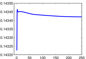
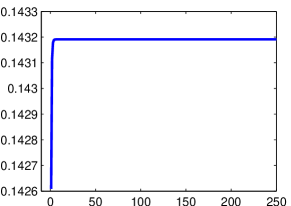
Before we present the experimental results, we describe the parameter settings used in the experiments. We randomly select 1000 data from the sub-dataset Pose27. There are different classes in this chosen subset. The image size is . We choose the size of core tensors to be . In the overall algorithm described in Fig. 2, we fix the number of iterations to as the recovered error does not vary much after iterations in most testing cases. For the RTR algorithm in line of Fig. 2, we use the default parameters proposed in the toolbox Manopt with the RTR maximal inner iteration number . For the first call to the RTR algorithm, we set the number of maximum outer iterations to with Manopt’s default initialization for ( in this case). For subsequent calls to RTR, we use iterations with the current as the initial values for memberships. In each overall iteration, we repeat the calls to Lines - in Fig. 2 twice to make sure that the factors stable.
| Evaluation metric | Mean | Std Var | Best | Worst |
|---|---|---|---|---|
| AC | 0.7120 | 0.0394 | 0.7630 | 0.6150 |
| NMI | 0.8189 | 0.0210 | 0.8467 | 0.7717 |
We conduct 20 runs for randomly initializing and . The statistics are reported in Table II. Under similar parameter settings, and for HOSVD Initialization I and and for HOSVD Initialization II, respectively. Both the random initialization and HOSVD initialization II strategies give comparable results and are are shown in Fig. 3(b). It should be noted that the reconstructed error does not improve with iterations. On the other hand, Fig. 3(a) shows the error curve for the HOSVD Initialization I strategy. As HOSVD gives the best estimate in terms of the model error, the error goes up initially when we move away from the best orthogonal factor to a membership factor. Finally, it stabilizes as shown in Fig. 3(a). This leads to the conclusion that among the three initialization strategies discussed in Section 4.3, HOSVD initialization I is the initialization of choice. In subsequent experiments, we initialize all the compared algorithms with HOSVD initialization I.
5.4 Algorithms and Comparisons
There exist many different clustering algorithms such as spectral clustering approaches [53] and the recent popular matrix factorization approaches[21, 54]. Since the Tucker decomposition is a multidimensional generalization of matrix factorization, we focus on the comparison between our proposed heterogeneous Tucker model with recent matrix factorization based clustering algorithms. The following methods are chosen as the benchmark for numerical comparisons. All the experiments are conducted on a desktop with an Intel Core i5-4670 CPU at 3.40GHz and with RAM of 8.00GB.
Multiplicative method for nonnegative matrix factorization (MM) [21]: This nonnegative matrix factorization algorithm is designed for vectorial data that are organized into a data matrix , i.e., each column represents an image. The matrix is factorized into the product of two nonnegative matrices such that . The columns of are regarded as the basis vectors and is interpreted as the weights, i.e., each data vector is obtained by a weighted linear combination of the the basis vectors. The matrix is also interpreted as containing clustering membership information.
Alternating least-squares algorithm (ALS) [54]: This algorithm is designed to solve the nonnegative matrix factorization problem of factorizing the nonnegative data matrix as by alternating optimization over the factor matrices and with the nonnegativity constraint.
Bayesian nonnegative matrix factorization (B-NFM) [55]: The model is based on the probabilistic framework in which the matrix factors and are regarded as random variables characterized by relevant statistical density functions. A Bayesian algorithm is proposed for solving the problem.
Projected gradient method for nonnegative matrix factorization (PGM) [22]: This algorithm results from simultaneously optimizing over the nonnegative factors and to approximately decompose a nonnegative data matrix as . Lin [22] proposes an efficient Newton algorithm.
Dual regularized co-clustering method (DRCC) [56]: The DRCC algorithm is a data clustering algorithm that is based on semi-nonnegative matrix tri-factorization with dual regularization over data graph and feature graph by exploiting the geometric structure of the data manifold and the feature manifold.
Nonnegative tri-factor tensor decomposition (Tri-ONTD) [27]: This algorithm is designed for 3-order tensorial data. It proposes a tensor decomposition with nonnegative factor matrices. Since it directly deals with tensor data, it can be considered as a benchmark algorithm for comparison with our proposed method.
Benchmark PCA-B: To demonstrate the benefits of the proposed model and, particularly, the Riemannian algorithm, we take the following revised algorithm as another benchmark algorithm. Instead of the problem (7), we propose to consider the problem (2) for a nonnegative membership matrix only, i.e., the constraint on the sum of each row to is lifted. This makes the problem formulation simpler, which can be solved by alternatively optimizing of each factor matrices, similar to the procedure in Fig. 2. In this case, optimizing becomes a quadratic programming problem with nonnegative constraints, which can be solved, e.g., using the Matlab function lsqlin.m.
PCA-Multinomial: The algorithm proposed in Fig. 2, which is based on the proposed heterogeneous Tucker decomposition model discussed in Section 2.2.
It should be noted that most above described algorithms perform better than (or comparable in some cases) to classical clustering algorithms, like the k-means [56, 27]. Hence, we do not compare with the classical clustering algorithms for vectorized data.
The implementations of the nonnegative matrix factorization algorithms MM, ALS, B-NFM, and PGM are in the Matlab NMF toolbox provided by Kasper Winther Joergensen. The Matlab code for DRCC is provided by the authors of [56]. We implement all the other algorithms. Our proposed algorithm, PCA-Multinomial, is implemented in Matlab using the Manopt toolbox [48].
Experiment I
We first test all the algorithms on the CBCL face dataset as this is the simplest case where there are only two clusters of images to be learned. The datasizes are chosen from to by for each class and the experiment results indicate that when size almost all the algorithms achieved similar accuracy. Under this size, we also test different tensor core sizes varying from to and find better results for our proposed tensor clustering method in the case of tensor core size .
Table III shows the means and variances (in brackets) for all the algorithms after runs. In Table III we see that all the algorithms are comparable for the case when the number of clusters is . For this experiment, DRCC has shown better performance than all the other algorithms. However, we also observe that in experiments when the performance of DRCC degrades. The benchmark algorithm PCA-B is slightly better than the proposed PCA-Multinomial by in AC. However, the variance of PCA-Multinomial is better in this experiment showing robustness of the Riemannian optimization algorithm.
| Evaluation metric | MM | ALS | B-NFM | PGM | DRCC | Tri-ONTD | PCA-B | PCA-Mulitnomial |
|---|---|---|---|---|---|---|---|---|
| AC | 0.6755 | 0.6424 | 0.6305 | 0.5976 | 0.7352 | 0.5764 | 0.6394 | 0.6208 |
| (5.494e-4) | (3.255e-4) | (3.594e-4) | (2.073e-3) | (1.367e-3) | (3.503e-5) | (3.301e-3) | (1.018e-4) | |
| NMI | 0.0928 | 0.0604 | 0.0509 | 0.0334 | 0.1766 | 0.0824 | 0.0669 | 0.0430 |
| (6.351e-4) | (2.505e-4) | (2.296e-4) | (7.794e-4) | (2.777e-3) | (1.836e-4) | (1.181e-3) | (5.524e-5) |
Experiment II
In this experiment, we assess the impact of the number of classes on the performance of all the algorithms. For this purpose, we conduct all the algorithms on the MNIST handwritten digits dataset. There are ten different classes, corresponding to the digits to . Most machine learning algorithms work well for the case of two clusters, i.e., . For , the performance of different algorithms varies, observing which is the main focus of the present experiment.
We randomly pick digits for training data according to the class number with images for each class. Once the classes are decided randomly, we run all the algorithms times each with randomly chosen digits in the classes. The experimental results are reported in Table IV in terms of AC and NMI evaluation metrics. It should be noted that Tri-ONTD algorithm fails for most of cases, and therefore, no results are reported. The results in Table IV show that the proposed PCA-Mulitnomial performs better in the cases of more than four classes. This is consistent with the results from the first experiment, where we observe a similar behavior. For , the performance of PCA-Multinomial is comparable with that of MM and PGM in both AC and NMI metrics.
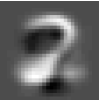
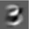
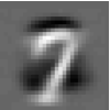
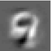
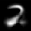
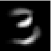
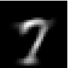
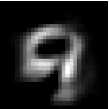
Figure 4 shows the reconstructed representatives from the learned centroids for , given by with the learned low dimensional centroids .
| Evaluation metric | MM | ALS | B-NFM | PGM | DRCC | PCA-B | PCA-Multinomial | |
|---|---|---|---|---|---|---|---|---|
| AC | 0.9173 | 0.9133 | 0.8820 | 0.9160 | 0.9013 | 0.8506 | 0.9114 | |
| (2.800e-4) | (2.6111e-4) | (1.644e-4) | (1.800e-4) | (3.589e-4) | (5.274e-3) | (1.700e-4) | ||
| NMI | 0.7351 | 0.7344 | 0.6806 | 0.7307 | 0.7115 | 0.6231 | 0.7252 | |
| (2.488e-3) | (1.654e-3) | (6.069e-4) | (1.792e-3) | (1.704e-3) | (1.492e-2) | (9.761e-4) | ||
| AC | 0.7140 | 0.6520 | 0.6780 | 0.7195 | 0.6575 | 0.6670 | 0.6800 | |
| (8.518e-4) | (8.611e-3) | (4.138e-4) | (5.325e-4) | (3.237e-3) | (4.576e-3) | (4.906e-4) | ||
| NMI | 0.4654 | 0.4181 | 0.4446 | 0.4680 | 0.4071 | 0.4184 | 0.4360 | |
| (1.726e-3) | (3.279e-3) | (5.964e-4) | (1.181e-3) | (3.278e-3) | (2.588e-3) | (7.243e-4) | ||
| AC | 0.6216 | 0.7112 | 0.6104 | 0.6764 | 0.6632 | 0.6960 | 0.7196 | |
| (7.731e-3) | (3.292e-4) | (3.839e-3) | (1.533e-3) | (2.792e-4) | (1.370e-3) | (1.334e-3) | ||
| NMI | 0.5201 | 0.5590 | 0.4992 | 0.5373 | 0.5198 | 0.5242 | 0.5547 | |
| (2.080e-3) | (1.018e-3) | (2.921e-3) | (9.196e-4) | (2.156e-4) | (1.130e-3) | (5.525e-4) | ||
| AC | 0.5370 | 0.5337 | 0.5156 | 0.5466 | 0.4983 | 0.5283 | 0.5540 | |
| (4.249e-3) | (3.626e-3) | (3.812e-3) | (4.257e-3) | (1.061e-3) | (5.234e-3) | (6.386e-3) | ||
| NMI | 0.4007 | 0.3852 | 0.3980 | 0.3962 | 0.3670 | 0.3850 | 0.4083 | |
| (9.891e-4) | (6.482e-4) | (1.197e-3) | (1.507e-3) | (1.348e-3) | (3.077e-3) | (1.945e-3) | ||
| AC | 0.5988 | 0.5974 | 0.5762 | 0.5940 | 0.6585 | 0.6074 | 0.6231 | |
| (8.816e-5) | (3.295e-3) | (1.051e-3) | (3.704e-3) | (1.789e-3) | (3.704e-3) | (5.618e-3) | ||
| NMI | 0.5382 | 0.5378 | 0.4972 | 0.5342 | 0.5629 | 0.5097 | 0.5401 | |
| (7.593e-4) | (1.607e-3) | (7.238e-4) | (9.776e-4) | (9.366e-4) | (1.204e-3) | (3.828e-4) | ||
| AC | 0.6455 | 0.6162 | 0.5930 | 0.5942 | 0.6270 | 0.5923 | 0.6485 | |
| (3.217e-3) | (8.523e-4) | (3.880e-3) | (3.267e-3) | (2.312e-3) | (4.726e-3) | (4.496e-3) | ||
| NMI | 0.5427 | 0.5496 | 0.4979 | 0.5152 | 0.5033 | 0.4944 | 0.5254 | |
| (5.694e-4) | (6.968e-4) | (1.329e-3) | (2.243e-3) | (3.711e-3) | (2.286e-3) | (2.367e-3) | ||
| AC | 0.5211 | 0.5567 | 0.5137 | 0.5302 | 0.5240 | 0.5224 | 0.5756 | |
| (1.251e-3) | (8.173e-4) | (5.528e-4) | (1.816e-3) | (7.867e-4) | (8.213e-4) | (3.569e-3) | ||
| NMI | 0.4621 | 0.4716 | 0.4343 | 0.4720 | 0.4493 | 0.4449 | 0.4774 | |
| (3.209e-4) | (3.473e-4) | (3.890e-4) | (5.279e-4) | (8.811e-4) | (1.130e-3) | (5.103e-4) | ||
| AC | 0.4980 | 0.4800 | 0.4474 | 0.4958 | 0.4668 | 0.4800 | 0.5126 | |
| (1.154e-3) | (9.220e-4) | (5.823e-4) | (1.833e-3) | (2.846e-3) | (2.761e-3) | (1.785e-3) | ||
| NMI | 0.4470 | 0.4505 | 0.4089 | 0.4516 | 0.4053 | 0.4142 | 0.4461 | |
| (7.543e-4) | (5.267e-4) | (3.474e-4) | (2.051e-3) | (3.402e-3) | (8.642e-4) | (1.146e-3) |
Experiment III
A test similar to Experiment II is conducted on the PIE dataset to further confirm the main conclusion form Experiment II, that the performance of PCA-Multinomial is better when are a larger number of clusters are sought. We do not report the performance of the Tri-ONTD algorithm as it does not provide meaningful results in our experiments. The PIE dataset contains clusters, each with objects. In this experiment, we test the algorithms on the data of , , , , , , and clusters, respectively. To maintain the data size to be around , we randomly pick images for the case of cluster , for , for , for , for , for , and for . The procedure is repeated for runs. In the last case, the data size is and each run is with different clusters.
The results are collected in Table V. PCA-Multinomial performs better than the others, except for the case , where MM takes the lead. Part of this behavior is due to lack of sufficient data in the case of cluster . However NMI scores are all over , except for the case . Both DRCC and PCA-B do not show meaningful results on this dataset.
| Evaluation metric | MM | ALS | B-NFM | PGM | DRCC | PCA-B | PCA-Multinomial | |
|---|---|---|---|---|---|---|---|---|
| AC | 0.6088 | 0.5633 | 0.6192 | 0.5120 | 0.2745 | 0.4314 | 0.6533 | |
| (4.563e-4) | (2.101e-4) | (4.311e-4) | (7.590e-4) | (2.736e-4) | (1.018e-3) | (8.749e-4) | ||
| NMI | 0.8066 | 0.7791 | 0.8099 | 0.7540 | 0.5652 | 0.6828 | 0.8634 | |
| (2.222e-4) | (4.083e-5) | (9.111e-5) | (9.963e-5) | (3.231e-4) | (3.197e-4) | (2.484e-4) | ||
| AC | 0.6182 | 0.5730 | 0.5968 | 0.5482 | 0.2504 | 0.4125 | 0.6781 | |
| (5.719e-4) | (3.549e-3) | (1.884e-4) | (1.362e-3) | (2.215e-4) | (1.318e-3) | (9.944e-4) | ||
| NMI | 0.8027 | 0.7790 | 0.7955 | 0.7580 | 0.5140 | 0.6555 | 0.8742 | |
| (2.504e-4) | (6.398e-4) | (2.789e-5) | (2.096e-4) | (2.995e-4) | (8.198e-4) | (1.483e-4) | ||
| AC | 0.6112 | 0.5964 | 0.6147 | 0.5951 | 0.2875 | 0.4228 | 0.6990 | |
| (1.625e-4) | (6.027e-4) | (1.777e-3) | (5.105e-4) | (4.925e-4) | (6.271e-4) | (7.863e-4) | ||
| NMI | 0.7899 | 0.7812 | 0.7896 | 0.7775 | 0.5266 | 0.6491 | 0.8480 | |
| (1.084e-4) | (4.319e-4) | (1.928e-4) | (1.633e-4) | (2.659e-4) | (1.115e-4) | (8.585e-5) | ||
| AC | 0.5799 | 0.6197 | 0.6138 | 0.5930 | 0.2621 | 0.3911 | 0.7118 | |
| (2.292e-3) | (9.405e-4) | (9.892e-4) | (3.646e-4) | (3.578e-4) | (1.227e-3) | (1.384e-3) | ||
| NMI | 0.7552 | 0.7769 | 0.7717 | 0.7553 | 0.4461 | 0.5949 | 0.8516 | |
| (3.956e-4) | (6.884e-4) | (5.941e-4) | (1.132e-4) | (1.461e-4) | (5.438e-4) | (1.716e-4) | ||
| AC | 0.6224 | 0.6214 | 0.6329 | 0.6408 | 0.2619 | 0.4212 | 0.6877 | |
| (2.564e-3) | (1.448e-3) | (4.329e-4) | (8.523e-4) | (2.704e-4) | (4.090e-3) | (4.106e-3) | ||
| NMI | 0.7470 | 0.7610 | 0.7586 | 0.7519 | 0.4033 | 0.5669 | 0.8153 | |
| (4.750e-4) | (5.707e-4) | (1.975e-4) | (3.880e-4) | (3.592e-4) | (2.179e-3) | (5.873e-4) | ||
| AC | 0.6367 | 0.6387 | 0.5892 | 0.6511 | 0.2962 | 0.4865 | 0.7329 | |
| (6.368e-4) | (1.002e-2) | (5.057e-3) | (2.232e-3) | (2.326e-3) | (6.932e-3) | (1.352e-3) | ||
| NMI | 0.7290 | 0.7433 | 0.7089 | 0.7377 | 0.3836 | 0.5917 | 0.8010 | |
| (5.039e-4) | (2.437e-3) | (8.551e-4) | (4.477e-4) | (1.570e-3) | (3.972e-3) | (7.787e-4) | ||
| AC | 0.6690 | 0.6256 | 0.6321 | 0.6285 | 0.3809 | 0.4785 | 0.6523 | |
| (1.073e-3) | (2.698e-3) | (9.592e-4) | (1.396e-3) | (9.553e-3) | (3.036e-2) | (1.634e-2) | ||
| NMI | 0.6512 | 0.6797 | 0.6382 | 0.6289 | 0.3110 | 0.4403 | 0.6803 | |
| (4.287e-3) | (5.646e-4) | (6.623e-4) | (1.509e-3) | (1.269e-2) | (3.941e-2) | (1.057e-2) |
Experiment IV
In this experiment, we test the algorithms on both the ORL dataset of subjects with images and the YaleB extended dataset of subjects with images.
For the ORL dataset, we randomly choose subjects for five runs of the algorithm. The results in Table VI show that the PCA-Multinomial algorithm outperforms all the other algorithms on the ORL dataset in terms of both AC and NMI scores.
For the YaleB extended dataset, we use all the images. Hence, only one test is conducted and the results are summarized in Table VI. It should be noted that all the algorithms show poor performance on the YaleB dataset although the PCA-Multinomial algorithm has relatively better performance. This is due to the large variants among this dataset.
| Evaluation metric | MM | ALS | B-NFM | PGM | DRCC | PCA-B | PCA-Multinomial | |
| ORL | AC | 0.6440 | 0.6820 | 0.6280 | 0.6300 | 0.5580 | 0.6360 | 0.7340 |
| (3.730e-3) | (9.070e-3) | (8.070e-3) | (3.650e-3) | (4.870e-3) | (5.130e-3) | (2.230e-3) | ||
| NMI | 0.7308 | 0.7269 | 0.7107 | 0.7236 | 0.6498 | 0.6968 | 0.7996 | |
| (1.842e-3) | (5.946e-3) | (2.688e-3) | (1.668e-3) | (8.727e-4) | (5.467e-3) | (7.283e-4) | ||
| YaleB | AC | 0.2175 | 0.2270 | 0.2104 | 0.2084 | 0.1002 | 0.2117 | 0.3293 |
| NMI | 0.3534 | 0.3470 | 0.3508 | 0.3477 | 0.1455 | 0.3402 | 0.4772 |
Experiment V
In this experiment, we test the PCA-Multinomial algorithm against the benchmark PCA-B algorithm on the DynTex++ dataset. The other algorithms are not appropriate for this dataset. Tri-ONTD works for matrix data, i.e., it can handle a set of images or -order tensors, whereas the rest work with vectorial data, i.e., can handle only matrices. The core tensor size is fixed to . We conduct tests on the cases of up to classes. In each test, the total number of training video subsequences is determined to for classes, for classes, for classes, for classes, for classes and classes, and for classes. The classes are randomly chosen. For each case, five runs are conducted by randomly choosing video subsequences in the chosen classes, except for the case of two classes, where the only subsequences are all used in a single run.
The results are summarized in Table VII. Particularly, the results show the challenging nature of clustering dynamic textures for classes. In all the cases, PCA-Multinomial algorithm consistently performs better than the benchmark PCA-B. This once again confirms the benefits of using the RTR algorithm based on the Riemannian geometry of the multinomial manifold.
| Models | Evaluation metric | 2 Classes | 3 Classes | 4 Classes | 6 Classes | 8 Classes | 10 Classes | 12 Classes |
| PCA-B | AC | 0.5550 | 0.4230 | 0.3727 | 0.2983 | 0.2507 | 0.1937 | 0.2024 |
| - | ( 4.069e-3) | ( 1.429e-3) | ( 4.088e-4) | ( 5.244e-4) | ( 8.527e-5) | (3.416e-4) | ||
| NMI | 0.1034 | 0.1849 | 0.2261 | 0.2079 | 0.2259 | 0.2451 | 0.2520 | |
| - | ( 8.471e-3) | ( 1.667e-3) | ( 4.817e-4) | ( 2.926e-4) | ( 1.057e-3) | (9.549e-5) | ||
| PCA-Multinomial | AC | 0.7901 | 0.5827 | 0.5767 | 0.3842 | 0.4007 | 0.3300 | 0.2980 |
| - | ( 5.522e-4) | ( 6.350e-3) | ( 1.361e-3) | ( 1.325e-3) | ( 1.272e-3) | ( 2.519e-4) | ||
| NMI | 0.4056 | 0.2047 | 0.3360 | 0.3012 | 0.3538 | 0.3285 | 0.3444 | |
| - | ( 5.924e-4) | ( 6.116e-4) | ( 9.165e-4) | ( 5.356e-4) | ( 4.801e-4) | ( 1.563e-4) |
6 Conclusion
We proposed a heterogeneous Tucker decomposition model for tensor clustering. The model simultaneously conducts dimensionality reduction and optimizes membership representation. The dimensionality reduction is conducted along the first -modes while optimizing membership on the last mode of tensorial data. The resulting optimization problem is a nonlinear optimization problem over the special matrix multinomial manifold. To apply the Riemannian trust region algorithm to the problem, we explored the Riemannian geometry of the manifold under the Fisher information metric. Finally, we implemented the clustering algorithms based on the Riemannian optimization. We used a number of real-world datasets to test the proposed algorithms and compared them with existing state-of-the-art nonnegative matrix factorization methods. Numerical results illustrate the good clustering performance of the proposed algorithms particularly in the case of higher class numbers.
Further work can be carried out in several different directions. For example, in the current work we use an alternating procedure to optimize over all the factor matrices , , , . However, this is not the only way to solve the problem. As the constraint for defines the Stiefel manifold, the overall optimization problem (4) is defined over the product manifold of Stiefel manifolds and one pn the multinomial manifold. This can be directly optimized over the entire product of manifolds, e.g., using Manopt. Another issue that needs to be further investigated is how to scale the algorithm for (6) to high-dimensional data.
Acknowledgments
This research was supported under Australian Research Council’s Discovery Projects funding scheme (project number DP130100364). This work is also partially supported by the National Natural Science Foundation of China (No. 61370119, 61133003 and 61390510) and the Natural Science Foundation of Beijing (No. 4132013). Bamdev Mishra is supported as an FRS-FNRS research fellow (Belgian Fund for Scientific Research).
References
- [1] B. Schölkopf and A. Smola, Learning with Kernels. Cambridge, Massachusetts: The MIT Press, 2002.
- [2] H. Lua, K. N. Plataniotisb, and A. N. Venetsanopoulos, “A survey of multilinear subspace learning for tensor data,” Pattern Recognition, vol. 44, pp. 1540–1551, 2011.
- [3] X. Guo, L. Zhang, and X. Huang, “Hyperspectral image noise reduction based on rank-1 tensor decomposition,” ISPRS Journal of Photogrammetry and Remote Sensing, vol. 83, pp. 50–63, 2013.
- [4] J. Sun, H. Zeng, H. Liu, Y. Lu, and Z. Chen, “CubeSVD: A novel approach to personalized web search,” in Proceedings of the 14th international conference on World Wide Web, 2005.
- [5] D. Cai, X. He, and J. Han, “Tensor space model for document analysis,” in Proceedings of the 29th annual international ACM SIGIR conference on Research and development in information retrieval, 2006, pp. 625 – 626.
- [6] R. Forsati, M. Mahdavi, M. Shamsfard, and M. R. Meybodi, “Efficient stochastic algorithms for document clustering,” Information Sciences, vol. 220, pp. 269–291, 2013.
- [7] T. G. Kolda, “Multilinear operators for higher-order decompositions,” Sandia National Laboratories, Tech. Rep., 2006.
- [8] T. G. Kolda and B. W. Bader, “Tensor decompositions and applications,” SIAM Review, vol. 51, no. 3, pp. 455–500, 2009.
- [9] G. A. Shaw and H. hua K. Burke, “Spectral imaging for remote sensing,” Lincoln Laboratory Journal, vol. 14, no. 1, pp. 3–28, 2003.
- [10] A. K. Jain, M. N. Murty, and P. J. Flynn, “Data clustering: A Review,” ACM Computing Surveys, vol. 31, no. 3, pp. 264–323, 1999.
- [11] C. Bishop, Pattern Recognition and Machine Learning, ser. Information Science and Statistics. Springer, 2006.
- [12] G. Golub and C. van Loan, Matrix Computations, 3rd ed. Maryland: The Johns Hopkins University Press, 1996.
- [13] S. Aja-Fernández, G. R. Luis, D. Tao, and X. Li, Tensors in Image Processing and Computer Vision. Springer, 2009.
- [14] Y. Tang, R. Salakhutdinov, and G. Hinton, “Tensor analyzers,” in Proceedings of the 30th International Conference on Machine Learning, Atlanta, USA, 2013.
- [15] A. Shashua and T. Hazan, “Non-negative tensor factorization with applications to statistics and computer vision,” in Proceedings of International Conference on Machine Learning (ICML), 2005, pp. 792–799.
- [16] M. Morup, “Applications of tensor (multiway array) factorizations and decompositions in data mining,” Wiley Interdisciplinary Reviews: Data Mining and Knowledge Discovery, vol. 1, no. 1, pp. 24–40, 2011.
- [17] H. Kiers, “Towards a standardized notation and terminology in multiway analysis,” Journal of Chemometrics, vol. 14, no. 3, pp. 105–122, 2000.
- [18] L. DeLathauwer, B. DeMoor, and J. Vandewalle, “A multilinear singular value decomposition,” SIAM Journal of Matrix Analysis and Applications, vol. 21, no. 4, pp. 1253–1278, 2001.
- [19] ——, “On the best rank-1 and rank-() approximation of higherorder tensors,” SIAM Journal of Matrix Analysis and Applications, vol. 21, p. 1324–1342, 2000.
- [20] D. D. Lee and H. S. Seung, “Learning the parts of objects by non-negative matrix factorization,” Nature, vol. 401, no. 6755, p. 788–791, 1999.
- [21] ——, “Algorithms for non-negative matrix factorization,” in Advances in Neural Information Processing Systems (NIPS), T. K. Leen, T. G. Diettercih, and V. Tresp, Eds., vol. 13. MIT Press, 2001, pp. 556–562.
- [22] C. Lin, “Projected gradient methods for nonnegative matrix factorization,” Neural Computation, vol. 19, no. 10, p. 2756–2779, 2007.
- [23] M. Welling and M. Weber, “Positive tensor factorization,” Pattern Recognition Letters, vol. 22, pp. 1255–1261, 2001.
- [24] M. P. Friedlander and K. Hatz, “Computing non-negative tensor factorizations,” Optimization Methods and Software, vol. 23, no. 4, pp. 631–647, 2008.
- [25] J. Liu, J. Liu, P. Wonka, and J. Ye, “Sparse non-negative tensor factorization using columnwise coordinate descent,” Pattern Recognition, vol. 45, pp. 649–656, 2012.
- [26] F. Wu, X. Tan, Y. Yang, D. Tao, S. Tang, and Y. Zhuang, “Supervised nonnegative tensor factorization with maximum-margin constraint,” in Proceedings of the Twenty-Seventh AAAI Conference on Artificial Intelligence, 2013, pp. 962–968.
- [27] Z. Y. Zhang, T. Li, and C. Ding, “Non-negative tri-factor tensor decomposition with applications,” Knowledge Information Systems, vol. 34, pp. 243–265, 2013.
- [28] H. Liu, Z. Wu, X. Li, D. Cai, and T. S. Huang, “Constrained nonnegative matrix factorization for image representation,” IEEE Transactions on Pattern Analysis and Machine Intelligence, vol. 34, no. 7, pp. 1299–1311, 2012.
- [29] M. Vichi, R. Rocci, and H. Kiers, “Simultaneous component and clustering models for three-way data: Within and between approaches,” Journal of Classification, vol. 24, no. 1, pp. 71–98, 2007.
- [30] E. Acar and B. Yener, “Unsupervised multiway data analysis: A literature survey,” IEEE Transactions on Knowledge and Data Engineering, vol. 21, no. 1, pp. 6–20, 2009.
- [31] W. Peng and T. Li, “Tensor clustering via adaptive subspace iteration,” Intelligent Data Analysis, vol. 15, pp. 695–713, 2011.
- [32] Y. Sun, J. Gao, X. Hong, Y. Guo, and C. J. Harris, “Dimensionality reduction assisted tensor clustering,” in Proceedings of International Joint Conference on Neural Networks (JCNN), 2014.
- [33] P.-A. Absil, R. Mahony, and R. Sepulchre, Optimization algorithms on matrix manifolds. Princeton University Press, 2008.
- [34] B. Mishra, G. Meyer, F. Bach, and R. Sepulchre, “Low-rank optimization with trace norm penalty,” SIAM Journal on Optimization, vol. 23, no. 4, pp. 2124–2149, 2013.
- [35] B. Vandereycken, “Riemannian and multilevel optimization for rank constrained matrix problems,” PhD Thesis, Faculty of Engineering, Katholieke Universiteit Leuven, Address, B-3001 Leuven, Belgium, 2010.
- [36] G. Meyer, “Geometric optimization algorithms for linear regression on fixed-rank matrices,” PhD Thesis, University of Lige, Address, B-4031 Liège, Belgium, 2011.
- [37] N. Boumal, “Optimization and estimation on manifolds,” PhD Thesis, Université catholique de Louvain, Address, B-1348 Louvain-la-Neuve, Belgium, 2014.
- [38] Y. Xie, J. Ho, and B. Vemuri, “On a nonlinear generalization of sparse coding and dictionary learning,” Journal of Machine Learning Research: Workshop and Conference Proceedings, vol. 28, no. 3, pp. 1480–1488, 2013.
- [39] M. Harandi, R. Hartley, C. Shen, B. Lovell, and C. Sanderson, “Extrinsic methods for coding and dictionary learning on Grassmann manifolds,” arXiv:1401.8126, pp. 1–41, 2014.
- [40] Y. M. Lui, “Advances in matrix manifolds for computer vision,” Image and Vision Computing, vol. 30, pp. 380–388, 2012.
- [41] A. Kapteyn, H. Neudecker, and T. Wansbeek, “An approach to -mode components analysis,” Psychometrika, vol. 51, pp. 269–275, 1986.
- [42] P. Tseng and S. Yun, “A coordinate gradient descent method for linearly constrained smooth optimization and support vector machines training,” Computational Optimization and Applications, p. to appear, 2015.
- [43] J. M. Lee, Introduction to Smooth Manifolds, ser. Graduate Texts in Mathematics. Springer, 2002, vol. 218.
- [44] G. Lebanon and J. Lafferty, “Hyperplane margin classifiers on the multinomial manifold,” in Proceedings of the 21st International Conference on Machine Learning, Banff, Canada, 2004.
- [45] D. Zhang, X. Chen, and W. S. Lee, “Text classification with kernels on the multinomial manifold,” in Proceedings of the 28th annual international ACM SIGIR Conference on Research and Development in Information Retrieval, 2005, pp. 266–273.
- [46] R. Inokuchi and S. Miyamoto, “-means clustering on the multinomial manifold,” Lecture Notes in Computer Science, vol. 4617, pp. 261–268, 2007.
- [47] K. B. Petersen and M. S. Pedersen, “The matrix cookbook,” Oct 2008, versio 20081110. [Online]. Available: http://www2.imm.dtu.dk/pubdb/p.php?3274
- [48] N. Boumal, B. Mishra, P.-A. Absil, and R. Sepulchre, “Manopt, a Matlab toolbox for optimization on manifolds,” Journal of Machine Learning Research, vol. 15, pp. 1455–1459, 2014. [Online]. Available: http://www.manopt.org
- [49] D. G. Luenberger, and Y. Ye, Linear and nonlinear programming. Springer, 2008.
- [50] D. Cai, X. He, X. Wang, H. Bao, and J. Han, “Locality preserving nonnegative matrix factorization,” in Proc. of Int. Joint Conference on Artificial Intelligence (IJCAI), 2009.
- [51] S. S. Chen, D. L. Donoho, and M. A. Saunders, “Atomic decomposition by basis pursuit,” SIAM Review, vol. 43, no. 1, pp. 129–159, Jan. 2001.
- [52] D. Cai, X. He, J. Han, and T. S. Huang, “Graph regularized non-negative matrix factorization for data representation. , 33(8):, 2011.” IEEE Transactions on Pattern Analysis and Machine Intelligence, vol. 33, no. 8, pp. 1548–1560, 2011.
- [53] J. Shi and J. Malik, “Normalized cuts and image segmentation,” IEEE Transactions on Pattern Analysis and Machine Intelligence, vol. 22, pp. 888–905, 2000.
- [54] H. Kim and H. Park, “Sparse non-negative matrix factorization via alternating non-negativity-constrained least squares for microarray data analysis,” Bioinformatics, vol. 23, no. 12, pp. 1495–1502, 2007.
- [55] M. Schmidt, O. Winther, and L. Hansen, “Bayesian non-negative matrix factorization,” in Lecture Notes in Computer Science (LNCS): Proc. of International Conf on Independent Component Analysis and Signal Separation, vol. 5541, 2009, pp. 540–547.
- [56] Q. Gu and J. Zhou, “Co-clustering on manifolds,” in The 15th ACM SIGKDD International Conference on Knowledge Discovery and Data Mining (KDD), Paris, France, 2009.