Evolution of mass functions of coeval stars through wind mass loss and binary interactions

Abstract

Accurate determinations of stellar mass functions and ages of stellar populations are crucial to much of astrophysics. We analyse the evolution of stellar mass functions of coeval main sequence stars including all relevant aspects of single- and binary-star evolution. We show that the slope of the upper part of the mass function in a stellar cluster can be quite different to the slope of the initial mass function. Wind mass loss from massive stars leads to an accumulation of stars which is visible as a peak at the high mass end of mass functions, thereby flattening the mass function slope. Mass accretion and mergers in close binary systems create a tail of rejuvenated binary products. These blue straggler stars extend the single star mass function by up to a factor of two in mass and can appear up to ten times younger than their parent stellar cluster. Cluster ages derived from their most massive stars that are close to the turn-off may thus be significantly biased. To overcome such difficulties, we propose the use of the binary tail of stellar mass functions as an unambiguous clock to derive the cluster age because the location of the onset of the binary tail identifies the cluster turn-off mass. It is indicated by a pronounced jump in the mass function of old stellar populations and by the wind mass loss peak in young stellar populations. We further characterise the binary induced blue straggler population in star clusters in terms of their frequency, binary fraction and apparent age.

1. Introduction

Stellar mass functions are important for population studies, both nearby and at high redshift. Mass functions are not static but change their shape when the frequencies of stars or their masses are altered over time (Scalo 1986; Kroupa et al. 2013). Possible causes include the evaporation of stars and mass segregation in star clusters (de Grijs et al. 2002; McLaughlin & Fall 2008; Harfst et al. 2010; Habibi et al. 2013) and mass loss in the course of stellar evolution (Langer 2012). These mechanisms leave characteristic fingerprints in mass functions from which insights into the evolutionary status of stellar populations and the mechanisms themselves can be gained.

Massive stars are subject to strong stellar wind mass loss, which decreases their masses already on the main sequence (MS), directly affecting mass functions. Furthermore, it emerges that binary stars play an important role in stellar populations of various ages and even dominate the evolution of massive stars (Sana et al. 2012). The multiplicity fraction, i.e. the number of multiple stars divided by the total number of stellar systems, is larger for higher masses (e.g. Bastian et al. 2010; Duchêne & Kraus 2013): it exceeds 40% for solar like stars (F, G and K stars) and 70% for the most massive stars (O-stars). In close binaries, mass is exchanged between the binary components during Roche lobe overflow (RLOF) or in stellar mergers, directly affecting stellar masses and hence the mass function. The mass gainers are rejuvenated and can appear much younger than they really are. Some mass gainers may also be visible as blue straggler stars (Braun & Langer 1995; Dray & Tout 2007; Geller & Mathieu 2011).

The determination of stellar ages is a fundamental task in stellar astrophysics (Soderblom 2010) that can be biased by rejuvenated binary products. Various methods are used to determine stellar ages. The surface properties of individual stars can be compared with evolutionary model predictions, e.g., luminosity, surface temperature or surface gravity (Holmberg et al. 2007; Schneider et al. 2014a), rotation rates in low mass stars (Barnes 2007) or surface nitrogen abundances in massive stars (Köhler et al. 2012). In star clusters, the most widely used age determination method compares the main sequence turn-off with theoretical isochrones (e.g. Naylor & Jeffries 2006; Monteiro et al. 2010). Close binary evolution such as mass transfer and stellar mergers leads to spurious or inaccurate results in all of these methods. To derive unambiguous age estimates one must be able to distinguish between rejuvenated binary products and genuinely single stars.

In this paper we investigate how the modulation of stellar mass functions by single and binary star evolution can be used both to identify binary products and to derive unambiguous stellar ages. More generally, we explore what can be learned about stellar evolution and the evolutionary status of whole stellar populations from observed mass functions. We also investigate quantitatively how single and binary star evolution influence the determination of initial mass functions. To that end, we perform detailed population synthesis calculations of coeval stellar populations using a rapid binary evolution code.

We describe our method in Sec. 2 and present mass functions of coeval single and binary star populations of ages ranging from $3\,\mathrm{Myr}$ to $1\,\mathrm{Gyr}$ in Sec. 3. Through binary interactions, blue straggler stars are formed in our models. We characterise their binary fraction and ages, and compare their predicted frequencies to those found in Galactic open star clusters in Sec. 4. Blue straggler stars predominantly populate the high mass end of mass functions and may bias determinations of stellar cluster ages. We show how to use mass functions to overcome such biases when determining cluster ages in Sec. 5 and conclude in Sec. 6.

2. Method

We compute the evolution of single and close, interacting binary stars and construct, at predefined ages, mass functions by counting how many stars of certain masses exist. This approach ensures that we factor in all the relevant single and binary star physics to investigate their influence on the present-day mass function (PDMF).

The initial parameter space of binaries is large compared to that of single stars, which essentially consists of the initial mass. In binaries, there are two masses, the orbital separation, the eccentricity of the orbit and the relative orientation of the spin axis of both stars. We apply some standard simplifications to reduce this huge parameter space: we impose circular orbits and that both stellar spins are aligned with the orbital angular momentum. All our models are calculated for a metallicity $Z=0.02$ (unless stated otherwise). Furthermore we focus on the main sequence because stars spend typically $90\%$ of their life in this evolutionary stage. Still, we need to follow the evolution of a large number of stellar systems to sample the remaining binary parameter space and to resolve effects at the high mass end of the PDMF. Hence, we work with a rapid binary evolution code.

2.1. Rapid binary evolution code

We use the binary population and nucleosynthesis code of Izzard et al. (2004, 2006, 2009) with modifications due to de Mink et al. (2013) which is based on the rapid binary evolution code of Hurley et al. (2002). This code uses analytic formulae (Hurley et al. 2000) fitted to detailed single star evolutionary models (Pols et al. 1998) to approximate the evolution of single stars for a wide range of masses and metallicities.

The fitting formulae of Hurley et al. (2000) are based on detailed stellar model sequences of stars with mass up to $50\,{\rm M}_{\odot}$ (Pols et al. 1998). The evolution of stars with mass in excess of $50\,{\rm M}_{\odot}$ is thus based on extrapolations of the original fitting formulae. The MS lifetime, $\tau_{\mathrm{MS}}$, is particularly inaccurately extrapolated by the appropriate fit, so we replace it with a logarithmic tabular interpolation of the MS lifetimes taken directly from the models of Pols et al. (1998) in the mass range $20\leq M\leq 50\,{\rm M}_{\odot}$. More massive than this we extrapolate the final two masses in the grid of detailed models (Pols et al. 1998). This results in a reduction of the MS lifetime of e.g. a $100\,{\rm M}_{\odot}$ star at $Z=0.02$ from $3.5$ to $2.9\,\mathrm{Myr}$, i.e. in a reduction of $17\%$, which is in agreement with state-of-the-art non-rotating detailed stellar models of Brott et al. (2011) and Ekström et al. (2012).

Stellar wind mass loss for stars with luminosities $L>4000\,{\rm L}_{\odot}$ is given by Nieuwenhuijzen & de Jager (1990). This recipe is modified by a factor $Z^{0.5}$ according to Kudritzki et al. (1989) to mimic the impact of the metallicity $Z$ on wind mass loss rates.

Binary stars can exchange mass either by RLOF, wind mass transfer or merging. RLOF occurs when one star (hereafter the donor) fills its Roche lobe and transfers mass to its companion (hereafter the accretor) through the inner Lagrangian point. Depending on the physical state of the donor star one distinguishes between Case A, B and C mass transfer. Following the definition of Kippenhahn & Weigert (1967), Case A mass transfer occurs during core hydrogen burning, Case B after the end of core hydrogen burning and Case C, defined by Lauterborn (1970), after the end of core helium burning.

Our binary evolution code differs from Hurley et al. (2002) in its treatment of RLOF. For stable mass transfer it is expected that the stellar radius $R$ adjusts itself to the Roche lobe radius $R_{\mathrm{L}}$, i.e. $R\approx R_{\mathrm{L}}$. Whenever RLOF occurs ($R>R_{\mathrm{L}}$) we remove as much mass as needed to shrink the donor star back into its Roche lobe. The resulting mass transfer and mass accretion rates are capped by the thermal timescales of the donor and accretor, respectively.

We follow Hurley et al. (2002) to determine the occurrence of common envelope evolution and contact phases that lead to stellar mergers. MS mergers are expected either if the initial orbital separation is so small that both stars fill their Roche lobes and thus come into physical contact or if the mass ratio of the accretor to the donor star falls below a certain limit at the onset of mass transfer, $q=M_{2}/M_{1}<q_{\mathrm{crit}}$, which drives the accretor out of thermal equilibrium and hence results in a contact system (e.g. Ulrich & Burger 1976; Kippenhahn & Meyer-Hofmeister 1977; Neo et al. 1977; Wellstein et al. 2001). The critical mass ratio is approximately $q_{\mathrm{crit,MS}}=0.56$ for MS stars (de Mink et al. 2007), $q_{\mathrm{crit,HG}}=0.25$ if the donor star is a Hertzsprung gap star and is given by a fitting formula if the donor star has a deep convective envelope (Hurley et al. 2002).

Mass transfer because of either stable RLOF or during a stellar merger makes the mass gainers appear younger than they really are (Braun & Langer 1995; van Bever & Vanbeveren 1998; Dray & Tout 2007). Such rejuvenated stars may stand out as blue stragglers in Hertzsprung–Russell (HR) diagrams. Rejuvenation is handled following Tout et al. (1997) and Hurley et al. (2002) but with improvements as described in Glebbeek & Pols (2008) and de Mink et al. (2013). The apparent age $T$ of a star is given by the amount of burnt fuel compared to the total available. For a star with MS lifetime $\tau_{\mathrm{MS}}$ we therefore have (in a linear approximation) $T=f_{\mathrm{burnt}}\tau_{\mathrm{MS}}$ where $f_{\mathrm{burnt}}=M_{\mathrm{burnt}}/M_{\mathrm{available}}$ is the mass ratio of the burnt to totally available fuel. After mass transfer onto a MS star with a convective core, the mass of the already burnt fuel is given by the fraction of burnt material, $f_{\mathrm{burnt}}$, times the convective core mass before mass transfer, $M_{\mathrm{c}}$ (primes indicate quantities after mass transfer). After mass transfer, the convective core and hence the available fuel of the accretor grow in mass, i.e. $M^{\prime}_{\mathrm{c}}>M_{\mathrm{c}}$, because the total stellar mass increases (and vice versa for the donor star). Thus, the fraction of burnt fuel after mass transfer is $f^{\prime}_{\mathrm{burnt}}=f_{\mathrm{burnt}}M_{\mathrm{c}}/M^{\prime}_{\mathrm{c}}$ and the apparent age, $T^{\prime}=f^{\prime}_{\mathrm{burnt}}\tau_{\mathrm{MS}}^{\prime}$, is

$$T^{\prime}=\frac{M_{\mathrm{\mathrm{c}}}}{M_{\mathrm{c}}^{\prime}}\frac{\tau_{\mathrm{MS}}^{\prime}}{\tau_{\mathrm{MS}}}T.$$ (1)

This equation holds for the accretor and also for the donor when setting $M_{\mathrm{c}}=M_{\mathrm{c}}^{\prime}$ (no burnt fuel is mixed out of the core upon mass loss from the stellar surface) and shows that the accreting stars rejuvenate upon mass transfer ($T^{\prime}<T$ because $M^{\prime}_{\mathrm{c}}\geq M_{\mathrm{c}}$ and $\tau_{\mathrm{MS}}^{\prime}<\tau_{\mathrm{MS}}$) while the donor stars age ($T^{\prime}>T$ because $\tau_{\mathrm{MS}}^{\prime}>\tau_{\mathrm{MS}}$). The accretor and donor will have burnt less (more) fuel than a single star of the same mass that did not accrete (lose) mass. If stars do not have convective cores, e.g., stars with initial masses in the range $0.3\leq M/{\rm M}_{\odot}\leq 1.3$ or Hertzsprung gap stars which have radiative cores, we set $M_{\mathrm{c}}=M_{\mathrm{c}}^{\prime}$ because no fresh fuel is expected to be mixed into their cores.

To model the rejuvenation of MS mergers we follow de Mink et al. (2013): first, we assume that a fraction $f_{\mathrm{loss}}$ of the total mass $M_{3}=M_{1}+M_{2}$ is lost during the merger; we adopt $f_{\mathrm{loss}}=0.1$. Second, we approximate the core mass fraction $f_{\mathrm{c}}$ of MS stars according to fitting functions (Glebbeek & Pols 2008) and estimate the apparent age $T_{3}$ of the newly formed merged star from,

$$T_{3}=\tau_{\mathrm{MS,3}}\cdot\frac{f_{\mathrm{c,1}}\cdot\frac{T_{1}}{\tau_{\mathrm{MS,1}}}+f_{\mathrm{c,2}}\cdot\frac{T_{2}}{\tau_{\mathrm{MS,2}}}}{f_{\mathrm{c,3}}^{\mathrm{eff}}},$$ (2)

where $T_{1}$ and $T_{2}$ are the effective ages, $f_{\mathrm{c,1}}$ and $f_{\mathrm{c,2}}$ are the core mass fractions of the progenitor stars and $\tau_{\mathrm{MS}}$ denotes the MS lifetime of the corresponding star. The denominator contains the effective core mass fraction $f_{\mathrm{c,3}}^{\mathrm{eff}}=f_{\mathrm{c,3}}+f_{\mathrm{mix}}\cdot(1-f_{\mathrm{c,3}})$ of the merger product which is given by its core mass fraction modified by an additional mixing of $f_{\mathrm{mix}}=10\%$ of the hydrogen-rich envelope. The resulting rejuvenation is less than in the original Hurley et al. (2002) code, where it is assumed that the whole star is mixed, and closer to that seen in hydrodynamic and smoothed particle hydrodynamics simulations of stellar mergers (e.g. Lombardi et al. 1995; Sills et al. 1997, 2001; Glebbeek & Pols 2008; Glebbeek et al. 2013).

2.2. Initial distribution functions

We set up a grid of stellar systems to cover the parameter space of single and binary stars and assign each stellar system $j$ a probability of existence $\delta p_{j}$. The probabilities $\delta p_{j}$ are calculated from $\delta p_{j}=\Psi\delta\ln V$ where $\Psi$ is a distribution function of the initial masses and the initial orbital periods and $\delta\ln V$ is the volume of the parameter space filled by the stellar system $j$. The initial distribution function, $\Psi$, reads,

$$\Psi=\begin{cases}\psi(\ln m)&\text{single stars,}\\ \psi(\ln m_{1})\,\phi(\ln m_{2})\,\chi(\ln P)&\text{binary stars,}\end{cases}$$ (3)

where $m_{1}$ and $m_{2}$ are the initial masses of the primary and secondary star in binaries, respectively, and $P$ is the initial orbital period. The functions $\psi(\ln m_{1})$, $\phi(\ln m_{2})$ and $\chi(\ln P)$ are the IMFs of the primary and secondary star and the distribution function of the initial orbital period, respectively. Stellar masses $m$ are given in solar masses.

Single stars and also the primaries of binary stars, i.e. the initially more massive component, are distributed according to a Salpeter IMF (Salpeter 1955). The IMF $\psi(\ln m_{1})$ is then

$$\psi(\ln m_{1})\equiv\frac{\mathrm{d}p}{\mathrm{d}\ln m_{1}}=m_{1}\frac{\mathrm{d}p}{\mathrm{d}m_{1}}=Am_{1}^{\Gamma}$$ (4)

with $\Gamma=-1.35$ the slope of the mass function and $A$ the normalization constant such that

$$\int_{m_{{\rm l}}}^{m_{{\rm u}}}\,\frac{{\rm d}p}{{\rm d}m_{1}}\,{\rm d}m_{1}=1.$$ (5)

The lower and upper mass limits are chosen such that we do not exceed the validity of the fitting functions used in the code, hence $m_{l}=0.1$ and $m_{u}=100$.

Duchêne & Kraus (2013) review stellar multiplicity (multiplicity fractions, mass ratio distributions and orbital separations distributions) and its dependence on primary mass and environment. A complete picture is yet lacking (e.g., for MS primary stars in the mass range $8$–$16\,{\rm M}_{\odot}$) but it seems that a flat mass ratio distribution,

$$\phi(\ln m_{2})=\frac{\mathrm{d}p}{\mathrm{d}\ln m_{2}}=q\frac{\mathrm{d}p}{\mathrm{d}q}\propto q,$$ (6)

is reasonable maybe except at the lowest primary masses ($\lesssim 1\,{\rm M}_{\odot}$). We adopt this as the distribution function of the initial mass ratios, meaning that all mass ratios $q$ are equally probable ($\mathrm{d}p/\mathrm{d}q=\mathrm{const.}$). We adopt a minimum mass ratio, $q_{\mathrm{min}}=0.1/m_{1}$.

In terms of orbital separations, we are only interested in close binaries, i.e. binaries that can interact by mass exchange at some point during their life. Our binary systems therefore have initial orbital separations $a$ between $3\,{\rm R}_{\odot}$ and $10^{4}\,{\rm R}_{\odot}$ ($\sim 46\,\mathrm{AU}$). In practice it turns out that only binaries with initial orbital separations less than about $3\times 10^{3}\,{\rm R}_{\odot}\approx 15\,\mathrm{AU}$ interact. Initially wider binaries are effectively single stars. The distribution function $\chi(\ln P)$ of the initial orbital periods $P$ is given by Sana et al. (2012) for binaries with O-type companions (i.e. $m_{1}\geq 15$) and mass ratios $q>0.1$ and by a flat distribution in $\ln P$ for all other binaries, i.e. $f(P)\,\mathrm{d}P\propto\mathrm{d}P/P$ (Öpik 1924),

$$\chi(\ln P)\propto\begin{cases}\left(\log P\right)^{-0.55},&0.15\leq\log P/{\rm d}\leq 3.5\\ \text{const.}&\text{otherwise.}\end{cases}$$ (7)

The lower boundary of the initial orbital separations, $a_{l}=3\,{\rm R}_{\odot}$, is increased if a star fills its Roche lobe on the zero-age main sequence (ZAMS) such that stars cannot interact immediately by RLOF.

For our mass function calculations, we evolve a total of $2,500,000$ binary and $250,000$ single stars. The overall mass range of $1$–$100\,{\rm M}_{\odot}$ is subdivided in $10$ equally spaced mass intervals. Each of the $10$ mass intervals covers $2500$ single stars of different initial masses and $100\times 50\times 50$ ($m_{1}\times q\times a$) binaries. Masses and orbital separations are distributed equidistantly on a logarithmic grid while the mass ratios are distributed equidistantly on a linear grid.

2.3. Binary parameter space

To understand the influence of binary interactions on the PDMF, we need to know quantitatively how much mass is transferred and accreted during binary mass exchange. Given an initial primary mass $m_{1}$, we investigate the binary parameter space spanned by the initial secondary mass $m_{2}$ ($<m_{1}$) and initial orbital separation $a$ to calculate the amount of transferred and accreted mass because of RLOF ($\Delta M_{\mathrm{trans}}$ and $\Delta M_{\mathrm{acc}}$ respectively) during the MS evolution of the secondary star. We further compute the mass transfer efficiency,

$$\beta=\frac{\Delta M_{\mathrm{acc}}}{\Delta M_{\mathrm{trans}}},$$ (8)

during the different mass transfer Cases A, B and C. $\Delta M_{\mathrm{acc}}$ and $\Delta M_{\mathrm{trans}}$ are then the accreted and the transferred mass, respectively, during the different mass transfer cases.

Figure 1.— Mass transfer efficiency $\beta=\Delta M_{\mathrm{acc}}/\Delta M_{\mathrm{trans}}$ in binaries with $M_{1}=10\,{\rm M}_{\odot}$ primary stars as a function of initial orbital separation $a_{{\rm ini}}$ and initial mass ratio $q_{{\rm ini}}=m_{2}/m_{1}$. The black, dotted lines indicate the boundaries between the three different mass transfer Cases A, B and C. The white area hatched from bottom-left to top-right shows binaries that result in stellar mergers whereas those hatched from bottom-right to top-left show binaries that go through at least one common envelope phase during their evolution. Binary evolution is followed until the secondary stars leave the MS.

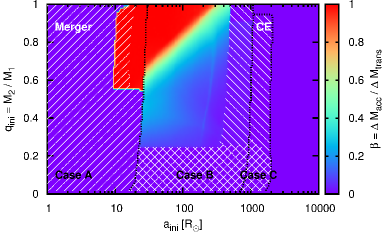
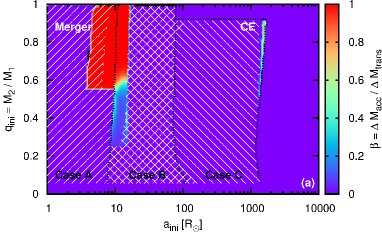
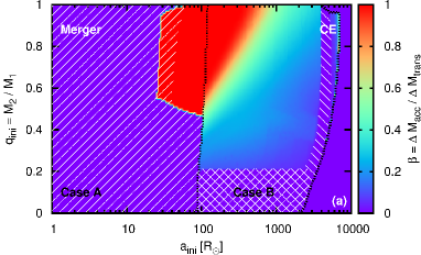
In Fig. 1 we show the mass transfer efficiency $\beta$ (Eq. 8) in binaries with $10\,{\rm M}_{\odot}$ primary stars as a function of initial mass ratio, $q_{\mathrm{ini}}$, and initial orbital separation, $a_{\mathrm{ini}}$. Binaries interact by Case A mass transfer if the initial orbital separation is less than about $20$-$30\,{\rm R}_{\odot}$. They first interact by Case B mass transfer if the initial orbital separation is longer than the boundary for Case A mass transfer and shorter than $800$–$1000\,{\rm R}_{\odot}$. They first interact by Case C mass transfer if the initial orbital separation is longer than $800$–$1000\,{\rm R}_{\odot}$. They do not interact by RLOF at all if the initial orbital separation is longer than about $2000\,{\rm R}_{\odot}$. The boundaries depend on the initial mass ratio: if the mass ratio is larger (for a fixed orbital separation), the primary overflows its Roche lobe earlier in its evolution because the Roche lobe is smaller. The boundaries between the different mass transfer cases therefore shift to longer initial orbital separations for larger mass ratios.

There is a small zone/gap above the Case C mass transfer region for large initial mass ratios ($q\gtrsim 0.95$) where stars interact by Case C mass transfer, but only after the secondary has left the MS, hence the gap.

In Fig. 1, we also mark those binaries as mergers which start RLOF on the ZAMS (we do not treat these binaries in our simulations). We assume that stars enter a contact phase if their mass ratio at the onset of Case A mass transfer is less than $0.56$ (Sec. 2.1). Only the products of these Case A mergers are MS stars and only these contribute to our analysis of the PDMF.

There are two more critical mass ratios visible in Fig. 1: we assume that stars enter common envelope evolution at the onset of Case B RLOF if the donor star is a Hertzsprung gap star and the mass ratio is below $0.25$. For giant-like donor stars, i.e. donor stars with a deep convective envelope (e.g. red supergiants), we use a formula (Eq. 57 in Hurley et al. 2002) to calculate the critical mass ratio. Mass loss from a star with a deep convective envelope leads to an increase of its radius, hence to even more mass transfer and is thus dynamically unstable. The giant-like donor star engulfs its companion and the binary enters common envelope evolution. If all these criteria do not apply for the binary star at the onset of RLOF we use the critical mass ratio $q_{\mathrm{c}}=0.33$.

Figure 2.— The mass $\Delta M_{\mathrm{trans}}$ transferred from $10\,{\rm M}_{\odot}$ donor stars by RLOF during the MS evolution of the secondary star as a function of the initial mass ratio and the initial orbital separation. The hatched regions have the same meaning as in Fig. 1.

Figure 3.— As Fig. 2 but for the total mass accreted by the secondary star, $\Delta M_{\mathrm{acc}}$, during RLOF.

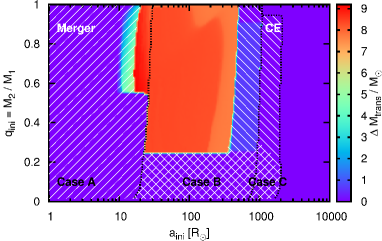
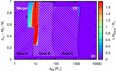
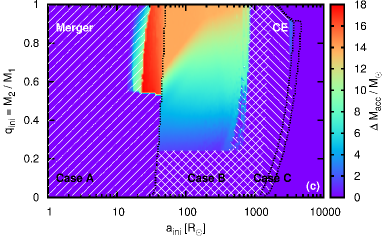
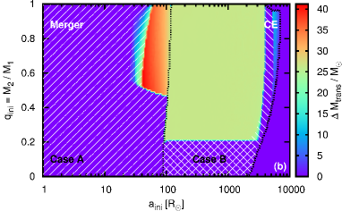
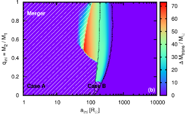
The transferred mass $\Delta M_{\mathrm{trans}}$ from a $10\,{\rm M}_{\odot}$ primary star during RLOF is shown in Fig. 2. The transferred mass is very similar in all interacting binaries that do not enter a contact phase Case A mass transfer is caused by increasing stellar radii due to nuclear evolution during core hydrogen burning. MS stars with masses larger than $1.25\,{\rm M}_{\odot}$ have radiative envelopes in our models. Mass transfer from stars with radiative envelopes is stable, i.e. such stars shrink back into their Roche lobe as a reaction to mass loss. Case A RLOF starts earlier and lasts longer for smaller initial orbital separations, hence the smaller the initial orbital separation the larger the mass lost by the donor, i.e. the transferred mass $\Delta M_{\mathrm{trans}}$. During Case B and C mass transfer, RLOF is driven by the expansion of the stellar envelope. Stars stop overfilling their Roche lobes only after losing (nearly) their whole envelope. The envelope mass of the $10\,{\rm M}_{\odot}$ donor stars of the Case B binaries which do not enter a CE evolution is always about the same, hence is the total transferred mass in Fig. 2.

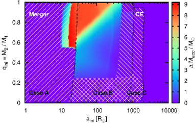
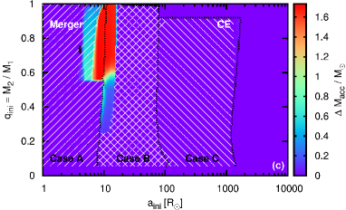
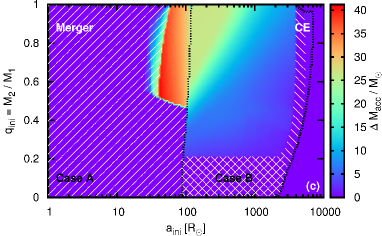
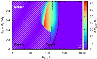
Figure 3 shows how much of the mass transferred from the $10\,{\rm M}_{\odot}$ donor stars is accreted by the secondary stars during their MS evolution. The only limit on mass accretion in our models is the thermal timescale of the accretor which ensures that the accretors remain in thermal equilibrium, an implicit assumption when using fitting functions for single star evolution. The thermal (Kelvin-Helmholtz) timescale is given by

$$\tau_{{\rm KH}}\approx 10^{7}\frac{M/{\rm M}_{\odot}M_{\mathrm{env}}/{\rm M}_{\odot}}{R/{\rm R}_{\odot}L/{\rm L}_{\odot}}\,\mathrm{yr},$$ (9)

where $M$ is the total mass, $M_{\mathrm{env}}$ the mass of the envelope ($M_{\mathrm{env}}=M$ for MS stars), $R$ the radius and $L$ the luminosity of the star. Nearly all transferred mass is accreted during Case A mass transfer. Mass transfer during the Hertzsprung gap, i.e. Case B mass transfer, proceeds on the thermal timescale of the primary. At longer initial orbital separations, the thermal timescale of the primary is shorter because the primaries have larger radii when they overfill their Roche lobes (mass and luminosity are nearly constant in the Hertzsprung gap). The thermal timescale of the MS secondary at the same time is inversely proportional to a power of its mass ($\tau_{\mathrm{KH}}\propto M^{-x}\,,x>0$). We therefore expect less accretion at longer initial orbital separations (because of shorter thermal timescales of the donor stars and hence faster mass transfer) and for smaller initial secondary masses (because of longer thermal timescales of less massive accretors). This causes the gradient visible in the Case B region of Figs. 1 and 3.

Combining the results of the transferred and accreted mass during RLOF reveals the mass transfer efficiency as shown in Fig. 1. Mass transfer is nearly conservative during Case A, i.e. almost all transferred mass is accreted ($\beta\approx 1$), and becomes non-conservative during Case B and C mass transfer.

Figure 4.— Fraction of simulated binaries that interact by RLOF during the MS of the secondary stars and fraction of interacting binaries that merge on the MS, that transfer mass stably by RLOF and that go through a common envelope (CE) phase as a function of the mass of the primary stars. The number of simulated binaries is given by $N_{\mathrm{simulated}}$, the number of interacting binaries by $N_{\mathrm{interact}}$, the number of binaries that merge on the MS by $N_{\text{MS merger}}$, the number of binaries that transfer mass stably by RLOF by $N_{\text{stable RLOF}}$ and the number of binaries that go through a CE phase by $N_{\mathrm{CE}}$. By interacting binaries, we mean that the primary overfills its Roche lobe resulting in mass transfer or a merger.

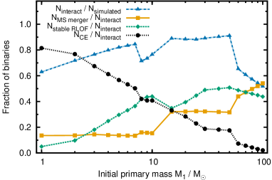
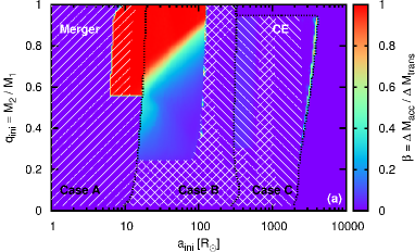
Next, we analyse the binary parameter space for different primary masses. Figures 17–22 in Appendix A contain the mass transfer efficiency, transferred and accreted mass as in Figs. 1, 2 and 3 but for primary masses of $2$, $5$, $20$, $50$, $70$ and $100\,{\rm M}_{\odot}$. Binaries in which the primary star once filled its Roche lobe are called interacting binaries. From the data of Fig. 1, we compute the ratios of the number of binaries that go through a common envelope phase, merge on the MS and transfer mass stably by RLOF to the number of interacting binaries and the ratio of the number of interacting to simulated binaries. We plot these ratios as a function of primary mass in Fig. 4 taking into account the initial distribution functions of binaries discussed in Sec. 2.2. The overall trend is that the more massive the primary star the larger the fraction of stars that transfer mass stably by RLOF, the larger the fraction of stars that merge on the MS and hence the smaller the fraction of binaries that go through a common envelope phase.

The number of interacting binaries decreases rapidly around $50\,{\rm M}_{\odot}$ because more massive stars cross the Humphreys–Davidson limit (Humphreys & Davidson 1979) after their MS evolution and are subject to strong wind mass loss. The mass loss widens the orbits such that binaries cannot interact by RLOF (cf. Vanbeveren 1991). Consequently, the fraction of MS mergers increases because it is normalized by the number of interacting binaries while the number of Case B binaries that go through a common envelope phase ($q_{\mathrm{ini}}<0.25$) decreases.

The fraction of interacting binaries shows a kink around $8\,{\rm M}_{\odot}$ because this is the mass above which stars explode as supernovae. Our $7\,{\rm M}_{\odot}$ model reaches a maximum radius that is larger than that of e.g. our $8\,{\rm M}_{\odot}$ model because the latter star explodes before reaching a similarly large radius. The parameter space for interaction is therefore smaller in binaries with $8\,{\rm M}_{\odot}$ primary stars. From thereon, the number of interacting binaries gradually increases with primary mass because more massive primary stars reach larger maximum radii. Above $\sim 13\,{\rm M}_{\odot}$, the maximum radius is larger than that of a $7\,{\rm M}_{\odot}$ star and so is the fraction of interacting binaries.

Between $2$ and $10\,{\rm M}_{\odot}$ the fraction of binaries that transfer mass stably by RLOF increases while the fraction of systems that go through a common envelope phase decreases. Stars more massive than about $2\,{\rm M}_{\odot}$ expand significantly while crossing the Hertzsprung-Russell diagram and the chance of interaction by Case B mass transfer is therefore larger. Less massive stars are cooler and develop convective envelopes, ascending the giant branch (GB), after little expansion. Mass transfer from such stars is dynamically unstable leading to a common envelope phase. The more massive stars are, the larger the Hertzsprung gap, the larger the number of stars that interact by Case B mass transfer while having a radiative envelope and the fewer the number of binaries that enter a common envelope phase.

Stars with $M\gtrsim 13\,{\rm M}_{\odot}$ ignite helium in the core during the Hertzsprung gap in our models and only slightly climb the GB, meaning there is only a limited range of initial orbital separations that leads to stars that interact as giants and thus enter a common envelope phase. Contrarily, the fraction of binaries that transfer mass stably by RLOF plateaus for primary masses greater than $10\,{\rm M}_{\odot}$ because the available range of separations to transfer mass from a star without a fully convective envelope does not change significantly.

Binaries in which the primary star is more massive than about $22\,{\rm M}_{\odot}$ do not experience Case C mass transfer because the primary stars lose their envelopes through strong stellar winds during core helium burning which widens the orbit and prevents the star from further expansion. As a consequence, the star cannot overfill its Roche lobe after core helium burning and there is no Case C mass transfer.

Binaries with O-type primaries, i.e. with $M_{1}\geq 15\,{\rm M}_{\odot}$ are distributed according to the initial orbital period distributions of Sana et al. (2012). This enhances the number of stellar mergers on the MS and the occurrence of Case A mass transfer because there are more binaries with short orbital periods according to the orbital period distribution of Sana et al. (2012) than for a distribution that is flat in $\log P$ as used for less massive stars. The change of the period distribution leads to the abrupt increase in the fraction of MS mergers around $15\,{\rm M}_{\odot}$ and the decrease of the fraction of binaries transferring mass stably by RLOF because the emphasis is now on binaries in the closest orbits which preferentially merge (see Figs. 1 and 17–22).

We discuss uncertainties in our models regarding single and binary star evolution and the initial distribution functions in Appendix B.

2.4. Construction of mass functions

Constructing the mass function of a population of single stars is straightforward: we bin the masses and count the number of stars per mass bin. In the case of binary stars we construct three different mass functions according to:

1. The primary masses only.

2. The secondary masses only.

3. An observed mass reconstructed from the total stellar luminosity.

In the latter case we derive masses from the total luminosity of binaries: we add the luminosities of both components and numerically invert the mass-luminosity (ML) relation given by our fitting formula (Eq. 12 of Hurley et al. 2000). We call mass functions constructed in this way observed mass functions, because it comes closest to mass functions from photometry where luminosities are directly translated into masses and binaries are unresolved. We emphasize again that we only consider MS stars in our analysis.

3. Modulation of mass functions by stellar evolution

3.1. Single star populations

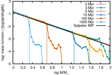
Two phenomena influence the mass functions of a population of single stars. First, stars have shorter lives the more massive they are. When stars leave the MS, they disappear from our mass functions. Second, massive stars lose mass through stellar winds. This reduces stellar masses and hence changes the mass function. In Fig. 5 we show PDMFs of coeval single star populations of different ages. The mass functions are constructed from the theoretically known stellar masses (approach 1 in Sec. 2.4). The dashed vertical lines mark the initial mass of stars that have a MS lifetime equal to the age of the population. Over-plotted in black is the initial distribution of stellar masses, i.e. the Salpeter (1955) IMF.

Figure 5.— Present-day mass functions of coeval single star populations of different ages. Dashed vertical lines correspond to the mass of stars with a MS lifetime equal to the age of the population. The most massive stars have the shortest MS lifetime and hence disappear first. Stellar wind mass loss creates the peaks at the high mass end most prominently seen in the $3.0\,{\rm Myr}$ old population.

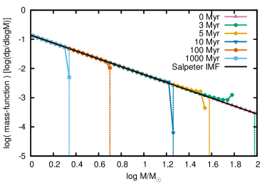
The most massive stars leave the MS first which causes a truncation close to the dashed vertical lines. From here on we call this truncation the turn-off because stars at the truncation of the mass function are located at the turn-off in the Hertzsprung–Russell (HR) diagram of a star cluster. Stars at the turn-off are called “turn-off stars” and their mass the “turn-off mass”. Younger than about $10\,{\rm Myr}$ the turn-off and the dashed lines do not coincide, they are displaced from each other. The displacement is caused by stellar wind mass loss and amounts to $\sim 40\,{\rm M}_{\odot}$ in the $3.0\,{\rm Myr}$ PDMF for our adopted mass loss recipes.

We use a maximum initial stellar mass of $100\,{\rm M}_{\odot}$. Such stars have MS lifetimes of about $3.0\,\mathrm{Myr}$, so the upper mass boundary plays no role in populations older than $3.0\,\mathrm{Myr}$ because all stars with initially masses larger than $100\,{\rm M}_{\odot}$ have left the MS. Our results are influenced by boundary effects at ages younger than $3.0\,\mathrm{Myr}$.

A prominent feature in the PDMF is the accumulation of stars close to the turn-off because of mass loss through stellar winds. The more massive a star the more mass is lost during its MS evolution. Stars with masses close to the turn-off mass are the currently most massive stars in the cluster and will soon leave the MS, so the greatest accumulation of stars in the PDMF is found close to the turn-off. In our calculations, stars initially less massive than $9\,{\rm M}_{\odot}$ at $Z=0.02$ ($\tau_{\mathrm{MS}}\gtrsim 30\,\mathrm{Myr}$) lose less than $1\%$ of their initial mass via winds during the MS — the accumulation of stars in the PDMF disappears totally and the initial and the present-day turn-off masses are the same (the dashed vertical lines coincide with the turn-off). Note that we do not see a sharp truncation as indicated by the dashed vertical lines because of the finite size of our mass bins.

Figure 6.— High mass end ($\geq 10\,{\rm M}_{\odot}$) of mass functions of coeval stellar populations with IMF slopes $\Gamma$ and metallicities $Z$. The panels show (a) a population drawn from a Salpeter IMF $\Gamma=-1.35$ at solar metallicity $Z=0.02$, (b) as (a) with $Z=0.01$, (c) as (a) with $\Gamma=-0.9$ and (d) as (c) with $Z=0.01$. The black dotted line shows the IMF and the filled regions labelled $N_{1}$ indicate the accumulation of stars because of stellar wind mass loss at an age of $3\,{\rm Myr}$. Because the area labelled $N_{1}$ contains those stars that depopulated the mass function for masses beyond the mass function peak, it contains the same number of stars as the area labelled $N_{2}$. The wind mass loss peaks are stronger the flatter, i.e. the more positive, the IMF slope and the stronger the wind mass loss (i.e. the higher the metallicity).

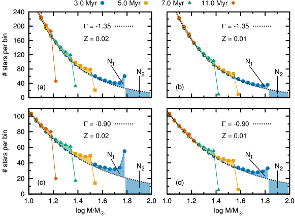
The magnitude of the wind mass loss peak in the PDMF depends on how many stars are shifted to lower masses and by how much. It therefore depends on the strength of stellar wind mass loss, i.e. also on the metallicity, and the slope of the IMF. In Fig. 6 we show this dependence at the high mass end of PDMFs ($\geq 10\,{\rm M}_{\odot}$) on a linear scale where the size of the bump is more apparent: the higher the metallicity, i.e. the stronger the wind mass loss, the bigger the peak. Similarly, the flatter the mass function, i.e. the more high mass stars exist compared to lower mass stars, the bigger the peak. The number of stars in the highest-mass bin of the $3\,{\rm Myr}$ mass function is increased compared to the IMF by $127\%$ for $\Gamma=-1.35$ and by $162\%$ for $\Gamma=-0.9$ at a metallicity $Z=0.02$ and by about $55\%$ for $\Gamma=-1.35$ and $70\%$ for $\Gamma=-0.9$ at $Z=0.01$.

The wind mass loss peak allows us to determine the overall mass lost by stars during their MS evolution. In practice, it may be necessary to model luminosity functions rather than mass functions with different mass loss recipes to match observed luminosity functions. Only by doing so can one overcome the inherent problem that masses derived from observed luminosities rely implicitly on the mass loss prescription used to derive the applied ML relations.

Figures 5 and 6 show that the wind mass loss peak is only visible in sufficiently young clusters in which stellar winds are strong. We now investigate the age and metallicity range of stellar populations whose mass functions are likely to show the wind mass loss peak. Let $M_{{\rm to,p}}$ be the present-day turn-off mass in the star cluster and $N_{1}$ the number of excess stars in the peak compared to the IMF which is a power-law with slope $\Gamma$ (Eq. 4). We can then redistribute these stars such that the peak is removed by filling up the IMF from the top end, thereby obtaining the initial mass of the turn-off stars, $M_{{\rm to,i}}$. Let $\Delta M$ be the mass lost by turn-off stars over their MS evolution, i.e. $\Delta M=M_{\mathrm{to,i}}-M_{\mathrm{to,p}}$. Because the number of excess stars $N_{1}$ equals the number of stars $N_{2}$ between $M_{{\rm to,p}}$ (Fig. 6), we have,

$$N_{1}=N_{2} =\int_{M_{{\rm to,p}}}^{M_{{\rm to,p}}+\Delta M}\,\psi(M)\,{\rm d}M=N_{2}$$ (10)

$$=\frac{A}{\Gamma}M_{\mathrm{to,p}}^{\Gamma}\left[\left(1+\frac{\Delta M}{M_{\mathrm{to,p}}}\right)^{\Gamma}-1\right].$$

To judge whether the accumulation of $N_{1}$ stars is enough to see a wind mass loss peak, we have to compare $N_{1}$ to the number of stars expected from the IMF in a mass range that is slightly less massive than the turn-off, $N_{\mathrm{imf}}$. We define $N_{\mathrm{imf}}$ to be the number of stars in the mass range from $fM_{\mathrm{to,p}}$ to $M_{\mathrm{to,p}}$ where $f<1$. For $f=0.75$, we require that $N_{1}$ has to exceed 10% of $N_{\mathrm{imf}}$ to be able to see the wind mass loss peak. The 10% requirement and the value for $f$ are chosen such that a visible wind mass loss peak is predicted in the $7\,\mathrm{Myr}$ but not $11\,\mathrm{Myr}$ stellar populations at $Z=0.01$ and $Z=0.02$ (cf. Fig. 6). Analogously to Eq. (10), we compute $N_{\mathrm{imf}}$ and find that,

$$\frac{N_{1}}{N_{\mathrm{imf}}}=\frac{\left(1+\Delta M/M_{\mathrm{to,p}}\right)^{\Gamma}-1}{1-f^{\Gamma}}>10\%\;\mathrm{for}\;f=0.75$$ (11)

in order for the wind mass loss peak to be visible. This criterion translates into a relative wind mass loss of,

$$\frac{\Delta M}{M_{\mathrm{to,p}}}\geq\left[\frac{N_{1}}{N_{\mathrm{imf}}}\left(1-f^{\Gamma}\right)+1\right]^{1/\Gamma}-1.$$ (12)

According to our criterion, the minimum relative mass loss is 3.7% for $\Gamma=-1.35$ and 3.3% for $\Gamma=-0.7$.

Figure 7.— Fractional initial mass loss, $\Delta M/M_{\mathrm{ini}}$, of stars during the main sequence as a function of initial mass and metallicity $Z$. The solid and dotted lines show the criterion of the visibility of the wind mass loss peak in mass functions from Eq. (11) for $N_{1}/N_{\mathrm{imf}}=5$, 10 and 15%, respectively, and an IMF slope of $\Gamma=-1.35$. According to our criterion, a wind mass loss peak is likely visible in stellar populations to the right of the solid, 10% line (see text for more details).

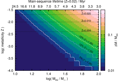
In Fig. 7, we show how much mass is lost by stars through stellar winds during their MS evolution as a function of initial mass and metallicity. We further indicate the corresponding MS lifetimes for $Z=0.02$ on the top and plot the criterion from Eq. 11 for $N_{1}/N_{\mathrm{imf}}=5$, 10 and 15%. The mass functions of stellar populations of ages and metallicities to the right of the $N_{1}/N_{\mathrm{imf}}=10\%$ line are likely to show the wind mass loss peak. As a rule of thumb, the mass functions of stellar populations younger than about $10\,\mathrm{Myr}$ at $Z=0.02$ are likely to show a visible wind mass loss peak. Note that our criterion is a rather rough estimate and depends on the wind mass loss prescription and its metallicity scaling.

3.2. Binary star populations

Two processes additionally influence the mass functions of binary star populations compared to those of single stars. First, stars can merge during their evolution and, second, stars can accrete mass by RLOF. In what follows we discuss three different mass functions to disentangle these effects: we present mass functions of primary stars, of secondary stars and those constructed from the ML inversion method (observed mass functions) as discussed in Sec. 2.4.

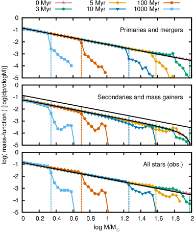
The primary star is initially more massive than the secondary star, so it evolves faster and is the donor star during RLOF. Analogously, the secondary star is the mass gainer. In the top panel of Fig. 8 we show the mass functions of primary stars, i.e. stars that have not yet interacted, that have lost mass by mass transfer or that have merged. The mass functions in the middle panel of Fig. 8 show secondary stars that have not interacted yet and that have gained mass by RLOF. The observed mass function in the bottom panel of Fig. 8 is a combination of all stellar evolutionary effects.

Figure 8.— Temporal evolution of PDMFs of all primary stars and mergers (top panel), all secondary stars (middle panel) and for observed masses for all stars (bottom panel; see Sec. 2.4). By construction, merged stars appear in the PDMFs in the top panel and mass gainers of RLOF in the PDMFs in the middle panel. The vertical dashed lines indicate the mass of stars having a MS lifetime equal to the age of the population, i.e. they indicate the initial mass of the turn-off stars. Contrary to a population made only of single stars, stars more massive than the initial mass of the turn-off stars exist. The black solid lines are the Salpeter IMF and the initial distribution function of the secondary stars (Eq. 13) respectively.

The primary stars are initially distributed according to the Salpeter IMF (Eq. 4) and the secondary stars according to

$$\frac{{\rm d}p}{{\rm d}\ln m_{2}} = \int_{\ln m_{2}}^{\ln 100}\psi(\ln m_{1})\phi(\ln m_{2})\,\mathrm{d}\ln m_{1}\cdot\underbrace{\int_{\ln a}\chi(\ln a)\,\mathrm{d}\ln a}_{=1}$$ (13)

$$\approx \frac{A}{\Gamma-1}m_{2}\left(100^{\Gamma-1}-m_{2}^{\Gamma-1}\right),$$

where $\psi(\ln m_{1})$, $\phi(\ln m_{2})$ and $\chi(\ln a)$ are the initial distribution functions of the primary and secondary masses and the orbital separations as defined in Sec. 2.2 (we assume $q_{\mathrm{min}}\approx 0.0$ in the last step). Compared to the IMF of primary stars, the initial mass distribution of secondary stars is lowered by a factor $(1-\Gamma)^{-1}$ ($\approx 0.43$). The decline of the secondary IMF at the high mass end is caused by the maximum initial mass (cf. the first term on the right-hand side of Eq. 13: the maximum initial mass in our calculations is $100\,{\rm M}_{\odot}$). The overall slope is $\Gamma=-1.35$ again because of the flat mass ratio distribution.

In single stars, no star is more massive than the turn-off. Including binary stars it is possible to populate a tail of stars that extends the high mass end of single star PDMFs by about a factor of 2 in mass.

In the top panel of Fig. 8 only stellar mergers populate the PDMF tail (i.e. the PDMF on the right-hand side of the vertical dashed lines). The relative number of mergers in the tail is lower the older the population as expected from our analysis of the binary parameter space in which the fraction of binary stars that merge on the MS increases with the initial mass of the primary star (Fig. 4).

The maximum mass of stellar mergers is reached by initially equal-mass binaries in which the final mass is the total mass of the binary minus a fraction of 10% that we assume is lost during a merger (Sec. 2.1). This corresponds to a mass increase by a factor of $1.8$ or a shift of about $0.26\,\mathrm{dex}$ on the logarithmic mass scale. The PDMF at $10\,\mathrm{Myr}$ extends slightly further because of the rejuvenation of the merged stars. The mass of the merged star is not increased by more than a factor of $1.8$ relative to the primary mass, but fresh hydrogen is mixed into its core. This decreases the fraction of burnt fuel and hence the apparent age of the star. Compared to genuine single stars of comparable mass, i.e. stars which have not interacted, the stellar merger has more available fuel and thus stays longer on the MS. Rejuvenated stars can thus appear to be shifted by more than $0.26\,\mathrm{dex}$ because the turn-off mass decreases simultaneously.

The PDMF tails in the middle panel of Fig. 8 contain secondary stars that have accreted mass. The PDMFs again extend to slightly larger masses than expected from mass accretion alone because of rejuvenation. Mass accretion in young stellar populations (ages $\lesssim 10\,\mathrm{Myr}$) forms PDMF tails that even exceed the initial distribution of the secondary stars. At later times, the relative number of stars in the tail is less because the number of interacting binaries that transfer mass stably by RLOF decreases for initially less massive primary stars (Fig. 4) as does the overall mass transfer efficiency, $\beta$, which is coupled to the thermal timescale of the mass gainers during Case B mass transfer. The thermal timescales of stars become more comparable for larger masses because the ML and mass-radius relations are less steep the larger the mass.

In populations younger than $3.0\,{\rm Myr}$, the effect of mass accretion on the PDMF is modest because the most massive stars in our models have just left the MS and hence there is no contribution from Case B mass transfer to the PDMF (Case C does not occur for primary masses larger than about $22\,{\rm M}_{\odot}$, see Sec. 2.3). The number of interacting binaries drops strongly for primary masses larger than about $50\,{\rm M}_{\odot}$ because of the Humphreys–Davidson limit (Sec. 2.3). This is important in stellar populations younger than $\sim 4.3\,\mathrm{Myr}$ which is the MS lifetime of $50\,{\rm M}_{\odot}$ stars in our models.

In the bottom panel of Fig. 8 we use the ML inversion method (approach 3 in Sec. 2.4) to construct the PDMFs. Both, mergers and accretors show up in the PDMF tails. The star with the highest mass in each population is formed by RLOF. However, the difference between the highest mass achieved by stellar mergers and by RLOF is small — at most one bin-width, i.e. $\Delta\log m=0.04\,{\rm dex}$ — and depends on the assumed mass loss in stellar mergers and the mass transfer efficiency. Only at early times ($\lesssim 3.5\,\mathrm{Myr}$) does the star with the highest mass originate in a stellar merger. Unresolved binaries also contribute to the tail of the observed PDMFs but their contribution is small (at most $30\%$ of the tail stars are unresolved binaries in young, $\lesssim 3$–$4\,\mathrm{Myr}$ populations) and greatest for the largest masses because of a flatter ML relation of high mass stars compared to lower masses. Unresolved binaries extend the single star mass function by at most $\sim 20\%$ in mass for $1\dots 2\,{\rm M}_{\odot}$ stars and by at most $\sim 50\%$ in mass for $60\dots 100\,{\rm M}_{\odot}$ stars (cf. Eq. 15 in Sec. 3.4).

Figure 9.— Mass functions at $5$, $20$ and $100\,\mathrm{Myr}$ for secondary stars, i.e. mass accretors. The curves show the contributions of the mass transfer Cases A, B and C (as defined in Sec. 2.1) to the total PDMF of secondaries (black squares). Case B mass transfer is the dominant contribution to the tail stars for $\gtrsim 3\,\mathrm{Myr}$, hence the mass loser is not a MS star and therefore not present in the PDMFs of primaries in the top panel of Fig. 8. This is why the mass gainers are seen clearly in the PDMFs whereas the mass losers are not.

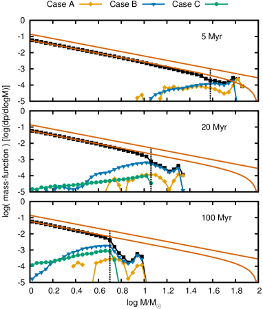
In Fig. 9 we show the PDMF of secondary stars at three different times — $5$, $20$ and $100\,\mathrm{Myr}$. Case B mass transfer is the dominant contribution after $3\,\mathrm{Myr}$, therefore the mass losing star has left the MS and is no longer included in the PDMFs of the primary stars in the top panel of Fig. 8. The Case A mass losers are difficult to find. Nevertheless some of them can be found by comparing the PDMFs of populations of single (Fig. 5) and binary stars only (top panel of Fig. 8). The mass losers are easiest to spot by the difference in the magnitude of the accumulation of stars because of wind mass loss e.g. in the PDMFs of the $5\,{\rm Myr}$ old populations. Populations made only of single stars show a larger accumulation of stars than those made of binary stars, because some donor stars that would appear in the wind mass loss peak lose additional mass during Case A mass transfer. In practice it is very hard to detect the primaries after they have lost mass (de Mink et al. 2014).

Case C mass transfer is typically highly non-conservative in our models (Sec. 2.3 and Appendix A). The secondary stars of such systems therefore do not gain enough mass to make any significant contribution to the tail.

The stars in the tail of the mass functions are rejuvenated binary products and hence appear younger than the real age of the population — they are blue stragglers. We further characterise these blue straggler stars in Sec. 4 in terms of their binary fraction and apparent ages and compare their frequencies to observations.

3.3. Stellar populations with varying binary fractions

We use the PDMFs of populations of single and binary stars presented in Secs. 3.1 and 3.2 to build stellar populations composed of a mixture of coeval single and binary stars. Let $f_{\mathrm{B}}$ be the binary fraction at birth, i.e. the number of binary systems divided by the number of total stellar systems ($f_{\mathrm{B}}=N_{\mathrm{B}}/[N_{\mathrm{S}}+N_{\mathrm{B}}]$ with $N_{{\rm B}}$ the number of binary systems and $N_{{\rm S}}$ the number of single stars). The considered binaries have initial orbital separations shorter than $10^{4}\,{\rm R}_{\odot}$ — initially wider binaries are treated as single stars in our models (Sec. 2.2). The mass function of a population with this binary fraction is then,

$$\frac{\mathrm{d}p}{\mathrm{d}\log m}=(1-f_{\mathrm{B}})\cdot\left(\frac{\mathrm{d}p}{\mathrm{d}\log m}\right)_{\mathrm{s}}+f_{\mathrm{B}}\cdot\left(\frac{\mathrm{d}p}{\mathrm{d}\log m}\right)_{\mathrm{b}}.$$ (14)

Here $\left(\mathrm{d}p/\mathrm{d}\log m\right)_{\mathrm{s}}$ is the mass function of single stars only and correspondingly $\left(\mathrm{d}p/\mathrm{d}\log m\right)_{\mathrm{b}}$ is the mass function of binary stars only. In Fig. 10 we show the observed mass functions of stellar populations with a primordial binary fraction of $f_{\mathrm{B}}=0.5$ (i.e. two out of three stars initially born in binaries). In comparison to Fig. 8, the number of stars in the binary tail in the PDMFs (Sec. 3.2) is attenuated. The tail of the mass functions of stellar populations with a binary fraction of 50% is decreased by $0.3\,\mathrm{dex}$, i.e. by a factor of 2, compared to those with a binary fraction of 100%.

Figure 10.— As the bottom panel of Fig. 8, but for a population of stars with a primordial binary fraction of $f_{\mathrm{B}}=0.5$. As discussed in Sec. 3.3 the number of stars in the binary tails are halved compared to a pure binary star population.

3.4. Quantification of evolutionary effects on the PDMF

Figure 11.— Slopes of the PDMF of single stars (Sec. 3.1) as a function of logarithmic mass. Stellar wind mass loss flattens the high mass end of the PDMFs.

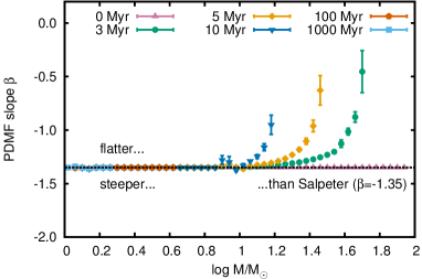
The stellar wind mass-loss peak at the high mass end flattens the mass function. We quantify the flattening by computing the PDMF slopes as a function of stellar mass. We fit straight lines piecewise to three mass bins at a time by a Levenberg–Marquardt method (Levenberg 1944; Marquardt 1963) and show the slopes $\beta$ of the single star PDMFs in Fig. 11. The errors are statistical $1\sigma$ deviations from the best fit. The more massive a star the more mass is lost by stellar winds, hence the accumulation and resulting flattening of the PDMF is strongest in the $3\,\mathrm{Myr}$ population. The slope at the high mass end of the mass function of young stellar populations ($\lesssim 10\,\mathrm{Myr}$) is much shallower than the Salpeter IMF, $\Gamma=-1.35$. We find extremes of the PDMF slope of $\beta\approx-0.45\pm 0.20$ at the highest masses around $50\,{\rm M}_{\odot}$ ($\log M/{\rm M}_{\odot}\approx 1.7\,{\rm dex}$) in the $3\,{\rm Myr}$ population. The flattening is still significant for $10\,\mathrm{Myr}$ populations at masses more than $10\,{\rm M}_{\odot}$ for which the slope flattens to values of up to $\beta\approx-0.95\pm 0.09$. In other words, not accounting for wind mass loss when determining the slope of the IMF for the most massive stars may lead to IMF slopes that are biased by up to 1 dex.

We further quantify the wind mass loss peak and the binary tail by dividing the PDMFs of populations consisting purely of single stars, purely of binary stars and of a mixture of single and binary stars by the initial distribution functions (Eqs. 4 and 13) in order to determine the relative importance of the evolutionary effects compared to the initial distribution of stellar systems. First, we construct PDMFs from the theoretically known stellar masses and not using the ML inversion method and show the ratio of PDMF to IMF in Fig. 12. This enables us to distinguish between the effects of single and binary star physics and of unresolved binaries on the PDMF. Again, the truncations of the PDMFs are due to finite stellar lifetimes.

Figure 12.— Ratio of the PDMFs to IMFs for different ages and primordial binary fractions. The PDMFs are constructed from the known stellar masses (approaches 1 and 2 in Sec. 2.4).

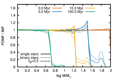
The PDMF of the $5\,{\rm Myr}$ single star population reaches a level of more than $120\%$ of the IMF because of an accumulation of stars caused by wind mass loss (blue solid line close to the turn-off mass of $\log m\approx 1.5\,{\rm dex}$). The wind mass loss peak becomes weaker with age until it completely disappears in stellar populations older than $30\,\mathrm{Myr}$ (at a metallicity of $Z=0.02$ with a Salpeter IMF; see also Sec. 3.1).

Stellar mergers and mass transfer by RLOF shift stars toward higher masses. The number of stars that are slightly less massive than the turn-off stars is therefore less than the initial number of stars, i.e. $\mathrm{PDMF}/\mathrm{IMF}<1$ (with no wind mass loss). The tail of the $5\,{\rm Myr}$ binary population reaches an average level of more than $30\%$ of the initial distribution function, i.e. on average about one third of the IMF in a mass range from about $40\,{\rm M}_{\odot}$ ($\log m\approx 1.6\,{\rm dex}$) to $80\,{\rm M}_{\odot}$ ($\log m\approx 1.9\,{\rm dex}$) is re-populated by binary evolution. This level gradually decreases the older the population and the smaller the binary fraction.

Figure 13.— As Fig. 12 but constructed using the mass-luminosity inversion method (approach 3 in Sec. 2.4).

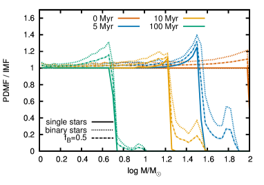
Being unable to resolve binaries shifts the observed mass function to larger masses (Fig. 13). This is well known (Sagar & Richtler 1991; Kroupa et al. 1993; Maíz Apellániz 2008; Weidner et al. 2009) and is evident from the initial mass distribution of pure binary star populations ($0\,{\rm Myr}$ binary population in Fig. 13). In a single star population there is no difference between the observed IMF and the Salpter IMF. With unresolved binaries, the PDMF exceeds the IMF and the ratio of PDMF to IMF increases with larger binary fractions. In stellar populations with $f_{\mathrm{B}}=0.5$ there are $5-10\%$ more stellar systems than expected from the Salpeter IMF and up to $\sim 20\%$ more for pure binary populations ($f_{\mathrm{B}}=1$). The increase is mass dependent: it is greater for larger masses and is understood from the ML relation, which can be approximated as $L=L_{0}M^{x}$. In unresolved binaries with equal masses $M$ the observed mass $M_{\mathrm{obs}}$ is

$$M_{\mathrm{obs}}=\left(\frac{L_{1}+L_{1}}{L_{0}}\right)^{1/x}=2^{1/x}M,$$ (15)

i.e. larger than $M$ by a factor of $2^{1/x}$. Low mass stars have a larger exponent $x$ than high mass stars, hence the larger the mass $M$ the larger the factor by which the observed mass is increased (e.g. $L\propto M^{4.5}$ for $1\leq M/{\rm M}_{\odot}\leq 2$ and $L\propto M^{1.8}$ for $60\leq M/{\rm M}_{\odot}\leq 100$ ZAMS stars, Tout et al. 1996). This translates into an increase of the mass function by a factor of

$$\frac{\psi(\ln M)}{\psi(\ln M_{\mathrm{obs}})}=2^{-\Gamma/x}=1.23\dots 1.68,$$ (16)

where $\Gamma$ is the IMF slope. Unresolved binaries flatten the PDMF most strongly at the largest stellar masses (under the assumption that $\Gamma$ is constant in the considered mass range). We discuss the effect of unresolved binaries on mass functions with respect to previous work in more detail in Appendix C.

Figure 13 shows that unresolved binaries flatten the PDMF at masses less than the turn-off mass instead of steepening the PDMF as was the case for resolved binaries. The wind mass-loss peaks in the PDMF reach a level of up to $\sim 140\%$ of the IMF. The tail of the $5\,{\rm Myr}$ binary population is re-populated by on average $\gtrsim 40\%$ and with maximum levels of about $55\%$ of the IMF. The number of stars in the binary tail is halved in populations with a binary fraction of $f_{\mathrm{B}}=0.5$.

We have shown above that stellar wind mass loss, binary products and unresolved binaries re-shape the high mass end of mass functions which may complicate IMF determinations. To avoid biased IMF slope determinations in young as well as old clusters, we suggest to either exclude those parts of the mass function that are expected to be affected by stellar winds, binary products and/or unresolved binaries or to correct for these effects. As evident from Fig. 13, this concerns roughly the mass ranges from $0.5\text{--}0.6$ to twice the turn-off mass in our models (about $\pm 0.3\,\mathrm{dex}$ around the turn-off).

4. Blue straggler stars

The stars in the tail of mass functions are mainly rejuvenated binary products — they are classical blue straggler stars. We define a blue straggler as a star whose mass is larger than that of the turn-off stars. This definition does not include all blue stragglers because there are also rejuvenated binary products that are less massive than the turn-off. In the following sections we characterise the blue straggler stars in the binary tail and make predictions about their frequencies, binary fractions and ages as a function of cluster age and compare to observations to test our predictions and to finally improve our understanding of binary evolution.

Because our stellar evolution code cannot evolve stars more massive than $100\,{\rm M}_{\odot}$ (Sec. 2.1), boundary effects for ages $\lesssim 3\,\mathrm{Myr}$ are expected. This age range is indicated by hatched regions in Figs. 14, 15 and 16.

4.1. Expected and observed blue straggler star frequencies

Blue straggler stars and their frequencies have been investigated in the past using population synthesis calculations including binary stars (e.g. Collier & Jenkins 1984; Pols & Marinus 1994; van Bever & Vanbeveren 1998; Hurley et al. 2001, 2005; Chen & Han 2009; Chatterjee et al. 2013). Qualitatively, population synthesis calculations show that binary star evolution forms stars that appear as blue stragglers in colour–magnitude diagrams through binary mass transfer and mergers. Quantitatively however, the picture is more complicated. Some models predict blue straggler frequencies in agreement with observations (e.g. Collier & Jenkins 1984; Pols & Marinus 1994; Hurley et al. 2001, 2005; Chatterjee et al. 2013) while others disagree (e.g. Chen & Han 2009; Geller et al. 2013). This problem is not yet fully resolved.

Ahumada & Lapasset (2007) present a catalogue of blue stragglers in Galactic open star clusters of various ages. They count the number of blue straggler stars and the number of stars down to two magnitudes below the turn-off based on colour–magnitude diagrams. This is a complicated task because of observational uncertainties such as field contamination. In addition, the turn-off and age of the cluster are uncertain, in particular for the younger cluster where only a few stars define the turn-off.

In our models, the number of blue stragglers, $N_{\mathrm{bss}}$, is given by the number of stars more massive than the turn-off mass. The number of stars two magnitudes below the turn-off, $N_{2}$, is computed from the number of stars with luminosities in the range $10^{-5/4}L_{\mathrm{to}}$ to $L_{\mathrm{to}}$, where $L_{\mathrm{to}}$ is the turn-off luminosity (the factor $10^{-5/4}$ corresponds to two magnitudes).

Sills et al. (2013) show that the number of blue straggler stars selected from their position in an observed HR diagram following the prescription of Leigh et al. (2011) can be less by a factor of about two than the number of blue stragglers selected from models based on stellar masses. The reason for the difference is that the criteria of Leigh et al. (2011) that are used to identify blue stragglers observationally in an HR diagram of a modelled star cluster do not cover all blue stragglers produced in that model (cf. Fig. 1 of Sills et al. 2013). Ahumada & Lapasset (2007) identify blue stragglers differently in HR diagrams. They count stars as blue stragglers that lie between the ZAMS and an isochrone appropriate for the cluster. It is therefore likely that the number of observationally and theoretically identified blue stragglers do not differ by a factor of 2 in our case — we expect the difference to be smaller but can not rule out systematic differences. Sills et al. (2013) further show that there is a strong correlation between the number of observationally and theoretically identified blue stragglers such that the relative number of blue straggler stars as a function of cluster age may be compared directly.

From the catalogue of Ahumada & Lapasset (2007), we put the number of blue straggler stars, $N_{\mathrm{bss}}$, and stars down to two magnitudes below the turn-off, $N_{2}$, in age bins of size $0.25\,\mathrm{dex}$ and plot the ratio $N_{\mathrm{bss}}/N_{2}$ as a function of cluster age in Fig. 14. Additionally, we show the individual data points for every cluster and our model predictions. In some clusters, no blue straggler star is found. These clusters are not visible on the logarithmic scale used in Fig. 14 but do contribute to the binned data.

Figure 14.— Ratio of the number of blue straggler stars, $N_{\mathrm{bss}}$, to the number of stars two magnitudes below the turn-off, $N_{2}$, as a function of cluster age, $\tau_{\mathrm{cl}}$. The raw observational data for each Galactic open cluster of the blue straggler catalogue of Ahumada & Lapasset (2007), AL07, is given by the grey triangles, while the same data binned by cluster age is given by blue squares. Note that no blue straggler is found in $66\%$ of the clusters younger than $500\,\mathrm{Myr}$. These clusters are not on the logarithmic scale but cause the decreasing blue straggler frequency of the binned observational data with younger cluster ages. Our model predictions are overlayed in black dots. The grey regions indicate ages for which boundary effects play a role.

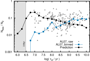
In our models, the ratio $N_{\mathrm{bss}}/N_{2}$ decreases in older populations. Binary evolution is more efficient in producing blue stragglers in high mass, young binaries than in low mass, old binaries. This is because the number of binaries that produce blue straggler stars by MS mergers and by stable mass transfer, i.e. the number of binaries that do not go through a common envelope phase, is larger in high mass than in low mass binaries (cf. Figs. 4 and 17–22). The peak in the predicted ratio $N_{\mathrm{bss}}/N_{2}$ around $10\,\mathrm{Myr}$ ($\log\tau_{\mathrm{cl}}/\mathrm{yr}=7$) is due to a change in the distribution functions of the initial orbital periods from Öpik’s law to the results of Sana et al. (2012) for O-star binaries (Sec. 2.2). The orbital period distribution of Sana et al. (2012) favours tight over wide binaries more than Öpik’s law does and thus binaries that form massive blue straggler stars.

A similar decreasing blue straggler ratio $N_{\mathrm{bss}}/N_{2}$ in older clusters is predicted from binary evolution calculations by Chen & Han (2009) but our ratios are larger by factors of $3$–$5$. Chen & Han (2009) notice a similar difference (of a factor of at most two) between their predicted blue straggler frequencies and those computed with the population synthesis code of Hurley et al. (2002). Chen & Han (2009) find that the difference is related to how they treat binaries in counting the number of stars two magnitudes below the turn-off. We count each binary as one stellar system because binaries are unresolved in the colour–magnitude diagrams from which the observed blue straggler frequencies are deduced. We notice another difference that might explain the discrepancy: we use a maximum initial orbital separation of $10^{4}\,{\rm R}_{\odot}$ while Chen & Han (2009) use $5.75\times 10^{6}\,{\rm R}_{\odot}$. Hence, our models contain more interacting binaries (cf. Fig. 4) that can form blue straggler stars. In other words, our effective binary fraction is larger.

The observations indicate an opposite trend to our models: the ratio $N_{\mathrm{bss}}/N_{2}$ increases with cluster age. There are complications that render a direct comparison between the observed and our predicted ratio $N_{\mathrm{bss}}/N_{2}$ difficult. There exist two classes of star clusters in the catalogue of Ahumada & Lapasset (2007): clusters with and without blue straggler stars. The bi-modality is mainly found in clusters younger than about $500\,\mathrm{Myr}$. There is no blue straggler star in $3\%$ of their star clusters older than $500\,\mathrm{Myr}$, in $38\%$ of star clusters with ages between $100$ and $500\,\mathrm{Myr}$ and in $80\%$ of star clusters younger than $100\,\mathrm{Myr}$. This bi-modality is not understood but causes the observed decreasing blue straggler frequency with younger cluster ages.

Stochastic sampling (Schneider et al. 2014b and Appendix D), i.e. lower number statistics in young clusters compared to older clusters because of the IMF, cannot explain this bi-modality. Stochastic sampling is expected to increase the scatter between the blue straggler frequencies of clusters of similar ages but not to create a bi-modal distribution. However, stochastic sampling may possibly complicate the accurate determination of the turn-off.

Supernova kicks (e.g. Lai 2001) might be part of the solution to this discrepancy. The binary companion of a blue straggler star that formed by RLOF, i.e. the former mass donor, will explode if it is massive enough to undergo core collapse. The supernova can break up the binary such that the blue straggler leaves the cluster as a runaway star, thereby reducing the number of blue stragglers observed in the cluster. Some clusters might lose all their blue stragglers in this way, giving rise to the observed bi-modality. The observed bi-modality is found in star clusters younger than $500\,\mathrm{Myr}$. However, supernova explosions occur only in young star clusters ($\lesssim 40\text{--}50\,\mathrm{Myr}$) with massive stars ($\gtrsim 7\text{--}8\,{\rm M}_{\odot}$). Supernova kicks can therefore explain only part of the discrepancy.

The primordial binary fraction in our models is $100\%$. A smaller binary fraction linearly decreases the number of blue stragglers and hence the ratio $N_{\mathrm{bss}}/N_{2}$. Our predictions are therefore likely upper limits, implying that our models underpredict the observed blue straggler frequencies in $\gtrsim 100\,\mathrm{Myr}$ star clusters and that additional channels for the formation of blue stragglers are required. Geller & Mathieu (2011) find carbon-oxygen white dwarfs as companions to blue stragglers in NGC 188. The white dwarf mass and period distributions appear to be consistent with a Case C RLOF formation scenario in which an asymptotic giant branch (AGB) star transfers mass to a MS star. In our models, RLOF from giants typically leads to common envelope evolution and thus not to the formation of blue stragglers. However, Chen & Han (2008) show that Case B and C mass transfer from giants to MS stars can form blue stragglers. Dynamical cluster evolution also produces blue stragglers in stellar collisions (e.g. Geller et al. 2013) and is expected to be more efficient the higher the density of the star cluster (e.g. Chatterjee et al. 2013). Another form of mass transfer, wind RLOF from AGB stars, might be efficient enough to also form blue straggler stars (e.g. Mohamed & Podsiadlowski 2007; Abate et al. 2013). All three contributions, the Case B and C formation scenarios, mergers due to collisions and wind RLOF, are missing in our predictions and might potentially help explaining the too low BSS predictions in $\gtrsim 100\,\mathrm{Myr}$ star clusters (see also Geller et al. 2013).

4.2. Binary fraction of blue straggler stars

A further testable prediction from our models is the binary fraction among blue straggler stars. The blue stragglers that form from stable mass transfer by RLOF can potentially be observed as binary stars whereas those that form from stellar mergers are observed as single stars. It is, however, difficult to observationally find the companions of blue stragglers that formed by stable mass transfer because the companions can be much fainter than the blue straggler (or even be a compact object) and the binary orbits are often wide such that most searches for radial velocity variations in blue stragglers cannot detect them (e.g. Collier & Jenkins 1984; Pols & Marinus 1994). The blue straggler binary might even be disrupted if the companion star explodes. In general, post-interaction binaries can often not be identified as such from radial velocity variations and mostly appear to be single stars (de Mink et al. 2014).

In our models, the binary fraction of blue straggler stars is independent of the primordial binary fraction in star clusters because only the sub-sample of primordial binaries can produce blue stragglers. The binary fraction among blue straggler stars is thus purely determined through binary evolution.

In Fig. 15 we show the binary fraction $f_{\mathrm{B}}$ of blue straggler and hence tail stars in our PDMFs as a function of cluster age. In our simulations we assume that all binaries with a mass ratio less than $0.56$ merge at the onset of RLOF during Case A mass transfer (Sec. 2.1), i.e. mass transfer from a MS star. Because of the assumed flat mass ratio distribution, at least $56\%$ of all Case A binaries merge and are thus observed as single stars ($f_{\mathrm{B}}\leq 44\%$). Our analysis of the binary parameter space (Figs. 17–22) reveals that more than $56\%$ of all binaries merge during Case A mass transfer because even binaries with a mass ratio greater than $0.56$ come into contact if they are initially in close orbits (e.g. Wellstein et al. 2001). In binaries younger than $2\,\mathrm{Myr}$, only the primary stars of very short orbit binaries overfill their Roche lobes. Most of them, regardless of the mass ratio, merge, leading to binary fractions $\leq 10\%$. Later, the binary fraction increases with time because also binaries in initially wider orbits interact, producing blue straggler stars by stable Case A and B mass transfer without merging, i.e. leaving behind a blue straggler in a binary.

Figure 15.— Binary fraction among blue straggler stars as a function of cluster age, $\tau_{\mathrm{cl}}$, corresponding to stars in the tail of our PDMFs. The given binary fractions are upper limits because we neglect supernova kicks that may disrupt binaries. The grey regions indicate ages for which boundary effects play a role.

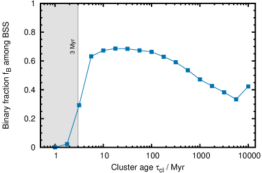
Case A mass transfer predominantly forms blue stragglers by merging in more than $56\%$ of all Case A binaries in our simulations. Contrarily, Case B mass transfer purely creates blue straggler star binaries (neglecting binary disruption by supernova explosions). The binary fraction in Fig. 15 therefore reaches a maximum of $\sim 60$–$70\%$ and stays at this level after all Case B binaries have enough time to interact to contribute blue straggler binaries.

In our models, Case B mass transfer in binaries with primary stars more massive than $5\,{\rm M}_{\odot}$ leads to fewer common envelope phases and consequently more blue stragglers than in binaries with less massive primary stars (cf. Case B regions of binaries with $2\,{\rm M}_{\odot}$ and $5\,{\rm M}_{\odot}$ primary stars in Figs. 17 and 18, respectively). The binary fraction of blue straggler stars therefore decreases in populations older than the lifetime of $5\,{\rm M}_{\odot}$ stars, i.e. older than $\sim 100\,\mathrm{Myr}$, and is given by the fraction of stars that merge during Case A (and early Case B) mass transfer.

Our blue straggler star binary fractions are upper limits because we neglect supernova kicks that might disrupt binaries and because the companions might be hard to detect observationally. We exclude supernova kicks because they introduce a random process that can only be fully taken into account by many repeated calculations which is impractical in our approach.

4.3. Apparent ages of blue straggler stars

Mass gainers and mergers appear to be younger than other cluster members because they are rejuvenated by mass accretion (Sec. 2.1). The age of a cluster is given by the MS lifetime of the turn-off stars, $\tau_{\mathrm{MS}}(M_{\mathrm{to}})\propto M_{\mathrm{to}}^{1-x}$, where $x$ is the exponent of the ML relation, $L\propto M^{x}$. The most massive blue straggler stars have a mass of about twice the mass of the turn-off stars in our models. Their apparent age is thus a factor $\tau_{\mathrm{MS}}(2M_{\mathrm{to}})/\tau_{\mathrm{MS}}(M_{\mathrm{to}})=2^{1-x}$ smaller than their true age if we neglect mixing of fresh fuel into convective cores which makes stars look even younger than the analytic approximation given here. The ML relation of MS stars is flatter, i.e. has a smaller exponent $x$, at high masses. The exponent approaches $x=1$ in stars close to the Eddington limit and is as large as $x=4$–$5$ in low mass stars ($\sim 1$–$2\,{\rm M}_{\odot}$). The most massive blue straggler with exponent $x=4$, i.e. a blue straggler of lower mass in older clusters, appears to be rejuvenated by a factor $1/8$ (the cluster appears eight times as old as the blue straggler). Contrarily, the most massive blue straggler with an exponent $x=2$, i.e. a blue straggler of higher mass in younger clusters, appears to be rejuvenated by only a factor of $1/2$ (the cluster appears twice as old as the blue straggler).

In Fig. 16 we show the apparent stellar age, $\tau_{*}$, of the most massive and of the apparently youngest blue straggler star in our simulations as a function of cluster age, $\tau_{\mathrm{cl}}$. The above mentioned trend for the most massive blue straggler is recovered, i.e. the most massive blue straggler in young star clusters appears to be less rejuvenated than in old ones: in a $10\,\mathrm{Myr}$ star cluster, the most massive blue straggler appears to be younger than the cluster by a factor of $0.48$ while this factor is smaller, only $0.17$, at $1\,\mathrm{Gyr}$.

Figure 16.— Apparent stellar age, $\tau_{*}$, of the most massive and the apparently youngest blue straggler star as a function of cluster age, $\tau_{\mathrm{cl}}$. The grey regions indicate ages for which boundary effects play a role.

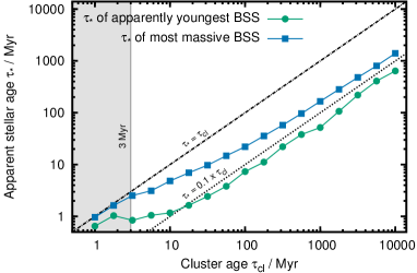
The most massive blue straggler is not the one that appears youngest (Fig. 16). The apparently youngest blue straggler forms from accretion onto a relatively unevolved star which then becomes a blue straggler. In our models, the apparently youngest blue straggler is about $40\%$ more massive than the turn-off and forms from late Case A/early Case B mass transfer in a binary with a mass ratio $0.5$–$0.6$. The mass ratio ensures that the secondary star is relatively unevolved. Mass accretion then brings the secondary mass above the mass of the turn-off, forming a blue straggler close to the ZAMS, i.e. apparently very young — the apparent age is of the order of $7\%$ of the cluster age (cf. Fig. 16).

The apparent age of the most massive blue straggler depends on how massive blue stragglers can get through mergers and stable RLOF, and on how much fresh fuel is mixed into convective cores during these processes. The apparent age of the most massive blue straggler is younger the more massive the star gets and the more mixing occurs. The apparent age of the seemingly youngest blue straggler depends on the choice of the critical mass ratios, $q_{\mathrm{crit}}$, and the mass transfer efficiency because these parameters determine how small the initial mass ratio can be in order to accrete enough mass to form a blue straggler star. The smaller the mass ratio, the less evolved is the progenitor of the blue straggler and hence the younger the blue straggler appears. Note that the mass ratio can also not be too small: there has to be enough transferred mass such that the secondary mass can exceed the turn-off mass.

5. Determination of star cluster ages

As shown in Sec. 4.3, a stellar population can be 10 times older than some of its most massive stars appear to be. Such rejuvenated stars can bias the age determination of stellar populations because it is not always clear whether a star was influenced by binary mass transfer in the past or not. Especially in young clusters with OB stars, the most luminous and hence most massive stars are often investigated in detail because they are easiest to observe. Their ages are then sometimes interpreted as the cluster age although the most massive stars are likely rejuvenated binary products.

To avoid potential biases and confusion of stars with rejuvenated binary products such as stellar mergers, stars at least half the mass of the most massive cluster members should be used to determine ages of stellar populations. This rule of thumb is implicitly taken into account when dismissing blue stragglers from fitting the turn-off of well-populated star clusters in colour–magnitude or HR diagrams.

The turn-off may be blurred by binary products and it is sometimes, especially in young star clusters, challenging to determine its location. In such cases, the mass function may provide a promising alternative because possibly rejuvenated binary products can be identified by the binary tail and the age of the stellar population can be directly determined by reading-off the turn-off mass.

First, we consider single star mass functions to clarify the general approach to determine cluster ages from mass functions. Single star mass functions are truncated at the present-day turn off mass, $M_{{\rm to,p}}$, because of finite stellar lifetimes. The present-day and initial mass of the turn off stars in old stellar populations are the same because stars have negligible stellar winds. The age of old populations therefore follows directly from the MS age of stars with an initial mass of that of the turn-off. In young stellar populations, stars lose mass by stellar winds and a peak forms in the mass function. The present-day mass of the turn off stars that is read-off from the truncation of the mass function is no longer equal to their initial mass because of stellar winds. However, without further modeling or the need of stellar models, we can correct for wind mass loss by redistributing the number of excess stars in the wind mass loss peak, $N_{1}$, such that the mass function is filled up to the initial mass of the turn off stars, $M_{{\rm to,i}}$ (cf. Fig. 6 and Sec. 3.1). Rewriting the mass lost by stellar winds on the MS, $\Delta M=M_{\mathrm{to,i}}-M_{\mathrm{to,p}}$, in Eq. (10), we have for the number of excess stars in the wind mass loss peak,

$$N_{1}=\frac{A}{\Gamma}\left(M_{{\rm to,i}}^{\Gamma}-M_{{\rm to,p}}^{\Gamma}\right)\,,$$ (17)

from which we find the initial mass of the turn-off stars,

$$M_{{\rm to,i}}=\left(\frac{N_{1}\Gamma}{A}+M_{{\rm to,p}}^{\Gamma}\right)^{1/\Gamma},$$ (18)

in the cluster. The age of the star cluster follows from the MS lifetime of the turn off stars with initial mass $M_{{\rm to,i}}$.

The mass function of binary stars allows us to determine the age of the stellar population in a similar way. The difference is that the binary star mass functions are not truncated at the turn-off mass but rather at about twice this mass. In practice the mass function may be truncated at less than twice the turn-off mass because of stochastic sampling. Consequently, another indicator of the turn-off mass than the truncation of the mass function is required to determine the age of the stellar population. We use the onset of the binary tail for that purpose. In old stellar populations, the onset of the binary tail, i.e. the turn-off mass, is indicated by a steep decrease in the number of stars. In young stellar populations, the number of stars in our models do not change that strongly at the onset of the binary tail. In such cases, we propose the use of the wind mass loss peak to indicate the onset of the binary tail and hence to determine the turn-off mass and the age of the stellar population. The number of excess stars in the peak can be influenced by unresolved binaries and binary evolution (Sec. 3.2). The correction for stellar wind mass loss to derive the initial mass of the turn off stars may therefore not be possible without the use of stellar models that provide the mapping of masses at the end of the MS to initial masses.

The advantage of this over other methods to determine stellar ages is that it is not biased by apparently younger, rejuvenated binary products. Instead, the proposed method identifies and explicitly uses rejuvenated binary products to determine the turn-off mass and hence to derive the cluster age.

This new method is used by Schneider et al. (2014b) to determine the ages of the young Arches and Quintuplet star clusters in the Galactic centre. The mass functions of Arches and Quintuplet show a wind mass loss peak from which it is possible to identify the binary tail and derive an unambiguous age. The age from the wind mass loss peak results in older cluster ages than previously derived for these clusters from the most luminous stars. The most luminous stars belong to the binary tail of the mass function and are thus likely rejuvenated binary products.

6. Conclusions

We use a rapid binary evolution code to investigate how single and binary star evolution shape PDMFs with time. To that end, we set up coeval populations of single and binary stars, follow their evolution in time and construct mass functions at ages ranging from $\mathrm{Myr}$ up to $\mathrm{Gyr}$. Our code incorporates all the relevant single and binary star physics that directly alters stellar masses — wind mass loss, mass transfer in binaries by RLOF and by winds, stellar mergers and rejuvenation of stars.

Finite stellar lifetimes truncate the mass functions and wind mass loss results in an accumulation of stars in the PDMF creating a peak at the high mass end. The magnitude of the peak depends on the strength of stellar winds, i.e. on stellar mass and metallicity, and the slope of the IMF: the flatter the IMF the stronger the peak. The peak can thus be used to constrain stellar wind mass loss. We investigate the age and mass ranges of stellar populations for which we expect a wind mass loss peak in their mass functions. Typically, the peak is present in stellar populations younger than about $10\,\mathrm{Myr}$ at $Z=0.02$ corresponding to stars initially more massive than about $18\,{\rm M}_{\odot}$ (Figs. 6 and 7). Less massive stars have too weak stellar winds. The peak flattens the PDMF slopes at the high mass end by up to $60\%$ in $5\,\mathrm{Myr}$ old stellar populations with a Salpeter IMF (IMF slope $\Gamma=-1.35$; Fig. 11).

Binary interaction, i.e. mass transfer and stellar mergers, reshape the PDMF at the high mass end, forming a tail which extends the PDMF of single stars by a factor of 2 in mass. The PDMF tail consists of rejuvenated binary products that are not expected to exist from single star evolution and are better known as blue stragglers. Binary interactions are more efficient in producing the binary tail at high masses (Sec. 2.3). The number of rejuvenated binary products in young star clusters ($\sim 5\,{\rm Myr}$) reaches more than $30\%$ of the initial number of stars in the mass range corresponding to the tail (Figs. 12 and 13). Binary interactions are therefore efficient in repopulating the high mass end of PDMFs even in star clusters that are only a couple of million years old.

Unresolved binaries flatten the slope of the PDMF. The slope is flattened by about $0.1$ in our zero-age populations, which is in agreement with previous work on unresolved multiple systems. Altogether, stellar winds, mass exchange in binary systems and unresolved binaries reshape the high mass end of mass functions within $\pm 0.3\,\mathrm{dex}$ of the turn-off mass and can therefore bias IMF determinations.

We compare our predicted blue straggler frequencies to those from the blue straggler catalogue of Galactic open star clusters (Ahumada & Lapasset 2007). Our models predict a decreasing blue straggler frequencies with increasing cluster age — in contrast to the observations. The observed blue straggler frequency drops with younger ages because there are no blue stragglers identified in two-thirds of the open clusters younger than $500\,\mathrm{Myr}$ but only in $3\%$ of clusters older than that. Our models predict about the right amount of blue stragglers in young clusters ($\lesssim 100\,\mathrm{Myr}$) but too few in older clusters. Additional blue straggler formation channels, such as mergers resulting from stellar collisions and wind Roche-lobe overflow from AGB stars, are likely required to explain the observed frequency of blue stragglers in older clusters. Also, the treatment of Case B and C mass transfer may need revision in our models to allow for the formation of blue stragglers from RLOF of giants to MS stars.

The binary fraction among the blue straggler stars in the tail of our PDMFs varies between $40\%$ and $70\%$, depending on cluster age. It is largest in young ($\sim 10\,\mathrm{Myr}$) and smallest in old stellar populations ($\sim 5000\,\mathrm{Myr}$). Our binary fractions are upper limits because we neglect supernova kicks that may disrupt binaries.

The most massive blue stragglers in the binary tail have apparent ages that are younger by factors of $0.17$–$0.48$ than the real cluster age, i.e. cluster ages inferred from the most massive stars would be too young by factors of $2$–$6$. Some of the less massive blue stragglers may show apparent ages that are even younger by a factor of 10. Cluster ages derived from the most luminous stars should therefore be treated with caution because of a likely confusion with rejuvenated binary products. If in doubt, and to avoid potential confusion, cluster ages should not be based on the most luminous cluster members. Instead, we propose the use of mass functions to identify rejuvenated binary products and to derive cluster ages. This is possible because the turn-off mass and hence the cluster age can be directly determined from mass functions.

In old stellar populations, the turn-off mass is best indicated by a steep decrease of the number of stars at the onset of the binary tail. In younger populations, this decrease of the number of stars is less and the wind mass loss peak may be used instead to determine the turn-off mass. Stellar mass functions and especially the wind mass loss peak constitute a new and unambiguous clock to age-date star clusters. This technique is applied by Schneider et al. (2014b) to the Arches and Quintuplet star clusters to determine unambiguous cluster ages by identifying likely binary products and thereby resolved the apparent age discrepancies among the most luminous members in both clusters.

The binary products in the tail of young PDMFs have potentially far-reaching consequences. So far, they have mostly been neglected when computing the feedback from stellar populations. However, the stars in the tail are the most massive stars in a stellar population and can therefore contribute significantly to the ionising radiation, the mechanical feedback from stellar winds and supernovae explosions and to the chemical enrichment. In the youngest star clusters, binary products might even become so massive that they explode as pair-instability supernovae, thereby contributing significantly to the metal production in the Universe (Heger & Woosley 2002; Gal-Yam et al. 2009; Langer 2012).

Appendix A Binary parameter space continued

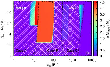
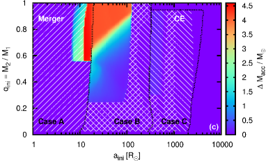
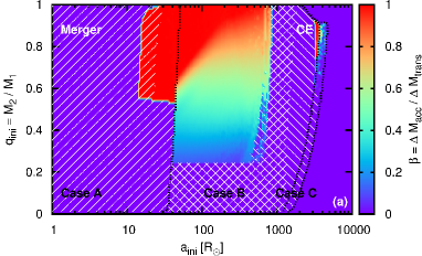
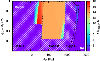
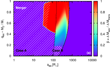
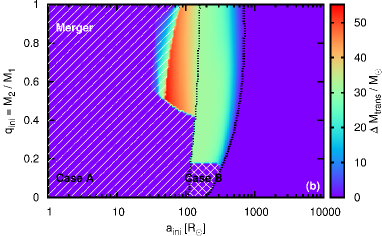
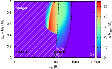
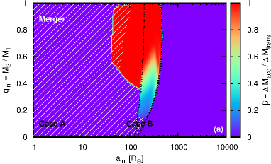
In Sec. 2.3 we describe how much mass is transferred and accreted in our binary models with $10\,{\rm M}_{\odot}$ primary stars to understand quantitatively how binary evolution shapes the high mass end of PDMFs. Here, we continue this description by providing figures equivalent to Figs. 1, 2 and 3 but for primary masses of $2$, $5$, $20$, $50$, $70$ and $100\,{\rm M}_{\odot}$ (Figs. 18–22, respectively). These analyses enable us to fully understand the quantitative results presented in this paper. The top panels (a) contain the mass transfer efficiency $\beta$ as defined in Eq. (8), the middle panels (b) the mass transferred from the primary to the secondary stars during stable RLOF and the bottom panels (c) the mass accreted by the secondary stars during stable RLOF.

$\mathbf{M_{1}=2\,{\rm M}_{\odot}}$

Figure 17.— Mass transfer efficiency $\beta$ (top panel (a)), transferred mass from primary to secondary during stable RLOF (middle panel (b)) and mass accreted by secondary star during stable RLOF (bottom panel (c)) as functions of the initial mass ratio $q_{\mathrm{ini}}$ (i.e. initial secondary mass) and initial orbital separation $a_{\mathrm{ini}}$ for $2\,{\rm M}_{\odot}$ primary stars. The shaded regions have the same meaning as in Fig. 1 and indicate binaries which merge and/or go through a common envelope phase.

$\mathbf{M_{1}=5\,{\rm M}_{\odot}}$

Figure 18.— As Fig. 17 but for $5\,{\rm M}_{\odot}$ primary stars.

$\mathbf{M_{1}=20\,{\rm M}_{\odot}}$

Figure 19.— As Fig. 17 but for $20\,{\rm M}_{\odot}$ primary stars.

$\mathbf{M_{1}=50\,{\rm M}_{\odot}}$

Figure 20.— As Fig. 17 but for $50\,{\rm M}_{\odot}$ primary stars.

$\mathbf{M_{1}=70\,{\rm M}_{\odot}}$

Figure 21.— As Fig. 17 but for $70\,{\rm M}_{\odot}$ primary stars.

$\mathbf{M_{1}=100\,{\rm M}_{\odot}}$

Figure 22.— As Fig. 17 but for $100\,{\rm M}_{\odot}$ primary stars.

Appendix B Uncertainties in the models

B.1. Single star evolution

Stars more massive than $10\,{\rm M}_{\odot}$ accumulate in a peak at the high mass end of PDMFs because of stellar wind mass loss (Sec. 3.1). The magnitude of the accumulation depends on the IMF slope $\Gamma$ and on the strength of stellar winds, i.e. on the wind mass loss prescription and the metallicity. Our wind mass loss prescription for MS stars (Nieuwenhuijzen & de Jager 1990; Kudritzki et al. 1989) tends to slightly underestimate stellar wind mass loss compared to Vink et al. (2000, 2001). We compare our initial and end-of-MS stellar masses to the latest non-rotating stellar models of Brott et al. (2011) and Ekström et al. (2012) and find that the turn-off masses agree within $1$–$3\%$ for stars less massive than about $50\,{\rm M}_{\odot}$ and that we overestimate the turn-off masses by up to $20\%$ for more massive stars. This deviation is primarily because of the Wolf–Rayet wind mass loss rates used in Brott et al. (2011) and Ekström et al. (2012) for massive MS stars which we only apply for post-MS stars. Increasing the wind mass loss for stars $\geq 50\,{\rm M}_{\odot}$ to match the turn-off masses of the latest detailed stellar models results into stronger peaks at the high mass end of PDMF younger than about $4.3\,\mathrm{Myr}$. Older populations are not affected.

The wind mass loss peak flattens PDMFs (Sec. 3.4). Whether this effect needs to be taken into account when deriving the IMF from observations depends on how mass functions are constructed from a measured sample of stars. If, on the one hand, measured stellar luminosities are converted to masses by means of a suitable ML relation, the flattening of the PDMF by wind mass loss needs to be taken into account. If, on the other hand, the observed stars are compared individually to stellar evolution tracks to find their initial masses, this effect does not need to be corrected for because stellar tracks usually include wind mass loss. Alternatively, the mass function slope can be determined omitting the high mass end and therefore the wind mass loss peak.

B.2. Uncertain binary physics

In this section we discuss changes in the treatment of binary interactions and their importance for the PDMFs. Besides mass, angular momentum is transferred during RLOF. Packet (1981) found that a uniformly rotating star needs to accrete only 5–10% of its initial mass through a disc to reach a critical (Keplerian) velocity at the equator such that the outermost layers are no longer bound to the star (see also Petrovic et al. 2005). This point of view is debated and there are several arguments regarding accretion and decretion disks which might be able to dissipate angular momentum such that stars stay always below critical rotation and thus can accrete much more mass (Lin & Pringle 1976; Popham & Narayan 1991; Krtička et al. 2011). If a star is spun up to over-critical rotation it probably sheds as much mass as is needed to rotate below critical. Mass is lost from the system and takes away angular momentum from the star. In the case of RLOF this means that not all transferred mass is accreted, mass transfer is non-conservative and typically only a few percent of the transferred mass is accreted (Langer 2012). Low mass transfer efficiencies reduce the PDMF binary tail. For stellar mergers we assume that $10\%$ of the system mass is lost and takes away the excess angular momentum. This is likely rather an upper limit because detailed collision simulations of massive MS stars show that $<10\%$ is lost even in equal-mass merger events (Glebbeek et al. 2013).

Detailed binary models find mass transfer efficiencies of about $100\%$ for Case A and of the order of $40$–$100\%$ for early Case B mass transfer (Wellstein et al. 2001). Also, tides in short period binaries and magnetic fields in combination with mass loss (e.g., by a stellar wind), i.e. magnetic braking, are efficient in dissipating angular momentum such that stars do not reach critical rotation during RLOF. Magnetic fields seem to be even generated by strong shear because of mass accretion (see e.g., Plaskett’s star, Grunhut et al. 2013) and stellar mergers (Tout et al. 2008; Ferrario et al. 2009; Langer 2012).

It is mentioned by Hurley et al. (2002) that the critical mass ratio $q_{{\rm crit}}=m_{2}/m_{1}=0.25$ that determines whether stars come into contact during thermal timescale mass transfer, e.g., when the primary star is a Hertzsprung gap star, is rather approximate. Case B mass transfer can lead to a contact phase for extreme mass ratios because the mass transfer timescale becomes faster than the thermal timescale of the accretor (e.g. Ulrich & Burger 1976; Kippenhahn & Meyer-Hofmeister 1977; Neo et al. 1977; Pols & Marinus 1994; Wellstein et al. 2001). We implement a similar criterion with the consequence that nearly all binary systems undergoing Case B mass transfer go through a contact phase in which both stars merge or eject their common envelopes. Merging stars results in a post-MS object and hence a reduction of MS secondary stars. Ejecting envelopes terminates any mass transfer such that the initial secondary stars cannot accrete any matter — in other words the mass transfer efficiency is $0\%$ for most Case B binaries. The resulting changes to our PDMFs are small, because we already limit mass accretion to the thermal timescale of the accretors.

The initial distribution functions of secondary masses (or mass ratios) and orbital periods are also important for our results. We assume an initially flat mass ratio distribution, i.e. all mass ratios are equally probable. Small initial mass ratios often lead to contact phases (see the discussion of the binary parameter space in Sec. 2.3). A distribution function of initial mass ratios which favours equal mass binaries enhances the effect of mass transfer and reduces the effect of MS coalescence. Also the Case B contribution, which is the dominant mass transfer channel at later times (Fig. 9), is increased because the Case B mass transfer efficiency is higher for larger mass ratios. If the initial orbital separation distribution favours small initial orbital separations compared to Öpik’s law, Case A and B mass transfer (including stellar mergers) occur more frequently which increases the magnitude of the tail of the PDMFs.

Different IMF slopes $\Gamma$ enhance or reduce the importance of binary physics. Binary evolution usually increases the mass of stars: let this increase be given by a multiplicative factor $\alpha$, i.e. the increased mass is $\alpha M$. If we increase all stellar masses $M$ by the same factor $\alpha$, we enhance the mass function at the increased mass $\alpha M$ by the factor,

$$\frac{\psi(\ln M)}{\psi(\ln\alpha M)}=\alpha^{-\Gamma}.$$ (B1)

The steeper the slope of the IMF, i.e. the more negative $\Gamma$, the bigger the effect of any mass gain. Also the flattening of the PDMF because of unresolved binaries is more important for steeper IMF slopes and less important for flatter IMF slopes (Sec. 3.4). This trend is opposite if mass is lost e.g., by stellar winds: then, a flatter IMF enhances and a steeper one reduces the accumulation of stars.

Appendix C Unresolved binary stars

Binaries in photometric studies are usually unresolved which leads to an overestimation of their masses (see Eq. 15). A mass function, even at zero age, thus looks different compared to the IMF. We find changes in the slope of the mass function of the order of $\Delta\beta\approx 0.1$ toward flattened mass functions for zero age populations. The flattening because of unresolved binaries is more important for larger masses because of the mass dependence of the power law index of the ML relation (Sec. 3.4). The problem of unresolved binaries is well known (Sagar & Richtler 1991; Kroupa et al. 1993; Maíz Apellániz 2008; Weidner et al. 2009). To compare with their results it is important to know how they distributed stars in binaries (see e.g., the review by Bastian et al. 2010).

Sagar & Richtler (1991), for example, do not use a flat mass ratio distribution, but they draw both binary components randomly from one IMF. For an initial IMF slope of $\Gamma=-1.5$ (our initial IMF slope is Salpeter, i.e. $\Gamma=-1.35$) and a binary fraction of 50% they derive a PDMF slope of $\beta=-1.16$; for a binary fraction of 100% they arrive at $\beta=-1.10$. These changes occur according to their analysis in a mass range of $2$–$14\,{\rm M}_{\odot}$ and are larger than we find. The major difference between their calculation and ours is the assumed distribution function of stars in binaries (mass ratios and IMF slope).

Maíz Apellániz (2008) not only investigates unresolved binary stars but also higher order multiples and chance superpositions in dense clusters. Taking only the effect of binary stars into account they conclude “that for most cases the existence of unresolved binaries has only a small effect on the massive-star IMF slope” of the order of $|\Delta\beta|\approx 0.2$. They use the same mass ratio distribution as in our analysis but slightly different IMF slopes.

Weidner et al. (2009) investigate the effect of unresolved binaries and higher order multiples for different pairing methods. None of their pairing methods correspond to our flat mass ratio distribution. A steepening of the observed PDMF by $\Delta\beta=0.1$ is reported. Their PDMF is steeper because they take a certain number of stars given by their IMF and pair them randomly into binaries (their RP method). The probability of finding a massive star grouped with another massive star is therefore less than to find it grouped with a lower mass companion, hence estimated system masses do not change significantly for massive stars. At lower masses it is opposite: relatively more binaries with stars of similar masses are found and the companions lead to higher system mass estimates. In total this leads to a steepening of the PDMF.

All in all it seems that unresolved binaries have limited influence on the PDMF of zero age populations. Pairing stars which are randomly sampled from an IMF steepens the mass function, whereas a flat mass ratio distribution flattens the mass function as is shown in our analysis. Observations of massive, i.e. O-type binaries favour a flat mass ratio distribution (Sana et al. 2012), so the high mass end of PDMFs of young stellar populations with O-type stars is expected to be flattened if binaries are unresolved.

Appendix D Stochastic sampling

The statement that the most massive stars are likely blue stragglers has to be treated with caution, because it is only valid in “rich” (i.e. massive) clusters where there are enough stars to sample the binary parameter space well — this problem is known as stochastic sampling. Binary evolution e.g., re-populates the $5\,\mathrm{Myr}$ PDMF on average by more than $40\%$ of the IMF above $40\,{\rm M}_{\odot}$ ($\log m\approx 1.6$). If there is initially only one star in this mass range, we expect about $0.4$ stars to be re-populated by binary evolution — if there are initially 10 stars (if the cluster is a factor of 10 more massive), we expect to find about four binary products. So if the cluster is not massive enough, there might be no blue straggler star at a certain age. It will also take some time until binary star evolution produces the first blue straggler stars. This again depends on the cluster richness and on how binaries are distributed: the shorter the initial period, the earlier the binary interaction. When the initially most massive stars in a cluster evolve toward the end of core hydrogen burning we know that blue stragglers can be produced by MS mergers and Case A mass transfer. So the whole contribution of MS mergers and Case A mass transfer products of binaries with initial $100\,{\rm M}_{\odot}$ primary stars to the blue straggler star population is expected to be present after about $3\,\mathrm{Myr}$. Blue stragglers can be even present at younger ages — this is just a matter of stochastic sampling which is investigated in more detail in Schneider et al. (2014b).

References

- Abate et al. (2013) Abate, C., Pols, O. R., Izzard, R. G., Mohamed, S. S., & de Mink, S. E. 2013, A&A, 552, A26
- Ahumada & Lapasset (2007) Ahumada, J. A., & Lapasset, E. 2007, A&A, 463, 789
- Barnes (2007) Barnes, S. A. 2007, ApJ, 669, 1167
- Bastian et al. (2010) Bastian, N., Covey, K. R., & Meyer, M. R. 2010, ARA&A, 48, 339
- Braun & Langer (1995) Braun, H., & Langer, N. 1995, A&A, 297, 483
- Brott et al. (2011) Brott, I., de Mink, S. E., Cantiello, M., et al. 2011, A&A, 530, A115
- Chatterjee et al. (2013) Chatterjee, S., Rasio, F. A., Sills, A., & Glebbeek, E. 2013, ApJ, 777, 106
- Chen & Han (2008) Chen, X., & Han, Z. 2008, MNRAS, 387, 1416
- Chen & Han (2009) —. 2009, MNRAS, 395, 1822
- Collier & Jenkins (1984) Collier, A. C., & Jenkins, C. R. 1984, MNRAS, 211, 391
- de Grijs et al. (2002) de Grijs, R., Gilmore, G. F., Johnson, R. A., & Mackey, A. D. 2002, MNRAS, 331, 245
- de Mink et al. (2013) de Mink, S. E., Langer, N., Izzard, R. G., Sana, H., & de Koter, A. 2013, ApJ, 764, 166
- de Mink et al. (2007) de Mink, S. E., Pols, O. R., & Hilditch, R. W. 2007, A&A, 467, 1181
- de Mink et al. (2014) de Mink, S. E., Sana, H., Langer, N., Izzard, R. G., & Schneider, F. R. N. 2014, ApJ, 782, 7
- Dray & Tout (2007) Dray, L. M., & Tout, C. A. 2007, MNRAS, 376, 61
- Duchêne & Kraus (2013) Duchêne, G., & Kraus, A. 2013, ARA&A, 51, 269
- Ekström et al. (2012) Ekström, S., Georgy, C., Eggenberger, P., et al. 2012, A&A, 537, A146
- Ferrario et al. (2009) Ferrario, L., Pringle, J. E., Tout, C. A., & Wickramasinghe, D. T. 2009, MNRAS, 400, L71
- Gal-Yam et al. (2009) Gal-Yam, A., Mazzali, P., Ofek, E. O., et al. 2009, Nature, 462, 624
- Geller et al. (2013) Geller, A. M., Hurley, J. R., & Mathieu, R. D. 2013, AJ, 145, 8
- Geller & Mathieu (2011) Geller, A. M., & Mathieu, R. D. 2011, Nature, 478, 356
- Glebbeek et al. (2013) Glebbeek, E., Gaburov, E., Portegies Zwart, S., & Pols, O. R. 2013, MNRAS, 434, 3497
- Glebbeek & Pols (2008) Glebbeek, E., & Pols, O. R. 2008, A&A, 488, 1017
- Grunhut et al. (2013) Grunhut, J. H., Wade, G. A., Leutenegger, M., et al. 2013, MNRAS, 428, 1686
- Habibi et al. (2013) Habibi, M., Stolte, A., Brandner, W., Hußmann, B., & Motohara, K. 2013, A&A, 556, A26
- Harfst et al. (2010) Harfst, S., Portegies Zwart, S., & Stolte, A. 2010, MNRAS, 409, 628
- Heger & Woosley (2002) Heger, A., & Woosley, S. E. 2002, ApJ, 567, 532
- Holmberg et al. (2007) Holmberg, J., Nordström, B., & Andersen, J. 2007, A&A, 475, 519
- Humphreys & Davidson (1979) Humphreys, R. M., & Davidson, K. 1979, ApJ, 232, 409
- Hurley et al. (2005) Hurley, J. R., Pols, O. R., Aarseth, S. J., & Tout, C. A. 2005, MNRAS, 363, 293
- Hurley et al. (2000) Hurley, J. R., Pols, O. R., & Tout, C. A. 2000, MNRAS, 315, 543
- Hurley et al. (2001) Hurley, J. R., Tout, C. A., Aarseth, S. J., & Pols, O. R. 2001, MNRAS, 323, 630
- Hurley et al. (2002) Hurley, J. R., Tout, C. A., & Pols, O. R. 2002, MNRAS, 329, 897
- Izzard et al. (2006) Izzard, R. G., Dray, L. M., Karakas, A. I., Lugaro, M., & Tout, C. A. 2006, A&A, 460, 565
- Izzard et al. (2009) Izzard, R. G., Glebbeek, E., Stancliffe, R. J., & Pols, O. R. 2009, A&A, 508, 1359
- Izzard et al. (2004) Izzard, R. G., Tout, C. A., Karakas, A. I., & Pols, O. R. 2004, MNRAS, 350, 407
- Kippenhahn & Meyer-Hofmeister (1977) Kippenhahn, R., & Meyer-Hofmeister, E. 1977, A&A, 54, 539
- Kippenhahn & Weigert (1967) Kippenhahn, R., & Weigert, A. 1967, ZAp, 65, 251
- Köhler et al. (2012) Köhler, K., Borzyszkowski, M., Brott, I., Langer, N., & de Koter, A. 2012, A&A, 544, A76
- Kroupa et al. (1993) Kroupa, P., Tout, C. A., & Gilmore, G. 1993, MNRAS, 262, 545
- Kroupa et al. (2013) Kroupa, P., Weidner, C., Pflamm-Altenburg, J., et al. 2013, The Stellar and Sub-Stellar Initial Mass Function of Simple and Composite Populations, ed. T. D. Oswalt & G. Gilmore, 115
- Krtička et al. (2011) Krtička, J., Owocki, S. P., & Meynet, G. 2011, A&A, 527, A84+
- Kudritzki et al. (1989) Kudritzki, R. P., Pauldrach, A., Puls, J., & Abbott, D. C. 1989, A&A, 219, 205
- Lai (2001) Lai, D. 2001, in Lecture Notes in Physics, Berlin Springer Verlag, Vol. 578, Physics of Neutron Star Interiors, ed. D. Blaschke, N. K. Glendenning, & A. Sedrakian, 424
- Langer (2012) Langer, N. 2012, ARA&A, 50, 107
- Lauterborn (1970) Lauterborn, D. 1970, A&A, 7, 150
- Leigh et al. (2011) Leigh, N., Sills, A., & Knigge, C. 2011, MNRAS, 415, 3771
- Levenberg (1944) Levenberg, K. 1944, Quart. Applied Math., 2, 164
- Lin & Pringle (1976) Lin, D. N. C., & Pringle, J. E. 1976, in IAU Symposium, Vol. 73, Structure and Evolution of Close Binary Systems, ed. P. Eggleton, S. Mitton, & J. Whelan, 237–+
- Lombardi et al. (1995) Lombardi, Jr., J. C., Rasio, F. A., & Shapiro, S. L. 1995, ApJ, 445, L117
- Maíz Apellániz (2008) Maíz Apellániz, J. 2008, ApJ, 677, 1278
- Marquardt (1963) Marquardt, D. W. 1963, SIAM Journal on Applied Mathematics, 11, 431
- McLaughlin & Fall (2008) McLaughlin, D. E., & Fall, S. M. 2008, ApJ, 679, 1272
- Mohamed & Podsiadlowski (2007) Mohamed, S., & Podsiadlowski, P. 2007, in Astronomical Society of the Pacific Conference Series, Vol. 372, 15th European Workshop on White Dwarfs, ed. R. Napiwotzki & M. R. Burleigh, 397
- Monteiro et al. (2010) Monteiro, H., Dias, W. S., & Caetano, T. C. 2010, A&A, 516, A2
- Naylor & Jeffries (2006) Naylor, T., & Jeffries, R. D. 2006, MNRAS, 373, 1251
- Neo et al. (1977) Neo, S., Miyaji, S., Nomoto, K., & Sugimoto, D. 1977, PASJ, 29, 249
- Nieuwenhuijzen & de Jager (1990) Nieuwenhuijzen, H., & de Jager, C. 1990, A&A, 231, 134
- Öpik (1924) Öpik, E. 1924, Publications of the Tartu Astrofizica Observatory, 25, 1
- Packet (1981) Packet, W. 1981, A&A, 102, 17
- Petrovic et al. (2005) Petrovic, J., Langer, N., & van der Hucht, K. A. 2005, A&A, 435, 1013
- Pols & Marinus (1994) Pols, O. R., & Marinus, M. 1994, A&A, 288, 475
- Pols et al. (1998) Pols, O. R., Schroder, K.-P., Hurley, J. R., Tout, C. A., & Eggleton, P. P. 1998, MNRAS, 298, 525
- Popham & Narayan (1991) Popham, R., & Narayan, R. 1991, ApJ, 370, 604
- Sagar & Richtler (1991) Sagar, R., & Richtler, T. 1991, A&A, 250, 324
- Salpeter (1955) Salpeter, E. E. 1955, ApJ, 121, 161
- Sana et al. (2012) Sana, H., de Mink, S. E., de Koter, A., et al. 2012, Science, 337, 444
- Scalo (1986) Scalo, J. M. 1986, Fund. Cosmic Phys., 11, 1
- Schneider et al. (2014a) Schneider, F. R. N., Langer, N., de Koter, A., et al. 2014a, A&A, 570, A66
- Schneider et al. (2014b) Schneider, F. R. N., Izzard, R. G., de Mink, S. E., et al. 2014b, ApJ, 780, 117
- Sills et al. (2001) Sills, A., Faber, J. A., Lombardi, Jr., J. C., Rasio, F. A., & Warren, A. R. 2001, ApJ, 548, 323
- Sills et al. (2013) Sills, A., Glebbeek, E., Chatterjee, S., & Rasio, F. A. 2013, ApJ, 777, 105
- Sills et al. (1997) Sills, A., Lombardi, Jr., J. C., Bailyn, C. D., et al. 1997, ApJ, 487, 290
- Soderblom (2010) Soderblom, D. R. 2010, ARA&A, 48, 581
- Tout et al. (1997) Tout, C. A., Aarseth, S. J., Pols, O. R., & Eggleton, P. P. 1997, MNRAS, 291, 732
- Tout et al. (1996) Tout, C. A., Pols, O. R., Eggleton, P. P., & Han, Z. 1996, MNRAS, 281, 257
- Tout et al. (2008) Tout, C. A., Wickramasinghe, D. T., Liebert, J., Ferrario, L., & Pringle, J. E. 2008, MNRAS, 387, 897
- Ulrich & Burger (1976) Ulrich, R. K., & Burger, H. L. 1976, ApJ, 206, 509
- van Bever & Vanbeveren (1998) van Bever, J., & Vanbeveren, D. 1998, A&A, 334, 21
- Vanbeveren (1991) Vanbeveren, D. 1991, A&A, 252, 159
- Vink et al. (2000) Vink, J. S., de Koter, A., & Lamers, H. J. G. L. M. 2000, A&A, 362, 295
- Vink et al. (2001) —. 2001, A&A, 369, 574
- Weidner et al. (2009) Weidner, C., Kroupa, P., & Maschberger, T. 2009, MNRAS, 393, 663
- Wellstein et al. (2001) Wellstein, S., Langer, N., & Braun, H. 2001, A&A, 369, 939