Long signal change-point detection

Abstract

The detection of change-points in a spatially or time-ordered data sequence is an important problem in many fields such as genetics and finance. We derive the asymptotic distribution of a statistic recently suggested for detecting change-points. Simulation of its estimated limit distribution leads to a new and computationally efficient change-point detection algorithm, which can be used on very long signals. We assess the algorithm experimentally under various conditions.

I.   Introduction

When met with a data set ordered by time or space, it is often important to predict when or where something “changed” as we move temporally or spatially through it. In biology, for example, changes in an array Comparative Genomic Hybridization (aCGH) or Chip-Seq data signal as one moves across the genome can represent an event such as a change in genomic copy number, which is extremely important in cancer gene detection [17, 22]. In the financial world, detecting changes in multivariate time-series data is important for decision-making [27]. Change-point detection can also be used to detect financial anomalies [3] and significant changes in a sequence of images [11].

Change-point detection analysis is a well-studied field and there are numerous approaches to the problem. Its extensive literature ranges from parametric methods using log-likelihood functions [4, 14] to nonparametric ones based on Wilcoxon-type statistics, U-statistics and sequential ranks. The reader is referred to the monograph [5] for an in-depth treatment of these methods.

In change-point modeling it is generally supposed that we are dealing with a random process evolving in time or space. The aim is to develop a method to search for a point where possible changes occur in the mean, variance, distribution, etc. of the process. All in all, this comes down to finding ways to decide whether a given signal can be considered homogeneous in a statistical (stochastic) sense.

The present article builds upon an interesting nonparametric change-point detection method that was recently proposed by Matteson and James [15]. It uses U-statistics (see [9]) as the basis of its change-point test. Its interest lies in its ability to detect quite general types of change in distribution. Several theoretical results are presented in [15] to highlight some of the mathematical foundations of their method. These in turn lead to a simple and useful data-driven statistical test for change-point detection. The authors then apply this test successfully to simulated and real-world data.

There are however several weaknesses in [15] both from theoretical and practical points of view. Certain fundamental theoretical considerations are incompletely treated, especially the assertion that a limit distribution exists for the important statistic, upon which the rest of the approach hangs. On the practical side, the method is computationally prohibitive for signals of more than a few thousand points, which is unfortunate because real-world signals can be typically much longer.

Our paper has two main objectives. First, it fills in missing theoretical results in [15] including a derivation of the limit distribution of the statistic. This requires the effective application of large sample theory techniques, which were developed to study degenerate U-statistics. Second, we provide a method to simulate from an approximate version of the limit distribution. This leads to a new computationally efficient strategy for change-point detection that can be run on much longer signals.

The article is structured as follows. In Section II we provide some context and present the main theoretical results. In Section III we show how to approximate the limit distribution of the statistic, which leads to a new test strategy for change-point detection. We then show how to extend the method to much longer sequences. Simulations are provided in Section IV. A short discussion follows in Section V, and a proof of the paper’s main result is given in Section VI. Some important technical results are detailed in the Appendix.

II.   Theoretical results

I.   Measuring differences between multivariate distributions

Let us first briefly describe the origins of the nonparametric change-point detection method described in [15]. For random variables $Y,Z$ taking values in $\mathbb{R}^{d}$, $d\geq 1$, let $\phi_{Y}$ and $\phi_{Z}$ denote their respective characteristic functions. A measure of the divergence (or “difference”) between the distributions of $Y$ and $Z$ is as follows:

$$\mathcal{D}(Y,Z)=\int_{\mathbb{R}}\left|\phi_{Y}(t)-\phi_{Z}(t)\right|^{2}w(t)dt,$$

where $w(t)$ is an arbitrary positive weight function for which this integral exists. It turns out that for the specific weight function

$$w(t;\beta)=\left(\frac{2\pi^{1/2}\Gamma(1-\beta/2)}{\beta 2^{\beta}\Gamma\left((d+\beta)/2\right)}|t|^{d+\beta}\right)^{-1},$$

which depends on a $\beta\in(0,2)$, one can obtain a not immediately obvious but very useful result. Let $Y,Y^{\prime}$ be i.i.d. $F_{Y}$ and $Z,Z^{\prime}$ be i.i.d. $F_{Z}$, with $Y,Y^{\prime}$, $Z$ and $Z^{\prime}$ mutually independent. Denote by $\left|\cdot\right|$ the Euclidean norm on $\mathbb{R}^{d}$. Then, if

$$\mathbb{E}(\left|Y\right|^{\beta}+\left|Z\right|^{\beta})<\infty,$$ (1)

Theorem 2 of [25] yields that

$$\mathcal{D}(Y,Z;\beta)=\mathcal{E}(Y,Z;\beta):=2\mathbb{E}\left|Y-Z\right|^{\beta}-\mathbb{E}\left|Y-Y^{\prime}\right|^{\beta}-\mathbb{E}\left|Z-Z^{\prime}\right|^{\beta}\geq 0,$$ (2)

where we have written $\mathcal{D}(Y,Z;\beta)$ instead of $\mathcal{D}(Y,Z)$ to highlight dependence on $\beta$. Therefore (1) implies that $\mathcal{E}(Y,Z;\beta)\in[0,\infty)$. Furthermore, Theorem 2 of [25] says that $\mathcal{E}(Y,Z;\beta)=0$ if and only if $Y$ and $Z$ have the same distribution. This remarkable result leads to a simple data-driven divergence measure for distributions. Seen in the context of hypothesizing a change-point in a signal of independent observations ${\bf X}=(X_{1},\ldots,X_{n})$ after the $k$-th observation $X_{k}$, we simply calculate an empirical version of (2):

$$\mathcal{E}_{k,n}({\bf X};\beta) =\frac{2}{k(n-k)}\sum_{i=1}^{k}\sum_{j=k+1}^{n}\left|X_{i}-X_{j}\right|^{\beta}-{\binom{k}{2}}^{-1}\sum_{1\leq i<j\leq k}\left|X_{i}-X_{j}\right|^{\beta}$$

$$\qquad-{\binom{n-k}{2}}^{-1}\sum_{1+k\leq i<j\leq n}\left|X_{i}-X_{j}\right|^{\beta}.$$ (3)

Matteson and James [15] state without proof that under the null hypothesis of $X_{1},\ldots,X_{n}$ being i.i.d. (no change-points), the sample divergence given in (3) scaled by $\frac{k(n-k)}{n}$ converges in distribution to a non-degenerate random variable as long as $\min\{k,n-k\}\rightarrow\infty$. Furthermore, they state that if there is a change-point between two distinct i.i.d. distributions after the $k$-th point, the sample divergence scaled by $\frac{k(n-k)}{n}$ tends a.s. to infinity as long as $\min\{k,n-k\}\rightarrow\infty$. These claims clearly point to a useful statistical test for detecting change-points. However, we cannot find rigorous mathematical arguments to substantiate them in [15], nor in the earlier work [25].

As this is of fundamental importance to the theoretical and practical validity of this change-point detection method, we shall show the existence of the non-degenerate random variable hinted at in [15] by deriving its distribution. Our approach relies on the asymptotic behavior of U-statistic type processes, which were introduced for the first time for change-point detection in random sequences in [6]; see also Chapter 2 of the book [5]. We also show that in the presence of a change-point the correctly-scaled sample divergence indeed tends to infinity with probability 1.

II.   Main result

Let us first begin in a more general setup. Let $X_{1},\ldots,X_{n}$ be independent $\mathbb{R}^{d}$-valued random variables. For any symmetric measurable function $\varphi:\mathbb{R}^{d}\times\mathbb{R}^{d}\rightarrow\mathbb{R}$, whenever the indices make sense we define the following four terms:

$$V_{k}(\varphi) :=\sum_{i=1}^{k}\sum_{j=k+1}^{n}\varphi(X_{i},X_{j}),$$

$$U_{n}\left(\varphi\right) :=\sum_{1\leq i<j\leq n}\varphi(X_{i},X_{j}),$$

$$U_{k}^{(1)}(\varphi) :=\sum_{1\leq i<j\leq k}\varphi(X_{i},X_{j}),$$

$$U_{k}^{(2)}(\varphi) :=\sum_{k+1\leq i<j\leq n}\varphi(X_{i},X_{j}).$$

Otherwise, define the term to be zero; for instance, $U_{1}^{(1)}(\varphi)=0$ and $U_{k}^{(2)}(\varphi)=0$ for $k=n-1$ and $n$. Note that in the context of the change-point algorithm we have in mind, $\varphi(x,y)=\varphi_{\beta}(x,y):=|x-y|^{\beta}$, $\beta\in(0,2)$, but the following results are valid for the more general $\varphi$ defined above. Notice also that the last three terms are U-statistics absent their normalization constants. Next, let us define

$$U_{k,n}(\varphi):=\frac{2}{k(n-k)}V_{k}(\varphi)-{\binom{k}{2}}^{-1}U_{k}^{(1)}(\varphi)-{\binom{n-k}{2}}^{-1}U_{k}^{(2)}(\varphi).$$

Observe that $U_{k,n}(\varphi)$ is a general version of the empirical divergence given in (3). Notice that

$$V_{k}\left(\varphi\right)=U_{n}\left(\varphi\right)-U_{k}^{\left(1\right)}\left(\varphi\right)-U_{k}^{\left(2\right)}\left(\varphi\right).$$ (4)

While $U_{k,n}(\varphi)$ is not a U-statistic, we can use (4) to express it as a linear combination of U-statistics. Indeed, we find that

$$U_{k,n}(\varphi)=\frac{2(n-1)}{k(n-k)}\left(\frac{U_{n}(\varphi)}{n-1}-\left(\frac{U_{k}^{(1)}(\varphi)}{k-1}+\frac{U_{k}^{(2)}(\varphi)}{n-k-1}\right)\right).$$

Therefore, we now have an expression for $U_{k,n}(\varphi)$ made up of U-statistics, which will be useful in the following.

Our aim is to use a test based on $U_{k,n}(\varphi)$ for the null hypothesis $\mathcal{H}_{0}:X_{1},\ldots,X_{n}$ have the same distribution, versus the alternative hypothesis $\mathcal{H}_{1}$ that there is a change-point in the sequence $X_{1},\ldots,X_{n}$, i.e.,

$$\mathcal{H}_{1}: \mbox{ There is a }\gamma\in(0,1)\mbox{ such that }\mathbb{P}(X_{1}\leq t)=\cdots=\mathbb{P}(X_{\lfloor n\gamma\rfloor}\leq t),$$

$$\mathbb{P}(X_{\lfloor n\gamma\rfloor+1}\leq t)=\cdots=\mathbb{P}(X_{n}\leq t),\,\,\,t\in\mathbb{R}^{d},$$

$$\mbox{and }\mathbb{P}(X_{\lfloor n\gamma\rfloor}\leq t_{0})\neq\mathbb{P}(X_{\lfloor n\gamma\rfloor+1}\leq t_{0})\mbox{ for some }t_{0}.$$

For $u$, $v\in\mathbb{R}^{d}$, $u\leq$ $v$ means that each component of $u$ is less than or equal to the corresponding component of $v$. Also note that for any $z\in\mathbb{R}$, $\lfloor z\rfloor$ stands for its integer part.

Let us now examine the asymptotic properties of $U_{k,n}(\varphi)$. We shall be using notation, methods and results from Section 5.5.2 of monograph [21] to provide the groundwork. In the following, we shall denote by $F$ the common (unknown) distribution function of the $X_{i}$ under $\mathcal{H}_{0}$,  $X$ a generic random variable with distribution function $F$, and $X^{\prime}$ an independent copy of $X$. We assume that

$$\mathbb{E}\varphi^{2}(X,X^{\prime})=\int_{\mathbb{R}^{d}}\int_{\mathbb{R}^{d}}\varphi^{2}(x,y)dF(x)dF(y)<\infty,$$ (5)

and set $\Theta=\mathbb{E}\varphi(X,X^{\prime})$. We also denote $\varphi_{1}(x)=\mathbb{E}\varphi(x,X^{\prime})$, and define

$$h(x,y)=\varphi(x,y)-\varphi_{1}(x)-\varphi_{1}(y),\quad\tilde{h}_{2}(x,y)=h(x,y)+\Theta.$$ (6)

With this notation, we see that $\mathbb{E}h(X,X^{\prime})=-\Theta$, and therefore that $\mathbb{E}\tilde{h}_{2}(X,X^{\prime})=0$. Furthermore,

$$U_{k,n}(\varphi)=U_{k,n}(h)=U_{k,n}(\tilde{h}_{2}),$$ (7)

since

$$\frac{U_{n}(\Theta)}{n-1}-\left(\frac{U_{k}^{(1)}(\Theta)}{k-1}+\frac{U_{k}^{(2)}(\Theta)}{n-k-1}\right)=\frac{U_{n}(\psi)}{n-1}-\left(\frac{U_{k}^{(1)}(\psi)}{k-1}+\frac{U_{k}^{(2)}(\psi)}{n-k-1}\right)=0,$$

where $\psi(x,y):=\varphi_{1}(x)+\varphi_{1}(y)$. As in Section 5.5.2 of [21], we then define the operator $A$ on $L_{2}(\mathbb{R}^{d},F)$ by

$$Ag(x):=\int_{\mathbb{R}^{d}}\tilde{h}_{2}(x,y)g(y)dF(y),\quad x\in\mathbb{R}^{d},\,g\in L_{2}(\mathbb{R}^{d},F).$$ (8)

Let $\lambda_{i}$, $i\geq 1$, be the eigenvalues of this operator $A$ with corresponding orthonormal eigenfunctions $\phi_{i}$, $i\geq 1$. Since for all $x\in\mathbb{R}^{d}$,

$$\int_{\mathbb{R}^{d}}\tilde{h}_{2}(x,y)dF(y)=0,$$

we see with $\phi_{1}:=1$, $A\phi_{1}=0=:\lambda_{1}\phi_{1}.$ Thus $(0,1)=(\lambda_{1},\phi_{1})$ is an eigenvalue and normalized eigenfunction pair of the operator $A$. This implies that for every eigenvalue and normalized eigenfunction pair $\left(\lambda_{i},\phi_{i}\right)$, $i\geq 2,$ where $\lambda_{i}$ is nonzero,

$$\mathbb{E}\left(\phi_{1}(X)\phi_{i}(X)\right)=\mathbb{E}\phi_{i}(X)=0.$$

Moreover, we have that in $L_{2}(\mathbb{R}^{d}\times\mathbb{R}^{d},F\times F)$,

$$\tilde{h}_{2}(x,y)=\lim_{K\rightarrow\infty}\sum_{i=1}^{K}\lambda_{i}\phi_{i}(x)\phi_{i}(y).$$

From this we get that

$$\mathbb{E}\tilde{h}_{2}^{2}(X,X^{\prime})=\sum_{i=1}^{\infty}\lambda_{i}^{2}.$$ (9)

For further details and theoretical justification of these claims, refer to Section 5.5.2 of [21] and both Exercise 44 on pg. 1083 and Exercise 56 on pg. 1087 of [7]. In fact, we shall assume further that

$$\sum_{i=1}^{\infty}|\lambda_{i}|<\infty.$$ (10)

It is crucial for the change-point testing procedure that we shall propose that the function $\tilde{h}_{2}(x,y)$ defined as in (10) with $\varphi(x,y)=\varphi_{\beta}(x,y)=|x-y|^{\beta}$, $\beta\in(0,2)$, satisfies (10) whenever (5) holds. A proof of this is given in the Appendix.

Next, for any fixed $\frac{2}{n}\leq t<1-\frac{2}{n}$,  $n\geq 3$, set

$$\mathbb{Y}_{n}(\tilde{h}_{2},t) :=\frac{\left(\lfloor nt\rfloor\left(n-\lfloor nt\rfloor\right)\right)^{2}}{n^{2}(n-1)}U_{\lfloor nt\rfloor,n}(\tilde{h}_{2})$$ (11)

$$=\frac{2\lfloor nt\rfloor\left(n-\lfloor nt\rfloor\right)}{n^{2}}\left(\frac{U_{n}(\tilde{h}_{2})}{n-1}-\left(\frac{U_{\lfloor nt\rfloor}^{(1)}(\tilde{h}_{2})}{\lfloor nt\rfloor-1}+\frac{U_{\lfloor nt\rfloor}^{(2)}(\tilde{h}_{2})}{n-\lfloor nt\rfloor-1}\right)\right).$$

We define $U_{0}^{(1)}(\tilde{h}_{2})=0$, $U_{0}^{(2)}(\tilde{h}_{2})=U_{n}(\tilde{h}_{2})$, $U_{1}^{(1)}(\tilde{h}_{2})/0=0$, and $U_{n-1}^{(2)}(\tilde{h}_{2})/0=0$ , which gives

$$\mathbb{Y}_{n}(\tilde{h}_{2},t)=0,\text{ for }t\in\left[0,\frac{1}{n}\right),$$

$$\mathbb{Y}_{n}(\tilde{h}_{2},t)=\frac{2(n-1)}{n^{2}}\left(\frac{U_{n}(\tilde{h}_{2})}{n-1}-\frac{U_{1}^{(2)}(\tilde{h}_{2})}{n-2}\right),\text{ for }t\in\left[\frac{1}{n},\frac{2}{n}\right),$$

$$\mathbb{Y}_{n}(\tilde{h}_{2},t)=\frac{4(n-2)}{n^{2}}\left(\frac{U_{n}(\tilde{h}_{2})}{n-1}-\frac{U_{n-2}^{(1)}(\tilde{h}_{2})}{n-3}-U_{n-2}^{(2)}(\tilde{h}_{2})\right),\text{ for }t\in\left[1-\frac{2}{n},1-\frac{1}{n}\right),$$

$$\mathbb{Y}_{n}(\tilde{h}_{2},t)=\frac{2(n-1)}{n^{2}}\left(\frac{U_{n}(\tilde{h}_{2})}{n-1}-\frac{U_{n-1}^{(1)}(\tilde{h}_{2})}{n-2}\right),\text{ for }t\in\left[1-\frac{1}{n},1\right),\text{ and }\mathbb{Y}_{n}(\tilde{h}_{2},1)=0.$$

One can readily check that $\mathbb{Y}_{n}(\tilde{h}_{2},\cdot)\in D^{1}[0,1]$, the space of bounded measurable real-valued functions defined on $\left[0,1\right]$ that are right-continuous with left-hand limits. Notice that on account of (7) we can also write $\mathbb{Y}_{n}(\tilde{h}_{2},\cdot)=\mathbb{Y}_{n}(\varphi,\cdot)$, and we will do so from now on. In the following theorem, $\{\mathbb{B}^{(i)}\}_{i\geq 1}$ denotes a sequence of independent standard Brownian bridges.

Theorem II.1

Whenever $X_{i}$, $i\geq 1$ are i.i.d. $F$ and $\varphi$ satisfies (5) and (10), $\mathbb{Y}_{n}(\varphi,\cdot)$ converges weakly in $D^{1}[0,1]$ to the tied down mean zero continuous process $\mathbb{Y}$ defined on $[0,1]$ by

$$\mathbb{Y}(t):=\sum_{i=1}^{\infty}\lambda_{i}\left(t\left(1-t\right)-\left(\mathbb{B}^{\left(i\right)}\left(t\right)\right)^{2}\right).$$

In particular,

$$\sup_{t\in[0,1]}\left|\mathbb{Y}_{n}(\varphi,t)\right|\overset{\mathrm{D}}{\longrightarrow}\sup_{t\in[0,1]}\left|\mathbb{Y}(t)\right|.$$

The proof of this theorem is deferred to Section VI.

Remark II.1

Note that a special case of Theorem II.1 says that for each $t\in\left(0,1\right)$,

$$\frac{\left(\lfloor nt\rfloor\left(n-\lfloor nt\rfloor\right)\right)^{2}}{n^{2}(n-1)}U_{\lfloor nt\rfloor,n}(\varphi)\overset{\mathrm{D}}{\longrightarrow}\mathbb{Y}(t).$$ (12)

This fixed $t$ result can be derived from part (a) of Theorem 1.1 of [16]. [24] point out that convergence in distribution of a statistic asymptotically equivalent to the left side of (12) to a nondegenerate random variable should follow from [16] under the null hypothesis of equal distributions in the two sample case that they consider. Also see [18]. ([18] also discuss the consistency of their statistic.) To the best of our knowledge, we are the first to identify the limit distribution of the $U_{\lfloor nt\rfloor,n}(\varphi)$. We should point out here that the weak convergence result in Theorem II.1 does not follow from Neuhaus’ theorem [16], since his result is based on two independent samples, whereas ours concerns one sample.

As suggested in [15], under the following assumption, a convergence with probability 1 result can be proved for the empirical statistic $\mathcal{E}_{k,n}({\bf X};\beta)$ in (3). We shall show that this is indeed the case.

Assumption 1

Let $Y_{i}$, $i\geq 1$, and $Z_{i}$, $i\geq 1$, be independent i.i.d. sequences, respectively $F_{Y}$ and $F_{Z}$. Also let $Y,Y^{\prime}$ be i.i.d. $F_{Y}$ and $Z,Z^{\prime}$ be i.i.d. $F_{Z}$, with $Y,Y^{\prime},Z$ and $Z^{\prime}$ mutually independent. Assume that for some $\beta\in(0,2)$, $\mathbb{E}(|Y|^{\beta}+|Z|^{\beta})<\infty$. Choose $\gamma\in(0,1)$. For any given $n>1/\gamma$, let $X_{i}=Y_{i}$, for $i=1,\dots,\lfloor n\gamma\rfloor$, and $X_{i+\lfloor n\gamma\rfloor}=Z_{i}$, for $i=1,\dots,n-\lfloor n\gamma\rfloor$.

Lemma II.1

Whenever for a given $\beta\in(0,2)$ Assumption 1 holds, with probability 1 we have:

$$\mathcal{E}_{\left\lfloor n\gamma\right\rfloor,n}({\bf X};\beta)\rightarrow\mathcal{E}(Y,Z;\beta).$$ (13)

The proof of this can be found in the Appendix. Next, let $\varphi(x,y)=|x-y|^{\beta}$, $\beta\in(0,2)$. We see that for any $\gamma\in(0,1)$ for all large enough $n$,

$$\sup_{t\in[0,1]}\left|\mathbb{Y}_{n}(\varphi,t)\right|\geq\frac{\left(\lfloor n\gamma\rfloor\left(n-\lfloor n\gamma\rfloor\right)\right)^{2}}{n^{2}(n-1)}\mathcal{E}_{\lfloor n\gamma\rfloor,n}({\bf X};\beta),$$

where it is understood that Assumption 1 holds. Thus by Lemma II.1, under Assumption 1, whenever $F_{Y}\neq F_{Z}$, with probability 1,

$$\sup_{t\in[0,1]}\left|\mathbb{Y}_{n}(\varphi,t)\right|\rightarrow\infty.$$

This shows that change-point tests based on the statistic $\sup_{t\in[0,1]}\left|\mathbb{Y}_{n}(\varphi,t)\right|$, under the sequence of alternatives of the type given by Assumption 1, are consistent. This also has great practical use when looking for change-points. Intuitively, the $k\in\{1,\ldots,n\}$ that maximizes (3) would be a good candidate for a change-point location.

III.   From theory to practice

Theorem II.1 and the consistency result that follows it lay a firm theoretical foundation to justify the change-point method introduced in [15]. For the present article, since we are not aware of a closed form expression for the distribution function of the limit process, we may imagine that this asymptotic result is of limited practical use. Remarkably, it turns out that we can efficiently approximate via simulation the distribution of its supremum, leading to a new change-point detection algorithm with similar performance to [15] but much faster for longer signals. For instance, finding and testing one change-point in a signal of length $5\,000$ takes eight seconds with our method and eight minutes using [15].

To simulate the process $\mathbb{Y}$ we need true or estimated values of the $\lambda_{i}$. Recall that these are the eigenvalues of the operator $A$ defined in (8). Following [12], the (usually infinite) spectrum of $A$ can be consistently approximated by the (finite) spectrum of the empirical $n\times n$ matrix $\tilde{H}_{n}$ whose $(i,j)$-th entry is given by

$$\tilde{H}_{n}(X_{i},X_{j})=\frac{1}{n}\left(\varphi(X_{i},X_{j})-\mu(i)-\mu(j)+\eta\right),$$

where $\mu$ is the vector of row means (excluding the diagonal entry) of matrix $\varphi(X_{i},X_{j})$ and $\eta$ the mean of its upper-diagonal elements.

In our experience, the $\lambda_{i}$ estimated in this way tend to be quite accurate for even small $n$. We assert this because upon simulating longer and longer i.i.d. signals, rapid convergence of the $\lambda_{i}$ is clear. Furthermore, as there is an exponential drop-off in their magnitude, working with only a small number (say 20 or 50) of the largest ones appears to be sufficient for obtaining good results. We illustrate these claims in Section IV. Let us now present our basic algorithm for detecting and testing for one potential change-point.

Algorithm for detecting and testing one change-point

1. Given signal $X_{1},\ldots,X_{n}$, $n\geq 4$, find the $2\leq k\leq n-2$ that maximizes the original empirical divergence given in (3) multiplied by the correct normalization given in (11), i.e., $k^{2}(n-k)^{2}/n^{2}(n-1)$, and denote the value of this maximum $t^{\star}$.

2. Calculate the $m$ largest (in absolute value) eigenvalues of the matrix $\tilde{H}_{n}$, where $\varphi(X_{i},X_{j})=|X_{i}-X_{j}|^{\beta}$ and $\beta\in(0,2)$.

3. Simulate $R$ times the $m$-truncated version of $\mathbb{Y}(t)$ using the $m$ eigenvalues from the previous step. Record the $R$ values $s_{1},\ldots,s_{R}$ of the (absolute) supremum of the process obtained.

4. Reject the null hypothesis of no distributional change (at level $\alpha$) if $t_{\mbox{\footnotesize crit}}\leq\alpha$, where $t_{\mbox{\footnotesize crit}}:=\frac{1}{R}\sum_{r=1}^{R}\mathbf{1}_{\{s_{r}>t^{\star}\}}$. In this case, we deduce a change-point at the $k$ at which $t^{\star}$ is found. Typically, we set $\alpha=0.05$.

Remark III.1

One may imagine extending this approach to the multiple change-point case by simply iterating the above algorithm to the left and right of the first-found change-point, and so on. However, as soon as we suppose there can be more than one change-point, the assumption that we may have $X_{1},\ldots,X_{k}$ i.i.d., with a different distribution to $X_{k+1},\ldots,X_{n}$ i.i.d., is immediately broken. Therefore the theory we have presented does not directly follow over to the multiple change-point case. It would be interesting to cleanly extend the results to this, but this would require further theory and multiple testing developments, which are out of the scope of the present article (for references in this direction, see, e.g., [13]).

The E-divisive algorithm described in [15] follows a similar logic to our approach except that $t_{\emph{\footnotesize crit}}$ is calculated via permutation (see [19]). Instead of steps 2 and 3, the order of the $n$ data is permuted $R$ times and for the $r$-th permuted signal, $1\leq r\leq R$, step 1 is performed to obtain the absolute maximum $s_{r}$. The same step 4 is then used to accept or reject the change-point.

The permutation approach (E-divisive) of [15] is effective for short signals. Indeed, [10] showed that if one can perform all possible permutations, the method produces a test that is level $\alpha$. However, a signal with $n=10$ points already implies more than three million permutations, so a Monte Carlo strategy (i.e., subsampling permutations with replacement) becomes necessary, typically with $R=499$. This also gives a test that is theoretically level $\alpha$ (see [19]) but with much-diminished power.

One could propose increasing the value of $R$ but there is an unfortunate computational bottleneck in the approach. Usually, one stores in memory the matrix of $|X_{i}-X_{j}|^{\beta}$ in order to efficiently permute rows/columns and therefore recalculate $t^{\star}$ each time. But for more than a few thousand points, manipulating this matrix is slow if not impossible due to memory constraints. The only alternative to storing and permuting this matrix is simply to recalculate it each time for each permutation, but this is very computationally expensive as $n$ increases. Consequently, the E-divisive approach is only useful for signals up to a few thousand points.

In contrast to this, our algorithm, based on an asymptotic result, risks underperforming on extremely short signals, and its performance will also depend on our ability to estimate well the set of largest $\lambda_{i}$. In reality though, it works quite well, even on short signals. The matrix with entries $|X_{i}-X_{j}|^{\beta}$ needs only to be stored once in memory, and all standard mathematical software (such as Matlab and R) have efficient functions for finding its largest $m$ eigenvalues (the eigs function in Matlab and the eigs function in the R package rARPACK). Each iteration of the algorithm’s simulation step requires summing the columns of an $m\times T$ matrix of standard normal variables, where $m$ is the number of $\lambda_{i}$ retained and $T$ the number of grid points over which we approximate the Brownian bridge processes between 0 and 1. For $m=50$ and $T=1\,000$ it takes about one second to perform this $R=499$ times, and is independent of the number of points in the signal. In contrast, the E-divisive method takes about ten seconds for $n=1\,000$, one minute for $n=2\,000$, eight minutes for $n=5\,000$, etc. One clearly sees the advantage of our approach for longer signals.

IV.   Experimental validation and analysis

I.   Simulated examples

It is very important to start with the simplest possible case in order to demonstrate the fundamental validity of the new method. A basis for comparison is the E-divisive method from [15]. Here, we consider signals of length $n\in\{10,100,1\,000,10\,000\}$ for which either the whole signal is i.i.d. $\mathcal{N}(0,1)$ or else there is a change-point of height $c\in\{0.1,0.2,0.5,1,2,5\}$ after the $(n/2)$-th point, i.e., the second half of the signal is i.i.d. $\mathcal{N}(c,1)$.

In the former case, we look at the behavior of the Type I error, i.e., the probability of detecting a change-point when there was none. We have fixed $\alpha=0.05$ and want to see how close each method is to this as $n$ increases. In the latter case, we look at the power of the test associated to each method, i.e., the probability that an actual change-point is correctly detected as $n$ and $c$ increase. We averaged over $1\,000$ trials. In the following, unless otherwise mentioned we fix $\beta=1$. For the asymptotic method, the Brownian bridge processes were simulated 499 times; similarly, for E-divisive we permuted 499 times. Both null distributions were therefore estimated using the same number of repeats. Note that we did not test the E-divisive method for $n=10\,000$ because each of the 1 000 trials would have taken around two hours to run. All times given in this paper are with respect to a laptop with a 2.13 GHz Intel Core 2 Duo processor with 4Gb of memory. Results are presented in Figure 1.

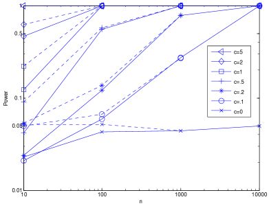
Figure 1: Statistical power of the asymptotic (solid line) and E-divisive (dotted line) methods for detecting change $c$ in mean in a Gaussian signal of length $n$. The first $n/2$ points are i.i.d. $\mathcal{N}(0,1)$ and the last $n/2$ points i.i.d. $\mathcal{N}(c,1)$. The Type I error is also shown ($c=0$). Results are averaged over 1 000 trials.

For the Type I error, we see that both methods hover around the intended value of .05, except for extremely short signals ($n=10$). As for the statistical power, it increases as $n$ and $c$ increase. Furthermore, the asymptotic method rapidly reaches a similar performance as E-divisive: for $n=10$, E-divisive is better (but still with quite poor power), for $n=100$ the asymptotic method has almost caught up, and somewhere between $n=100$ and $n=1\,000$ the results become essentially identical; the asymptotic method has a slight edge at $n=1\,000$.

Let us now see to what extent our method is able to detect changes in variance and tail shape. We considered Gaussian signals of length $n\in\{10,100,1\,000,10\,000\}$ for which there is a change-point after the $(n/2)$-th point, i.e., the first half of the signal is i.i.d. $\mathcal{N}(0,1)$ and the second half either i.i.d. $\mathcal{N}(0,\sigma^{2})$ for $\sigma^{2}\in\{2,5,10\}$ or i.i.d. Student’s $t_{v}$ distributions with $v\in\{2,8,16\}$. Results were averaged over 1 000 trials and are shown in Figure 2.

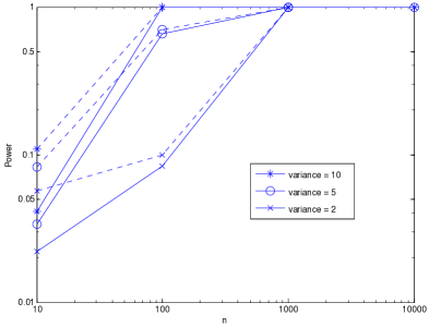
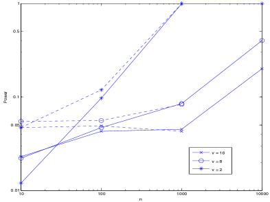
Figure 2: Statistical power of the asymptotic method (solid line) and E-divisive method (dotted line) for detecting change in variance (left) and tail (right) in a signal of length $n$. The first $n/2$ points are i.i.d. $\mathcal{N}(0,1)$ and the last $n/2$ points either i.i.d. $\mathcal{N}(0,\sigma^{2})$, $\sigma^{2}\in\{2,5,10\}$ (left) or from a Student’s $t_{v}$ distribution with $v$ degrees of freedom, $v\in\{2,8,16\}$ (right). Results are averaged over 1 000 trials.

As before, the statistical power tends to increase as $n$ increases and either $\sigma^{2}$ increases or $v$ decreases. The asymptotic method matches or beats the performance of E-divisive starting somewhere between $n=100$ and $n=1\,000$.

Next, we take a look at the performance of the algorithm when the change-point location moves closer to the boundary. As an illustrative example, we work with sequences of length 1 000 and either place the change-point after the 100th, 300th or 500th point. Figure 3 shows histograms of 1 000 repetitions for the predicted location of the change-point, here a change in mean of $c=0.5$ (hardest), $c=1$ (medium) and $c=2$ (easiest).

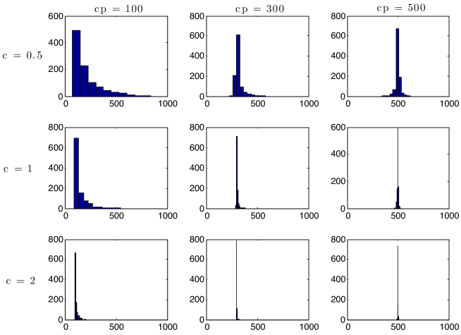
Figure 3: Detecting change in mean of $c=0.5,1$ or $2$ located at different distances to the boundary (change-point location $\mbox{cp}=100,300,500$) in standardized Gaussian signals with 1 000 points. Plots show histograms of predicted change-point location over 1 000 trials.

We see that moving towards the boundary increases the variance and bias in the prediction. However, as the problem becomes easier (bigger jump in mean), both the variance and bias decrease. Similar results are found when looking at change in variance and tail distribution.

II.   Algorithm for long signals

Remember that as it currently stands, the longest signal that we can treat depends on the largest matrix that can be stored, which depends in turn on the memory of a given computer (memory problems for simply manipulating a matrix on a standard PC typically start to occur around $n=10\,$-$15\,000$). For this reason, we now propose a modified algorithm that can treat vastly longer signals.

Long-signal algorithm

1. Extract sub-signal of equidistant points of length 2 000.

2. Run the one change-point algorithm on this. If the null hypothesis is rejected, output the index $k$ of the predicted change-point in this sub-signal. Otherwise, state that no change-point was found.

3. If a change-point was indeed predicted, get the location $k^{\prime}$ in the original signal corresponding to $k$ in the sub-signal and repeat step 1 of the one change-point algorithm in the interval $[k^{\prime}-z,\ k^{\prime}+z]$ to refine the prediction, where $z$ is user-chosen. If $\ell$ is the length of the interval between sub-signal points, one possibility is $z:=\min(2\ell,1\,000)$, where the 1 000 simply ensures this refining step receives a computationally feasible signal length of at most 2 000 points.

We tested this strategy on simulated standard Gaussian signals of length $10^{3},10^{4},10^{5},10^{6}$ and $10^{7}$ with one change-point at the midpoint, a jump of $1$ in the mean. Figure 4 (left) shows the time required to locate the potential change-point.

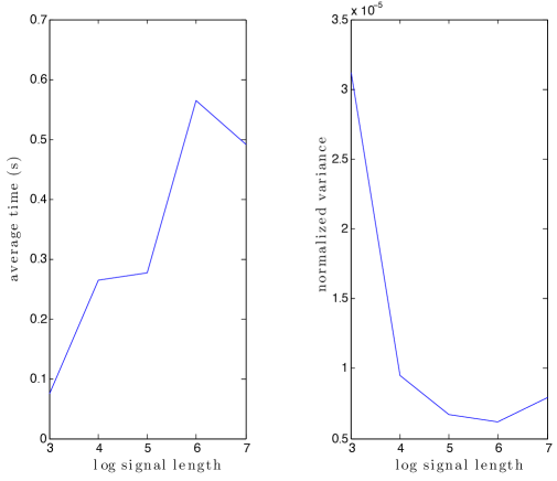
Figure 4: Long-signal change-point detection. Left: Computing time for signals with 1 000 to 10 million points. Right: Variance in first change-point prediction over 1 000 trials after scaling signals to the interval $[0,1]$.

Clearly, this is rapid for even extremely long signals. Looking at the algorithm, we see that it merely involves finding a change-point twice, once in the sub-signal, then once in a contiguous block of the original signal of at most length 2 000. As these two tasks are extremely rapid, the increase in computation time seen mostly comes from the computing overhead of having to extract the sub-signal from longer and longer vectors in memory. In Figure 4 (right), we plot the log signal length against the normalized variance, which means that we calculate the variance in predicted change-point location over 1 000 trials after first dividing the predictions by the length of the signal. Thus all transformed predictions are in the interval $[0,1]$ before their variance is taken. This shows that relative to the length of the signal, subsampling does not deteriorate the change-point prediction quality. Instead, what deteriorates due to subsampling is the absolute prediction quality, i.e., the variance in predicted change-point location does increase as the signal length increases. However, we cannot get around this without introducing significantly more sophisticated subsampling procedures, beyond the scope of the work here.

V.   Discussion

We have derived the asymptotic distribution of a statistic that was previously used to build algorithms for finding change-points in signals. Our new result led to a novel way to construct a practical algorithm for general change-point detection in long signals, which came from the surprising realization that it was possible to approximately simulate from this quite complicated asymptotic distribution. Furthermore, the method appears to have higher power (in the statistical sense) than previous methods based on permutation tests for signals of a thousand points or more. We tested the algorithm on several simulated data sets, as well as a subsampling variant for dealing with extremely long signals.

An interesting line of future research would be to find ways to segment the original signal without requiring stocking a matrix in memory with the same number of rows and columns as there are points in the signal, currently a bottleneck for our approach and even more so for previous permutation approaches. Furthermore, the pertinent choice of the power $\beta\in(0,2)$ remains an open question. Lastly, theoretically valid and experimentally feasible extensions of this framework to the multiple change-point case could be a fruitful line of future research.

VI.   Proof of Theorem II.1

To prove Theorem II.1, we require a useful technical result. Let us begin with some notation. For each integer $K\geq 1$, let $D^{K}[0,1]$ denote the space of bounded measurable functions defined on $[0,1]$ taking values in $\mathbb{R}^{K}$ that are right-continuous with left-hand limits. For each integer $n\geq 1$, let $\mathbb{V}_{n}^{(k)}$, $k\geq 1$, be a sequence of processes taking values in $D^{1}[0,1]$ such that for some $M>0$, uniformly in $k\geq 1$ and $n\geq 1$,

$$\mathbb{E}\left(\sup_{t\in[0,1]}\left|\mathbb{V}_{n}^{(k)}(t)\right|\right)\leq M.$$ (14)

For each integer $K\geq 1$, define the process taking values in $D^{K}[0,1]$ by

$$\mathbb{V}_{n,K}=\left(\mathbb{V}_{n}^{(1)},\ldots,\mathbb{V}_{n}^{(K)}\right).$$

Assume that for each integer $K\geq 1$, $\mathbb{V}_{n,K}$ converges weakly as $n\rightarrow\infty$ to the $D^{K}[0,1]$–valued process $\mathbb{V}_{K}$ defined as

$$\mathbb{V}_{K}:=\left(\mathbb{V}^{(1)},\ldots,\mathbb{V}^{(K)}\right),$$

where $\mathbb{V}^{(k)}$, $k\geq 1,$ is a sequence of $D^{1}[0,1]$–valued processes such that for some $M>0$, uniformly in $k\geq 1$,

$$\mathbb{E}\left(\sup_{t\in[0,1]}\left|\mathbb{V}^{(k)}(t)\right|\right)\leq M.$$ (15)

We shall establish the following useful result.

Proposition VI.1

With the notation and assumptions introduced above, for any choice of constants $a_{m}$, $m\geq 1$, satisfying $\sum_{m=1}^{\infty}|a_{m}|<\infty$, the sequence of $D^{1}[0,1]$–valued processes

$$T_{n}:=\sum_{m=1}^{\infty}a_{m}\mathbb{V}_{n}^{(m)}$$

converges weakly in $D^{1}[0,1]$ to the $D^{1}[0,1]$–valued process

$$T:=\sum_{m=1}^{\infty}a_{m}\mathbb{V}^{(m)}.$$

Proof.  Notice that by (14)

$$\mathbb{E}\left(\sum_{m=1}^{\infty}\left|a_{m}\right|\sup_{t\in[0,1]}\left|\mathbb{V}_{n}^{(m)}(t)\right|\right)\leq M\sum_{m=1}^{\infty}|a_{m}|<\infty.$$

From this we get that with probability $1$, for each $n\geq 1$,

$$\sum_{m=1}^{\infty}\left|a_{m}\right|\sup_{t\in[0,1]}\left|\mathbb{V}_{n}^{(m)}(t)\right|<\infty,$$

which in turn implies that with probability $1$, for each $n\geq 1$,

$$\lim_{K\rightarrow\infty}\sup_{t\in[0,1]}\left|\overline{T}_{n}^{(K)}(t)\right|=0,$$ (16)

where

$$\overline{T}_{n}^{(K)}(t):=\sum_{m=K+1}^{\infty}a_{m}\mathbb{V}_{n}^{(m)}(t).$$

Since for each $n\geq 1$ and $K\geq 1$, $T_{n}^{(K)}\in D^{1}[0,1]$, where $T_{n}^{(K)}:=\sum_{m=1}^{K}a_{m}\mathbb{V}_{n}^{(m)}$, by completeness of $D^{1}[0,1]$ in the supremum metric (see page 150 of monograph [2]), we infer that $T_{n}\in D^{1}[0,1]$. In the same way we get using (15) that

$$\lim_{K\rightarrow\infty}\sup_{t\in[0,1]}\left|\overline{T}^{(K)}(t)\right|=0,$$ (17)

where

$$\overline{T}^{(K)}(t):=\sum_{m=K+1}^{\infty}a_{m}\mathbb{V}^{(m)}(t),$$

and thus that $T\in D^{1}[0,1]$. Also, since by assumption for each integer $K\geq 1$, $\mathbb{V}_{n,K}$ converges weakly as $n\rightarrow\infty$ to the $D^{K}[0,1]$–valued process $\mathbb{V}_{K}$, we get that $T_{n}^{(K)}$ converges weakly in $D^{1}[0,1]$ to $T^{(K)}$, where

$$T_{n}^{(K)}:=\sum_{m=1}^{K}a_{m}\mathbb{V}_{n}^{(m)}\quad\text{ and }\quad T^{(K)}:=\sum_{m=1}^{K}a_{m}\mathbb{V}^{(m)}.$$

We complete the proof by combining this with (16) and (17), and then appealing to Theorem 4.2 of [2]. $\quad\square$

We are now ready to prove Theorem II.1. It turns out that it is more convenient to prove the result for the following version of the process $\mathbb{Y}_{n}$, namely

$$\tilde{\mathbb{Y}}_{n}(\tilde{h}_{2},t):=\frac{2\lfloor nt\rfloor\left(n-\lfloor nt\rfloor\right)}{n^{3}}U_{n}(\tilde{h}_{2})-\frac{2\left(n-\lfloor nt\rfloor\right)}{n^{2}}U_{\lfloor nt\rfloor}^{(1)}(\tilde{h}_{2})-\frac{2\lfloor nt\rfloor}{n^{2}}U_{\lfloor nt\rfloor}^{(2)}(\tilde{h}_{2}),$$

which is readily shown to be asymptotically equivalent to $\mathbb{Y}_{n}(\tilde{h}_{2},t)$. Following pages 196-197 of [21], we see that

$$\frac{2U_{n}(\tilde{h}_{2})}{n}=\sum_{k=1}^{\infty}\lambda_{k}\left[\left(\sum_{i=1}^{n}\phi_{k}(X_{i})/\sqrt{n}\right)^{2}-\frac{1}{n}\sum_{i=1}^{n}\phi_{k}^{2}(X_{i})\right]=:\sum_{k=1}^{\infty}\lambda_{k}\Delta_{k,n},$$

$$\frac{2U_{\lfloor nt\rfloor,n}^{(1)}(\tilde{h}_{2})}{n}=\sum_{k=1}^{\infty}\lambda_{k}\left[\left(\sum_{i=1}^{\lfloor nt\rfloor}\phi_{k}(X_{i})/\sqrt{n}\right)^{2}-\frac{1}{n}\sum_{i=1}^{\lfloor nt\rfloor}\phi_{k}^{2}(X_{i})\right]=:\sum_{k=1}^{\infty}\lambda_{k}\Delta_{k,n}^{(1)}(t),$$

and

$$\frac{2U_{\lfloor nt\rfloor,n}^{(2)}(\tilde{h}_{2})}{n}=\sum_{k=1}^{\infty}\lambda_{k}\left[\left(\sum_{i=1+\lfloor nt\rfloor}^{n}\phi_{k}(X_{i})/\sqrt{n}\right)^{2}-\frac{1}{n}\sum_{i=1+\lfloor nt\rfloor}^{n}\phi_{k}^{2}(X_{i})\right]=:\sum_{k=1}^{\infty}\lambda_{k}\Delta_{k,n}^{(2)}(t).$$

Thus,

$$\tilde{\mathbb{Y}}_{n}(\tilde{h}_{2},t)=\sum_{k=1}^{\infty}\lambda_{k}\left(\frac{\lfloor nt\rfloor\left(n-\lfloor nt\rfloor\right)}{n^{2}}\Delta_{k,n}-\frac{\left(n-\lfloor nt\rfloor\right)}{n}\Delta_{k,n}^{(1)}(t)-\frac{\lfloor nt\rfloor}{n}\Delta_{k,n}^{(2)}(t)\right)=:\sum_{k=1}^{\infty}\lambda_{k}\mathbb{V}_{n}^{(k)}(t).$$ (18)

Let $\{\mathbb{W}^{(i)}\}_{i\geq 1}$ be a sequence of standard Wiener processes on $\left[0,1\right]$. Write

$$\mathbb{Y}(t):=\sum_{k=1}^{\infty}\lambda_{k}\mathbb{V}^{(k)}(t),$$

where, for $k\geq 1$,

$$\mathbb{V}^{(k)}(t) =t(1-t)\left(\left(\mathbb{W}^{(k)}(1)\right)^{2}-1\right)-(1-t)\left(\left(\mathbb{W}^{(k)}(t)\right)^{2}-t\right)$$

$$\quad-t\left(\left(\mathbb{W}^{(k)}(1)-\mathbb{W}^{(k)}(t)\right)^{2}-(1-t)\right)$$

$$=t(1-t)\left(\left(\mathbb{W}^{(k)}(1)\right)^{2}+1\right)-(1-t)\left(\mathbb{W}^{(k)}(t)\right)^{2}-t\left(\mathbb{W}^{(k)}(1)-\mathbb{W}^{(k)}(t)\right)^{2}.$$ (19)

A simple application of Doob’s inequality shows that there exists a constant $M>0$ such that (14) and (15) hold, for $\mathbb{V}_{n}^{(k)}$ and $\mathbb{V}^{(k)}$ defined as in (18) and (19).

For any integer $K\geq 1$, let $\mathbb{U}_{1}$ be the random vector such that $\mathbb{U}_{1}^{T}=(\phi_{1}(X_{1}),\ldots,\phi_{K}(X_{1}))$. We see that $\mathbb{E}(\mathbb{U}_{1})=\mathbf{0}$ and $\mathbb{E}(\mathbb{U}_{1}\mathbb{U}_{1}^{T})=I_{K}$. For any $n\geq 1$ let $\mathbb{U}_{1},\ldots,\mathbb{U}_{n}$ be i.i.d. $\mathbb{U}_{1}$. Consider the process defined on $D^{K}[0,1]$ by

$$\mathbb{W}_{n,K}(t):=\left(n^{-1/2}\sum_{j\leq\lfloor nt\rfloor}\phi_{1}(X_{j}),\ldots,n^{-1/2}\sum_{j\leq\lfloor nt\rfloor}\phi_{K}(X_{j})\right)=:\left(\mathbb{W}_{n}^{(1)}(t),\ldots,\mathbb{W}_{n}^{(K)}(t)\right),$$

where for any $i\geq 1$,

$$\mathbb{W}_{n}^{(i)}(t):=n^{-1/2}\sum_{j\leq\lfloor nt\rfloor}\phi_{i}(X_{j}).$$

Notice that as processes in $t\in[0,1]$,

$$\mathbb{W}_{n,K}(t):\overset{\mathrm{D}}{=}n^{-1/2}\sum_{j\leq\lfloor nt\rfloor}\mathbb{U}_{j}.$$

Clearly by Donsker’s theorem the process $(\mathbb{W}_{n,K}(t))_{0\leq t\leq 1}$ converges weakly as $n\rightarrow\infty$ to the $\mathbb{R}^{K}$–valued Wiener process $(\mathbb{W}_{K}(t))_{0\leq t\leq 1},$ with mean vector zero and covariance matrix $(t_{1}\wedge t_{2})I_{K}$, $t_{1},t_{2}\in[0,1]$, where

$$\mathbb{W}_{K}(t):=\left(\mathbb{W}^{(1)}(t),\ldots,\mathbb{W}^{(K)}(t)\right).$$

Using this fact along with the law of large numbers one readily verifies that for each integer $K\geq 1$, $(\mathbb{V}_{n}^{(1)},\ldots,\mathbb{V}_{n}^{(K)})$ converges weakly as $n\rightarrow\infty$ to $(\mathbb{V}^{(1)},\ldots,\mathbb{V}^{(K)})$, where $\mathbb{V}_{n}^{(i)}$ and $\mathbb{V}^{(i)}$ are defined as in (18) and (19). All the conditions for Proposition VI.1 to hold have been verified. Thus the proof of Theorem II.1 is complete, after we note that a little algebra shows that $\mathbb{Y}(t)$ is equal to

$$\sum_{i=1}^{\infty}\lambda_{i}\left(t(1-t)-\left(\mathbb{W}^{(i)}(t)-t\mathbb{W}^{(i)}(1)\right)^{2}\right)=\sum_{i=1}^{\infty}\lambda_{i}\left(t(1-t)-\left(\mathbb{B}^{(i)}(t)\right)^{2}\right),$$

where $\mathbb{B}^{(i)}(t)=\mathbb{W}^{(i)}(t)-t\mathbb{W}^{(i)}(1)$, $i\geq 1$, are independent Brownian bridges.$\quad\square$

VII.   Appendix

I.   Proof of Lemma II.1

Notice that for each $n>1$, $\mathcal{E}_{\left\lfloor n\gamma\right\rfloor,n}({\bf X};\beta)$ is equal to the statistic in (3) with $k=\left\lfloor n\gamma\right\rfloor$.  By the law of large numbers for U-statistics (see Theorem 1 of [20]) for any $\gamma\in(0,1)$, with probability 1,

$${\binom{\left\lfloor n\gamma\right\rfloor}{2}}^{-1}\sum_{1\leq i<j\leq\left\lfloor n\gamma\right\rfloor}\left|Y_{i}-Y_{j}\right|^{\beta}\rightarrow\mathbb{E}\left|Y-Y^{\prime}\right|^{\beta}$$

and

$${\binom{n-\left\lfloor n\gamma\right\rfloor}{2}}^{-1}\sum_{1\leq i<j\leq n-\left\lfloor n\gamma\right\rfloor}\left|Z_{i}-Z_{j}\right|^{\beta}\rightarrow\mathbb{E}\left|Z-Z^{\prime}\right|^{\beta}.$$

Next for any $M>0$, write

$$\left|y-z\right|^{\beta} =\left|y-z\right|^{\beta}1\left\{\left|y\right|\leq M,\left|z\right|\leq M\right\}+\left|y-z\right|^{\beta}1\left\{\left|y\right|\leq M,\left|z\right|>M\right\}$$

$$\quad+\left|y-z\right|^{\beta}1\left\{\left|y\right|>M,\left|z\right|\leq M\right\}+\left|y-z\right|^{\beta}1\left\{\left|y\right|>M,\left|z\right|>M\right\}.$$

Applying the strong law of large numbers for generalized U-statistics given in Theorem 1 of [20], we get for any $M>0$, with probability 1,

$$\frac{2}{\left\lfloor n\gamma\right\rfloor(n-\left\lfloor n\gamma\right\rfloor)}\sum_{i=1}^{\left\lfloor n\gamma\right\rfloor}\sum_{j=1}^{n-\left\lfloor n\gamma\right\rfloor}\left|Y_{i}-Z_{j}\right|^{\beta}1\left\{\left|Y_{i}\right|\leq M,\left|Z_{j}\right|\leq M\right\}$$

$$\quad\rightarrow 2\mathbb{E}\left(\left|Y-Z\right|^{\beta}1\left\{\left|Y\right|\leq M,\left|Z\right|\leq M\right\}\right).$$

Also observe that

$$\frac{2}{\left\lfloor n\gamma\right\rfloor(n-\left\lfloor n\gamma\right\rfloor)}\sum_{i=1}^{\left\lfloor n\gamma\right\rfloor}\sum_{j=1}^{n-\left\lfloor n\gamma\right\rfloor}\left|Y_{i}-Z_{j}\right|^{\beta}1\left\{\left|Y_{i}\right|\leq M,\left|Z_{j}\right|>M\right\}$$

$$\quad\leq\frac{2}{\left\lfloor n\gamma\right\rfloor(n-\left\lfloor n\gamma\right\rfloor)}\sum_{i=1}^{\left\lfloor n\gamma\right\rfloor}\sum_{j=1}^{n-\left\lfloor n\gamma\right\rfloor}\left(M+\left|Z_{j}\right|\right)^{\beta}1\left\{\left|Z_{j}\right|>M\right\}$$

$$\quad=\frac{2}{n-\left\lfloor n\gamma\right\rfloor}\sum_{j=1}^{n-\left\lfloor n\gamma\right\rfloor}\left(M+\left|Z_{j}\right|\right)^{\beta}1\left\{\left|Z_{j}\right|>M\right\}.$$

By the usual law of large numbers for each $M>0$, with probability 1,

$$\frac{2}{n-\left\lfloor n\gamma\right\rfloor}\sum_{j=1}^{n-\left\lfloor n\gamma\right\rfloor}\left(M+\left|Z_{j}\right|\right)^{\beta}1\left\{\left|Z_{j}\right|>M\right\} \rightarrow 2\mathbb{E}\left(\left(M+\left|Z\right|\right)^{\beta}1\left\{\left|Z\right|>M\right\}\right)$$

$$\leq 2^{\beta+1}\mathbb{E}\left(\left|Z\right|^{\beta}1\left\{\left|Z\right|>M\right\}\right).$$

Thus, with probability 1, for all $M>0$,

$$\limsup_{n\rightarrow\infty}\frac{2}{\left\lfloor n\gamma\right\rfloor(n-\left\lfloor n\gamma\right\rfloor)}\sum_{i=1}^{\left\lfloor n\gamma\right\rfloor}\sum_{j=1}^{n-\left\lfloor n\gamma\right\rfloor}\left|Y_{i}-Z_{j}\right|^{\beta}1\left\{\left|Y_{i}\right|\leq M,\left|Z_{j}\right|>M\right\}$$

$$\quad\leq 2^{\beta+1}\mathbb{E}\left(\left|Z\right|^{\beta}1\left\{\left|Z\right|>M\right\}\right).$$

In the same way we get that, with probability 1,

$$\limsup_{n\rightarrow\infty}\frac{2}{\left\lfloor n\gamma\right\rfloor(n-\left\lfloor n\gamma\right\rfloor)}\sum_{i=1}^{\left\lfloor n\gamma\right\rfloor}\sum_{j=1}^{n-\left\lfloor n\gamma\right\rfloor}\left|Y_{i}-Z_{j}\right|^{\beta}1\left\{\left|Y_{i}\right|>M,\left|Z_{j}\right|\leq M\right\}$$

$$\quad\leq 2\mathbb{E}\left(\left(\left|Y\right|+M\right)^{\beta}1\left\{\left|Y\right|>M\right\}\right)\leq 2^{\beta+1}\mathbb{E}\left(\left|Y\right|^{\beta}1\left\{\left|Y\right|>M\right\}\right).$$

Finally, note that, by the $c_{r}$-inequality,

$$\frac{2}{\left\lfloor n\gamma\right\rfloor(n-\left\lfloor n\gamma\right\rfloor)}\sum_{i=1}^{\left\lfloor n\gamma\right\rfloor}\sum_{j=1}^{n-\left\lfloor n\gamma\right\rfloor}\left|Y_{i}-Z_{j}\right|^{\beta}1\left\{\left|Y_{i}\right|>M,\left|Z_{j}\right|>M\right\}$$

$$\quad\leq\frac{2^{\beta}}{\left\lfloor n\gamma\right\rfloor(n-\left\lfloor n\gamma\right\rfloor)}\sum_{i=1}^{\left\lfloor n\gamma\right\rfloor}\sum_{j=1}^{n-\left\lfloor n\gamma\right\rfloor}\left(\left|Y_{i}\right|^{\beta}+\left|Z_{j}\right|^{\beta}\right)1\left\{\left|Y_{i}\right|>M,\left|Z_{j}\right|>M\right\}$$

$$\quad\leq\frac{2^{\beta}}{\left\lfloor n\gamma\right\rfloor}\sum_{i=1}^{\left\lfloor n\gamma\right\rfloor}\left|Y_{i}\right|^{\beta}1\left\{\left|Y_{i}\right|>M\right\}+\frac{2^{\beta}}{n-\left\lfloor n\gamma\right\rfloor}\sum_{j=1}^{n-\left\lfloor n\gamma\right\rfloor}\left|Z_{j}\right|^{\beta}1\left\{\left|Z_{j}\right|>M\right\}.$$

By the law of large numbers this converges, with probability 1, to

$$2^{\beta}\mathbb{E}\left(\left|Y\right|^{\beta}1\left\{\left|Y\right|>M\right\}\right)+2^{\beta}\mathbb{E}\left(\left|Z\right|^{\beta}1\left\{\left|Z\right|>M\right\}\right).$$

Obviously as $M\rightarrow\infty$,

$$2\mathbb{E}\left(\left|Y-Z\right|^{\beta}1\left\{\left|Y\right|\leq M,\left|Z\right|\leq M\right\}\right)\rightarrow 2\mathbb{E}\left|Y-Z\right|^{\beta}$$

and

$$3\cdot 2^{\beta}\mathbb{E}\left(\left|Y\right|^{\beta}1\left\{\left|Y\right|>M\right\}\right)+3\cdot 2^{\beta}\mathbb{E}\left(\left|Z\right|^{\beta}1\left\{\left|Z\right|>M\right\}\right)\rightarrow 0.$$

Putting everything together we get that (13) holds. $\quad\square$

II.   A technical result

Let $X$ and $X^{\prime}$ be i.i.d. $F$ and let $\varphi$ be a symmetric measurable function from $\mathbb{R}^{d}\times\mathbb{R}^{d}\rightarrow\mathbb{R}$ such that $\mathbb{E}\varphi^{2}(X,X^{\prime})<\infty$. Recall the notation (6). Let $A$ be the operator defined on $L_{2}(\mathbb{R}^{d},F)$ as in (8).

Notice that

$$\mathbb{E}\big{(}g(X)\tilde{h}_{2}(X,X^{\prime})g(X^{\prime})\big{)}=\int_{\mathbb{R}^{d}}g(x)Ag(x)dF(x)=:\langle g,Ag\rangle.$$

Let us now introduce some useful definitions. Given $\beta\in(0,2)$ and $\varphi_{\beta}(x,y)=|x-y|^{\beta}$, define as in (6),

$$h_{2,\beta}(x,y)=\varphi_{\beta}(x,y)-\varphi_{1,\beta}(x)-\varphi_{1,\beta}(y)\quad\text{ and }\quad\tilde{h}_{2,\beta}(x,y)=h_{\beta}(x,y)+\mathbb{E}\varphi_{\beta}(X,X^{\prime}).$$

The aim here is to verify that the function $\tilde{h}_{2,\beta}(x,y)$ satisfies the conditions of Theorem II.1 as long as

$$\mathbb{E}|X|^{2\beta}<\infty.$$ (20)

Let $\tilde{A}_{\beta}$ denote the integral operator

$$\tilde{A}_{\beta}g(x)=\int_{\mathbb{R}^{d}}\text{ }\tilde{h}_{2,\beta}(x,y)g(y)dF(y),\quad x\in\mathbb{R}^{d},\text{ }g\in L_{2}(\mathbb{R}^{d},F).$$

Clearly (20) implies (5) with $\varphi=\varphi_{\beta}$, which, in turn, by (9) implies

$$\mathbb{E}\tilde{h}_{2,\beta}^{2}(X,X^{\prime})=\int_{\mathbb{R}^{d}}\int_{\mathbb{R}^{d}}\tilde{h}_{2,\beta}^{2}(x,y)dF(x)dF(y)=\sum_{i=1}^{\infty}\lambda_{i}^{2}<\infty,$$

where $\lambda_{i}$, $i\geq 1$, are the eigenvalues of the operator $\tilde{A}_{\beta}$, with corresponding orthonormal eigenfunctions $\phi_{i}$, $i\geq 1$.

Next we shall prove that when (20) holds then the eigenvalues $\lambda_{i}$, $i\geq 1$, of this integral operator $\tilde{A}_{\beta}$ satisfy (10). This is summarized in the following lemma, whose proof is postponed to the next paragraph.

Lemma VII.1

Whenever for some $\beta\in(0,2)$, (20) holds, the eigenvalues $\lambda_{i}$, $i\geq 1$, of the operator $\tilde{A}_{\beta}$ satisfy (10).

The technical results that follow will imply that $\lambda_{i}\leq 0$ for all $i\geq 1$ and $\sum_{i=1}^{\infty}\lambda_{i}$ is finite, from which we can infer (10), and thus Lemma VII.1. Let us begin with two definitions.

Definition VII.1

Let $\mathcal{X}$ be a nonempty set. A symmetric function $K:\mathcal{X}\times\mathcal{X}\rightarrow\mathbb{R}$ is called positive definite if

$$\sum_{i=1}^{n}\sum_{j=1}^{n}c_{i}c_{j}K(x_{i},x_{j})\geq 0$$

for all $n\geq 1$, $c_{1},\ldots,c_{n}\in\mathbb{R}$ and $x_{1},\ldots,x_{n}\in\mathcal{X}$.

Definition VII.2

Let $\mathcal{X}$ be a nonempty set. A symmetric function $K:\mathcal{X}\times\mathcal{X}\rightarrow\mathbb{R}$ is called conditionally negative definite if

$$\sum_{i=1}^{n}\sum_{j=1}^{n}c_{i}c_{j}K(x_{i},x_{j})\leq 0$$

for all $n\geq 1$, $c_{1},\ldots,c_{n}\in\mathbb{R}$ such that  $\sum_{i=1}^{n}c_{i}=0$ and $x_{1},\ldots,x_{n}\in\mathcal{X}$.

Next, we shall be using part of Lemma 2.1 on page 74 of [1], which we state here for convenience as Lemma VII.2.

Lemma VII.2

Let $K$ be a symmetric function on $\mathcal{X}\times\mathcal{X}$. Then, for any $x_{0}\in\mathcal{X}$, the function

$$\tilde{K}(x,y)=K(x,x_{0})+K(y,x_{0})-K(x,y)-K(x_{0},x_{0})$$

is positive definite if and only if $K$ is conditionally negative definite.

The following lemma can be proved just as Corollary 2.1 in [8].

Lemma VII.3

Let $H:\mathbb{R}^{d}\times\mathbb{R}^{d}$ $\rightarrow\mathbb{R}$ be a symmetric positive definite function in the sense of Definition VII.1. Assume that $H$ is continuous and $\mathbb{E}H^{2}(X,X^{\prime})<\infty,$ where $X$ and $X^{\prime}$ are i.i.d. $F$. Then $\mathbb{E}(g(X)H(X,X^{\prime})g(X^{\prime}))\geq 0$ for all $g\in L_{2}(\mathbb{R}^{d},F)$, i.e., $H$ is $L^{2}$-positive definite in the sense of [8].

We recall that an operator $L$ on $L_{2}(\mathbb{R}^{d},F)$ is called positive definite if for all $g\in L_{2}(\mathbb{R}^{d},F)$, $\langle g,Lg\rangle\geq 0$.

Proposition VII.1

Let $\varphi:\mathbb{R}^{d}\times\mathbb{R}^{d}\rightarrow\mathbb{R}$ be a symmetric continuous function that is a conditionally negative definite function in the sense of Definition VII.2. Assume that $\varphi(x,x)=0$ for all $x\in\mathbb{R}^{d}$ and $\mathbb{E}\varphi^{2}(X,X^{\prime})<\infty$. Then $\varphi$ defines a positive definite operator $L$ on $L_{2}(\mathbb{R}^{d},F)$ given by

$$Lg(x)=-\int_{\mathbb{R}^{d}}h(x,y)g(y)dF(y),\quad x\in\mathbb{R}^{d},g\in L_{2}(\mathbb{R}^{d},F),$$

where $h$ is defined as in (6). Furthermore the operator $\tilde{L}$ on $L_{2}(\mathbb{R}^{d},F)$ given by

$$\tilde{L}g(x)=-\int_{\mathbb{R}^{d}}\left(h(x,y)+\mathbb{E}\varphi(X,X^{\prime})\right)g(y)dF(y),\quad x\in\mathbb{R}^{d},g\in L_{2}(\mathbb{R}^{d},F),$$

is also a positive definite operator on $L_{2}(\mathbb{R}^{d},F)$.

Proof. We must show that for all $g\in L_{2}(\mathbb{R}^{d},F)$,

$$\langle g,Lg\rangle=-\mathbb{E}(g(X)h(X,X^{\prime})g(X^{\prime}))\geq 0.$$

For any $u\in\mathbb{R}^{d}$, let us write

$$\varphi(x,y,u) :=\varphi(x,u)+\varphi(y,u)-\varphi(u,u)-\varphi(x,y)$$

$$=\varphi(x,u)+\varphi(y,u)-\varphi(x,y).$$

Since $\varphi$ is assumed to be conditionally negative definite, by Lemma VII.2 we have that for any fixed $u\in\mathbb{R}^{d}$, $\varphi(x,y,u)$ is positive definite in the sense of Definition VII.1. Hence, since $\varphi$ is also assumed to be continuous, by Lemma VII.3 for all $g\in L_{2}(\mathbb{R}^{d},F)$,

$$\mathbb{E}\left(g(X)\varphi(X,X^{\prime},u)g(X^{\prime})\right)\geq 0.$$

Noting that if $U$ has distribution function $F$, $\mathbb{E}\varphi(x,y,U)=-h(x,y)$, we get, assuming that $X$, $X^{\prime}$ and $U$ are independent, that

$$\mathbb{E}\left(g(X)\varphi(X,X^{\prime},U)g(X^{\prime})\right)=-\mathbb{E}\left(g(X)h(X,X^{\prime})g(X^{\prime})\right)\geq 0.\qquad$$

Next, notice that for any eigenvalue and normalized eigenfunction $(\tilde{\lambda}_{i},\tilde{\phi}_{i})$ pair, $i\geq 1$, of the operator $\tilde{L}$, we have

$$\tilde{\lambda}_{i}\tilde{\phi}_{i}(x)=\tilde{L}\tilde{\phi}_{i}(x)=-\int_{\mathbb{R}^{d}}\left(h(x,y)+\mathbb{E}\varphi(X,X^{\prime})\right)\tilde{\phi}_{i}\left(y\right)dF(y).$$

Now,

$$\int_{\mathbb{R}^{d}}\left(h(x,y)+\mathbb{E}\varphi(X,X^{\prime})\right)dF(y)=0\text{, for all }x\in\mathbb{R}^{d},$$

implies that $(\tilde{\lambda}_{1},\tilde{\phi}_{1}):=\left(0,1\right)$ is an eigenvalue and normalized eigenfunction pair of $\tilde{L}$. From this we get that whenever $\tilde{\lambda}_{i}\neq 0$, $\mathbb{E}\tilde{\phi}_{i}(X)=0$, $i\geq 2$, which says that for such $\tilde{\lambda}_{i}$,

$$\tilde{\lambda}_{i}\tilde{\phi}_{i}(x)=-\int_{\mathbb{R}^{d}}h(x,y)\tilde{\phi}_{i}(y)dF(y).$$

This implies that whenever for some $i\geq 1,$ $(\tilde{\lambda}_{i},\tilde{\phi}_{i})$, with $\tilde{\lambda}_{i}\neq 0,$ is an eigenvalue and normalized eigenfunction pair of the operator $\tilde{L},$ it is also an eigenvalue and normalized eigenfunction pair of the operator $L$. Moreover, since the integral operator $L$ is positive definite on $L_{2}(\mathbb{R}^{d},F)$, this implies that for any such nonzero $\tilde{\lambda}_{i}$ (where necessarily $i\geq 2$)

$$-\int_{\mathbb{R}^{d}}\int_{\mathbb{R}^{d}}\tilde{\phi}_{i}(x)\left(h(x,y)+\mathbb{E}\varphi(X,X^{\prime})\right)\tilde{\phi}_{i}(y)dF(x)dF(y)$$

$$\quad=-\int_{\mathbb{R}^{d}}\int_{\mathbb{R}^{d}}\tilde{\phi}_{i}(x)h(x,y)\tilde{\phi}_{i}(y)dF(x)dF(y)=\tilde{\lambda}_{i}\geq 0,$$

which says that the operator $\tilde{L}$ is positive definite on $L_{2}(\mathbb{R}^{d},F)$. $\quad\square$

III.   Proof of Lemma VII.1

A special case of Theorem 3.2.2 in [1] says that the function $\varphi_{\beta}(x,y)=|x-y|^{\beta}$, $\beta\in(0,2)$, is conditionally negative definite. Also see Exercise 3.2.13b in [1] and the discussion after Proposition 3 in [26]. Therefore by Proposition VII.1 the integral operator $L_{\beta}$ defined by the function

$$K_{\beta}\left(x,y\right)=-h_{2,\beta}\left(x,y\right)$$

is positive definite as well as the integral operator $\tilde{L}_{\beta}=-\tilde{A}_{\beta}$ defined by the function

$$\tilde{K}_{\beta}\left(x,y\right)=-h_{2,\beta}(x,y)-\mathbb{E}\varphi_{\beta}(X,X^{\prime}).$$

Next, as in the proof of Proposition VII.1, any eigenvalue and normalized eigenfunction

$$\big{(}\tilde{\lambda}_{i},\tilde{\phi}_{i}\big{)}=\left(-\lambda_{i},-\phi_{i}\right)$$

pair, with $\tilde{\lambda}_{i}\neq 0$, $i\geq 1$, of the operator $\tilde{L}_{\beta}=-\tilde{A}_{\beta}$ is also an eigenvalue and normalized eigenfunction pair of the operator $L_{\beta}$.

We shall apply Theorem 2 of [23] to show that uniformly on compact subsets $D$ of $\mathbb{R}^{d}$,

$$K_{\beta}\left(x,y\right)=\sum_{i=1}^{\infty}\rho_{i}\psi_{i}(x)\psi_{i}(y),\quad\left(x,y\right)\in D\times D,$$

where $\rho_{i}\geq 0$, $i\geq 1$, are the eigenvalues of the operator $L_{\beta}=-A_{\beta}$ with corresponding normalized eigenfunctions $\psi_{i}$, $i\geq 1$. In particular

$$K_{\beta}\left(x,x\right)=\sum_{i=1}^{\infty}\rho_{i}\psi_{i}^{2}(x),\quad x\in D,$$

and thus since $\mathbb{E}\psi_{i}^{2}(X)=1$, $i\geq 1$, and $\mathbb{E}K_{\beta}\left(X,X\right)<\infty$, we get

$$\sum_{i=1}^{\infty}\rho_{i}<\infty.$$

Therefore since, as pointed out above, the eigenvalue and normalized eigenfunction pairs $(-\lambda_{i},-\phi_{i})$ of $\tilde{L}_{\beta}=-\tilde{A}_{\beta}$, with $\lambda_{i}\neq 0$, are also eigenvalue and normalized eigenfunction pairs of the operator $L_{\beta}$ this implies that $\sum_{i=1}^{\infty}|\lambda_{i}|<\infty$.

Our proof will be complete once we have checked that $L_{\beta}$ satisfies the conditions of Theorem 2 of [23].

Since the function $\varphi_{\beta}(x,y)=|x-y|^{\beta}$, $\beta\in(0,2),$ is conditionally negative definite, by Lemma VII.2 the function $K_{\beta}\left(x,y\right)$ is positive definite. To see this note that by Lemma VII.2 for any fixed $u\in\mathbb{R}$ the function

$$\varphi_{\beta}\left(x,u\right)+\varphi_{\beta}\left(u,y\right)-\varphi_{\beta}\left(x,y\right)-\varphi_{\beta}\left(u,u\right)=\varphi_{\beta}\left(x,u\right)+\varphi_{\beta}\left(u,y\right)-\varphi_{\beta}\left(x,y\right)$$

is positive definite. Therefore we readily see that

$$K_{\beta}(x,y)=\left(\int_{\mathbb{R}^{d}}\varphi_{\beta}\left(x,u\right)+\varphi_{\beta}\left(u,y\right)-\varphi_{\beta}\left(x,y\right)\right)dF\left(u\right)$$

is positive definite. In addition, $K_{\beta}\left(x,y\right)$ is symmetric and continuous, and thus $K_{\beta}\left(x,y\right)$ is a Mercer kernel in the terminology of [23]. We must also verify the following assumptions.

Assumption A. For each $x\in\mathbb{R}^{d}$, $K_{\beta}\left(x,\cdot\right)\in L_{2}(\mathbb{R}^{d},F).$

Assumption B. $L_{\beta}$ is a bounded and positive definite operator on $L_{2}(\mathbb{R}^{d},F)$ and for every $g\in L_{2}(\mathbb{R}^{d},F)$, the function

$$L_{\beta}g(x)=\int_{\mathbb{R}^{d}}K_{\beta}(x,y)g(y)dF(y)$$

is a continuous function on $\mathbb{R}^{d}$.

Assumption C. $L_{\beta}$ has at most countably many positive eigenvalues and orthonormal eigenfunctions.

Since $\varphi_{\beta}$ is a symmetric continuous function that is conditionally negative definite in the sense of Definition VII.2 satisfying $\varphi_{\beta}(x,x)=0$ for all $x\in\mathbb{R}^{d}$ and $\mathbb{E}\varphi_{\beta}^{2}(X,X^{\prime})<\infty$, we get by Proposition VII.1 that $L_{\beta}$ is a positive definite operator on $L_{2}(\mathbb{R}^{d},F)$.  Also (20) obviously implies that Assumption A holds and

$$\mathbb{E}K_{\beta}^{2}(X,X^{\prime})=\int_{\mathbb{R}^{d}}\int_{\mathbb{R}^{d}}K_{\beta}^{2}(x,y)dF(x)dF(y)<\infty,$$

which by Proposition 1 of [23] implies that the operator $L_{\beta}$ is bounded and compact. (From Sun’s Proposition 1 one can also infer that $L_{\beta}$ is positive definite. However, he does not provide a proof. Therefore we invoke our Lemma VII.3 here.) An elementary argument based on the dominated convergence theorem implies that $L_{\beta}g(x)$ is a continuous function on $\mathbb{R}^{d}$. Thus Assumption B is satisfied. Finally, since the operator $L_{\beta}$ is compact, Theorem VII.4.5 of [7] implies that Assumption C is fulfilled. Thus the assumptions of Theorem 2 of [23] hold. This completes the proof of Lemma VII.1. $\quad\square$

References

- [1] C. Berg, J. P. R. Christensen, and P. Ressel. Harmonic Analysis on Semigroups. Springer, New York, 1984.
- [2] P. Billingsley. Convergence of Probability Measures. Wiley, New York, 1968.
- [3] R. Bolton and D. Hand. Statistical fraud detection: A review. Statistical Science, 17:235–255, 2002.
- [4] B. P. Carlin, A. E. Gelfand, and A. F. Smith. Hierarchical Bayesian analysis of changepoint problems. Applied Statistics, 41:389–405, 1992.
- [5] M. Csörgő and L. Horváth. Limit Theorems in Change-Point Analysis. Wiley, New York, 1997.
- [6] M. Csörgő and L. Horváth. Invariance principles for changepoint problems. Journal of Multivariate Analysis, 27:151–168, 1988.
- [7] N. Dunford and J. T. Schwartz. Linear Operators. Wiley, New York, 1963.
- [8] J. C. Ferreira and V. A. Menegatto. Eigenvalues of integral operators defined by smooth positive definite kernels. Integral Equations and Operator Theory, 64:61–81, 2009.
- [9] W. Hoeffding. A class of statistics with asymptotically normal distribution. The Annals of Mathematical Statistics, 19:293–325, 1948.
- [10] W. Hoeffding. The large-sample power of tests based on permutations of observations. The Annals of Mathematical Statistics, 23:169–192, 1952.
- [11] A. Kim, C. Marzban, D. Percival, and W. Stuetzie. Using labeled data to evaluate change detectors in a multivariate streaming environment. Signal Processing, 89:2529–2536, 2009.
- [12] V. Koltchinskii and E. Giné. Random matrix approximation of spectra of integral operators. Bernoulli, 6:113–167, 2000.
- [13] K. Korkas and P. Fryzlewicz. Multiple change-point detection for non-stationary time series using Wild Binary Segmentation. http://stats.lse.ac.uk/fryzlewicz/articles.html, 2014.
- [14] M. Lavielle and G. Teyssière. Detection of multiple change-points in multivariate time series. Lithuanian Mathematical Journal, 46:287–306, 2006.
- [15] D. S. Matteson and N. A. James. A nonparametric approach for multiple change point analysis of multivariate data. Journal of the American Statistical Association, 109:334–345, 2014.
- [16] G. Neuhaus. Functional limit theorems for U-statistics in the degenerate case. Journal of Multivariate Analysis, 7(3):424–439, 1977.
- [17] F. Picard, S. Robin, M. Lavielle, C. Vaisse, and J.-J. Daudin. A statistical approach for array CGH data analysis. BMC Bioinformatics, 6:27, 2005.
- [18] M. L. Rizzo. A test of homogeneity for two multivariate populations. Proceedings of the American Statistical Association, Physical and Engineering Sciences Section, 2002.
- [19] J. P. Romano and M. Wolf. Exact and approximate stepdown methods for multiple hypothesis testing. Journal of the American Statistical Association, 100:94–108, 2005.
- [20] P. K. Sen. Almost sure convergence of generalized U-statistics. The Annals of Probability, 5:287–290, 1977.
- [21] R. J. Serfling. Approximation Theorems of Mathematical Statistics. Wiley, New York, 1980.
- [22] S. P. Shah, W. L. Lam, R. T. Ng, and K. P. Murphy. Modeling recurrent DNA copy number alterations in array CGH data. Bioinformatics, 23:i450–i458, 2007.
- [23] H. Sun. Mercer theorem for RKHS on noncompact sets. Journal of Complexity, 21:337–349, 2005.
- [24] G. J. Székely and M. L. Rizzo. Testing for equal distributions in high dimension. InterStat, 5:1–6, 2004.
- [25] G. J. Székely and M. L. Rizzo. Hierarchical clustering via joint between-within distances: Extending Ward’s minimum variance method. Journal of Classification, 22:151–183, 2005.
- [26] G. J. Székely and M. L. Rizzo. Energy statistics: A class of statistics based on distances. Journal of Statistical Planning and Inference, 143:1249–1272, 2013.
- [27] M. Talih and N. Hengartner. Structural learning with time-varying components: Tracking the cross-section of financial time series. Journal of the Royal Statistical Society: Series B, 67:321–341, 2005.