Evolution of E2 transition strength in deformed hafnium isotopes from new measurements on ¹⁷²Hf, ¹⁷⁴Hf, and ¹⁷⁶Hf

Abstract

Background

The available data for E2 transition strengths in the region between neutron deficient hafnium and platinum isotopes is far from complete. More and precise data are needed to enhance the picture of structure evolution in this region and to test state-of-the-art nuclear models. In a simple model, the maximum collectivity is expected at the middle of the major shell. However, for actual nuclei particularly in heavy mass regions, which should be highly complex, this picture may no longer be the case, and one should use a more realistic nuclear structure model. We address this point by studying the spectroscopy of Hf as a representative case.

Purpose

To re-measure the $2^{+}_{1}$ half-lives of ^172,174,176Hf, for which there is some disagreement in the literature. The main goal is to measure, for the first time, the half-lives of higher lying states of the rotational band. The new results are compared to a theoretical calculation for absolute transition strengths.

Method

The half-lives were measured using $\gamma$-$\gamma$ and conversion electron-$\gamma$ delayed coincidences with the fast timing method. For the determination of half-lives in the picosecond region the generalized centroid difference method was applied. For the theoretical calculation of the spectroscopic properties, the interacting boson model is employed, whose Hamiltonian is determined based on microscopic energy-density functional calculations.

Results

The measured $2^{+}_{1}$ half-lives disagree with results from earlier $\gamma$-$\gamma$ fast timing measurements, but are in agreement with data from Coulomb excitation experiments and other methods. Half-lives of the $4^{+}_{1}$ and $6^{+}_{1}$ states were measured, as well as a lower limit for the $8^{+}_{1}$ states.

Conclusions

This work shows the importance of a mass dependent effective boson charge in the interacting boson model for the description of E2 transition rates in chains of nuclei. It encourages further studies of the microscopic origin of this mass dependence. New experimental values on transition rates in nuclei from neighboring isotopic chains could support these studies.

I Introduction

The absolute strength of E2 transitions between low-lying states of even-even nuclei is an important observable to test nuclear models that describe collective phenomena. Well deformed even-even nuclei exhibit large quadrupole transition strengths $B(E2;2^{+}_{1}\rightarrow 0^{+}_{1})$ Bohr and Mottelsson (1975). In a simple picture this strength increases smoothly for increasing number of valence nucleons or holes along an isotopic or isotonic chain as collectivity increases. Assuming symmetry of particles and holes this model yields a maximum at mid-shell Casten (2000). Microscopic effects can break the particle-hole symmetry and lead to a different picture.

Recent measurements on tungsten and osmium isotopes Li et al. (2012); Williams et al. (2012); Rudigier et al. (2010) showed that for a given isotopic chain the maximum of the absolute strength $B(E2;2^{+}_{1}\rightarrow 0^{+}_{1})$ is not found at mid-shell but at lower neutron number. Furthermore there seems to be a sudden increase at N = 98, which is not expected for a collective observable. The overall picture of available data on B(E2)s is rather erratic for these and neighboring nuclei, which makes a comparison to nuclear structure models difficult. In many cases important data are missing or there exist disagreeing results from experiments using different methods. For a better understanding of nuclear structure evolution in this region it is important to have a more complete picture of absolute transition strengths for the isotopes with $70\leq Z\leq 78$.

In this paper, new $B$(E2) values for hafnium isotopes (Z=72) are presented. They were measured using the method of delayed coincidences with LaBr₃(Ce) detectors and an Orange conversion electron spectrometer. The results improve the data situation and enable us to test current model predictions of both absolute and relative transition strengths.

On the theoretical side, a quantitative and detailed description of spectroscopic properties for heavy nuclei has been provided by fully-microscopic many-body theories, which include the large-scale shell-model Brown (2001); Otsuka et al. (2001); Caurier et al. (2005) and the self-consistent mean-field Bender et al. (2003); Nikšić et al. (2011); Erler et al. (2011), or the energy density functional (EDF), approaches with a suitably chosen effective nucleon-nucleon interaction.

In the case of strongly deformed heavy nuclei, like the ones considered here, the dimension of the shell-model configuration space becomes exceedingly large requiring an appropriate truncation scheme to reduce the computational cost while keeping the essential features of low-lying collective states. Along this line, one could assume that the nuclear many-body problem is approximated by a system of interacting bosons: the interacting boson model (IBM) Arima and Iachello (1987). The essence of the model is the association of the collective nucleon pairs relevant for the low-energy states, e.g., with spin $J=0^{+}$ ($S$), $2^{+}$ ($D$), …, to the equivalent bosonic degrees of freedom ($s$, $d$, …) by means of a well defined mapping procedure. The physical states and their decay properties are obtained from the calculations in the boson space Otsuka et al. (1978a, b).

In recent years, the IBM has been used with considerable success in spectroscopic studies McCutchan et al. (2004); McCutchan and Zamfir (2005); Zerguine et al. (2008, 2012); Kotila et al. (2012) of a large set of nuclei with proton and neutron numbers in the range $Z=50-82$ and $N=82-126$, respectively. However, those studies are rather phenomenological because the parameters of the IBM Hamiltonian are determined by a fit to known experimental data.

On the other hand, the mean-field framework has also been successfully applied to the study of nuclear structure phenomena Bender et al. (2003). Both in the non-relativistic Skyrme (1959); Decharge et al. (1975) and relativistic Vretenar et al. (2005); Nikšić et al. (2011) regimes, it is possible to obtain a global and reasonable description of the ground-state properties and collective excitations of all nuclei across the nuclear landscape with a single parametrization of the corresponding EDF. However, to describe in detail spectroscopic properties one needs to go beyond the mean-field level to restore symmetries broken in the mean field approximation as well as to take into account fluctuations with collective coordinates. Much effort has been devoted to increase the feasibility of such calculations, mostly in the framework of the pure generator coordinate method Rodríguez-Guzmán et al. (2002); Bender et al. (2003); Nikšić et al. (2007); Bender and Heenen (2008); Robledo and Bertsch (2011) or its approximations Delaroche et al. (2010); Nomura et al. (2011a). The results confirm the usefulness and reliability of these EDF-based approaches for the study of nuclear spectroscopy.

To investigate the spectroscopic properties of the neutron-deficient hafnium isotopes, we use the procedure of Ref. Nomura et al. (2008), that determines the Hamiltonian of the IBM from EDF-based mean-field results. The idea behind this method is to map the deformation energy surface resulting from a set of the constrained mean field calculations onto the equivalent energy surface for the system of interacting bosons, that is, onto the expectation value of the IBM Hamiltonian in the boson condensate state Ginocchio and Kirson (1980). The parameters of the IBM Hamiltonian determined by this procedure do not require any additional adjustment to experimental data. The resulting Hamiltonian is used to calculate energy spectra and transition rates. So far, the predictive power of the method has been verified in all the possible regimes of low-energy quadrupole collective states: spherical vibrational Nomura et al. (2010), $\gamma$-soft Nomura et al. (2010, 2012) and well-deformed rotational Nomura et al. (2011b) nuclei.

Given the predictive power of our procedure it is interesting to check whether the IBM Hamiltonian determined from the microscopic mean-field calculation can explain the absolute transition rates for the neutron deficient hafnium isotopes. The microscopic input used is the Gogny energy density functional with the recent parametrization D1M Goriely et al. (2009), which has been shown Rodríguez-Guzmán et al. (2010a, b, 2012) to have a similar level of predictive power in the description of nuclear structure phenomena as the standard parametrization D1S Berger et al. (1984). However, and to confirm the robustness of our results, we also discuss the results obtained with the more traditional Gogny D1S parametrization.

This paper is organized as follows. In Sec. II we describe the experimental procedure and the data analysis. We then present the results of the experiment in Sec. III. In Sec. IV, we compare the present experimental results with the predictions by the IBM-2 calculation combined with the self-consistent mean-field method using the Gogny energy-density functional. A conclusion is given in Sec. V. Finally, in Appendix A, the theoretical procedure is described in detail.

II Experimental procedure and data analysis

The experiments were performed at the Institut für Kernphysik of the University of Cologne. The Cologne FN tandem accelerator delivered an $\alpha$ beam to induce the reactions ¹⁷⁰Yb($\alpha$, 2n)¹⁷²Hf and ¹⁷²Yb($\alpha$, 2n)¹⁷⁴Hf at a beam energy of 27 MeV, and ¹⁷⁴Yb($\alpha$, 2n)¹⁷⁶Hf at a beam energy of 26 MeV. The target thickness was 0.40 mg/cm², 0.40 mg/cm², and 0.42 mg/cm², respectively. Thin targets were chosen in order to minimize energy straggling and absorption of emitted internal conversion electrons (ce). These were measured with the Cologne Orange spectrometer, a toroidal magnetic spectrometer. The electrons are measured with a fast plastic scintillator detector at the exit slit of the spectrometer. See reference Régis et al. (2009) for more details on this instrument. A scan with different magnetic fields, i.e. different electric currents, yields an electron momentum spectrum with the different conversion lines corresponding to each nuclear transition. Figure 1 shows ce spectra measured for the three investigated reactions. The exponential background at low energies is due to $\delta$ electrons, which are produced by the beam ions traversing the target. Note that these electrons are not correlated in time with the decay radiation emitted after a nuclear reaction.

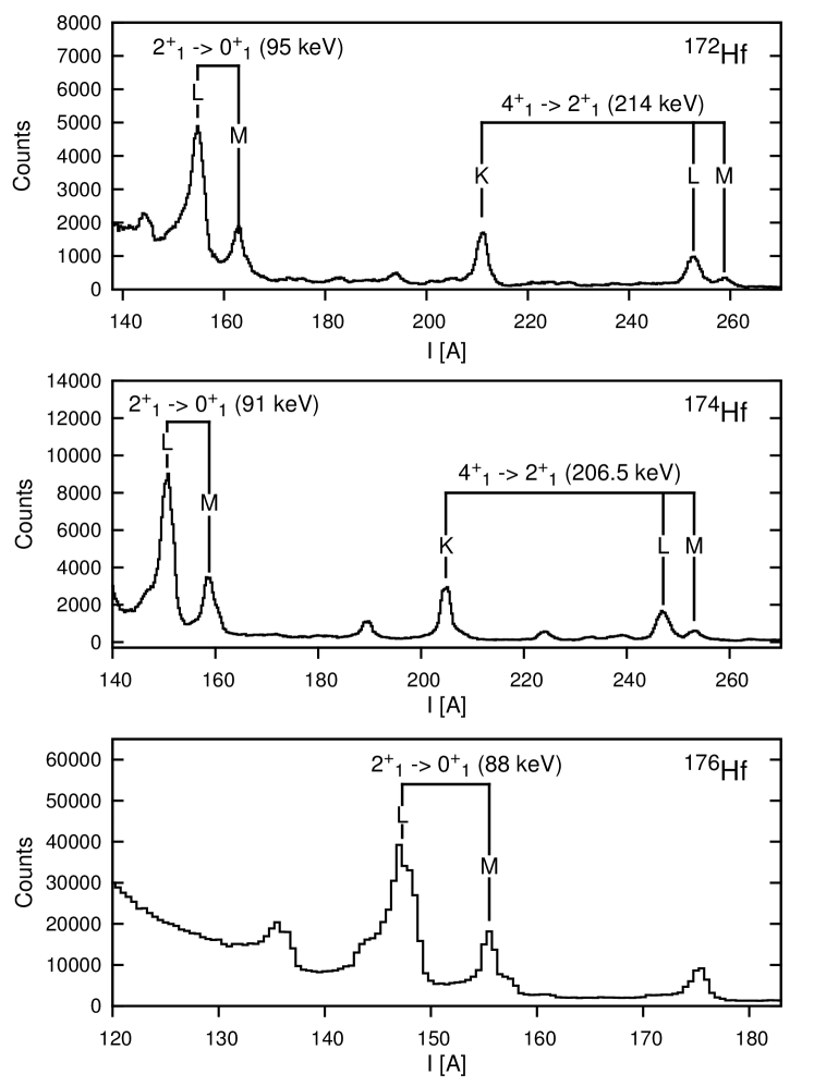
Figure 1: Conversion electron momentum spectra of the three investigated nuclei ($I$ is the current applied to the magnetic spectrometer, see text for more details). Different conversion lines from the same nuclear transition are marked accordingly. The step intervals during the scans were 0.3 A (¹⁷²Hf and ¹⁷⁴Hf) and 0.5 A (¹⁷⁶Hf).

The $\gamma$-rays were measured using a small array of six LaBr₃(Ce) (hereafter called LaBr) scintillator detectors and one high purity germanium detector (HPGe) (see Fig. 2) which were mounted perpendicular to the beam next to the target position of the Orange spectrometer. The LaBr-crystals were cylindrical and 1.5” $\times$ 1.5” in size. Four of the LaBr detectors were equipped with bismuth germanate (BGO) Compton shields and conical lead collimators to provide active Compton suppression and passive shielding. The reduction of Compton events generated in the LaBr crystal and the active suppression of stray $\gamma$ rays produced by primary Compton scattering in the experimental surrounding is important in delayed coincidence timing measurements. Such background events, including inter-detector Compton scattering (cross-talk events), are time correlated and the determination of their timing contribution poses a major source of uncertainty of the final result. The two remaining LaBr detectors were unshielded. The HPGe detector was installed perpendicular to the beam axis. Its main purpose during the experiment was to monitor the reaction, taking advantage of its energy resolution, which is superior to that of the LaBr detectors (see Figure 3(a)). In the analysis the HPGe data was used to confirm the level schemes and to identify contaminations which could otherwise possibly be overlooked in the LaBr spectra. This was especially important for the ¹⁷²Hf data, as ¹⁷²Hf is $\beta$ unstable, albeit with a long half-life of 1.87 years Gongqing (1987).

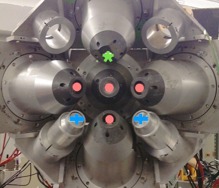
Figure 2: (Color online) Photograph of the $\gamma$ detector array in maintenance position. The position of the four BGO shielded LaBr detectors (red circles) and the two unshielded LaBr detectors (blue crosses) can be seen. Only the BGO shield is mounted where the germanium detector was positioned during the experiment (green star). The view is from the target position, the beam direction is from right to left.

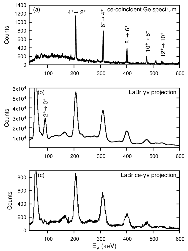
Figure 3: $\gamma$-ray spectra of ¹⁷⁴Hf from one experimental run with different coincidence conditions. (a) A spectrum measured with the Ge detector in coincidence with electrons corresponding to the L-conversion of the 2${}^{+}_{1}$ $\rightarrow$ 0${}^{+}_{1}$ transition. The Ge detector was shielded with lead and copper to suppress X rays. (b) LaBr $\gamma$-$\gamma$ projection without electron coincidence condition. (c) LaBr $\gamma$-$\gamma$ projection with the same electron coincidence condition as in (a).

Lifetimes were deduced with the method of delayed coincidences. The time difference between two signals was measured using time to amplitude converters (TACs) arranged in a fast timing circuit as described in Régis et al. (2013). The data were recorded triggerless in a list mode format and analyzed offline. This way it was possible to sort the data with a double (ce$\gamma$ and $\gamma\gamma$) as well as with a triple coincidence condition (ce$\gamma\gamma$). LaBr $\gamma\gamma$ projection spectra for both cases are shown in Fig. 3(b,c).

II.1 Half-life of $2^{+}_{1}$ states

The half-life of the 2${}^{+}_{1}$ state of ¹⁷²Hf and ¹⁷⁴Hf was determined using ce-$\gamma$ coincidences. For this purpose the Orange spectrometer was set to the electric current corresponding to the L-conversion line of the 2${}^{+}_{1}$ $\rightarrow$ 0${}^{+}_{1}$ transition. The L-conversion line was preferred over the K-conversion line because the latter lies at 23 keV, where it is buried in the $\delta$-electron background, which increases exponentially towards lower energies. Furthermore, the K-conversion coefficient $\alpha_{\mathrm{K}}$ is smaller than $\alpha_{\mathrm{L}}$ for the 2${}^{+}_{1}$ $\rightarrow$ 0${}^{+}_{1}$ transition in the investigated nuclei. E.g. $\alpha$ = 5.77, $\alpha_{\mathrm{K}}$ = 1.18, $\alpha_{\mathrm{L}}$ = 3.49 for an 88.35 keV E2 transition in ¹⁷⁶Hf. A LaBr energy gate was then set on the 4${}^{+}_{1}$ $\rightarrow$ 2${}^{+}_{1}$ transition to produce the TAC spectra shown in Figure 4 (a,b). Only the Compton suppressed LaBr detectors were used. A fit of the slope yields the half life of the first excited 2⁺ state. Several different parameterizations of the random background were tried. All variations were consistent within the uncertainty. The results are shown in Table LABEL:tab:results_172Hf - LABEL:tab:results_176Hf.

In the ¹⁷⁶Hf experiment we encountered a problem with the TAC that was started by the electron detector which was not noticed until after the beam time. It was not possible to extract reliable ce-$\gamma$ time spectra and the $\gamma$-$\gamma$ approach was therefore used in this case. The $2^{+}_{1}\rightarrow 0^{+}_{1}$ transition is highly converted and at very low energy and the $\gamma$ line in the LaBr spectra is therefore weak and on top of a lot of time-correlated background. The background subtraction, which yields the spectrum shown in Figure 4 (c), increases the uncertainty dramatically. The result agrees well with the value from Coulomb excitation measurements given in the nuclear data sheets Basunia (2006).

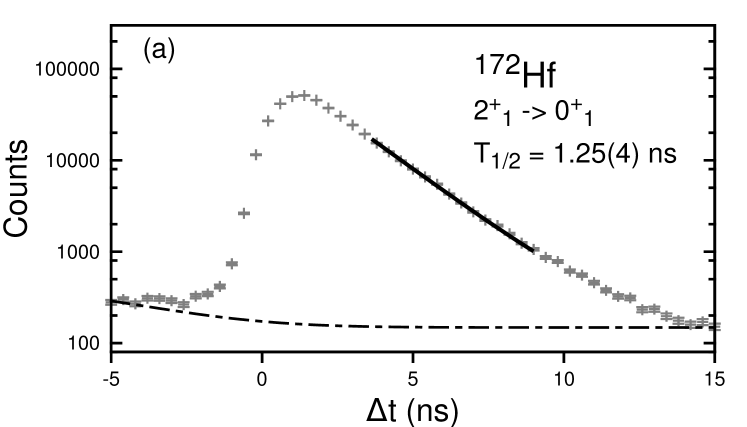
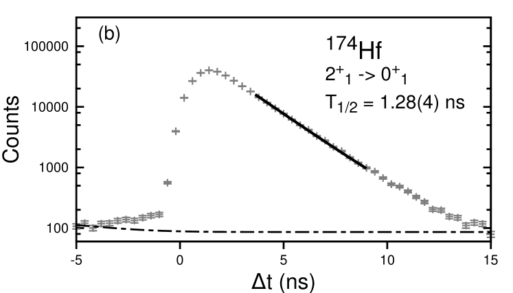
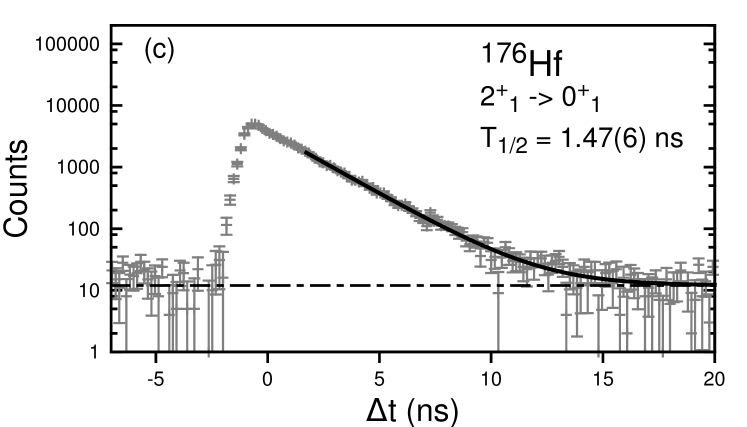
Figure 4: ce-$\gamma$ (a,b) and $\gamma$-$\gamma$ (c) delayed coincidence time spectra of the cascade $4^{+}_{1}\rightarrow 2^{+}_{1}\rightarrow 0^{+}_{1}$. Compton background has been subtracted to yield spectrum (c). The half-life was determined by fitting the slope. The best fit of an exponential function is shown as a solid line. The random background, shown as a dashed line, was determined separately.

II.2 Half-life of higher lying yrast states

For the measurement of the, previously unknown, shorter half-lives of the 4⁺, 6⁺, and 8⁺ states, TAC spectra of $\gamma$-$\gamma$ coincidences between two LaBr detectors were analyzed. LaBr coincidence energy spectra are shown in Figure 5. For these fast timing measurements in the ps region the generalized centroid difference (GCD) method was employed Régis et al. (2013), a refinement of the centroid shift method Bay (1950). With the GCD method, the centroids of two time distributions are measured for a combination of transitions that mark the population (feeding transition) and the depopulation (decay transition) of a nuclear excited state. In the case of the present setup, if the half life of the excited state is shorter than 1ps, the decay can be considered prompt. If the life time is longer a shift of the centroid is observed. If the decay is gated on the stop (stop signal on the TAC), the result is a delayed time spectrum with a centroid $C_{\mathrm{delayed}}$ shifted to the right with respect to the prompt distribution. If the decay is gated on the start (start signal on the TAC), the result is an antidelayed time spectrum with centroid $C_{\mathrm{antidelayed}}$. A lifetime will show itself as a shift of $C_{\mathrm{antidelayed}}$ to the left with respect to the prompt position. The halflife of the excited state can be measured by measuring the difference between the delayed and antidelayed centroid if the centroid difference of two prompt signals for the respective energy combination of decay and feeder is known. The necessary calibration of the prompt response difference (PRD) was obtained from measurements with a ¹⁵²Eu source, as described in detail in Régis et al. (2013), using the calibration function given in the same reference. Figure 6 shows the PRD calibration points and the fitted function for the reference energy 344 keV for the two parts of the experiment. An accuracy of $\pm$ 10 ps was adopted. Given good statistics and peak-to-background ratio, this is the main contribution to the experimental uncertainty. The experimental observable to be measured is the centroid difference $\Delta C=C_{\mathrm{delayed}}-C_{\mathrm{antidelayed}}$ which is determined from the delayed and antidelayed time spectra like the ones shown in Figure 7. The difference between $\Delta C$ and the mean PRD, shifted to a given reference energy, corresponds to twice the lifetime $\tau=\frac{T_{1/2}}{\ln(2)}$.

$$2\tau =\lvert\Delta C-\mathrm{PRD}(\Delta E_{\gamma})\rvert$$ (1)

$$\mathrm{PRD}(\Delta E_{\gamma}) =\mathrm{PRD}(E_{\mathrm{feeder}}-E_{\mathrm{decay}})$$ (2)

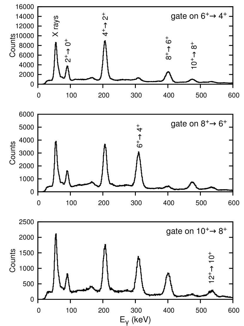
Figure 5: Examples of gated LaBr $\gamma\gamma$ coincidence spectra for ¹⁷⁴Hf. The transition which was gated on is indicated in the top-right corner of each panel. No coincident electron was demanded.

Analyzed time spectra which are measured using $\gamma$ detectors, like the ones shown in Figure 7, necessarily contain background from Compton scattering and crosstalk events. These are correlated in time with the transitions gated on, but not in the same way as the full energy peaks. This timing background is delayed with respect to the prompt response for full energy events which leads to a systematic error in $\Delta C$. Therefore a time correction related to the Compton background contribution was performed in all cases, according to the procedure outlined in reference Régis et al. (2014). The centroid of the background distribution at the gate position was determined by interpolation. By assuming that the measured distribution is the sum of the background distribution and the desired full energy response, the centroid of the latter can be determined with the additional knowledge of the peak-to-background ratio (ptb). The correction of course contributes to the measurement uncertainty $\sigma_{T_{1/2}}$. That is

$$\sigma_{T_{1/2}}=\sqrt{\sigma_{\Delta C}^{2}+\sigma_{\mathrm{PRD}}^{2}+\left[\frac{\sigma(\Delta C-\Delta C_{\mathrm{C.}})}{\mathrm{ptb}}\right]^{2}}\cdot\frac{\ln(2)}{2}$$ (3)

with $\sigma_{\Delta C}$ from the measurement of the centroid difference, and $\sigma_{\mathrm{PRD}}=10\mathrm{ps}$ from the PRD calibration, and the uncertainty from the background correction, which includes the interpolated centroid difference of the Compton background $\Delta C_{\mathrm{C.}}$. The uncertainties are those for the actually measured quantity $2\tau$. The result is then scaled to the half-life value via the rightmost factor in Eq. 3. Dependent on the ptb and the time shift between the measured CD and the interpolated time response of the Compton background $\Delta C_{\mathrm{C.}}$, the correction can be important. For an estimation of the magnitude of the correction and its effect on the uncertainty of the final half life we give an example in numbers: In the case of the 311-401 coincidence in ¹⁷⁴Hf $\mathrm{ptb-ratio}\approx 5$. The absolute value of the correction of $\Delta C$ is 2 ps, i.e. rather small. The uncertainty of $\mathrm{T}_{1/2}$ is $\sigma_{\mathrm{T}_{1/2}}=3.9\mathrm{ps}$ without background correction and $\sigma_{\mathrm{T}_{1/2,\mathrm{bg}}}=4.8\mathrm{ps}$ with background correction. In the case of the 311-417 keV coincidence in ¹⁷⁴Hf, with $\mathrm{ptb-ratio}\approx 2$, the absolute value of the correction of $\Delta C$ is about 16 ps. The uncertainties are $\sigma_{\mathrm{T}_{1/2}}=4.0\mathrm{ps}$ and $\sigma_{\mathrm{T}_{1/2,\mathrm{bg}}}=5.9\mathrm{ps}$. From this example it can be seen, that the background correction is very important, especially in the second case. The effect on the uncertainty of the final half life, however, is small compared to the contribution of the overall PRD uncertainty of 10 ps.

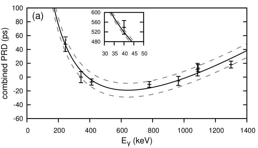
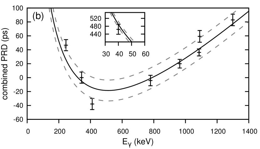
Figure 6: PRD calibration points measured with a ¹⁵²Eu source for ¹⁷²Hf, ¹⁷⁴Hf (a), and ¹⁷⁶Hf (b). The reference energy is $E_{\gamma}=344$ keV. The fitted calibration function is shown as a solid line. The uncertainty of $\pm 10$ ps is indicated as shifted dashed lines. For better comparison the data point at $E_{\gamma}=40$ keV is shown as an inlay. See text for more details.

It was possible to set a coincidence condition on the detection of a 2${}^{+}_{1}$ $\rightarrow$ 0${}^{+}_{1}$ electron for the $\gamma$-$\gamma$ timing analysis to clean the LaBr spectra. This improved the peak-to-background ratio in the LaBr energy gates used for the GCD analysis by a factor of up to 1.4 in the energy region below 300 keV. An example is shown in Figure 3. The statistics are of course drastically reduced. In the case of the strong $4^{+}\rightarrow 2^{+}$-transition, however, the systematic uncertainty due to the background is the most severe among all transitions. Therefore this approach was only used for the determination of the $4^{+}_{1}$ half-life. Throughout the analysis only time spectra from coincidences between shielded LaBr detectors were used, except in the determination of the lower half-life limit of the $8^{+}_{1}$ states. Here the transition energies are greater than $400$ keV, i.e. above the region where crosstalk events play a significant role Régis (2011). The measurement of the centroid of a single distribution imposed an uncertainty between $\pm$ 0.5 ps and $\pm$ 4 ps, depending on available statistics. Time spectra of direct feeder-decay cascades for the $4^{+}_{1}$, $6^{+}_{1}$, and $8^{+}_{1}$ states are shown in Figure 7. The spectra were re-binned to 8 ps per channel for the purpose of display. The original resolution was 2 ps per channel. All measured half-lives are summarized in the Tables LABEL:tab:results_172Hf - LABEL:tab:results_176Hf.

One merit of the GCD, which it inherits from the centroid shift method Bay (1950); Mach et al. (1989), is, that lifetimes $\tau_{1},\tau_{2},\dots$ of intermediate levels connected by a cascade of several transitions lead to a centroid shift about an effective lifetime $\tau^{\prime}$ which corresponds to the sum of the single lifetimes Mach et al. (1989)

$$\tau^{\prime}=\tau_{1}+\tau_{2}+\cdots.$$

This way it is possible to check the measured half-lives, and not least the PRD calibration, for consistency by analyzing time spectra with several coincidence conditions, i.e decay-feeder combinations. Where possible this approach was also used (see Tab. LABEL:tab:results_172Hf - LABEL:tab:results_176Hf).

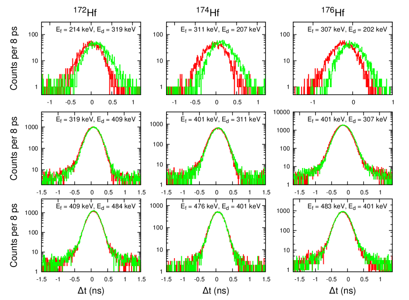
Figure 7: (Color online) $\gamma$-$\gamma$ time difference spectra for direct decay-feeder cascades in the nuclei ¹⁷²Hf (left), ¹⁷⁴Hf (center), and ¹⁷⁶Hf (right). The delayed spectra, with the decay gated on the stop branch, are shown in gray (color: green). The antidelayed spectra, where the decay is gated on the start branch, are shown in black (color: red). The top row shows the time spectra for the $6^{+}_{1}\rightarrow 4^{+}_{1}\rightarrow 2^{+}_{1}$ cascade (with ce gate), the center row those for the $8^{+}_{1}\rightarrow 6^{+}_{1}\rightarrow 4^{+}_{1}$ cascade, and the bottom those for the $10^{+}_{1}\rightarrow 8^{+}_{1}\rightarrow 6^{+}_{1}$ cascade (both without ce coincidence condition).

III Experimental results

All measured half-lives are shown in Tables LABEL:tab:BE2s along with B(E2) values. Conversion coefficients for the determination of B(E2) values were calculated using BrIccFO Kibédi et al. (2008), see Tab. LABEL:tab:ICCs.

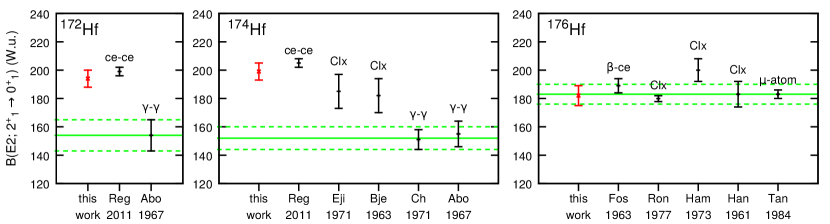
Figure 8: (Color online) Comparison of measured $B(E2,2^{+}_{1}\rightarrow 0^{+}_{1})$ values of ¹⁷²Hf, ¹⁷⁴Hf, and ¹⁷⁶Hf. The respective adopted values found in the nuclear data sheets Gongqing (1987); Browne and Junde (1999); Basunia (2006) are shown as a solid line with dashed lines indicating the uncertainty. Other data are from Han1961 Hansen et al. (1961), Bje1963 Bjerrefard et al. (1963), Fos 1963 Fossan and Herskind (1963), Abo1967 Abou-Leila (1967), Cha1971 Cha (1971), Eji1971 Ejiri and Hagemann (1971), Ron1977 Ronningen et al. (1977), Ham1973 Hammer et al. (1973), Tan1984 Tanaka et al. (1984), and Reg2011 Régis (2011). The experimental method is indicated by ce-ce, $\gamma$-$\gamma$, $\beta$-ce (delayed ce-ce, $\gamma$-$\gamma$ and $\beta$-ce coincidence fast timing), Clx (Coulomb excitation), and $\mu$-atom (muonic atom spectroscopy).

Table 1: Measured half-lives in ¹⁷²Hf. If there is more than one intermediate level, and where the final result is an upper limit, the effective half-life is given in the column T’_1/2. The adopted half-life values are set in bold face. The values determined with the GCD method are corrected for background contributions. For more details see text.

	Edecay	Efeeder	T’1/2	$\mathrm{T}_{1/2}$
state	(keV)	(keV)	(ps)	(ps)
2${}^{+}_{1}$	95	214		1250(40)
4${}^{+}_{1}$	214	319		66(5)
	214	409	78(6)	63(12)
	214	484	88(13)	70(17)
	214	543	95(18)	73(20)
6${}^{+}_{1}$	319	409		15(8)
	319	484	18(9)	15(12)
8${}^{+}_{1}$	409	484	3(7)	$<10$

Table 2: Same as in Table LABEL:tab:results_172Hf but for ¹⁷⁴Hf.

	Edecay	Efeeder	T’1/2	$\mathrm{T}_{1/2}$
state	(keV)	(keV)	(ps)	(ps)
2${}^{+}_{1}$	91			1280(40)
4${}^{+}_{1}$	207	311		77(5)
	207	401	101(6)	85(9)
	207	476	99(15)	84(15)
	207	941	65(47)	49(52)
	207	1252		72(47)
6${}^{+}_{1}$	311	401		16(5)
	311	476	22(6)	18(8)
8${}^{+}_{1}$	401	476	5(5)	$<10$

Table 3: Same as in Table LABEL:tab:results_172Hf but for ¹⁷⁶Hf.

	Edecay	Efeeder	T’1/2	$\mathrm{T}_{1/2}$
state	(keV)	(keV)	(ps)	(ps)
2${}^{+}_{1}$	88	202		1470(60)
4${}^{+}_{1}$	202	307		90(6)
	202	401	110(6)	93(9)
	202	483	114(6)	92(12)
	202	736	109(8)	93(11)
	202	1043		97(13)
6${}^{+}_{1}$	307	401		17(6)
	307	483	23(7)	18(11)
8${}^{+}_{1}$	401	483	6(9)	$<15$

Table 4: Adopted values of the measured half-lives (see Tables LABEL:tab:results_172Hf-LABEL:tab:results_176Hf) and the corresponding B(E2) value for the transition to the next lower lying state in the ground state rotational band.

	172Hf		174Hf		176Hf
	T1/2	B(E2)	T1/2	B(E2)	T1/2	B(E2)
state	(ps)	(W.u.)	(ps)	(W.u.)	(ps)	(W.u.)
2${}^{+}_{1}$	1250(40)	194(6)	1280(40)	199(6)	1470(60)	182(7)
4${}^{+}_{1}$	66(5)	274(18)	77(5)	270(20)	90(6)	251(18)
6${}^{+}_{1}$	15(8)	$177(^{+81}_{-42})$	16(5)	$197(^{+90}_{-47})$	17(6)	$195(^{+106}_{-51})$
8${}^{+}_{1}$	$<$10	$>$85	$<$10	$>$91	$<$15	$>$60

Figure 8 shows a comparison of the results from this work with results from earlier measurements of $B(E2,2^{+}_{1}\rightarrow 0^{+}_{1})$ in the three hafnium isotopes which were investigated. For ¹⁷²Hf there is one other measurement which also applied the $\gamma\gamma$ fast timing method, by Abou-Leila Abou-Leila (1967) who gives a value of $T_{1/2}=1.55(10)$ ns. This results in $B(E2,2^{+}_{1}\rightarrow 0^{+}_{1})=154(11)$ W.u., which is several $\sigma$s lower than the value from this work. Another measurement, performed using ce-ce fast timing with the Cologne Double Orange Spectrometer, resulted in $B(E2,2^{+}_{1}\rightarrow 0^{+}_{1})=199(3)$ W.u. Régis (2011), in agreement with the value found in this work. The situation is similar for ¹⁷⁴Hf, for which the Nuclear Data Base gives an adopted value of $B(E2,2^{+}_{1}\rightarrow 0^{+}_{1})=152(8)$ W.u. Browne and Junde (1999). Two sources are cited which also used $\gamma$-$\gamma$ fast timing. From those the adopted value is calculated. One measurement, however, used Coulomb excitation Ejiri and Hagemann (1971), yielding a significantly larger value of $B(E2,2^{+}_{1}\rightarrow 0^{+}_{1})=184(13)$ W.u. This is in agreement with the value determined in this work. A ce-ce fast timing measurement resulted in $B(E2,2^{+}_{1}\rightarrow 0^{+}_{1})=201(3)$ W.u., also much higher than the value adopted by the Nuclear Data Sheets. For ¹⁷⁶Hf the value of this work agrees well with the one adopted by the NNDC. In this case the sources do not contain any $\gamma$-$\gamma$ fast timing experiments from before 1972. The measurements which resulted in the low values cited above were all performed in the late 1960s, and used NaI detectors. The energy resolution of these detectors is much worse than that of LaBr detectors used today. Under such circumstances it is difficult to control and estimate the background contributions, especially for transitions as low in energy as the $2^{+}_{1}\rightarrow 0^{+}_{1}$ transition in deformed nuclei, which typically lie around or below 100 keV. For this reason we will adopt the $B(E2,2^{+}_{1}\rightarrow 0^{+}_{1})$ values measured in this work for our further discussion. The other half-lives and absolute transition strengths measured in this work are measured for the first time.

Table 5: Internal conversion coefficients (ICCs) from BrIccFO Kibédi et al. (2008) used for the calculation of B(E2) values.

	internal conversion coefficient $\alpha$
transition	172Hf	174Hf	176Hf
$2^{+}_{1}\rightarrow 0^{+}_{1}$	4.32(6)	5.12(8)	5.86(9)
$4^{+}_{1}\rightarrow 2^{+}_{1}$	0.230(4)	0.256(4)	0.278(4)
$6^{+}_{1}\rightarrow 4^{+}_{1}$	0.0660(10)	0.0711(10)	0.0739(11)
$8^{+}_{1}\rightarrow 6^{+}_{1}$	0.0327(5)	0.0345(5)	0.0345(5)

The new $B(E2)$ values complete the picture of evolution of quadrupole transition strength in the ground state band of mid-shell hafnium isotopes. The result is a smooth increase from low neutron numbers $N$ towards mid-shell and a subsequent smooth decrease (see Fig. 9 (a)). It is well established that the investigated hafnium isotopes display the characteristics of an axially deformed rotor. In such nuclei the ratio $B_{42}=B(E2,4^{+}_{1}\rightarrow 2^{+}_{1})/B(E2,2^{+}_{1}\rightarrow 0^{+}_{1})$ can be calculated as the ratio of Clebsch-Gordan coefficients (Alaga rules), which yields $B_{42}=1.43$. As can be seen in Figure 9 (b), the newly measured transition strengths fit well into the systematics for rigid rotors, as expected.

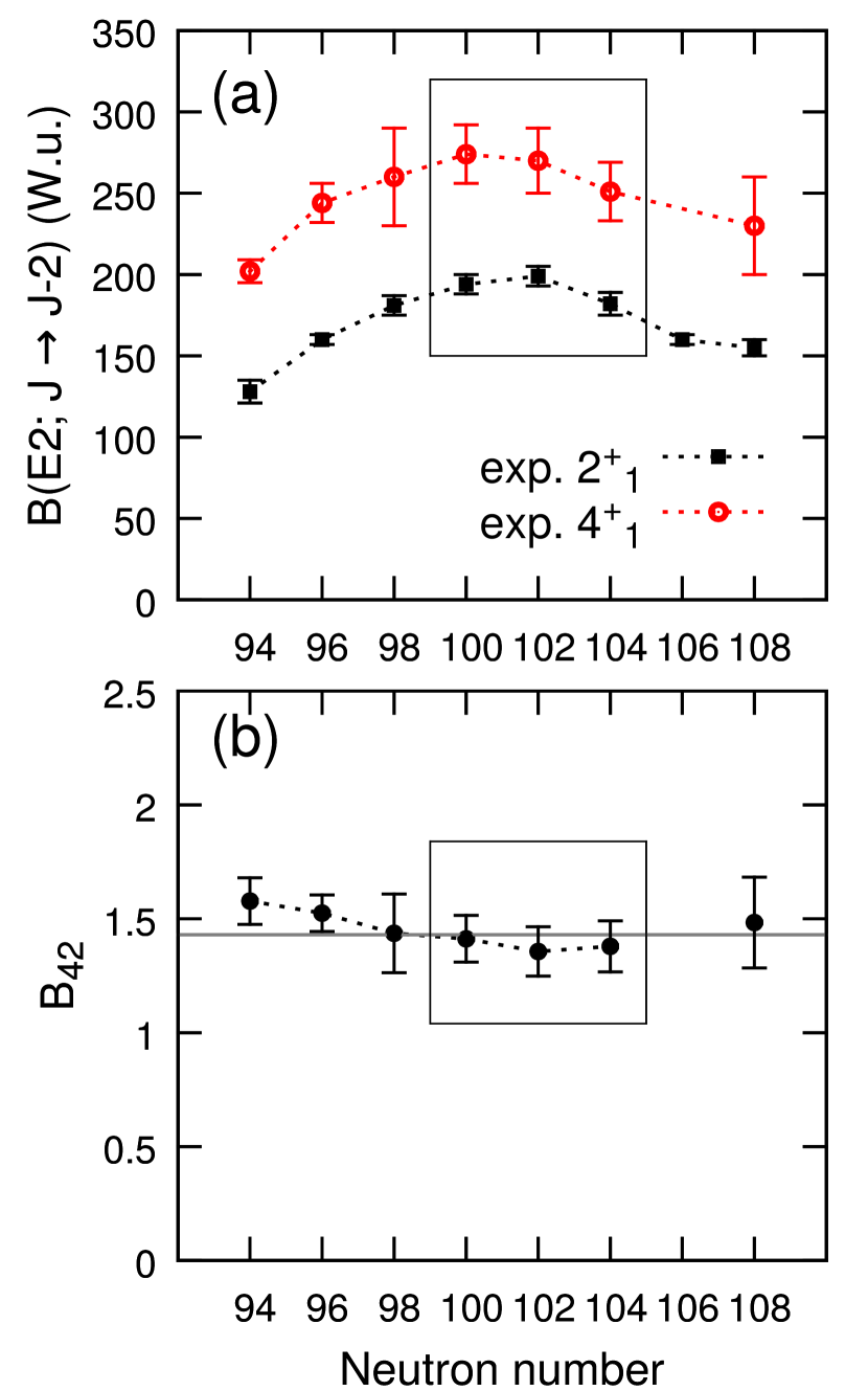
Figure 9: (Color online) Experimental $B(E2;J\rightarrow J-2)$ values in hafnium isotopes (Z=72) (a) and the ratio $B_{42}=B(E2,4^{+}_{1}\rightarrow 2^{+}_{1})/B(E2,2^{+}_{1}\rightarrow 0^{+}_{1})$ (b). Values measured in this work are marked with a box. Other values are taken from the Nuclear Data Sheets Baglin (2008, 2010, 2002); Achterberg et al. (2009); WU and NIU (2003).

IV Calculation and discussion

IV.1 Description of the model and discussion of mean-field results

To help understand the data, we have performed theoretical calculations of spectroscopic properties by employing the recently proposed methodology of Refs. Nomura et al. (2008, 2011b). The essential idea of the method is to determine the Hamiltonian of an appropriate version of the IBM by computing the bosonic deformation energy surface so that it reproduces, in a way described below, the basic topology of the deformation energy surface of the many-fermion system computed microscopically with the HFB method. The resultant Hamiltonian is used to calculate energy levels and wave functions of excited states.

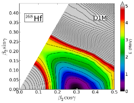
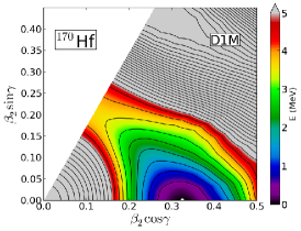
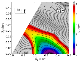
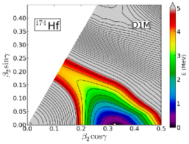
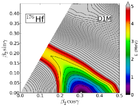
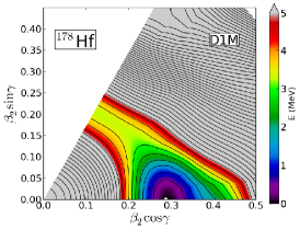
Figure 10: (Color online) Contour plots of the deformation energy surfaces in terms of the quadrupole deformations $\beta_{2}$ and $\gamma$ for the nuclei ^168-178Hf, obtained from the Gogny HFB calculations using the D1M interaction. The color scale varies in steps of 0.25 MeV and the contour lines are drawn in steps of 0.5 MeV. The range of the plot is $0.0\leqslant\beta\leqslant 0.5$ and $0^{\circ}\leqslant\gamma\leqslant 60^{\circ}$. The absolute minimum is identified by an open circle.

Our starting point is the microscopic calculation of the deformation energy surface within the self-consistent mean-field model. We have performed, for each individual Hf nucleus, a set of the constrained Hartree-Fock-Bogoliubov (HFB) calculations, and obtained the deformation energy surfaces in terms of the quadrupole collective coordinates $\beta$ and $\gamma$ Bohr and Mottelsson (1975). It is also possible to parametrize the energy surfaces using the quadrupole moments $Q_{20}$ and $Q_{22}$ related to the $\beta$ and the $\gamma$ variables by $\beta=\sqrt{\frac{4\pi}{5}}\frac{Q}{A\langle r^{2}\rangle}$ and $\gamma=\tan^{-1}\frac{Q_{22}}{Q_{20}}$ with $Q=\sqrt{Q_{20}^{2}+Q_{22}^{2}}$ (see Ref. Nomura et al. (2011b) for more details). In the definition of $\beta$ we use the mean-squared radius $\langle r^{2}\rangle$ evaluated with the corresponding HFB state. Throughout this work, the D1M parametrization of the Gogny energy density functional Goriely et al. (2009) is employed for the effective nucleon-nucleon interaction.

In Fig. 10, the deformation energy surfaces obtained from the Gogny-D1M HFB calculations for the ^168-180Hf nuclei, are plotted in terms of the $\beta$ and $\gamma$ deformations. We limit the plot to the range $0.0\leqslant\beta\leqslant 0.5$ and $0^{\circ}\leqslant\gamma\leqslant 60^{\circ}$, because it is the relevant scope for our purposes. Energy surfaces for ¹⁶⁶Hf and ¹⁸⁰Hf are not shown because they are quite similar in topology to the ones of the adjacent nuclei ¹⁶⁸Hf and ¹⁷⁸Hf, respectively. In general, the energy minimum is located around $\beta=0.3$ on the $\gamma=0$ axis, being characteristic of an axially deformed prolate rotor. While any significant change in the topology is visible from the microscopic energy surface, the minimum appears to be steeper in both $\beta$ and $\gamma$ directions for heavier Hf isotopes. Although not shown here, the results with D1S look quite similar to the D1M ones. However, as compared to the D1M results, the energy minima of the D1S energy surfaces are steeper both in $\beta$ and $\gamma$ directions than in the D1M case. In Table LABEL:tab:pes we observe that for the nuclei ^170-178Hf the HFB energy of the minimum (relative to the energy of the spherical configuration ($\beta,\gamma$)=(0,0) and denoted as $E_{min}$) is generally around 1.2-1.7 MeV smaller in magnitude in the D1M case than the D1S one.

Table 6: The HFB energy at the minimum (relative to the spherical configuration, and denoted by $E_{min}$) as well as the position of the minimum $\beta_{2,min}$ are given for both parametrizations of the Gogny force and the ^170-178Hf nuclei.

	$E_{min}$ (MeV)		$\beta_{2,min}$
	D1S	D1M	D1S	D1M
170Hf	-12.214	-10.944	0.339	0.325
172Hf	-13.788	-12.277	0.360	0.332
174Hf	-14.724	-13.061	0.353	0.326
176Hf	-15.068	-13.385	0.320	0.307
178Hf	-14.960	-13.328	0.301	0.288

In Fig. 11 the $\beta$ value at the absolute minimum of the microscopic energy surface (denoted hereafter as $\beta_{2,min}$) is plotted as a function of neutron number. It exhibits a parabolic behavior with its maximum at $N=100$ instead of the mid-shell value $N=104$. The D1S results are generally larger than the D1M ones but in both cases they show their maximum value at $N=100$. However, as observed in Table LABEL:tab:pes, the minimum energy $E_{min}$ reaches its maximum at mid-shell for both the D1S and the D1M sets.

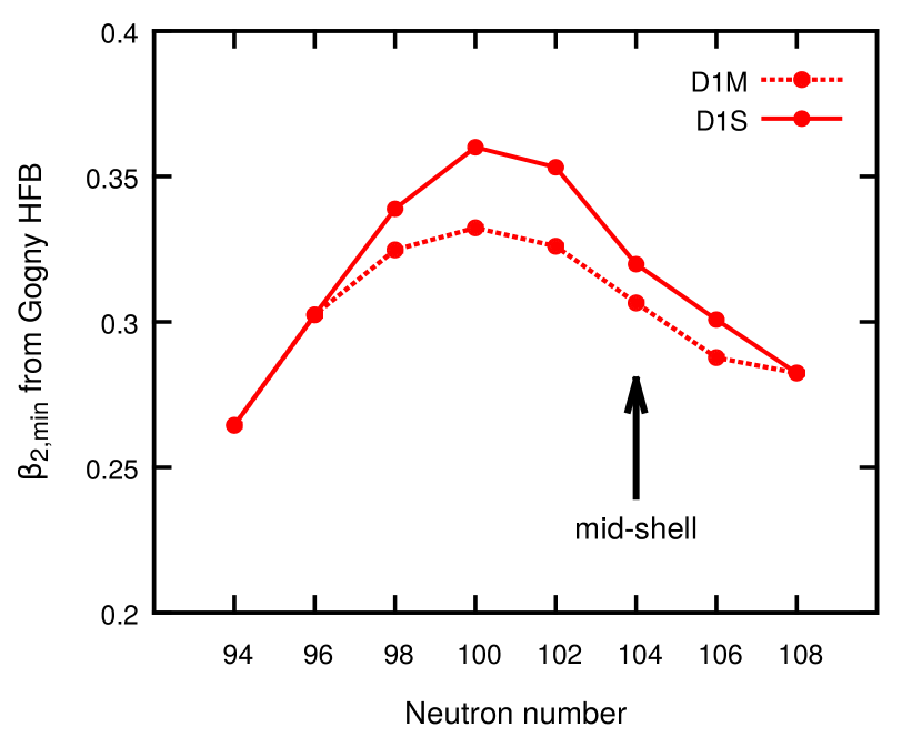
Figure 11: (Color online) The $\beta_{2,min}$ values, where the HFB energy has its absolute minimum are plotted as a function of neutron number for the ^166-180Hf isotopes. Solid and dotted curves represent the results from D1S and D1M interactions, respectively.

For the boson calculation, we employ the following proton-neutron IBM (IBM-2) Hamiltonian:

$$\hat{H}_{\textnormal{IBM}}=\epsilon(\hat{n}_{d\pi}+\hat{n}_{d\nu})+\kappa\hat{Q}_{\pi}\cdot\hat{Q}_{\nu}+\kappa^{\prime}\hat{L}\cdot\hat{L},$$ (4)

where the first and the second terms stand for the $d$-boson number operator and the quadrupole-quadrupole interactions, respectively. They are given by the expressions $\hat{n}_{d\tau}=d^{\dagger}_{\tau}\cdot\tilde{d}_{\tau}$ and $\hat{Q}_{\tau}=s^{\dagger}_{\tau}\tilde{d}_{\tau}+d^{\dagger}_{\tau}s^{\dagger}_{\tau}+\chi_{\tau}[d^{\dagger}_{\tau}\times\tilde{d}_{\tau}]^{(2)}$ with $\tau$ being either $\pi$ (proton) or $\nu$ (neutron). The third term is relevant for rotational bands and it is shown Nomura et al. (2011b) to be necessary for the description of deformed nuclei. It is given in terms of the total angular momentum operator $\hat{L}=\hat{L}_{\pi}+\hat{L}_{\nu}$ with $\hat{L}_{\tau}=\sqrt{10}[d^{\dagger}_{\tau}\times\tilde{d}_{\tau}]^{(1)}$.

The most general IBM-2 Hamiltonian contains many more terms and parameters than the one in Eq. (4). The present IBM-2 Hamiltonian is rather simple compared with a general Hamiltonian, but contains the minimal number of interaction terms relevant for the description of low-lying quadrupole states. The Hamiltonian parameters are determined by mapping the HFB energy surface onto the IBM one. Some technical details of the procedure are described in Appendix A. In Table 7 we tabulate the IBM-2 parameters determined by the mapping procedure for the ^166-180Hf isotopes.

Table 7: The parameters for the IBM Hamiltonian $\hat{H}_{\rm IBM}$ of Eq. (4), as well as the proportionality coefficient $C_{\beta}$ for the deformation parameter $\beta$, obtained from the mapping of the HFB to the IBM energy surfaces for ^166-180Hf.

$A$	$\epsilon$	$-\kappa$	$\chi_{\pi}$	$\chi_{\nu}$	$\kappa^{\prime}$	$C_{\beta}$	$e_{B}$
	(keV)	(keV)	$\times 10^{3}$	$\times 10^{3}$	(keV)		($e$fm2)
166	474	281	213	-813	-9.95	3.65	15.3
168	439	285	213	-729	-11.9	3.20	16.3
170	451	292	241	-895	-13.0	2.96	15.9
172	333	281	454	-878	-10.5	2.96	15.5
174	238	267	303	-768	-6.46	3.00	14.3
176	166	242	237	-723	-2.00	3.30	12.9
178	97.7	258	709	-1086	-0.952	3.50	12.3
180	88.0	273	359	-801	-3.36	3.60	13.5

Having all the relevant parameters at hand, the Hamiltonian is diagonalized to obtain energies and wave functions of the excited states. For the numerical diagonalization of the IBM-2 Hamiltonian and the calculations of the E2 transition rates, the computer program NPBOS T. Otsuka, N. Yoshida has been used. Using the resultant wave functions, the transition probabilities between the states are calculated. In particular, the $B$(E2;$J\rightarrow J^{\prime}$) value is obtained by

$$B({\textnormal{E2}};J\rightarrow J^{\prime})=\frac{1}{2J+1}|\langle J^{\prime}||\hat{T}^{(E2)}||J\rangle|^{2},$$ (5)

where $J$ and $J^{\prime}$ are the total angular momenta of the initial and the final states of the transition, respectively. The E2 operator is written as $\hat{T}^{(E2)}=e_{\pi}\hat{Q}_{\pi}+e_{\nu}\hat{Q}_{\nu}$, where $\hat{Q}_{\tau}$ is the quadrupole operator defined in Eq. (4) and the same values of $\chi_{\pi,\nu}$ parameters are used. The parameter $e_{\tau}$ is the boson effective charge for proton and neutron. Here we assume that the effective charge is the same for protons and neutrons, $e_{\pi}=e_{\nu}\equiv e_{B}$. In most of the previous IBM calculations, a fixed value of the effective charge $e_{B}$, that is determined by fitting to the experimental data for the $B$(E2) values, is used for all members of the isotopic chain.

IV.2 Energy levels

Figure 12: (Color online) Experimental (a) and the theoretical (D1M parametrization) (b) level energies of the low-lying yrast $2^{+}$, $4^{+}$, $6^{+}$, $8^{+}$ and $10^{+}$ states as functions of neutron number.

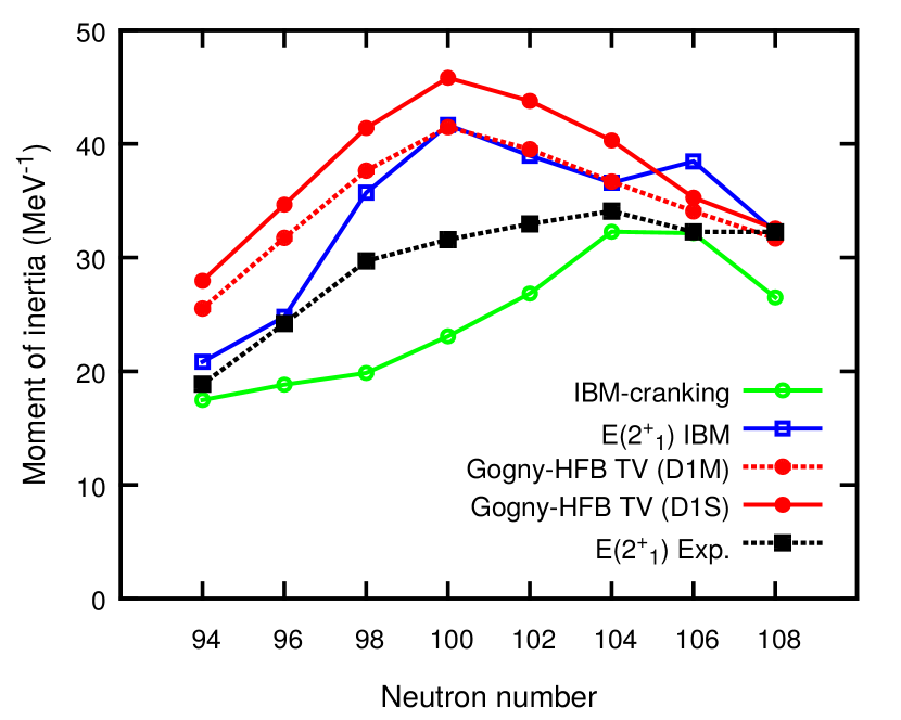
Figure 13: (Color online) The moments of inertia (MOIs) of the ground state rotational band of the ^166-180Hf nuclei obtained in different approaches are plotted as a function of neutron number. The MOIs are computed using the cranking calculations of the IBM in the coherent state “IBM-cranking” and the self-consistent HFB cranking method that leads to the Thouless-Valatin MOI both with the D1M “Gogny-HFB TV (D1M)” and the D1S “Gogny-HFB TV (D1S)” parametrizations. Also shown are the MOI extracted from the $2^{+}_{1}$ excitation energies of the IBM-2 “$E(2^{+}_{1})$ IBM” and the experiment “$E(2^{+}_{1})$ Exp.” using the rigid rotor formula.

In order to confirm that the present framework gives a reasonable description of the energy levels, we display in Fig. 12 the experimental level energies for the yrast $2^{+}$, $4^{+}$, $6^{+}$, $8^{+}$ and $10^{+}$ states and the corresponding theoretical level energies calculated by the mapped IBM-2. Overall, our IBM-2 calculation follows the experimental trend satisfactorily, and reproduces the energies for each nucleus rather well at a quantitative level. However, the energy levels have a minimum as a function of neutron number at mid-shell $N=104$ in the experiment, while the minimum is at $N=100$ in the theory.

To illustrate this deviation of the $2^{+}_{1}$ excitation energy, we show in Fig. 13 the moments of inertia (denoted as MOI) of the rotational band, obtained from the rotor formula $E(J)\propto J(J+1)$ (with $J=0^{+},2^{+},4^{+},\ldots$) and the $2^{+}$ energies of the IBM result (denoted as “$E(2^{+}_{1})$ IBM” in the figure) and the experiment (“$E(2^{+}_{1})$ Exp.”). The moment of inertia, which is equal to $3/E(2^{+}_{1})$, of the IBM is maximal at $N=100$, while the experimental MOI at $N=104$ but changes much less than the theoretical value with neutron number.

The reason for the discrepancy in the systematics of the MOI between the IBM result and the experiment can be due to the inclusion of the $\hat{L}\cdot\hat{L}$ term in the IBM-2 Hamiltonian. To shed more light upon this point, we plot in the same figure the MOI obtained from the cranking calculation in the Gogny HFB model using the Thouless-Valatin (TV) formula Thouless and Valatin (1962) (denoted as “Gogny-HFB TV” in the figure for the two different parametrizations D1S and D1M), and the one calculated in the IBM without the $\hat{L}\cdot\hat{L}$ term (denoted as “IBM-cranking”). As described in Appendix A, the coefficient of the $\hat{L}\cdot\hat{L}$ term is determined so that the “IBM-cranking” MOI becomes identical to the “Gogny-HFB TV (D1M)” one. For that reason, we do not plot the IBM cranking MOI with the $\hat{L}\cdot\hat{L}$ term. In Fig. 13, one should see that the “IBM-cranking” MOI is peaked at $N=104$ or 106, consistent with the experimental MOI while the “Gogny-HFB TV (D1M)” MOI is peaked at $N=100$ (the same applies for the D1S values). For the nuclei with $N\leq 102$, the difference between the “IBM-cranking” and the “Gogny-HFB TV (D1M)” MOIs is rather large as compared to the one for $N\geq 104$. Thus, the lowering of the energy due to the inclusion of the $\hat{L}\cdot\hat{L}$ is much more significant in the $N\leq 102$ Hf nuclei than in the $N\geq 104$ ones. Consequently, the maximum point of the “$E(2^{+}_{1})$ IBM” MOI appears at $N=100$ due to the inclusion of the $\hat{L}\cdot\hat{L}$ term. This correlates with the evolution of the derived $\kappa^{\prime}$ parameter, presented in Table 7: for example, the parameter $\kappa^{\prime}$ for ¹⁷²Hf is much larger in magnitude than that for ^176,178Hf. We also note that the same conclusion would be extracted from the D1S parametrization as it predicts the same systematics as the D1M set.

It is certainly worth noting that, contrary to the empirical trend, the Thouless-Valatin MOI becomes maximal, irrespectively of the choice of the parametrizations, not at the mid-shell $N=104$ and that this systematics is well correlated with the evolution of the $\beta_{2,min}$ in Fig. 11.

On the other hand, it has been shown Afanasjev et al. (2000) that the moment of inertia of the ground-state rotational band calculated in the cranking model is rather sensitive to the details of the pairing interaction. Therefore, it can be of interest that a small modification to the relevant channel in the D1S and D1M functionals could lead to a substantial improvement of the agreement with the experimental data.

Finally, we also note that the calculation generally underestimates the experimental level energies, in particular, for the nucleus ¹⁷²Hf. The reason would be that the effect of including the $\hat{L}\cdot\hat{L}$ term is rather significant, as the TV MOI from the Gogny-HFB calculation overestimates the experimental one considerably (see Fig. 13).

IV.3 E2 transitions

Let us now turn our attention to the calculation of the $B$(E2) values. In Fig. 14(a) the theoretical $B$(E2;$J\rightarrow J-2$) values ($J=2,4,\ldots,10$) calculated with an effective charge $e_{B}=0.123$ $e$b are shown. The effective charge was fixed for all the considered Hf nuclei as to reproduce the experimental $B({\textnormal{E2}};2^{+}_{1}\rightarrow 0^{+}_{1})$ value of 182 W.u in ¹⁷⁶Hf. As anticipated from previous IBM fitting calculations for W and Os isotopes Rudigier et al. (2010), the theoretical $B$(E2;$J\rightarrow J-2$) values with a fixed $e_{B}$ value become maximal at mid-shell $N=104$, which disagrees with the experimental $B$(E2) systematics showing a peak at $N=100$ or 102.

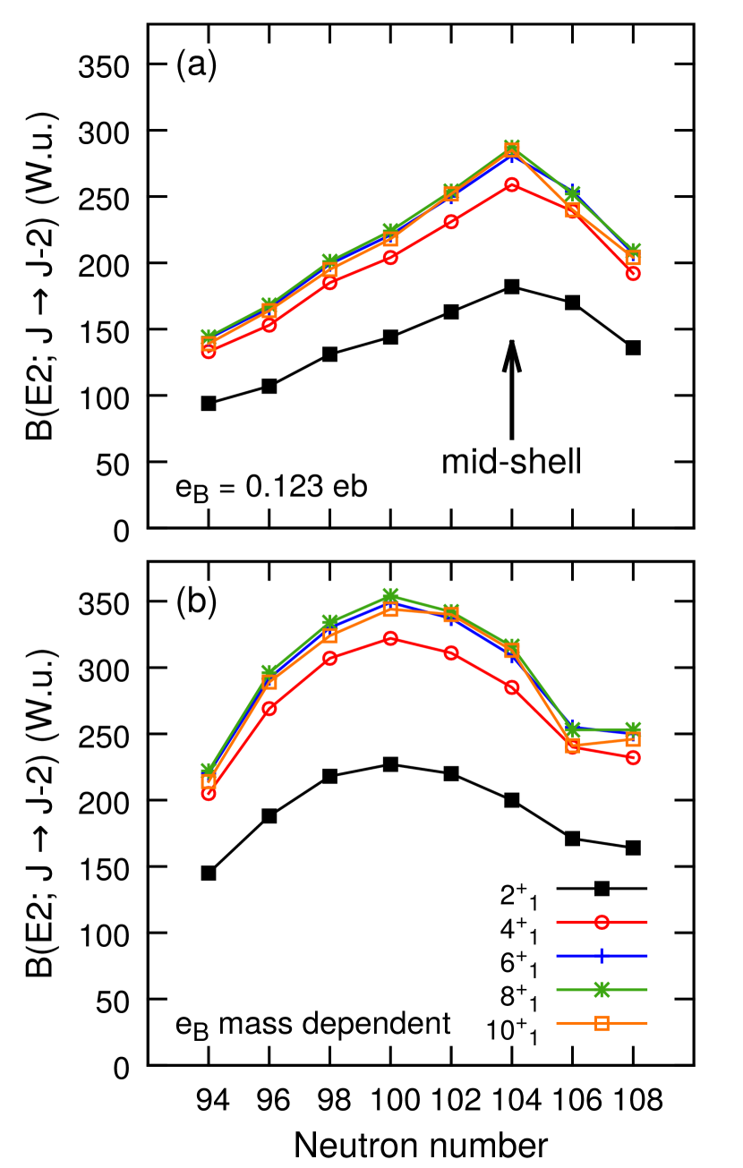
Figure 14: (Color online) The $B$(E2) values for hafnium ($Z$=72) isotopes calculated with two different choices of effective boson charge $e_{\mathrm{B}}$: (a) $e_{\mathrm{B}}=0.123\mathrm{eb}$ fixed for all isotopes; (b) $e_{B}$ different from nucleus to nucleus, each determined by adjusting the transition quadrupole moment $Q_{t}(2^{+}_{1}\rightarrow 0^{+}_{1})$ from the IBM-2 calculation to fit $\beta_{2,\mathrm{min}}$ of the Gogny-HFB D1M calculation. The boson effective charges $e_{B}$ used for the latter calculation are tabulated in Table 7.

The failure can be partly attributed to the use of a fixed effective charge $e_{\mathrm{B}}$. Then, we consider $e_{\mathrm{B}}$ to be mass dependent and determine its value for each individual nucleus. Specifically, we propose to derive $e_{\mathrm{B}}$ so that it follows the systematics of the Gogny-HFB $\beta_{2,min}$ values, mainly because this quantity reaches its maximum value not at mid-shell but at $N=100$, as seen from Fig. 11.

A possible option to take this effect into account can be to associate the transition quadrupole moment $Q_{t}$, corresponding to the $2^{+}_{1}\rightarrow 0^{+}_{1}$ E2 transition matrix element, to the Gogny-HFB $\beta_{2,min}$ value. In general, $Q_{t}$ for the transition from the state with spin $J$ to $J^{\prime}$ is written as

$$Q_{t}(J\rightarrow J^{\prime})=\sqrt{\frac{16\pi}{5}\frac{B({\textnormal{E2}};J\rightarrow J^{\prime})}{(J200|J^{\prime}0)^{2}}},$$ (6)

with $(J200|J^{\prime}0)$ being the Clebsch-Gordan coefficient. The quantity $Q_{t}(J\rightarrow J^{\prime})$ is transformed into the intrinsic deformation parameter $\beta_{t}(J\rightarrow J^{\prime})$

$$\beta_{t}(J\rightarrow J^{\prime})=\frac{\sqrt{5\pi}}{3ZR^{2}}Q_{t}(J\rightarrow J^{\prime}).$$ (7)

The $\beta_{t}$ for the $2^{+}_{1}\rightarrow 0^{+}_{1}$ E2 transition, $\beta_{t}(2^{+}_{1}\rightarrow 0^{+}_{1})$, is eventually made equal, for each individual nucleus, to the Gogny-HFB mean-field $\beta_{2,min}$ in order to obtain the effective charge $e_{\mathrm{B}}$.

In Fig. 14(b) we plot the resulting $B$(E2;$J\rightarrow J-2$) values with the effective charge determined in this way. Although the $B$(E2;$J\rightarrow J-2$) values in panel (b) are generally larger in magnitude than those in panel (a), the systematic trend is more consistent with the experimental one, as it becomes maximal at $N=100$, not at the mid-shell nucleus ¹⁷⁶Hf. Again, one notices that the result is well correlated with the Gogny-HFB $\beta_{2,min}$ value (Fig. 11), the Thouless-Valatin MOI (Fig. 13), and the variation of the extracted $e_{\mathrm{B}}$ value as a function of $N$ (Tab. 7).

The observed experimental $B$(E2) systematics in the neutron-deficient Hf isotopes, indicating the maximum collectivity not at the middle of the major shell, implies that for the analysis of realistic nuclei a simple model may not be sufficient and that certain microscopic effects have to be taken into account. In particular, the mass-dependence of $e_{\mathrm{B}}$ implies that the effect of the core polarization may become non-negligible. In the present IBM framework, the polarization effect cannot be included explicitly, but it could be somehow taken into account by absorbing it in the variation of the boson charge.

Alternatively, the mass dependence of the boson effective charge could be explained by the renormalization effect of the $g$ boson Otsuka and Ginocchio (1985). In the $sd$ IBM system, the $g$-boson effect could show up as higher-order terms in the quadrupole operator Otsuka and Ginocchio (1985). In that sense, the form of the quadrupole operator used in the present work in Eq. (4), which is a one-body operator, can be extended to include the higher-order terms.

We also comment on the dependence of the IBM results on the choice of the EDF parametrization. For the energies of the ground-state rotational band, there is a certain quantitative difference between the D1S and the D1M results, but the overall tendency at the qualitative level is expected to be quite similar, because the deformation energy surface, $\beta_{2,min}$ and Thouless-Valatin MOI for both parametrizations have been shown to exhibit similar features as a function of neutron number. Likewise, for the $B$(E2) systematics, as both the D1S and D1M sets provide a similar trend of the $\beta_{2,min}$ value (cf. Fig. 11), if the effective charges are determined in the same way, one would obtain the results qualitatively similar to the ones from the D1M interactions (cf. Figs. 14 and 15).

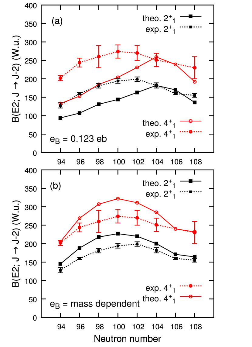
Figure 15: (Color online) Comparison of experimental and theoretical reduced transition strengths in hafnium isotopes (Z=72). (a) Calculation from Fig. 14 (a) ($e_{\mathrm{B}}=0.123\mathrm{eb}$). (b) Calculation from Fig. 14 (b) ($e_{\mathrm{B}}$ mass dependent).

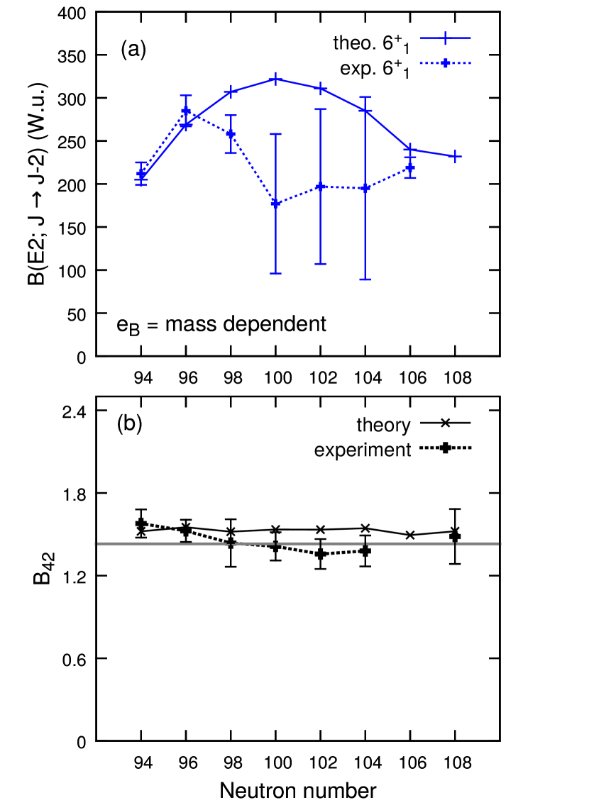
Figure 16: (Color online) Comparison of experimental and theoretical reduced transition strengths in hafnium isotopes (Z=72). (a) Calculation from Fig. 14 (b) ($e_{\mathrm{B}}$ mass dependent). (b) $B_{42}$ as defined in the text. The IBM SU(3) limit of $B_{42}=10/7$ is indicated as a gray line.

For completeness, in Fig. 15 we compare the $B$(E2;$4^{+}_{1}\rightarrow 2^{+}_{1}$) and $B$(E2;$2^{+}_{1}\rightarrow 0^{+}_{1}$) experimental values with the results of the calculations with two different choices of the effective charge: (a) $e_{\mathrm{B}}=0.123$ $e$b fixed for all nuclei, and (b) $e_{B}$ dependent on mass. In Fig. 16, we compare the experimental and theoretical (with the use of mass-dependent effective charge) $B$(E2;$6^{+}_{1}\rightarrow 4^{+}_{1}$) value (a) and the $B_{42}$ ratio (b). It is rather evident from Figs. 15(a,b) that the calculations with the fixed boson effective charge do not reproduce the experimental trend while a nice agreement between theory and calculation is obtained if one chooses the effective charge for each nucleus as to follow the variation of the $\beta_{2,min}$ value with $N$. Overall, a reasonable description of the data is obtained both qualitatively and quantitatively.

In Fig. 15(b), the calculated $B$(E2;$4^{+}_{1}\rightarrow 2^{+}_{1}$) and $B$(E2;$2^{+}_{1}\rightarrow 0^{+}_{1}$) values overestimate the experimental values for the nuclei around $N=100$. This might be due to the presence of a non-zero hexadecapole deformation $\beta_{4}$. A non-zero $\beta_{4}$ has an influence on the transition quadrupole moment $Q_{t}$, and therefore on the extracted effective charge. Likely, the inclusion of $\beta_{4}$ will improve agreement with experiment for these nuclei. In fact, the previous IBM-1 calculation indicated Zerguine et al. (2008) that the hexadecapole degree of freedom may be non-negligible, though in a different context of some ground-state properties.

For the $6^{+}_{1}\rightarrow 4^{+}_{1}$ E2 transition presented in Fig. 16(a), the theoretical value shows a parabolic behavior. The experimental one does not show this trend, but also has a large uncertainty. In Fig. 16(b), we observe that both the experimental and theoretical $B_{42}$ ratio are close to each other, as well as to the SU(3) limit of the IBM (=10/7) Arima and Iachello (1987), showing that the considered nuclei are well described as being good rotors.

In comparison to the other EDF-based calculation available in the literature, the five-dimensional collective Hamiltonian approach based on the Gogny-D1S parameter set has predicted the maximum $B$(E2;$2^{+}_{1}\rightarrow 0^{+}_{1}$) value at $102$ CEA . It is one unit different from our result, but in that calculation the difference in the $B$(E2;$2^{+}_{1}\rightarrow 0^{+}_{1}$) values between ¹⁷²Hf and ¹⁷⁴Hf is negligible.

V Conclusion

The experimental technique of fast timing using a combination of LaBr detectors and a conversion electron spectrometer, is very well suited to measure yrast B(E2) values in deformed nuclei. It was possible to measure the half-lives of ground state band excitations of a nucleus from the $2^{+}_{1}$ to the $6^{+}_{1}$ state in one single experiment with a relatively short amount of measuring time. E.g. 48 hours of net measuring time in the case of ¹⁷²Hf. The GCD method for extracting the shorter half-lives gave consistent results for different decay-feeder energy combinations. The detection limit for picosecond half-lives, given a good peak-to-background ratio, was around 5 ps.

In the present work the half life of the $2^{+}_{1}$ state in the nuclei ^172,174,176Hf were remeasured. The results are in agreement with those from Coulomb excitation measurements and other methods. The deviation with respect to results of $\gamma\gamma$ fast timing measurements from the late 1960s can possibly be explained by the improved energy resolution of the LaBr detectors and the use of the Orange spectrometer in the current work, both of which allow for a better treatment of background and contaminations. Furthermore the half lives of the $4^{+}_{1}$ and $6^{+}_{1}$ state in the nuclei ^172,174,176Hf were measured for the first time. It was possible to deduce an upper limit for the half life of the $8^{+}_{1}$ state in the same nuclei.

The evolution of $B(E2)$ transition strength in the considered even-even hafnium isotopes is smooth, as was expected. The maximum of the $B(E2;2^{+}_{1}\rightarrow 0^{+}_{1})$ value is found not at mid-shell $N=104$, but at lower neutron number, which in this case has turned out to be $N=102$. A simple model cannot explain this systematics, only predicting the maximum collectivity at the mid-shell. One should rather rely on a more realistic or microscopic model for complex nuclei. Our spectroscopic calculation, performed within the scope of this work, has reproduced the experimental trend of the $B$(E2) very nicely (see Fig. 14(c)), if the boson effective charge is determined as to follow the prediction by the microscopic EDF calculation. In the present calculation, any specific adjustment to the data has not been invoked, but the result depends only on the EDF parametrization and on the mapping procedure. The results of microscopic EDF calculations on the quadrupole deformation $\beta_{2,min}$ (Fig. 11) and the cranking moment of inertia (Fig. 13), the corresponding IBM energy levels (Fig. 12) and E2 transition rates (Figs. 14 and 15) are consistent and correlated with each other very well in systematics.

On the other hand, the same behavior of the $B$(E2) transition strength has also been observed in neighboring isotopic chains like erbium, ytterbium and tungsten. In that sense, it would be a very interesting subject of a future study to analyze the spectroscopy of these neighboring nuclei in a more systematic manner.

Appendix A Procedure to extract parameters for the IBM Hamiltonian

The IBM-2 Hamiltonian of Eq. (4) contains 5 free parameters ($\epsilon$, $\kappa$, $\chi_{\pi}$, $\chi_{\nu}$ and $\kappa^{\prime}$) to be determined. The bosonic energy surface $E_{\textnormal{IBM}}(\beta,\gamma)$ is given by an analytical expression, and is derived by taking the expectation value of the IBM-2 Hamiltonian in Eq. (4) with the boson coherent state $|\phi(\beta,\gamma)\rangle$ Ginocchio and Kirson (1980):

$$|\phi(\beta,\gamma)\rangle=\Pi_{\tau}\frac{1}{\sqrt{N_{\tau}!}}(\lambda^{\dagger}_{\tau})^{N_{\tau}}|0\rangle$$ (8)

where $N_{\tau}$ and $|0\rangle$ represent the number of proton or neutron bosons and inert core, respectively.

$$\lambda_{\tau}^{\dagger}=s_{\tau}^{\dagger}+\frac{1}{\sqrt{2}}\bar{\beta}_{\tau}\sin{\gamma_{\tau}}(d^{\dagger}_{\tau+2}+d^{\dagger}_{\tau-2})+\bar{\beta}_{\tau}\cos{\gamma_{\tau}}d^{\dagger}_{\tau}$$

$\bar{\beta}_{\tau}$ is the deformation parameter in the boson system, and we assume $\bar{\beta}_{\pi}=\bar{\beta}_{\nu}\equiv\bar{\beta}$. In the above equations, we distinguish the deformation parameter $\bar{\beta}$ of the boson system from the usual $\beta$ deformation parameter in the collective model. The model space of the collective model spans the entire nucleus, while only the valence nucleons are considered in the IBM. Therefore, the deformation parameter for the IBM system $\bar{\beta}$ is always larger than the one in the collective model $\beta$, and one can assume, to a good approximation, that $\bar{\beta}\propto\beta$ Ginocchio and Kirson (1980). This involves an additional parameter $C_{\beta}$, which is the proportionality coefficient for the $\beta$ deformation, $\bar{\beta}=C_{\beta}\beta$

The boson energy surface is given as

$$E_{\textnormal{IBM}}(\beta,\gamma) = \frac{\langle\phi(\beta,\gamma)|\hat{H}^{\textnormal{IBM}}|\phi(\beta,\gamma)\rangle}{\langle\phi(\beta,\gamma)|\phi(\beta,\gamma)\rangle}$$ (10)

$$= \frac{\epsilon^{\prime}(N_{\pi}+N_{\nu})\bar{\beta}^{2}}{1+\bar{\beta}^{2}}+\frac{N_{\pi}N_{\nu}\kappa}{(1+\bar{\beta}^{2})^{2}}$$

$$\times\Big{[}4\bar{\beta}^{2}-4\sqrt{\frac{2}{7}}(\chi_{\pi}+\chi_{\nu})\bar{\beta}^{3}\cos{3\gamma}$$

$$+\frac{2}{7}\chi_{\pi}\chi_{\nu}\bar{\beta}^{4}\Big{]},$$

with $\epsilon^{\prime}=\epsilon-6\kappa^{\prime}$ and $\bar{\beta}=C_{\beta}\beta$.

The four parameters $\epsilon^{\prime}(=\epsilon-6\kappa^{\prime})$, $\kappa$, $\chi_{\pi}$ and $\chi_{\nu}$ plus the additional coefficient $C_{\beta}$ are determined by adjusting the bosonic energy surface $E_{\textnormal{IBM}}(\beta,\gamma)$ so that it reproduces the topology of the microscopic energy surface $E_{\textnormal{HFB}}(\beta,\gamma)$ in the neighborhood of the absolute minimum. This procedure reduces to the fitting of the bosonic energy surface in Eq. (10) to the Gogny-D1M energy surface. For the fit, we utilize the technique using the wavelet transform Nomura et al. (2010).

On the other hand, the $\hat{L}\cdot\hat{L}$ term does not contribute to the energy surface of Eq. (10) but takes the same analytical expression as the first term in Eq. (4). Therefore, once the above five parameters are obtained, the coefficient $\kappa^{\prime}$ should be determined in a different way from the other five parameters. To do this, we take the procedure of Ref. Nomura et al. (2011b): the cranking moment of inertia is compared between fermion and boson systems. We then calculate the MOI for the $2^{+}_{1}$ state by Thouless-Valatin (TV) formula Thouless and Valatin (1962):

$${\cal I}_{\textnormal{TV}}=\frac{J(J+1)}{2E_{\gamma}}.$$ (11)

$E_{\gamma}$ stands for the $2^{+}_{1}$ excitation energy obtained from the self-consistent cranking calculation with the constraint $\langle\hat{J}_{x}\rangle=\sqrt{J(J+1)}$, where $\hat{J}_{x}$ represents the $x$ component of the angular momentum operator.

The equivalent quantity is derived for the IBM in the coherent state $|\phi(\beta,\gamma)\rangle$, using the cranking formula of Schaaser and Brink Schaaser and Brink (1986):

$${\cal I}_{\textnormal{IBM}}=\lim_{\omega\rightarrow\infty}\frac{1}{\omega}\frac{\langle\phi(\beta,\gamma)|\hat{L}_{x}|\phi(\beta,\gamma)\rangle}{\langle\phi(\beta,\gamma)|\phi(\beta,\gamma)\rangle},$$ (12)

with $\omega$ being the cranking frequency.

With the parameters $\epsilon^{\prime}(=\epsilon-6\kappa^{\prime})$, $\kappa$, $\chi_{\pi}$, $\chi_{\nu}$ and $C_{\beta}$, fixed from the energy-surface fit, the IBM moment of inertia in Eq. (12) contains only one parameter $\kappa^{\prime}$. The $\kappa^{\prime}$ value is determined so that ${\cal I}_{\textnormal{IBM}}$ calculated at the equilibrium point, where the energy surface is minimal, is equal to the ${\cal I}_{\textnormal{TV}}$ value at the corresponding energy minimum.

References

- Bohr and Mottelsson (1975) A. Bohr and B. R. Mottelsson, Nuclear Structure, Vol. I,II (Benjamin, New York, USA, 1975) p. 45.
- Casten (2000) R. F. Casten, Nuclear Structure from a Simple Perspective (Oxford University Press, Oxford, England, 2000).
- Li et al. (2012) C. B. Li, X. G. Wu, X. F. Li, C. Y. He, Y. Zheng, G. S. Li, S. H. Yao, S. P. Hu, H. W. Li, J. L. Wang, J. J. Liu, C. Xu, J. J. Sun, and W. W. Qu, Phys. Rev. C 86, 057303 (2012).
- Williams et al. (2012) E. Williams, N. Cooper, M. Bonett-Matiz, V. Werner, J.-M. Régis, M. Rudigier, T. Ahn, V. Anagnostatou, Z. Berant, M. Bunce, M. Elvers, A. Heinz, G. Ilie, J. Jolie, D. Radeck, D. Savran, and M. Smith, EPJ Web of Conf. Heavy Ion Accelerator Symposium on Fundamental and Applied Science 35, 06006 (2012).
- Rudigier et al. (2010) M. Rudigier, J.-M. Régis, J. Jolie, K. Zell, and C. Fransen, Nuclear Physics A 847, 89 (2010).
- Brown (2001) B. A. Brown, Progress in Particle and Nuclear Physics 47, 517 (2001).
- Otsuka et al. (2001) T. Otsuka, M. Honma, T. Mizusaki, N. Shimizu, and Y. Utsuno, Progress in Particle and Nuclear Physics 47, 319 (2001).
- Caurier et al. (2005) E. Caurier, G. Martínez-Pinedo, F. Nowacki, A. Poves, and A. Zuker, Rev. Mod. Phys. 77, 427 (2005).
- Bender et al. (2003) M. Bender, P.-H. Heenen, and P.-G. Reinhard, Rev. Mod. Phys. 75, 121 (2003).
- Nikšić et al. (2011) T. Nikšić, D. Vretenar, and P. Ring, Progress in Particle and Nuclear Physics 66, 519 (2011).
- Erler et al. (2011) J. Erler, P. Klüpfel, and P.-G. Reinhard, Journal of Physics G: Nuclear and Particle Physics 38, 033101 (2011).
- Arima and Iachello (1987) A. Arima and F. Iachello, The Interacting boson model (Cambridge University Press, Cambridge, 1987).
- Otsuka et al. (1978a) T. Otsuka, A. Arima, F. Iachello, and I. Talmi, Phys. Lett. B 76, 139 (1978a).
- Otsuka et al. (1978b) T. Otsuka, A. Arima, and F. Iachello, Nuclear Physics A 309, 1 (1978b).
- McCutchan et al. (2004) E. A. McCutchan, N. V. Zamfir, and R. F. Casten, Phys. Rev. C 69, 064306 (2004).
- McCutchan and Zamfir (2005) E. A. McCutchan and N. V. Zamfir, Phys. Rev. C 71, 054306 (2005).
- Zerguine et al. (2008) S. Zerguine, P. Van Isacker, A. Bouldjedri, and S. Heinze, Phys. Rev. Lett. 101, 022502 (2008).
- Zerguine et al. (2012) S. Zerguine, P. Van Isacker, and A. Bouldjedri, Phys. Rev. C 85, 034331 (2012).
- Kotila et al. (2012) J. Kotila, K. Nomura, L. Guo, N. Shimizu, and T. Otsuka, Phys. Rev. C 85, 054309 (2012).
- Skyrme (1959) T. H. R. Skyrme, Nuclear Physics 9, 615 (1958â1959).
- Decharge et al. (1975) J. Decharge, M. Girod, and D. Gogny, Physics Letters B 55, 361 (1975).
- Vretenar et al. (2005) D. Vretenar, A. Afanasjev, G. Lalazissis, and P. Ring, Physics Reports 409, 101 (2005).
- Rodríguez-Guzmán et al. (2002) R. Rodríguez-Guzmán, J. L. Egido, and L. M. Robledo, Nuclear Physics A 709, 201 (2002).
- Nikšić et al. (2007) T. Nikšić, D. Vretenar, G. A. Lalazissis, and P. Ring, Phys. Rev. Lett. 99, 092502 (2007).
- Bender and Heenen (2008) M. Bender and P.-H. Heenen, Phys. Rev. C 78, 024309 (2008).
- Robledo and Bertsch (2011) L. M. Robledo and G. F. Bertsch, Phys. Rev. C 84, 054302 (2011).
- Delaroche et al. (2010) J. Delaroche, M. Girod, J. Libert, H. Goutte, S. Hilaire, S. Péru, N. Pillet, and G. Bertsch, Phys. Rev. C 81, 014303 (2010).
- Nomura et al. (2011a) K. Nomura, T. Nikšić, T. Otsuka, N. Shimizu, and D. Vretenar, Phys. Rev. C 84, 014302 (2011a).
- Nomura et al. (2008) K. Nomura, N. Shimizu, and T. Otsuka, Phys. Rev. Lett. 101, 142501 (2008).
- Ginocchio and Kirson (1980) J. N. Ginocchio and M. W. Kirson, Nucl. Phys. A 350, 31 (1980).
- Nomura et al. (2010) K. Nomura, N. Shimizu, and T. Otsuka, Phys. Rev. C 81, 044307 (2010).
- Nomura et al. (2012) K. Nomura, N. Shimizu, D. Vretenar, T. Nikšić, and T. Otsuka, Phys. Rev. Lett. 108, 132501 (2012).
- Nomura et al. (2011b) K. Nomura, T. Otsuka, N. Shimizu, and L. Guo, Phys. Rev. C 83, 041302 (2011b).
- Goriely et al. (2009) S. Goriely, S. Hilaire, M. Girod, and S. Péru, Phys. Rev. Lett. 102, 242501 (2009).
- Rodríguez-Guzmán et al. (2010a) R. Rodríguez-Guzmán, P. Sarriguren, L. M. Robledo, and J. E. García-Ramos, Phys. Rev. C 81, 024310 (2010a).
- Rodríguez-Guzmán et al. (2010b) R. Rodríguez-Guzmán, P. Sarriguren, and L. M. Robledo, Phys. Rev. C 82, 061302 (2010b).
- Rodríguez-Guzmán et al. (2012) R. Rodríguez-Guzmán, L. M. Robledo, and P. Sarriguren, Phys. Rev. C 86, 034336 (2012).
- Berger et al. (1984) J. F. Berger, M. Girod, and D. Gogny, Nucl. Phys. A 428, 23 (1984).
- Régis et al. (2009) J.-M. Régis et al., Nucl. Inst. and Meth. in Phys. Res. A 606, 466 (2009).
- Gongqing (1987) W. Gongqing, Nuclear Data Sheets 51, 577 (1987).
- Régis et al. (2013) J.-M. Régis et al., Nucl. Inst. and Meth. in Phys. Res. A 726, 191 (2013).
- Basunia (2006) M. Basunia, Nuclear Data Sheets 107, 791 (2006).
- Bay (1950) Z. Bay, Phys. Rev. 77, 419 (1950).
- Régis et al. (2014) J.-M. Régis et al., Nucl. Inst. and Meth. in Phys. Res. A 763, 210 (2014).
- Régis (2011) J.-M. Régis, Doctoral thesis, Institut für Kernphysik, Universität zu Köln (2011).
- Mach et al. (1989) H. Mach, R. Gill, and M. Moszynski, Nuclear Instruments and Methods in Physics Research A 280, 49 (1989).
- Kibédi et al. (2008) T. Kibédi, T. Burrows, M. Trzhaskovskaya, P. Davidson, and C. Nestor Jr., Nucl. Inst. and Meth. in Phys. Res. A 589, 202 (2008).
- Browne and Junde (1999) E. Browne and H. Junde, Nuclear Data Sheets 87, 15 (1999).
- Hansen et al. (1961) O. Hansen, M. Olesen, O. Skilbreid, and B. Elbek, Nuclear Physics 25, 634 (1961).
- Bjerrefard et al. (1963) J. Bjerrefard, B. Elbek, O. Hansen, and P. Salling, Nuclear Physics 44, 280 (1963).
- Fossan and Herskind (1963) D. Fossan and B. Herskind, Nuclear Physics 40, 24 (1963).
- Abou-Leila (1967) H. Abou-Leila, Ann.Phys.(Paris) 2, 181 (1967).
- Cha (1971) J.Phys.(Paris) 32, 359 (1971).
- Ejiri and Hagemann (1971) H. Ejiri and G. Hagemann, Nuclear Physics A 161, 449 (1971).
- Ronningen et al. (1977) R. M. Ronningen, J. H. Hamilton, A. V. Ramayya, L. Varnell, G. Garcia-Bermudez, J. Lange, W. Lourens, L. L. Riedinger, R. L. Robinson, P. H. Stelson, and J. L. C. Ford, Phys. Rev. C 15, 1671 (1977).
- Hammer et al. (1973) T. Hammer, H. Ejiri, and G. Hagemann, Nuclear Physics A 202, 321 (1973).
- Tanaka et al. (1984) Y. Tanaka, R. M. Steffen, E. B. Shera, W. Reuter, M. V. Hoehn, and J. D. Zumbro, Phys. Rev. C 30, 350 (1984).
- Baglin (2008) C. M. Baglin, Nuclear Data Sheets 109, 1103 (2008).
- Baglin (2010) C. M. Baglin, Nuclear Data Sheets 111, 1807 (2010).
- Baglin (2002) C. M. Baglin, Nuclear Data Sheets 96, 611 (2002).
- Achterberg et al. (2009) E. Achterberg, O. Capurro, and G. Marti, Nuclear Data Sheets 110, 1473 (2009).
- WU and NIU (2003) S.-C. WU and H. NIU, Nuclear Data Sheets 100, 483 (2003).
- (63) T. Otsuka, N. Yoshida, JAERI-M Report No. 85 (unpublished).
- Thouless and Valatin (1962) D. J. Thouless and J. G. Valatin, Nucl. Phys. 31, 211 (1962).
- Afanasjev et al. (2000) A. Afanasjev, J. König, P. Ring, L. M. Robledo, and J. L. Egido, Phys. Rev. C 62, 054306 (2000).
- Otsuka and Ginocchio (1985) T. Otsuka and J. N. Ginocchio, Phys. Rev. Lett. 55, 276 (1985).
- (67) http://www-phynu.cea.fr/science_en_ligne/carte_potentiels_microscopiques/carte_potentiel_nucleaire_eng.htm.
- Schaaser and Brink (1986) H. Schaaser and D. M. Brink, Nucl. Phys. A 452, 1 (1986).