Atomic data for Zn II - Improving Spectral Diagnostics of Chemical Evolution in High-redshift Galaxies

Abstract

Damped Lyman-alpha (DLA) and sub-DLA absorbers in quasar spectra provide the most sensitive tools for measuring element abundances of distant galaxies. Estimation of abundances from absorption lines depends sensitively on the accuracy of the atomic data used. We have started a project to produce new atomic spectroscopic parameters for optical/UV spectral lines using state-of-the-art computer codes employing very broad configuration interaction basis. Here we report our results for Zn II, an ion used widely in studies of the interstellar medium (ISM) as well as DLA/sub-DLAs. We report new calculations of many energy levels of Zn II, and the line strengths of the resulting radiative transitions. Our calculations use the configuration interaction approach within a numerical Hartree-Fock framework. We use both non-relativistic and quasi-relativistic one-electron radial orbitals. We have incorporated the results of these atomic calculations into the plasma simulation code Cloudy, and applied them to a lab plasma and examples of a DLA and a sub-DLA. Our values of the Zn II $\lambda\lambda$ 2026, 2062 oscillator strengths are higher than previous values by 0.10 dex. Cloudy calculations for representative absorbers with the revised Zn atomic data imply ionization corrections lower than calculated before by 0.05 dex. The new results imply Zn metallicities should be lower by 0.1 dex for DLAs and by 0.13-0.15 dex for sub-DLAs than in past studies. Our results can be applied to other studies of Zn II in the Galactic and extragalactic ISM.

1 Introduction

Most elements heavier than He are produced by stellar evolution and then distributed into interstellar space. Understanding the chemical composition of distant galaxies is therefore crucial to understanding the star formation and feedback processes central to galaxy evolution. Absorption lines of DLA and sub-DLA absorbers in the spectra of background quasars provide the most sensitive tools to measure the heavy element content of distant galaxies. The DLAs have neutral hydrogen column densities $N_{\rm HI}\geq 2\times 10^{20}$ cm^-2, and the sub-DLAs have $10^{19}\leq N_{\rm HI}<2\times 10^{20}$ cm^-2. The DLAs and sub-DLAs dominate the neutral gas content of galaxies, and constitute most of the H I available for star formation at redshifts $0<z<5$ [e.g., Storrie-Lombardi & Wolfe (2000); Péroux et al. (2005); Prochaska et al. (2005); Noterdaeme et al. (2012); Zafar et al. (2013)]. DLAs observed toward GRB afterglows also offer an excellent probe of the physical and chemical conditions in distant galaxies [e.g., Savaglio et al. (2003); Chen et al. (2005); Prochaska et al. (2007); Fynbo et al. (2009)].

Besides neutral hydrogen, DLAs and sub-DLAs also show a number of other elements ranging from C to Zn. The abundances of these elements provide very sensitive indicators of the chemical evolution of galaxies [e.g., Pettini et al. (1997); Kulkarni & Fall (2002); Prochaska et al. (2003); Péroux et al. (2008); Meiring et al. (2009b); Cooke et al. (2011); Rafelski et al. (2012); Som et al. (2013, 2014)]. Since different elements are produced by stars of different masses, the measurements of element abundances as a function of time give information about the history of formation of stars of different masses in galaxies.

The quality of the atomic data directly affect the accuracy of the element abundances and physical properties of galaxies that are estimated from the measurements of absorption lines. The most commonly used atomic data reference for the analysis of absorption lines in DLAs and sub-DLAs is Morton (2003) [see, e.g., Battisti et al. (2012); Rafelski et al. (2012); Kulkarni et al. (2012); Guimaraes (2012); Jorgenson et al. (2013); Som et al. (2013, 2014)]. On the other hand, there is a need to improve beyond the oscillator strengths of Morton (2003). This is because Morton (2003) lists large uncertainties for the oscillator strengths of some important transitions. [These uncertainty values are listed on the NIST Atomic Spectra Database (Kramida et al. 2014)]. Furthermore, for some transitions, Morton (2003) lists no oscillator strengths at all. In some cases, the NIST database assigns low accuracy grades even for more recent values obtained since Morton (2003). Such shortcomings in atomic data limit our ability to interpret the spectra of high-redshift galaxies, potentially leading to erroneous inferences about their chemical enrichment and star formation history.

With the goal of producing new reliable atomic data for commonly used astrophysical ions, we have started a collaborative study combining atomic physics, plasma simulations, and observational spectroscopy. The goals of this study are to examine the quality of available atomic data, to improve the accuracy of the atomic data with low reported accuracies, to incorporate these new atomic data into Cloudy (our widely utilized plasma simulation code), and to study the effect of the revised Cloudy code on the analysis of absorption lines in DLAs and sub-DLAs. In a recent study (Kisielius et al. 2014), we examined the atomic data for the key ion S II. Here we focus on the ion Zn II, which also plays a very important role in studies of DLAs and sub-DLAs.

1.1 Why Zn II?

Refractory elements such as Fe, Si, or Mg condense in the form of solid dust grains in the interstellar medium. On the other hand, volatile elements such as N, O, P, S, Ar, Zn do not condense appreciably on interstellar dust grains. The gas-phase abundances of such weakly depleted elements can therefore give their total (gas + solid phase) abundances. For observations of DLAs and sub-DLAs, weak, unsaturated lines of the elements N, O, P, or Ar are often not accessible in ground-based spectroscopy, which makes it difficult to measure their column densities reliably. Moreover, the abundance of N appears to be complicated by nucleosynthetic differences between primary and secondary N production [e.g., Pettini et al. (1995); Som et al. (2014)]. The two elements that have emerged as the most useful for DLA/sub-DLA studies are S and Zn. Having discussed the atomic data for S in Kisielius et al. (2014), we now turn to Zn.

Zn is especially interesting because it tracks Fe closely in Galactic stars (for [Fe/H] $\gtrsim-2$). Especially important among the Zn ions is Zn II, which is the dominant ion in DLAs. A key advantage of Zn II is that it has two weak absorption lines in a relatively narrow wavelength region at $\lambda\,\lambda 2026.14,2062.66$, that are often unsaturated and hence allow accurate column density determinations. Moreover, these lines often lie outside the Lyman-$\alpha$ forest, and therefore allow unambiguous identifications and measurements free of blends. This has made Zn the most commonly used metallicity indicator for DLAs and sub-DLAs. Starting from the early work of Meyer (1989) and Pettini et al. (1994), Zn has been observed in $>150$ DLAs and $\sim 50$ sub-DLAs at redshifts ranging from $z<0.1$ to $z>3.3$. Zn has also been used as a metallicity indicator in studies of the Milky Way interstellar gas. For all of these reasons, accurate atomic data for Zn II transitions are very important.

Morton (2003) lists the oscillator strengths of 0.501 and 0.246 for the Zn II $\lambda\,\lambda\,2026.14,2062.66$ lines, respectively, but there are no estimates of the uncertainties in these values in the NIST database. Thus, the uncertainties in the metallicity introduced by the uncertainty in the oscillator strengths could be far larger than those often quoted from the measurement uncertainties in high-resolution data (typically $\lesssim 0.05$ dex). Zn II has additional absorption lines at 923.98, 938.71, 949.46, 984.14, and 986.52 Å, but they are listed in Morton (2003) without any oscillator strength estimates.

1.2 Previous Zn II Calculations

There is quite a generous amount of either experimental or theoretical studies considering the transition wavelengths, radiative transitions or scattering processes in the ion Zn II, see, e.g., experimental works of Bergeson & Lawler (1993); Mayo et al. (2006); Gullberg & Litzén (2000). Multiconfiguration Hartree-Fock calculations were reported by Froese Fischer (1987). The Hartree-Fock approximation adopting transformed radial orbitals was used by Karpuškienė & Bogdanovich (2001) to calculate oscillator strengths of astrophysically important lines in Zn I and Zn II ions. Their calculations which included core-polarization effects produced oscillator strengths which agreed quite well with previously published semiempirical values. Recently Harrison & Hibbert (2003) have presented a pivotal study of oscillator strengths for the Zn II. They have investigated the 4s–4p resonance line oscillator strengths in the Zn II ion using extensive configuration interaction (CI) calculations. They studied the influence of core-polarization, electron-correlation in the core, core-core correlation effects in resulting oscillator strengths using CIV3 computer code which deals with relativistic effects in Breit-Pauli approximation. Their determined oscillator strength values, $f=0.268$ for the $4s\,^{2}S_{1/2}-4p\,^{2}P^{\mathrm{o}}_{1/2}$ line and $f=0.547$ for the $4s\,^{2}S_{1/2}-4p\,^{2}P^{\mathrm{o}}_{3/2}$ line lie about $5-10\%$ higher than the recent experimental values obtained by Bergeson & Lawler (1993), $f=0.255\pm 0.024$ and $f=0.492\pm.039$, respectively. Nevertheless, the theoretical $f$ values of Harrison & Hibbert (2003) are in good agreement with relativistic many-body perturbation theory calculation results of Chou & Johnson (1997), which are $f=0.264$ and $f=0.538$ for these lines. Unfortunately, Harrison & Hibbert (2003) have considered only 4s – 4p lines, therefore their data are not enough for a comprehensive modeling calculations and can not be employed in our investigation.

Very recently Çelik et al. (2013) published new calculations of atomic data for the Zn II ion. Their calculations were performed using two different semi-empirical methods, the weakest bound electron potential model theory (WBEPMT)and the quantum defect orbital theory (QDOT). They employed numerical Coulomb approximation wave functions and numerical non-relativistic Hartree-Fock wave functions to determine the necessary parameters. As a result, the real multi-particle system was transformed to a simple one-particle system. In the WBEPMT case, the effective parameters (nuclear charge $Z^{*}$, $n^{*}$, $l^{*}$) were derived from the experimental energy data or from other existing calculations for the mean radius $<r>$. One can have a reasonable doubt if these $<r>$ values, derived from the different sources, are really coherent and consistent. Unfortunately, their suitability for the 4s electrons is very questionable as their wavefunctions significantly overlap with those of other electrons. As a result, the results from these two different approximations differ quite significantly one from another even if they both are semi-empirical and based on the same experimental data.

Several works have considered electron-impact excitation parameters for the Zn II ion. Scattering parameters for some transitions in this ion were determined by Pindzola et al. (1991); Zatsarinny & Bandurina (1999) by employing R-matrix methods in the $LS$-coupling approximation. Sharma et al. (2011) have applied a fully relativistic distorted-wave theory to study the electron-impact excitation of the $ns-np$ resonance transitions in singly-charged metal ions with one valence electron, including Zn⁺ ions. Unfortunately, the above-mentioned studies did not produce atomic data sets suitable for spectral modeling where the complete and consistent data are required.

In order to assess the accuracy of the Zn II atomic data, we performed new calculations of the oscillator strengths for all Zn II electric dipole, magnetic dipole, and electric quadrupole transitions. Section 2 describes our new calculations and how they compare with previous estimates. Section 3 outlines the inclusion of these calculations into Cloudy and gives a few examples of applications. Finally, section 4 summarizes our results and their implications for abundance studies of DLAs and sub-DLAs.

2 Calculations of new atomic data

Our calculations are performed by employing Hartree-Fock radial orbitals (HFRO). The relativistic corrections are included in the Breit-Pauli approximation. We determine spectral parameters for four even configurations $3d^{10}4s$, $3d^{9}4s^{2}$, $3d^{10}4d$ ,and $3d^{10}5s$ and for three odd configurations $3d^{10}4p$, $3d^{10}5p$, and $3d^{9}4s4p$. The configuration $3d^{9}4s4p$ levels lie in an energy range which is significantly wider compared to the purpose of this work. For that reason we determine only the lowest levels of this configuration arising from the $4s$ and $4p$ electrons bound into ${}^{1}P$ term. The electron-correlation effects are included in the configuration interaction (CI) approximation by adopting the basis of transformed radial orbitals (TRO) described by Bogdanovich & Karpuškienė (1999).

At the first step, we solve the HF equations for the ground configuration using the code of Froese Fischer (1987). Next, we determine solutions of HF equations $P(nl|r)$ for all $4l$, $5s$ and $5p$ orbitals in a frozen-core potential. This basis of HFRO is complemented with transformed radial orbitals $P_{\mathrm{TRO}}(nl|r)$, which are introduced to describe virtual electron excitations from adjusted (investigated) configurations. The TRO are obtained by a way of transformation:

$$P_{\mathrm{TRO}}(nl|r)= N(r^{l-l_{0}+k}\exp(-Br)P(n_{0}l_{0}|r)$$

$$- \sum_{n^{\prime}<n}P(n^{\prime}l|r)\int_{0}^{\infty}P(n^{\prime}l|r^{\prime})r^{\prime\;(l-l_{0}+k)}\exp(-Br^{\prime})P(n_{0}l_{0}|r^{\prime})dr^{\prime}).$$ (1)

The parameters $k$ and $B$ are introduced to ensure the maximum of the mean energy corrections determined in the second-order perturbation theory (PT) (see Bogdanovich & Karpuškienė (1999)). Here the factor $N$ ensures the normalization of the TROs, which are determined for the electrons with the principal quantum number values $6\leq n\leq 11$ and for all allowed values of the orbital quantum number $l$.

The set of admixed configurations is generated from the adjusted configurations by introducing one-electron and two-electron excitations from the 3p, 3d, 4s, 4p, 4d, and 5s shells to all available states in the basis of determined radial orbitals. This leads to a huge set of admixed configurations and, consequently, to large Hamiltonian matrices. In order to reduce the size of the Hamiltonian matrices to be diagonalized, we need to determine the most significant configurations. As a selection criterion, we use the averaged weights ${\bar{W}}$ of the admixed configurations $K^{\prime}T^{\prime}LS$ in the CI wavefunction expansion of the adjusted configuration $K_{0}TLS$:

$${\bar{W}}_{\mathrm{PT}}(K_{0},K^{\prime})=\frac{\sum_{TLST^{\prime}}(2L+1)(2S+1)\langle K_{0}TLS\|H\|K^{\prime}T^{\prime}LS\rangle^{2}}{g(K_{0})\left({\bar{E}}(K^{\prime})-{\bar{E}}(K_{0})\right)^{2}},$$ (2)

where $T$ describes all possible intermediate momenta, which bound the non-relativistic configurations $K$ and $K_{0}$ into $LS$ multiplet. These averaged weights are determined in the second-order PT. We select only those configurations which have their weights larger than some selection criterion $W_{0}$. More details on configuration selection procedure are given by Bogdanovich & Karpuškienė (2001).

Bearing in mind restrictions of our computer system, we can perform our spectroscopic data generation for $W_{0}\approx 5\times 10^{-6}$. The main limiting factor is the size $M$ of the electrostatic interaction operator $H_{0}$ which depends on the number of configuration state functions (CSF) having the same total momenta $LS$. We have performed two other similar test calculations with the value of $W_{0}$ increased by a factor of two (CI${}_{\mathrm{TRO}}^{\mathrm{red1}}$) and by a factor of ten (CI${}_{\mathrm{TRO}}^{\mathrm{red2}}$). In the further description we present the parameters of these three calculations separated by a slash. In that way we can demonstrate the convergence of our calculated results.

For the four even configurations investigated, we have selected the most important $S_{\mathrm{e}}=1012/745/338$ non-relativistic configurations, including adjusted ones, which give rise to $C_{\mathrm{e}}=749470/517350/209921$ configuration state functions (CSF). Here we apply CSF reduction by moving the shells of virtually excited electrons to the beginning of active shells, as it was described in detail by Bogdanovich et al. (2002); Bogdanovich & Momkauskaitė (2004). This procedure reduces the number of CSFs to $R_{\mathrm{e}}=20991/16021/7522$. Using this basis, the size of the largest $H_{0}$ matrix is $M_{\mathrm{e}}=17317/13195/6131$. For the three odd configurations investigated, we have selected $S_{\mathrm{o}}=784/577/252$ most important configurations, including the adjusted ones. These configurations make $C_{\mathrm{o}}=2513717/1727977/721017$ CSFs, which in turn are further reduced by the CSF-reduction procedure to $R_{\mathrm{o}}=531815/386459/181535$. Adopting this base, the size of largest $H_{0}$ matrix reaches $M_{\mathrm{o}}=108720/78903/36696$.

The Hamiltonian eigenvalues and eigenfunctions are determined adopting this reduced configuration basis. Further, the determined CI wavefunctions are employed to calculate electron transition parameters. The M1 and E2 radiative transition data are produced for transitions among the levels of the same-parity configurations, and the E1, M2, and E3 transition parameters are produced for the radiative transitions among the levels of the different-parity configurations. The significance of the radiative transitions of higher multipole order, such as M2 or E3, for the radiative lifetimes of some levels was demonstrated by Karpuškienė et al. (2013).

Following the methods of Bogdanovich et al. (2014), we also produce electron-impact excitation collision strengths in the plane-wave Born approximation. The most inclusive description of the adopted approach is given by Bogdanovich (2004, 2005), whereas its application for data production and their accuracy analysis is given by Bogdanovich & Martinson (1999); Bogdanovich et al. (2003a, b); Karpuškienė & Bogdanovich (2003); Kupliauskienė et al. (2006).

To perform our calculations, we have employed our own computer codes together with the codes of Hibbert et al. (1991); Froese Fischer et al. (1991); Froese Fischer & Godefroid (1991) which have been adopted for our computing needs. The code of Hibbert et al. (1991) has been updated according to the methods presented by Gaigalas et al. (1997, 1998).

2.1 Energy levels and wavelengths

Table 1: Comparison of calculated Zn II level energies $E$ (in cm^-1) and their percentage deviations $\delta E$ with experimental data from the NIST database.

$N$	State	$2J+1$	NIST	CITRO	$\delta E_{\mathrm{TRO}}$	CI${}_{\mathrm{TRO}}^{\mathrm{red1}}$	$\delta E_{\mathrm{TRO}}^{\mathrm{red1}}$	CI${}_{\mathrm{TRO}}^{\mathrm{red2}}$	$\delta E_{\mathrm{TRO}}^{\mathrm{red2}}$
1	$3d^{10}4s$ ${}^{2}S$	2	0.00	0	-	0		0	-
2	$3d^{10}4p$ ${}^{2}P$	2	48481.00	48670	0.39	47530	-1.96	48546	0.13
3	$3d^{10}4p$ ${}^{2}P$	4	49355.04	49144	-0.43	48004	-2.74	49018	-0.68
4	$3d^{9}4s^{2}$ ${}^{2}D$	6	62722.45	62815	0.15	63515	1.26	66605	6.19
5	$3d^{9}4s^{2}$ ${}^{2}D$	4	65441.64	65404	-0.16	66110	1.02	69292	5.88
6	$3d^{10}5s$ ${}^{2}S$	2	88437.15	88394	-0.05	88059	-0.43	92729	4.85
7	$3d^{10}4d$ ${}^{2}D$	4	96909.74	96972	-0.06	96864	-0.05	102361	5.62
8	$3d^{10}4d$ ${}^{2}D$	6	96960.40	96988	0.03	96880	-0.08	102377	5.59
9	$3d^{10}5p$ ${}^{2}P$	2	101365.9	101571	0.20	100818	-0.54	106727	5.29
10	$3d^{10}5p$ ${}^{2}P$	4	101611.4	101705	0.09	100953	-0.65	106865	5.17
11	$3d^{9}(^{2}D)4s4p$ ${}^{4}P$	6	103701.6	105603	1.83	106286	2.49	108677	4.80
12	$3d^{9}(^{2}D)4s4p$ ${}^{4}P$	4	105322.7	106855	1.45	107526	2.09	109935	4.38
13	$3d^{9}(^{2}D)4s4p$ ${}^{4}P$	2	106528.8	107849	1.24	108530	1.88	110936	4.14
14	$3d^{9}(^{2}D)4s4p$ ${}^{4}F$	10	106779.9	107465	0.64	108014	1.16	110474	3.46
15	$3d^{9}(^{2}D)4s4p$ ${}^{4}F$	8	106852.4	107938	1.03	108470	1.51	110940	3.82
16	$3d^{9}(^{2}D)4s4p$ ${}^{4}F$	6	107268.6	108515	1.16	109039	1.65	111522	3.96
17	$3d^{9}(^{2}D)4s4p$ ${}^{4}F$	4	108227.9	109435	1.11	109973	1.61	112437	3.89
18	$3d^{9}(^{2}D)4s4p$ ${}^{2}F$	6	110672.3	111988	1.19	112402	1.56	114951	3.87
19	$3d^{9}(^{2}D)4s4p$ ${}^{4}D$	8	110867.2	110683	-0.17	111004	0.12	113435	2.32
20	$3d^{9}(^{2}D)4s4p$ ${}^{4}D$	6	111743.0	111093	-0.58	111453	-0.26	113950	1.97
21	$3d^{9}(^{2}D)4s4p$ ${}^{4}D$	4	111994.3	112044	0.04	112375	0.34	114833	2.53
22	$3d^{9}(^{2}D)4s4p$ ${}^{2}F$	8	112409.7	112763	0.31	113204	0.71	115809	2.91
23	$3d^{9}(^{2}D)4s4p$ ${}^{4}D$	2	112534.9	113409	0.78	113702	1.04	115135	2.31
24	$3d^{9}(^{2}D)4s4p$ ${}^{2}P$	2	113492.9	112272	-1.08	112571	-0.81	116293	2.46
25	$3d^{9}(^{2}D)4s4p$ ${}^{2}P$	4	113499.2	113479	-0.02	113768	0.24	116476	2.62
26	$3d^{9}(^{2}D)4s4p$ ${}^{2}D$	4	114045.03	114126	0.07	114440	0.35	117017	2.61
27	$3d^{9}(^{2}D)4s4p$ ${}^{2}D$	6	114833.95	114759	-0.07	115085	0.22	117659	2.46
$MSD$				730		1146		3809

Note. — NIST - experimental energies from NIST database; CI_TRO - our HF data with a complete CI expansion using TRO; CI${}_{\mathrm{TRO}}^{\mathrm{red1}}$ - our HF data from the reduced CI expansion calculation; CI${}_{\mathrm{TRO}}^{\mathrm{red2}}$ - our HF data from the reduced CI expansion calculation; $\delta E_{\mathrm{TRO}}$ - percentage deviations of HF data from the experimental energies; $\delta E_{\mathrm{TRO}}^{\mathrm{red1}}$ - percentage deviations of the reduced CI data from the observed energies; $\delta E_{\mathrm{TRO}}^{\mathrm{red2}}$ - percentage deviations of the reduced CI data from the observed energies.

We present a comparison of our calculated Zn II level energies with the data extracted from the NIST database (Kramida et al. 2014) in Table 1. As we have explained in Sect. 2, three different CI expansions are adopted in the Zn II level energies calculation using the same multiconfiguration Hartree-Fock method based on the TRO. As one can clearly see, the agreement of the data becomes closer when the selection criterion ${\bar{W}}_{\mathrm{PT}}$ goes down. The mean-square deviations $MSD$ are given in the last row of Table 1 for the indication of the convergence of our calculation. One can notice a considerable improvement of accuracies of the calculated energies when the selection criterion ${\bar{W}}_{\mathrm{PT}}$ is decreased two times (from $MSD=3809$ to $MSD=1146$  cm^-1), and a smaller improvement when this criterion is further decreased five times (down to $MSD=730$ cm^-1).

Alongside the level energies determined using the different CI expansions, we present the corresponding percentage deviations $\delta E$:

$$\delta E=\frac{E_{\mathrm{TRO}}-E_{\mathrm{NIST}}}{E_{\mathrm{NIST}}}\cdot 100\%.$$ (3)

As one can notice, the $\delta E$ decrease consistently for most levels, as the CI expansion increases. This again is underlining the fact that (i) the accuracy of our energy levels increases when the extended CI basis is employed; and (ii) the convergence for the calculated level energies is achieved as the final changes in the $\delta E$ values are much smaller compared to the initial ones. Based on our past experience with such calculations, we do not expect further extensions of the CI basis to yield any substantial changes of the level energies or the radiative transition parameters.

Here we should explain that in further consideration or in modeling performed by Cloudy we do not use the calculated energies. They are substituted by the experimental values in order to enable us to have the correct transition wavelengths. The main reason to present Table 1 here is to demonstrate the convergence of our calculations for the energy levels, which reflects on the production of transition parameters such as oscillator strengths $gf$ or transition probabilities $A$.

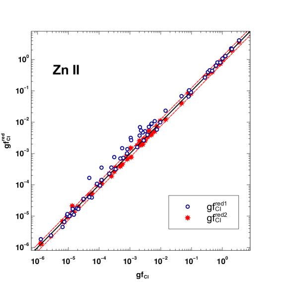
Figure 1: Comparison of the weighted oscillator strengths $gf$ determined in the CI_TRO to those determined in CI${}_{\mathrm{TRO}}^{\mathrm{red1}}$ and CI${}_{\mathrm{TRO}}^{\mathrm{red2}}$ approaches for Zn II. Dashed lines show the 25% deviation limits.

Using the determined CI wavefunction expansions, we are able to generate data sets for the radiative transitions involving twenty seven energy levels. In Fig. 1 we compare the weighted oscillator strengths determined in approximation CI_TRO with $gf$ values determined in CI${}_{\mathrm{TRO}}^{\mathrm{red1}}$ and CI${}_{\mathrm{TRO}}^{\mathrm{red2}}$ approximations. Although there are some weaker lines where deviations can exceed $25\%$, especially in CI${}_{\mathrm{TRO}}^{\mathrm{red2}}$ approximation, for most lines the agreement is within the range of $25\%$. One can notice that the deviations have become significantly smaller in CI${}_{\mathrm{TRO}}^{\mathrm{red1}}$ approximation, indicating the convergence of the $gf$ values, as it has been a case with level energy values (see Table 1).

Table 2: Transition line strengths $S$ (in a.u.) for Zn II determined in the CI_TRO approximation.

Data	Type	$N_{l}$	$N_{u}$	$S$
S	E1	1	2	4.199E$+$00
S	E1	1	3	8.401E$+$00
S	M2	1	3	1.405E$+$02
S	E2	1	4	1.525E$+$00
S	E2	1	5	9.898E$-$01
S	M1	1	6	1.115E$-$06
S	E2	1	7	6.011E$+$01
S	E2	1	8	9.013E$+$01
S	E1	1	9	1.001E$-$02
S	E1	1	10	1.593E$-$02
S	M2	1	10	2.201E$-$02
S	E3	1	11	9.030E$-$06
S	M2	1	11	1.250E$+$01
S	E1	1	12	2.970E$-$02
S	M2	1	12	2.061E$+$00
S	E2	2	3	1.278E$+$02
S	M1	2	3	1.300E$+$00
S	E3	2	4	3.139E$+$00
S	M2	2	4	8.302E$-$03
S	E1	2	5	1.196E$-$02
S	M2	2	5	7.790E$-$03
S	E1	2	6	2.822E$+$00
S	E1	2	7	1.317E$+$01
S	M2	2	7	8.199E$+$00

Note. — The first column describes the transition data type (S: line strength $S$, A: transition probability $A$). The second column describes transition line type, $N_{l}$ is for the lower level index, $N_{u}$ denotes the upper level index.

Note. — (This table is available in its entirety in a machine-readable form in the online journal. A portion is shown here for guidance regarding its form and content.)

Table 2 gives a sample of the transition parameters used in the plasma simulation package Cloudy. Here transition line strengths $S$ are tabulated together with the type of transition ($E1$, $E2$, $E3$, $M1$, $M2$). The line strengths $S$ are preferred as they do not depend explicitly on the transition energy $\Delta E$. For the further use, oscillator strengths $f$ or transition probabilities $A$ can be derived using well-known relations. A complete table of transition parameters is available on-line.

Table 3: Transition vacuum wavelengths (in Å), the upper levels, oscillator strengths $gf$ and transition probabilities $A$ (in s^-1) for Zn II, including some commonly observed lines.

$\lambda$ (Å)	Upper level	$gf$	$A$
2062.6604	$3d^{10}4p$ ${}^{2}P_{1/2}$	6.18E$-$1	4.85E$+$8
2026.1370	$3d^{10}4p$ ${}^{2}P_{3/2}$	1.26E$+$0	5.12E$+$8
986.5237	$3d^{10}5p$ ${}^{2}P_{1/2}$	3.08E$-$3	1.06E$+$7
984.1414	$3d^{10}5p$ ${}^{2}P_{3/2}$	4.92E$-$3	8.46E$+$6
949.4630	$3d^{9}4s4p$ ${}^{4}P_{3/2}$	9.50E$-$3	1.76E$+$7
938.7130	$3d^{9}4s4p$ ${}^{4}P_{1/2}$	3.65E$-$3	1.38E$+$7
923.9760	$3d^{9}4s4p$ ${}^{4}F_{3/2}$	9.17E$-$6	1.79E$+$4

Note. — All these lines originate from the ground level $3d^{10}4s$ ${}^{2}S_{1/2}$ ($g=2$). The statistical weights $g=2J+1$ of the upper levels are given in Table 1.

In Table 3 we provide the transition wavelengths $\lambda$, oscillator strengths $gf$, and $A$ values for several observed lines. We note that for 5 of these lines, no $gf$ or $A$ values are listed in Morton (2003).

Along with the radiative transition data, we have determined electron-impact excitation parameters for these lines in the plane-wave Born approximation. The methods and codes for such calculation are described by Bogdanovich et al. (2014). We present just a sample of the collisional parameters in Table 4, whereas the complete version of the table is available on-line. We note that the approximation adopted in our calculations can not produce highly accurate data for the electron-impact excitation process. Nevertheless, as the more accurate calculations for this level set of Zn II are absent, our data are an improvement over other more rough approximations, such as g-bar approximation.

As already mentioned in Sect. 1.2, several elaborate studies on the Zn II ion electron-impact excitation were published, see Pindzola et al. (1991); Zatsarinny & Bandurina (1999); Sharma et al. (2011). Since their data are incompatible with our model due to a different atomic structure, a narrow energy range (as in Pindzola et al. (1991); Zatsarinny & Bandurina (1999)), and a different data type, when only excitation cross sections are plotted instead of collision rates, we cannot include those data into our data set or perform a comprehensive comparison with our data. Some qualitative assesment suggests that our data deviate no more than $30\%$ from the R-matrix or relativistic distorted-wave results at low electron energies for the optically allowed transitions and no more than $45\%$ for the forbidden transitions. At high electron energies, these deviations decrease at least twofold.

The ab initio calculation results for the level energies $E$, the radiative transition parameters - oscillator strengths $gf$, transition line strengths $S$, transition probabilities $S$, and the radiative lifetimes $\tau$ for the Zn II are available from the database ADAMANT (http://www.adamant.tfai.vu.lt/database) being developed at Vilnius University.

We note in passing that the theoretical calculations of the transition wavelengths can never be as accurate as the experimental data. We have therefore used the experimental $\lambda$ values in our Cloudy simulation runs, as has been done in previous studies. The oscillator strengths or transition probabilities need to be corrected for the difference between the experimental and theoretical energies. We have indeed corrected the transition rates by using the experimental level energies to determine the radiative transition parameters (e.g., the transition probabilities $A$ or the oscillator strengths $gf$).

Table 4: Table 4: Effective collision strengths $\Upsilon$ for the electron-impact excitation of Zn II at 14 selected temperatures determined in the plane-wave Born approximation.

		Electron Temperatures (K)
$N_{l}$	$N_{up}$	$4\times 10^{2}$	$8\times 10^{2}$	$2\times 10^{3}$	$4\times 10^{3}$	$8\times 10^{3}$	$2\times 10^{4}$	$4\times 10^{4}$	$8\times 10^{4}$	$2\times 10^{5}$	$4\times 10^{5}$	$8\times 10^{5}$	$2\times 10^{6}$	$4\times 10^{6}$	$8\times 10^{6}$
1	2	2.29E$+$0	2.29E$+$0	2.30E$+$0	2.38E$+$0	2.67E$+$0	3.58E$+$0	4.78E$+$0	6.46E$+$0	9.42E$+$0	1.22E$+$1	1.52E$+$1	1.97E$+$1	2.34E$+$1	2.72E$+$1
1	3	4.53E$+$0	4.53E$+$0	4.55E$+$0	4.70E$+$0	5.26E$+$0	7.07E$+$0	9.45E$+$0	1.28E$+$1	1.87E$+$1	2.41E$+$1	3.03E$+$1	3.92E$+$1	4.65E$+$1	5.41E$+$1
1	4	6.93E$-$2	6.93E$-$2	6.94E$-$2	7.05E$-$2	7.57E$-$2	9.37E$-$2	1.15E$-$1	1.40E$-$1	1.67E$-$1	1.82E$-$1	1.92E$-$1	1.99E$-$1	2.02E$-$1	2.03E$-$1
1	5	4.67E$-$2	4.67E$-$2	4.67E$-$2	4.74E$-$2	5.06E$-$2	6.22E$-$2	7.64E$-$2	9.23E$-$2	1.10E$-$1	1.20E$-$1	1.26E$-$1	1.31E$-$1	1.33E$-$1	1.35E$-$1
1	6	3.17E$-$1	3.17E$-$1	3.17E$-$1	3.19E$-$1	3.33E$-$1	4.07E$-$1	5.22E$-$1	6.84E$-$1	9.39E$-$1	1.13E$+$0	1.29E$+$0	1.45E$+$0	1.54E$+$0	1.59E$+$0
1	7	3.13E$-$1	3.13E$-$1	3.13E$-$1	3.14E$-$1	3.25E$-$1	3.85E$-$1	4.81E$-$1	6.20E$-$1	8.41E$-$1	1.01E$+$0	1.16E$+$0	1.30E$+$0	1.38E$+$0	1.43E$+$0
1	8	4.68E$-$1	4.68E$-$1	4.68E$-$1	4.70E$-$1	4.86E$-$1	5.76E$-$1	7.21E$-$1	9.29E$-$1	1.26E$+$0	1.51E$+$0	1.73E$+$0	1.95E$+$0	2.06E$+$0	2.14E$+$0
1	9	1.02E$-$1	1.02E$-$1	1.02E$-$1	1.02E$-$1	1.04E$-$1	1.16E$-$1	1.32E$-$1	1.51E$-$1	1.74E$-$1	1.86E$-$1	1.93E$-$1	2.00E$-$1	2.05E$-$1	2.11E$-$1
2	3	1.76E$-$1	2.85E$-$1	5.68E$-$1	9.45E$-$1	1.48E$+$0	2.35E$+$0	2.99E$+$0	3.48E$+$0	3.87E$+$0	4.02E$+$0	4.11E$+$0	4.16E$+$0	4.18E$+$0	4.19E$+$0
2	4	8.77E$-$7	8.87E$-$7	9.69E$-$7	1.13E$-$6	1.36E$-$6	1.72E$-$6	2.03E$-$6	2.37E$-$6	2.82E$-$6	3.09E$-$6	3.28E$-$6	3.41E$-$6	3.46E$-$6	3.49E$-$6
2	5	1.15E$-$5	1.16E$-$5	1.27E$-$5	1.54E$-$5	2.07E$-$5	3.21E$-$5	4.27E$-$5	5.27E$-$5	6.27E$-$5	7.41E$-$5	2.86E$-$4	2.61E$-$3	7.28E$-$3	1.44E$-$2
2	6	2.67E$-$1	2.67E$-$1	2.72E$-$1	3.06E$-$1	4.25E$-$1	8.37E$-$1	1.45E$+$0	2.40E$+$0	4.26E$+$0	6.10E$+$0	8.23E$+$0	1.14E$+$1	1.41E$+$1	1.67E$+$1
2	7	2.21E$-$5	2.21E$-$5	2.25E$-$5	2.69E$-$5	4.83E$-$5	1.55E$-$4	3.74E$-$4	8.11E$-$4	1.88E$-$3	3.12E$-$3	5.07E$-$3	1.41E$-$1	1.28E$+$0	4.88E$+$0

Note. — (This table is available in its entirety in a machine-readable form in the online journal. A portion is shown here for guidance regarding its form and content.)

3 Cloudy calculations

3.1 Application to DLAs and Sub-DLAs

One of the motivations behind our interest in the Zn II atomic data stems from the somewhat surprising results obtained from observations of Zn II lines in DLAs and sub-DLAs. We now describe these results and discuss the implications of our revised atomic data for the evolution of DLAs/ sub-DLAs.

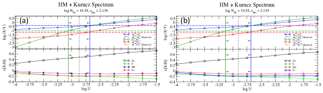
Figure 2: Comparison of the ionization corrections and ionization parameters derived for the sub-DLA toward Q1039-2719 with Cloudy version C13.02 (a) before and (b) after incorporating our revised atomic data for Zn II.

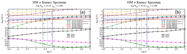
Figure 3: Comparison of the ionization corrections and ionization parameters derived for the sub-DLA toward Q2123-0050 with Cloudy version C13.02 (a) before and (b) after incorporating our revised atomic data for Zn II.

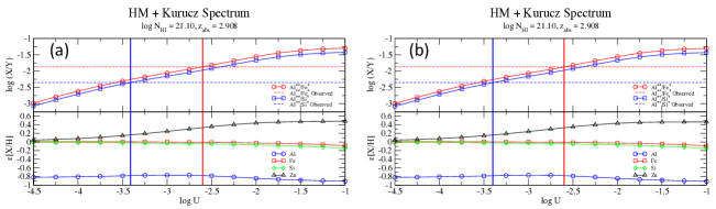
Figure 4: Comparison of the ionization corrections and ionization parameters derived for the DLA toward Q2342+34 with Cloudy version C13.02 (a) before and (b) after incorporating our revised atomic data for Zn II.

Most models of chemical evolution predict a near-solar mean interstellar metallicity for galaxies at redshifts $z\sim 0$ [e.g., Pei et al. (1999); Somerville et al. (2001)]. Surprisingly, DLAs at $z<1.5$ evolve little if at all, with metallicities far below the predictions of models based on the cosmic star formation history [e.g., Pettini et al. (1999); Kulkarni & Fall (2002); Prochaska et al. (2003, 2007); Khare et al. (2004); Kulkarni et al. (2005, 2007, 2010); Péroux et al. (2008)]. The DLA global mean metallicity shows some evolution at high z, but seems to reach only about $20\%$ of the solar level by $z=0$. These results appear to contradict the near-solar mass-weighted mean metallicity at $z\sim 0$ predicted by most models and observed in nearby galaxies. Equally surprising, a significant fraction of sub-DLAs appear to be highly metal-rich (near-solar or super-solar), even at redshifts $z>2$ (e.g., Akerman et al. (2005); Péroux et al. (2006a, b, 2008), Prochaska et al. (2006); Meiring et al. (2007, 2008, 2009a, 2009b); Kulkarni et al. (2007, 2010); Nestor et al. (2008); Som et al. (2013, 2014)). The super-solar metallicities observed in many sub-DLAs (a large fraction of which are derived from Zn) are particularly striking, because no local counterparts to such systems are known among normal galaxies.

Given these surprising results, it is natural to ask to what extent the results are affected by ionization of the absorbing gas. Ionization corrections are likely to be especially important for sub-DLAs and low-$N_{\mathrm{H\,I}}$ DLAs. Cloudy calculations using existing atomic data suggest that the low-$N_{\mathrm{H}\,I}$ sub-DLAs can be significantly ionized, but give relatively small ionization corrections to the abundances ($\varepsilon(\mathrm{X})=\mathrm{[X/H]_{total}-[X\,II/[H\,I]}$) over the range of ionization parameters ($U=n_{\gamma}/n_{\mathrm{H}}=\Phi_{912}/cn_{\mathrm{H}}$, where $\Phi_{912}$ denotes the flux of radiation with h$\nu>$ 13.6 eV and $n_{\mathrm{H}}$ denotes the total gas density) allowed by observed ratios such as Al III/Al II, S III/S II, or Fe III/Fe II [e.g., Dessagues-Zavadsky et al. (2003), Dessagues-Zavadsky et al. (2004); Meiring et al. (2007, 2009b); Som et al. (2013, 2014)].

To illustrate the effect of ionization, we now show the Cloudy photoionization modeling calculations for a few illustrative absorbers. As typical examples of sub-DLAs, we choose the $z=2.139$ system toward Q1039-2719 and the $z=2.058$ system toward Q2123-0050. Both of these sub-DLAs have log $N_{\rm HI}=19.35$. As an example of DLAs, we use the $z=2.908$ absorber toward Q2342+34 with $\log N_{\rm HI}=21.10$. We assume that the ionizing radiation incident on the absorbing cloud is a combination of the extragalactic UV background and an O/B-type stellar radiation field. We adopt the extragalactic UV background from Haardt & Madau (1996) and Madau et al. (1999), evaluated at the absorber redshift. The O/B type stellar radiation field corresponds to a Kurucz model stellar spectrum for 30,000 K. The incident radiation field was taken to be a mixture of the extragalactic and O/B type stellar radiation fields in equal parts. Schaye (2006) has suggested that the contribution from local sources to the ionization of DLA absorbers may be significant when compared with the contribution from the extragalactic background ionizing radiation. Additionally, our simulations include the cosmic microwave background at the absorber redshift, and the cosmic ray background. However, we do not include the radiation from local shocks produced by supernovae, white dwarfs, or compact binary systems.

For each absorber, we first ran grids of photoionization models using Cloudy version C13.02 [Ferland et al. (2013)], by varying the ionization parameter from $10^{-6}$ to 1. The models were made to match the observed H I column density and the observed metallicity based on Zn II. Constraints on the ionization parameter were estimated by comparing the observed values of the column density ratios for various ions with the values calculated from our simulation grids. The ionization parameter thus estimated was used to obtain the ionization correction values to the abundances. In particular, we used column density ratios of adjacent ions of the same element, because they provide more reliable observational constraints than the ratios involving different elements, since the latter may be affected by differences in dust depletion or in nucleosynthesis. For the two illustrative absorbers discussed above toward Q1039-2719 and Q2123-0050, we estimate ionization parameters $\log U$ of -2.87 and -2.35, respectively. The corresponding estimates of ionization corrections for Zn II are 0.48 dex for the absorber toward Q1039-2719 and 0.59 dex for the absorber toward Q2123-0050, respectively. For S II, the corresponding ionization corrections are -0.20 dex and -0.30 dex, respectively. Figures 2a and 3a show the ionization corrections for several elements as a function of the ionization parameter for these models, and the range of $U$ allowed by the observed ion ratios in these absorbers. For the DLA toward Q2342+34, we estimate ionization parameter $\log U$ of -3.41 using Al III/Si II and Zn II ionization correction of +0.16 dex (Fig. 4a).

To assess the effect of our atomic data calculations, we next ran the revised Cloudy models that include our improved Zn atomic data for the illustrative DLA and sub-DLA absorbers discussed above. Figures 2b and 3b show the results for the ionization correction as a function of ionization parameter, and the range of $U$ allowed by the observed ion ratios. The ionization parameters are -2.90 and -2.38, respectively, for the absorbers toward Q1039-2719 and Q2123-0050. The corresponding ionization corrections for Zn II are 0.45 dex and 0.54 dex, respectively, i.e. lower than those obtained with Cloudy version C13.02 by 0.03 dex and 0.05 dex, respectively. For the DLA toward Q2342+34, we estimate ionization parameter $\log U$ of -3.40 using Al III/Si II and Zn II ionization correction of +0.16 dex (Fig. 4b).

Combining the difference in ionization correction with the difference in $N_{\rm Zn\,II}$ implied by the revised oscillator strengths (which are lower by 0.10 dex), the revised [Zn/H] values for the above sub-DLA absorbers would be lower by $0.13-0.15$ dex compared to the values based on the previously available atomic data. For the DLA absorber, the revised [Zn/H] value would be lower by 0.10 dex compared to the values based on the previous atomic data.

We note, however, that the estimates of ionization corrections are sensitive to the adopted values of dielectronic recombination rates, which are unknown for ions of most elements in the third row of the periodic table and beyond, including key elements such as Al, Fe, Zn. In future papers, we plan to address the dielectronic recombination rates.

3.2 Emission lines

The atomic data described in this paper will be part of the next release of Cloudy. For reference, Figure 5 shows the lowest energy levels and indicates some of the stronger lines with their air wavelengths given in Å. We know of no calculations of the emission spectra that demonstrates its diagnostic power, so we do representative calculations here.

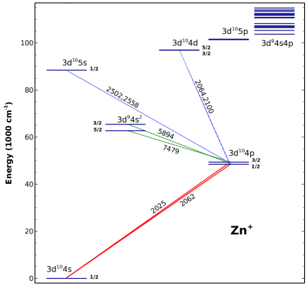
Figure 5: The diagram of the lowest levels for Zn II, showing the even-parity configuration $3d^{10}4s$, $3d^{10}5s$, $3d^{10}4d$, $3d^{9}4s^{2}$ levels and the odd-parity configuration $3d^{10}4p$, $3d^{9}4s4p$ levels. The strongest lines originating from the $3d^{10}4p-3d^{10}4s$ transition (solid lines) and from the $3d^{9}4s^{2}-3d^{10}4p$ transition (dashed lines) are also plotted. Other strong doublet E1 lines, representing transitions $3d^{10}5s-3d^{10}4p$ (dotted line) and $3d^{10}4d-3d^{10}4p$ (dash-dotted line) are also shown.

Figure 6 shows Zn II emission spectra at a temperature of 10⁴ K and electron densities of 1 and 10¹⁰ cm^-3. The gas was assumed to be composed entirely of Zn⁺ with no incident SED, so the emission is entirely due to electron impact excitation. The strongest lines, as expected, are the $3d^{10}4p\;^{2}P_{3/2,1/2}-3d^{10}4s\;^{2}S_{1/2}$ doublet at $\lambda\lambda$ 2025.48Å, 2062.00Å. The next stronger lines are $3d^{9}4s^{2}\;{}^{2}D_{5/2}-3d^{10}4p\;^{2}P_{3/2}$   at 7478.82Å  and $3d^{9}4s^{2}\;{}^{2}D_{3/2}-3d^{10}4p\;^{2}P_{1/2}$  at 5894.37Å. These lines are considerably fainter but are important because they can be detected with large ground-based instruments. The same is true for the E1 doublet lines $3d^{10}5s\;^{2}S_{1/2}-3d^{10}4p\;^{2}P_{1/2,3/2}$ at $\lambda\lambda$ 2501.99Å, 2559.95Å  and the doublet of the lines at $\lambda\lambda$ 2064.23Å, 2099.94Å, representing the E1 transitions $3d^{10}4d-3d^{10}4p$.

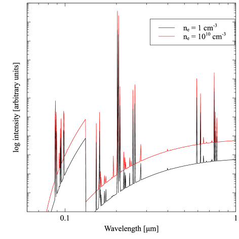
Figure 6: The Zn II strongest line and continuum emission. The gas has only Zn⁺ at 10⁴ K and is computed at two densities. The vertical scale is adjusted so that the two spectra lie near one another, so the vertical scale is arbitrary. Both Zn II recombination and brews emission are present.

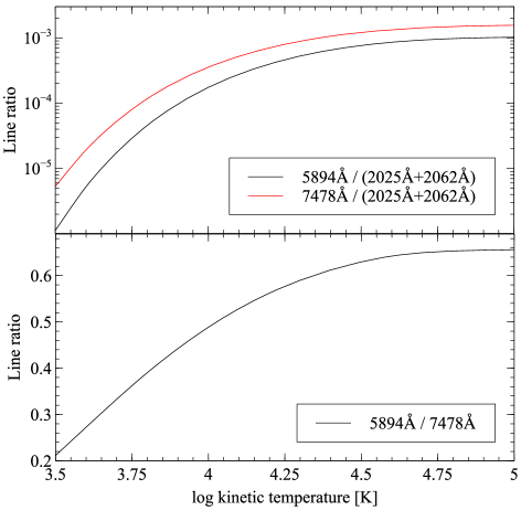
Figure 7: Several Zn II temperature indicators are shown.

Figure 7 shows several possible Zn II temperature indicators. To do this, the kinetic temperature of a pure Zn⁺ gas with an electron density of 1 cm^-3 was varied over a wide range and the emission ratios suggested by Figure 5 plotted.

The upper panel shows the ratio of the two optical lines relative to the sum of the two strongest UV lines. This is an indicator with a wide dynamic range although the plot also shows that the optical lines are far fainter than the UV transitions. The lower panel shows the ratio of the two optical lines. These have the advantage of being detectable by ground-based instrumentation.

4 Conclusions

Our estimates of the oscillator strengths for the key Zn II absorption lines at 2026.14, 2062.66 Å are higher than the previous values by 0.1 dex, implying the Zn II column densities inferred from these lines to be lower by 0.1 dex. Moreover, the sub-DLA ionization corrections for Zn II would be lower by $\sim 0.03-0.05$ dex, as discussed in section 3.1. Thus, the logarithmic metallicities inferred from these lines would be lower by $0.13-0.15$ dex for sub-DLAs and by 0.1 dex for DLAs, compared to past studies. While differences of this amount are significant, they are not adequate to explain why the sub-DLA metallicities are so much higher than that of DLAs.

Using Cloudy simulations, we have demonstrated some astrophysical applications of our atomic data calculations, and the predictions for many emission and absorption lines. One can compare such predictions with the observed line strengths to obtain improved constraints on the chemical composition and physical properties of the Galactic and extragalactic ISM. Past observations of Zn II absorption in the Galactic ISM and the DLAs/sub-DLAs have targeted the $\lambda\lambda 2026.14,2062.66$ lines. Our new calculations show that these are indeed the strongest observable lines in the commonly accessible wavelength region. Our complete set of Zn II oscillator strengths (available online) contains many UV transitions. Although most of these transitions are weak, some of them may be detectable in high-S/N spectra obtained with the extremely large telescopes of the future.

References

- Akerman et al. (2005) Akerman, C. J., Ellison, S. L., Pettini, M., & Steidel, C. C. 2005, A&A, 440, 499
- Battisti et al. (2012) Battisti, A. J., et al. 2012, ApJ, 744, 93
- Bergeson & Lawler (1993) Bergeson, S. D., & Lawler, J. E. 1993, ApJ, 408, 382
- Bogdanovich (2004) Bogdanovich, P. 2004, Lithuan. J. Phys., 44, 135
- Bogdanovich (2005) Bogdanovich, P. 2005, Nuclear Instr. Meth. B, 235, 92
- Bogdanovich & Karpuškienė (1999) Bogdanovich, P., & Karpuškienė, R. 1999, Lithuan J. Phys., 39, 193
- Bogdanovich & Karpuškienė (2001) Bogdanovich, P., & Karpuškienė, R. 2001, Comput. Phys. Commun., 134, 231
- Bogdanovich et al. (2002) Bogdanovich, P., Karpuškienė, R., & Momkauskaitė, A. 2002, Comput. Phys. Commun., 143, 174
- Bogdanovich et al. (2003a) Bogdanovich, P., Karpuškienė, R.,& Martinson, I. 2003, Phys. Scripta, 67, 44
- Bogdanovich et al. (2003b) Bogdanovich, P., Karpuškienė, R.,& Udris, A. 2003, Phys. Scripta, 67, 395
- Bogdanovich et al. (2014) Bogdanovich, P., Kisielius, R., & Stonys, D. 2014, Lithuan. J Phys., 54, 67
- Bogdanovich & Martinson (1999) Bogdanovich, P., & Martinson, I. 2003, Phys. Scripta, 60, 217
- Bogdanovich & Momkauskaitė (2004) Bogdanovich, P., & Momkauskaitė, A. 2004, Comput. Phys. Commun., 157, 217
- Çelik et al. (2013) Çelik, G., Erol, E., & Tasfer, M. 2013, JQSRT, 129, 263
- Chen et al. (2005) Chen, H.-W., Prochaska, J. X., Bloom, J. S., & Thompson, I. B. 2005, ApJ, 634, L25
- Chou & Johnson (1997) Chou, H.-S., & Johnson, W. R. 1997, Phys. Rev. A, 56, 2424
- Cooke et al. (2011) Cooke, R., Pettini, M., Steidel, C. C., Rudie, G. C., & Nissen, P. E. 2011, MNRAS, 417, 1534
- Cowan (1981) Cowan, R. D. The Theory of Atomic Structure and Spectra University of California Press, Los Angeles, 1981
- Dessagues-Zavadsky et al. (2003) Dessauges-Zavadsky, M., Péroux, C., Kim, T.-S., D’Odorico, S., & McMahon, R. G. 2003, MNRAS, 345,447
- Dessagues-Zavadsky et al. (2004) Dessauges-Zavadsky, M., Calura, F., Prochaska, J. X., D’Odorico, S., & Matteucci, F. 2004, A&A, 416, 79
- Ferland et al. (2013) Ferland, G. J., Porter, R. L., van Hoof, P. A. M., et al. 2013, Rev. Mexicana Astron. Astrofis., 49, 1
- Froese Fischer (1987) Froese Fischer, C. 1977, J. Phys. B, 10, 1241
- Froese Fischer (1987) Froese Fischer, C. 1987, Comput. Phys. Commun., 43, 355
- Froese Fischer & Godefroid (1991) Froese Fischer, C., & Godefroid, M.R. 1991, Comput. Phys. Commun., 64, 501
- Froese Fischer et al. (1991) Froese Fischer, C., Godefroid, M.R., & Hibbert, A. 1991, Comput. Phys. Commun., 64, 486
- Fynbo et al. (2009) Fynbo, J. P. U, Jakobsson, P., Prochaska, J. X., et al. 2009, ApJS, 185, 526
- Gaigalas et al. (1997) Gaigalas, G., Rudzikas, Z.R., Froese Fischer, C. 1997, J. Phys. B, 30, 3347
- Gaigalas et al. (1998) Gaigalas, G., Rudzikas, Z.R., Froese Fischer, C. 1998, At. Data Nucl. Data Tables, 70, 1
- Guimaraes (2012) Guimaraes, R., Noterdaeme, P., Petitjean, P., et al. 2012, AJ, 143, 147
- Gullberg & Litzén (2000) Gullberg, D., & Litzén, U. 2000, Phys. Scripta, 61, 652
- Haardt & Madau (1996) Haardt, F., & Madau, P. 1996, ApJ, 461, 20
- Harrison & Hibbert (2003) Harrison, S.A., & Hibbert, A. 2003, MNRAS, 340, 1279
- Hibbert et al. (1991) Hibbert, A., Glass, R., Froese Fischer, C. 1991, Comput. Phys. Commun., 64, 445
- Howk & Sembach (1999) Howk, J. C., & Sembach, K. R. 1999, ApJ, 523, L141
- Jenkins (2009) Jenkins, E. B. 2009, ApJ, 700, 1299
- Jorgenson et al. (2013) Jorgenson, R. A., Murphy, M. T., & Thompson, R. 2013, MNRAS, 435, 482
- Karpuškienė & Bogdanovich (2001) Karpuškienė, R., & Bogdanovich, P. 2001, LithJP, 41, 174
- Karpuškienė & Bogdanovich (2003) Karpuškienė, R., & Bogdanovich, P. 2003, J. Phys. B, 36, 2145
- Karpuškienė et al. (2013) Karpuškienė, R., Bogdanovich, P., & Kisielius, R. 2013, Phys. Rev. A, 88, 022519
- Khare et al. (2004) Khare, P., Kulkarni, V. P., Lauroesch, J. T., York, D. G., Crotts, A. P. S., & Nakamura, O. 2004, ApJ, 616, 86
- Kisielius et al. (2014) Kisielius, R., Kulkarni V. P., Ferland, G. J., Bogdanovich P., & Lykins M. L. 2014, ApJ, 780, 76
- Kramida et al. (2014) Kramida, A., Ralchenko, Y., Reader, J., and NIST ASD Team 2014, NIST Atomic Spectra Database (version 5.2), http://physics.nist.gov/asd National Institute of Standards and Technology, Gaithersburg, MD
- Kulkarni & Fall (2002) Kulkarni, V. P., & Fall, S. M. 2002, ApJ, 580, 732
- Kulkarni et al. (2005) Kulkarni, V. P., Fall, S. M., Lauroesch, J. T., York, D. G., Welty, D. E., Khare, P., Truran, J. W. 2005, ApJ, 618, 68
- Kulkarni et al. (2007) Kulkarni, V. P., Khare, P., Péroux, C., et al. 2007, ApJ, 661, 88
- Kulkarni et al. (2010) Kulkarni, V. P., Khare, P., Som, D., Meiring, J., York, D. G., Péroux, C., & Lauroesch, J. T. 2010, NewA, 15, 735
- Kulkarni et al. (2012) Kulkarni, V. P., Meiring, J., Som, D., et al. 2012, ApJ, 749, 176
- Kupliauskienė et al. (2006) Kupliauskienė A., Bogdanovich, P., Borovik, A.A., Zatsarinny, O.I., Grum-Grzhimailo, A.N., & Bartschat, K. 2006, J. Phys. B, 39, 591
- Lykins et al. (2013) Lykins, M. L., Ferland, G. J., Porter, R. L., et al. 2013, MNRAS, 429, 3133
- Lykins et al. (2014) Lykins, M. L., Ferland, G. J., Kisielius R., et al. 2015, ApJ, submitted
- Madau et al. (1999) Madau, P., Haardt, F., & Rees, M. J. 1999, ApJ, 514, 648
- Mayo et al. (2006) Mayo, R., Ortiz, M., & Campos, J. 2006, Eur. Phys. J. D, 37, 181
- Meiring et al. (2007) Meiring, J. D., Lauroesch, J. T., Kulkarni, V. P., Péroux, C., Khare, P., York, D. G., & Crotts, A. P. S. 2007, MNRAS, 376, 557
- Meiring et al. (2008) Meiring, J. D., Kulkarni, V. P., Lauroesch, J. T., Péroux, C., Khare, P., York, D. G., & Crotts, A. P. S. 2008, MNRAS, 384, 1015
- Meiring et al. (2009a) Meiring, J. D., Kulkarni, V. P., Lauroesch, J. T., Péroux, C., Khare, P., & York, D. G. 2009a, MNRAS, 393, 1513
- Meiring et al. (2009b) Meiring, J. D., Lauroesch, J. T., Kulkarni, V. P., Péroux, C., Khare, P., & York, D. G. 2009b, MNRAS, 397, 2037
- Meyer (1989) Meyer, D. M., Welty, D. E. & York, D. G. 1989, ApJ, 343, L37
- Morton (2003) Morton, D. C. 2003, ApJS, 149, 205
- Nestor et al. (2008) Nestor, D. B., Pettini, M., Hewett, P. C., Rao, S., & Wild, V. 2008, MNRAS, 390, 1670
- Noterdaeme et al. (2012) Noterdaeme, P., Petitjean, P., Carithers, W. C., et al. 2012, A&A, 547, L1
- Osterbrock & Ferland (2006) Osterbrock, D. E., & Ferland, G. J. 2006, Astrophysics of Gaseous Nebulae & Active Galactic Nuclei, 2nd Ed. (Mill Valley; University Science Press) (AGN3)
- Pei et al. (1999) Pei, Y. C., Fall, S. M., & Hauser, M. G. 1999, ApJ, 522, 604
- Péroux et al. (2005) Péroux, C., Dessauges-Zavadsky, M., D’Odorico, S., et al. 2005, MNRAS, 363, 479
- Péroux et al. (2006a) Péroux, C., Kulkarni, V. P., Meiring, J., Ferlet, R., Khare, P., Lauroesch, J. T., Vladilo, G., & York, D. G. 2006a, A&A, 450, 53
- Péroux et al. (2006b) Péroux, C., Meiring, J. D., Kulkarni, V. P., Ferlet, R., Khare, P., Lauroesch, J. T., Vladilo, G., & York, D. G. 2006b, MNRAS, 372, 369
- Péroux et al. (2008) Péroux, C., Meiring, J. D., Kulkarni, V. P., et al. 2008, MNRAS, 386, 2209
- Pettini et al. (1994) Pettini, M., Smith, L. J., Hunstead, R. W., & King, D. L. 1994, ApJ, 426, 79
- Pettini et al. (1995) Pettini, M., Lipman, K., & Hunstead, R. W. 1995, ApJ, 451, 100
- Pettini et al. (1997) Pettini, M., Smith, L. J., King, D. L., & Hunstead, R. W. 1997, ApJ, 486, 665
- Pettini et al. (1999) Pettini, M., Ellison, S. L., Steidel, C. C., & Bowen, D. V. 1999, ApJ, 510, 576
- Pindzola et al. (1991) Pindzola, M. S., Badnell, N. R., Henry, R. J. W., Griffin, D. C., & van Wyngaarden, W. L. 1991, Phys. Rev. A, 44, 5628
- Prochaska et al. (2003) Prochaska, J. X., Gawiser, E., Wolfe, A. M., Castro, S., & Djorgovski, S. G. 2003, ApJ, 595, L9
- Prochaska et al. (2005) Prochaska, J. X., Herbert-Fort, S., & Wolfe, A. M. 2005, ApJ, 635, 123
- Prochaska et al. (2006) Prochaska, J. X., O’Meara, J. M., Herbert-Fort, S., Burles, S., Prochter, G. E., & Bernstein, R. A. 2006, ApJ, 648, L97
- Prochaska et al. (2007) Prochaska, J. X., Chen, H.-W., Dessauges-Zavadsky, M., et al. 2007a, ApJ, 666, 267
- Rafelski et al. (2012) Rafelski, M., Wolfe, A. M., Prochaska, J. X., Neeleman, M., & Mendez, A. J. 2012, ApJ, 755, 89
- Savage & Sembach (1996) Savage, B. D., & Sembach, K. R. 1996, ARAA, 34, 279
- Savaglio et al. (2003) Savaglio, S., Fall, S. M., & Fiore, F. 2003, ApJ, 585, 638
- Schaye (2006) Schaye, J. 2006, ApJ, 643, 59
- Sharma et al. (2011) Sharma, I., Surzhykov A., Srivastava, R., & Fritzsche, S. 2011, Phys. Rev. A, 83, 062701
- Som et al. (2013) Som, D., Kulkarni, V. P., Meiring, J., et al. 2013, MNRAS, 435, 1469
- Som et al. (2014) Som, D., Kulkarni, V. P., Meiring, J., et al. 2015, ApJ, submitted
- Somerville et al. (2001) Somerville, R. S., Primack, J. R., & Faber, S. M. 2001, MNRAS, 320, 504
- Storrie-Lombardi & Wolfe (2000) Storrie-Lombardi, L. J., & Wolfe, A. M. 2000, ApJ, 543, 552
- Zafar et al. (2013) Zafar, T., Péroux, C., Popping, A., et al. 2013, A&A, 556, 141
- Zatsarinny & Bandurina (1999) Zatsarinny, O., & Bandurina, L. 1999, J. Phys. B, 32, 4793