Global bifurcations close to symmetry

Abstract.

Heteroclinic cycles involving two saddle-foci, where the saddle-foci share both invariant manifolds, occur persistently in some symmetric differential equations on the 3-dimensional sphere. We analyse the dynamics around this type of cycle in the case when trajectories near the two equilibria turn in the same direction around a 1-dimensional connection — the saddle-foci have the same chirality. When part of the symmetry is broken, the 2-dimensional invariant manifolds intersect transversely creating a heteroclinic network of Bykov cycles.

We show that the proximity of symmetry creates heteroclinic tangencies that coexist with hyperbolic dynamics. There are $n$-pulse heteroclinic tangencies — trajectories that follow the original cycle $n$ times around before they arrive at the other node. Each $n$-pulse heteroclinic tangency is accumulated by a sequence of $(n+1)$-pulse ones. This coexists with the suspension of horseshoes defined on an infinite set of disjoint strips, where the first return map is hyperbolic. We also show how, as the system approaches full symmetry, the suspended horseshoes are destroyed, creating regions with infinitely many attracting periodic solutions.

1. Introduction

A Bykov cycle is a heteroclinic cycle between two hyperbolic saddle-foci of different Morse index, where one of the connections is transverse and the other is structurally unstable — see Figure 1. There are two types of Bykov cycle, depending on the way the flow turns around the two saddle-foci, that determine the chirality of the cycle. Here we study the non-wandering dynamics in the neighbourhood of a Bykov cycle where the two nodes have the same chirality. This is also studied in [34], and the case of different chirality is discussed in [36]. A simplified version of the arguments presented here appears in [35].

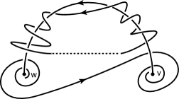
Figure 1. A Bykov cycle with nodes of the same chirality. There are two possibilities for the geometry of the flow around a Bykov cycle depending on the direction trajectories turn around the connection $[{\rm\bf v}\rightarrow{\rm\bf w}]$. We assume here that the nodes have the same chirality: trajectories turn in the same direction around the connection. When the endpoints of a nearby trajectory are joined, the closed curve is always linked to the cycle.

1.1. The object of study

Our starting point is a fully $({\rm\bf Z}_{2}\times{\rm\bf Z}_{2})$-symmetric differential equation $\dot{x}=f_{0}(x)$ in the three-dimensional sphere ${\rm\bf S}^{3}$ with two saddle-foci that share all the invariant manifolds, of dimensions one and two, both contained in flow-invariant submanifolds that come from the symmetry. This forms an attracting heteroclinic network $\Sigma^{0}$ with a non-empty basin of attraction $V^{0}$. We study the global transition of the dynamics from this fully symmetric system $\dot{x}=f_{0}(x)$ to a perturbed system $\dot{x}=f_{\lambda}(x)$, for a smooth one-parameter family that breaks part of the symmetry of the system. For small perturbations the set $V^{0}$ is still positively invariant.

When $\lambda\neq 0$, the one-dimensional connection persists, due to the remaining symmetry, and the two dimensional invariant manifolds intersect transversely, because of the symmetry breaking. This gives rise to a network $\Sigma^{\lambda}$, that consists of a union of Bykov cycles, contained in $V^{0}$. For partial symmetry-breaking perturbations of $f_{0}$, we are interested in the dynamics in the maximal invariant set contained in $V^{0}$. It contains, but does not coincide with, the suspension of horseshoes accumulating on $\Sigma^{\lambda}$ described in [3, 31, 34, 46]. Here, we show that close to the fully symmetric case it contains infinitely many heteroclinic tangencies. Under an additional assumption, we show that $V_{0}$ contains attracting limit cycles with long periods, coexisting with sets with positive entropy.

1.2. History

Homoclinic and heteroclinic bifurcations constitute the core of our understanding of complicated recurrent behaviour in dynamical systems. This starts with Poincaré on the late $19^{th}$ century, with major subsequent contributions by the schools of Andronov, Shilnikov, Smale and Palis. These results rely on a combination of analytical and geometrical tools used to understand the qualitative behaviour of the dynamics.

Heteroclinic cycles and networks are flow-invariant sets that can occur robustly in dynamical systems with symmetry, and are frequently associated with intermittent behaviour. The rigorous analysis of the dynamics associated to the structure of the nonwandering sets close to heteroclinic networks is still a challenge. We refer to [28] for an overview of heteroclinic bifurcations and for details on the dynamics near different kinds of heteroclinic cycles and networks.

Bykov cycles have been found analytically in the Lorenz model in [1, 44] and the nearby dynamics was studied by Bykov in in [9, 10, 11]. The point in parameter space where this cycle occurs is called a T-point in [18]. Recently, there has been a renewal of interest in this type of heteroclinic bifurcation in the reversible [15, 16, 37], equivariant [3, 34, 48] and conservative cases [7]. See also [31].

The transverse intersection of the two-dimensional invariant manifolds of the two equilibria implies that the set of trajectories that remain for all time in a small neighbourhood of the Bykov cycle contains a locally-maximal hyperbolic set admitting a complete description in terms of symbolic dynamics, reminiscent of the results of Shilnikov [52]. An obstacle to the global symbolic description of these trajectories is the existence of tangencies that lead to the birth of stable periodic solutions, as described for the homoclinic case in [2, 17, 40, 41, 54].

All dynamical models with quasi-stochastic attractors were found, either analytically or by computer simulations, to have tangencies of invariant manifolds [2, 21, 22]. As a rule, the sinks in a quasi-stochastic attractor have very long periods and narrow basins of attraction, and they are hard to observe in applied problems because of the presence of noise [24].

Motivated by the analysis of Lamb et al [37] in the context of the Michelson system, Bykov cycles have been considered by Knobloch et al [31]. Using the Lin’s method, the authors extend the analysis to cycles in spaces of arbitrary dimension, while restricting it to trajectories that remain for all time inside a small tubular neighbourhood of the cycle. We also refer the reader to [32], where the authors consider non-elementary $T$-points in reversible differential equations. The leading eigenvalues at the two equilibria are real and the two-dimensional invariant manifolds meet tangentially. They found chaos in the unfolding of this $T$-point and bifurcations of periodic solutions in the process of annihilation of the shift dynamics.

Bykov cycles appear in many applications like the Kuramoto-Sivashinsky systems [15, 37], magnetoconvection [46, 50] and travelling waves in reaction-diffusion dynamics [6, 26].

1.3. Chirality

For a Bykov cycle in a 3-dimensional manifold, we say that the nodes have the same chirality if trajectories turn in the same direction around the common 1-dimensional invariant manifold. If they turn in opposite directions we say the nodes have different chirality. A more formal definition, using links, will be given in Section 2.2 below, showing this to be a global topological invariant of the connection that is well defined only in a 3-dimensional ambient space.

These cycles have been studied by different authors who were not aware of the chirality, ignoring what looked like a very small and unimportant choice in local coordinates. For instance, Bykov in [10, 11] addresses the case of different chirality without mentioning it explicitly — see a discussion in Section 7 of [36]. Cycles with the same chirality are treated in [3, 34] and they occur naturally in reversible differential equations [32]. Dynamical features that are irrespective of chirality are described in [31].

Arbitrarily close to Bykov cycles of any chirality there are suspended horseshoes and multi-pulse heteroclinic cycles — see Theorem 2 below. Around Bykov cycles where the nodes have different chirality, heteroclinic tangencies occur generically in trajectories that remain close to the cycle for all time, as shown in [36]. This is not the case when the nodes have the same chirality, but we show here that heteroclinic tangencies appear when the equations are approaching a more symmetric one.

1.4. Symmetry

Heteroclinic cycles involving equilibria are not a generic feature in differential equations, but they can be structurally stable in systems which are equivariant under the action of a symmetry group, due to the existence of flow-invariant subspaces [26]. Thus, perturbations that preserve the symmetry will not destroy the cycle. Explicit examples of equivariant vector fields for which such cycles may be found are reported in [4, 5, 30, 36, 38, 46, 49]. Symmetry, exact or approximate, plays an essential role in the analysis of nonlinear physical phenomena [6, 19, 46]. It is often incorporated in models either because it occurs approximately in the phenomena being modelled, or because its presence simplifies the analysis. Since reality has not perfect symmetry, it is desirable to understand the dynamics that are being created under small symmetry breaking perturbations.

Symmetry plays two roles here. First, it creates flow-invariant subspaces where non-transverse heteroclinic connections are persistent, and hence Bykov cycles are robust in this context. Second, we use the proximity of the fully symmetric case to capture more global dynamics. Symmetry constrains the geometry of the invariant manifolds of the saddle-foci and allows us some control of their relative positions, and we find infinitely many heteroclinic tangencies corresponding to trajectories that make an excursion away from the original cycle. For Bykov cycles with the same chirality, tangencies only take place near symmetry.

In the analysis of the annihilation of hyperbolic horseshoes associated to tangencies, on the one hand, the symmetry adds complexity to the problem, because the analysis is not so standard as in [43, 54]. On the other hand, symmetry simplifies the analytic expression of the return map. It is clear that, for Bykov cycles of the same chirality, the annihilation of hyperbolic horseshoes associated to tangencies only takes place near symmetry. In the fully asymmetric case, the general study seems to be analitically untreatable.

Many questions remain for future work. One obvious question is to assume different chirality of the nodes. Due to the infinite number of reversals described in [36] , other types of bifurcations may occur. The second question is to observe whether the non-wandering set may be reduced to a homoclinic class.

1.5. This article

We study the dynamics arising near a symmetric differential equation with a specific type of heteroclinic network. We show that when part of the symmetry is broken, the dynamics undergoes a global transition from hyperbolicity coexisting with infinitely many sinks, to the emergence of regular dynamics. We discuss the global bifurcations that occur as a parameter $\lambda$ is used to break part of the symmetry. We complete our results by reducing our problem to a symmetric version of the structure of Palis and Takens’ result [43, §3] on homoclinic bifurcations. Being close to symmetry adds complexity to the dynamics. Chirality is an essential information in this problem.

This article is organised as follows. In Section 2, after some basic definitions, we describe precisely the object of study and we review some of our recent results related to it. In Section 3 we state the main results of the present article. The coordinates and other notation used in the rest of the article are presented in Section 4, where we also obtain a geometrical description of the way the flow transforms a curve of initial conditions lying across the stable manifold of an equilibrium. In Section 5, we prove that there is a sequence of parameter values $\lambda_{i}$ accumulating on $0$ such that the associated flow has heteroclinic tangencies. In Section 6, we discuss the geometric constructions that describe the global dynamics near a Bykov cycle as the parameter varies. We also describe the limit set that contains nontrivial hyperbolic subsets and we explain how the horseshoes disappear as the system regains full symmetry. We show that under an additional condition this creates infinitely many attracting periodic solutions.

2. The object of study and preliminary results

In the present section, after some preliminary definitions, we state the hypotheses for the system under study together with an overview of results obtained in [34], emphasizing those that will be used to explain the loss of hyperbolicity of the suspended horseshoes and the emergence of heteroclinic tangencies near the cycle.

2.1. Definitions

Let $f$ be a $C^{r}$ vector field on the unit three-sphere ${\rm\bf S}^{3}$, $r\geq 3$, with flow given by the unique solution $x(t)=\varphi(t,x_{0})\in{\rm\bf S}^{3}$ of

(2.1) $$\dot{x}=f_{\lambda}(x)\qquad\text{and}\qquad x(0)=x_{0}.$$

where $r\geq 3$ and $\lambda\in{\rm\bf R}$. Suppose that ${\rm\bf v}$ and ${\rm\bf w}$ are two hyperbolic saddle-foci of (2.1) with different Morse indices (dimension of the unstable manifold), say 1 and 2. There is a heteroclinic cycle associated to $\{{\rm\bf v},{\rm\bf w}\}$ if

$$W^{u}({\rm\bf v})\cap W^{s}({\rm\bf w})\neq\emptyset\qquad\text{and}\qquad W^{u}({\rm\bf w})\cap W^{s}({\rm\bf v})\neq\emptyset$$

where $W^{s}(\star)$ and $W^{u}(\star)$ refer to the stable and unstable manifolds of the hyperbolic saddle $\star$, respectively. The terminology $[{\rm\bf v}\to{\rm\bf w}]$ or $[{\rm\bf w}\to{\rm\bf v}]$ denotes a solution contained in $W^{u}({\rm\bf v})\cap W^{s}({\rm\bf w})$ or $W^{u}({\rm\bf v})\cap W^{s}({\rm\bf w})$, respectively. A heteroclinic network is a finite connected union of heteroclinic cycles.

For $\lambda=0$, there is a 1-dimensional trajectory in $W^{u}({\rm\bf v})\cap W^{s}({\rm\bf w})$ and a $2$-dimensional connected flow-invariant manifold contained in $W^{u}({\rm\bf w})\cap W^{s}({\rm\bf v})$, meaning that there are a continuum of solutions connecting ${\rm\bf w}$ and ${\rm\bf v}$. For $\lambda\neq 0$, the one-dimensional manifolds of the equilibria coincide and the two-dimensional invariant manifolds have a transverse intersection. This second situation is what we call a Bykov cycle.

These objects are known to exist in several settings and are structurally stable within certain classes of ${\mathbf{G}}$-equivariant systems, where ${\mathbf{G}}\subset\textbf{O}(n)$ is a compact Lie group. Here we consider differential equations (2.1) with the equivariance condition:

$$f_{\lambda}(\gamma x)=\gamma f_{\lambda}(x),\qquad\text{for all }\gamma\in{\mathbf{G}},\lambda\in{\rm\bf R}.$$

An isotropy subgroup of ${\mathbf{G}}$ is a set $\widetilde{{\mathbf{G}}}=\{\gamma\in{\mathbf{G}}:\ \gamma x=x\}$ for some $x$ in phase space; we write $\operatorname{Fix}(\widetilde{{\mathbf{G}}})$ for the vector subspace of points that are fixed by the elements of $\widetilde{{\mathbf{G}}}$. For ${\mathbf{G}}$-equivariant differential equations each subspace $\operatorname{Fix}(\widetilde{{\mathbf{G}}})$ is flow-invariant. The group theoretical methods developed in [19] are a powerful tool for the analysis of systems with symmetry.

Suppose there is a cross-section $S$ to the flow of (2.1), such that $S$ contains a compact invariant set $\Lambda$ where the first return map is well defined and conjugate to a full shift on a countable alphabet, we call the flow-invariant set $\widetilde{\Lambda}=\{\varphi(t,q)\,:\,t\in{\rm\bf R},q\in\Lambda\}$ a suspended horseshoe.

2.2. The organising centre

The starting point of the analysis is a differential equation $\dot{x}=f_{0}(x)$ on the unit sphere ${\rm\bf S}^{3}=\{X=(x_{1},x_{2},x_{3},x_{4})\in{\rm\bf R}^{4}:||X||=1\}$ where $f_{0}:{\rm\bf S}^{3}\rightarrow\mathbf{T}{\rm\bf S}^{3}$ is a $C^{3}$ vector field with the following properties:

1. The vector field $f_{0}$ is equivariant under the action of ${\mathbf{G}}={\rm\bf Z}_{2}\oplus{\rm\bf Z}_{2}$ on ${\rm\bf S}^{3}$ induced by the linear maps on ${\rm\bf R}^{4}$:

   $$\gamma_{1}(x_{1},x_{2},x_{3},x_{4})=(-x_{1},-x_{2},x_{3},x_{4})\qquad\text{and}\qquad\gamma_{2}(x_{1},x_{2},x_{3},x_{4})=(x_{1},x_{2},-x_{3},x_{4}).$$

2. The set $\operatorname{Fix}({\rm\bf Z}_{2}\oplus{\rm\bf Z}_{2})=\{x\in{\rm\bf S}^{3}:\gamma_{1}x=\gamma_{2}x=x\}$ consists of two equilibria ${\rm\bf v}=(0,0,0,1)$ and ${\rm\bf w}=(0,0,0,-1)$ that are hyperbolic saddle-foci, where:

   • the eigenvalues of $df_{0}({\rm\bf v})$ are $-C_{{\rm\bf v}}\pm\alpha_{{\rm\bf v}}i$ and $E_{{\rm\bf v}}$ with $\alpha_{{\rm\bf v}}\neq 0$, $C_{{\rm\bf v}}>E_{{\rm\bf v}}>0$;

   • the eigenvalues of $df_{0}({\rm\bf w})$ are $E_{{\rm\bf w}}\pm\alpha_{{\rm\bf w}}i$ and $-C_{{\rm\bf w}}$ with $\alpha_{{\rm\bf w}}\neq 0$, $C_{{\rm\bf w}}>E_{{\rm\bf w}}>0$.

3. The flow-invariant circle $\operatorname{Fix}(\langle\gamma_{1}\rangle)=\{x\in{\rm\bf S}^{3}:\gamma_{1}x=x\}$ consists of the two equilibria ${\rm\bf v}$ and ${\rm\bf w}$, a source and a sink, respectively, and two heteroclinic trajectories $[{\rm\bf v}\rightarrow{\rm\bf w}]$.

4. The $f_{0}$-invariant sphere $\operatorname{Fix}(\langle\gamma_{2}\rangle)=\{x\in{\rm\bf S}^{3}:\gamma_{2}x=x\}$ consists of the two equilibria ${\rm\bf v}$ and ${\rm\bf w}$, and a two-dimensional heteroclinic connection from ${\rm\bf w}$ to ${\rm\bf v}$. Together with the connections in (P3) this forms a heteroclinic network that we denote by $\Sigma^{0}$.

Given two small open neighbourhoods $V$ and $W$ of ${\rm\bf v}$ and ${\rm\bf w}$ respectively, consider a piece of trajectory $\varphi$ that starts at $\partial V$, goes into $V$ and then goes once from $V$ to $W$, enters $W$ and ends at $\partial W$. Joining the starting point of $\varphi$ to its end point by a line segment, one obtains a closed curve, the loop of $\varphi$. For almost all starting positions in $\partial V$, the loop of $\varphi$ does not meet the network $\Sigma^{0}$. If there are arbitrarily small neighbourhoods $V$ and $W$ for which the loop of every trajectory is linked to $\Sigma_{0}$, we say that the nodes have the same chirality as illustrated in Figure 1. This means that near ${\rm\bf v}$ and ${\rm\bf w}$, all trajectories turn in the same direction around the one-dimensional connections $[{\rm\bf v}\rightarrow{\rm\bf w}]$. This is our last hypothesis on $f_{0}$:

1. The saddle-foci ${\rm\bf v}$ and ${\rm\bf w}$ have the same chirality.

Condition (P5) means that the curve $\varphi$ and the cycle $\Sigma^{0}$ cannot be separated by an isotopy. This property is persistent under small smooth perturbations of the vector field that preserve the one-dimensional connection. An explicit example of a family of differential equations where this assumption is valid has been constructed in [49]. The rigorous analysis of a case where property (P5) does not hold has been done by the authors in [36].

2.3. The heteroclinic network of the organising centre

The heteroclinic connections in the network $\Sigma^{0}$ are contained in fixed point subspaces satisfying the hypothesis (H1) of Krupa and Melbourne [33]. Since the inequality $C_{\rm\bf v}C_{\rm\bf w}>E_{\rm\bf v}E_{\rm\bf w}$ holds, the stability criterion [33] may be applied to $\Sigma^{0}$ and we have:

Lemma 1.

Under conditions (P1)–(P4) the heteroclinic network $\Sigma^{0}$ is asymptotically stable.

As a consequence of Lemma 1 there exists an open neighbourhood $V^{0}$ of the network $\Sigma^{0}$ such that every trajectory starting in $V^{0}$ remains in it for all positive time and is forward asymptotic to the network. The neighbourhood may be taken to have its boundary transverse to the vector field $f_{0}$. The flow associated to any $C^{1}$-perturbation of $f_{0}$ that breaks the one-dimensional connection should have some attracting feature.

2.4. Breaking the ${\rm\bf Z}_{2}(\langle\gamma_{1}\rangle)$-symmetry

When the symmetry ${\rm\bf Z}_{2}(\langle\gamma_{1}\rangle)$ is broken, the two one-dimensional heteroclinic connections are destroyed and the cycle $\Sigma^{0}$ disappears. Each cycle is replaced by a hyperbolic sink that lies close to the original cycle [34]. For sufficiently small $C^{1}$-perturbations, the existence of solutions that go several times around the cycles is ruled out.

The fixed point hyperplane defined by $\text{Fix}(\langle\gamma_{2}\rangle)=\{(x_{1},x_{2},x_{3},x_{4})\in{\rm\bf S}^{3}:x_{3}=0\}$ divides ${\rm\bf S}^{3}$ in two flow-invariant connected components, preventing arbitrarily visits to both cycles in $\Sigma^{0}$. Trajectories whose initial condition lies outside the invariant subspaces will approach one of the cycles in positive time. Successive visits to both cycles require breaking this symmetry [34].

2.5. Breaking the ${\rm\bf Z}_{2}(\langle\gamma_{2}\rangle)$-symmetry

From now on, we consider $f_{0}$ embedded in a generic one-parameter family of vector fields, breaking the $\langle\gamma_{2}\rangle$-equivariance as follows:

1. The vector fields $f_{\lambda}:{\rm\bf S}^{3}\rightarrow\mathbf{T}{\rm\bf S}^{3}$ are a $C^{3}$ family of $\langle\gamma_{1}\rangle$-equivariant $C^{3}$ vector fields.

Since the equilibria ${\rm\bf v}$ and ${\rm\bf w}$ lie on $\operatorname{Fix}(\langle\gamma_{1}\rangle)$ and are hyperbolic, they persist for small $\lambda>0$ and still satisfy Properties (P2) and (P3). Their invariant two-dimensional manifolds generically meet transversely along two trajectories. The generic bifurcations from a manifold are discussed by Chillingworth [12], under these conditions we assume:

1. For $\lambda\neq 0$, the two-dimensional manifolds $W^{u}({\rm\bf w})$ and $W^{s}({\rm\bf v})$ intersect transversely at two trajectories that we will call primary connections. Together with the connections in (P3) this forms a Bykov heteroclinic network that we denote by $\Sigma^{\lambda}$.

The network $\Sigma^{\lambda}$ consists of four copies of the simplest heteroclinic cycle between two saddle-foci of different Morse indices, where one heteroclinic connection is structurally stable and the other is not, a Bykov cycle. Property (P7) is natural since the heteroclinic connections of (P7), as well as those of assertion (3) of Theorem 2 below, occur at least in symmetric pairs. In what follows, we describe the dynamics near a subnetwork consisting of the two primary connections together with one of the unstable connections. The results obtained concern each one of the two subnetworks of this type.

For small $\lambda\neq 0$, the neighbourhood $V^{0}$ is still positively invariant and contains the network $\Sigma^{\lambda}$. Since the closure of $V^{0}$ is compact and positively invariant it contains the $\omega$-limit sets of all its trajectories. The union of these limit sets is a maximal invariant set in $V^{0}$. For $f_{0}$ this is the cycle $\Sigma^{0}$, by Lemma 1, whereas for symmetry-breaking perturbations of $f_{0}$ it contains $\Sigma^{\lambda}$ but does not coincide with it. Our aim is to describe this set and its sudden appearance.

We proceed to review the dynamics in a small tubular neighbourhood of the cycle. In order to do this we introduce some concepts.

Let ${\Gamma\subset\Sigma^{\lambda}}$ be one Bykov cycle involving ${\rm\bf v}$ and ${\rm\bf w}$, and the connections $[{\rm\bf v}\rightarrow{\rm\bf w}]$ and $[{\rm\bf w}\rightarrow{\rm\bf v}]$ given by (P3) and (P7), respectively. Let $V,W\subset V^{0}$ be disjoint neighbourhoods of the equilibria as above. Consider two local cross-sections of $\Gamma$ at two points $p$ and $q$ in the connections $[{\rm\bf v}\rightarrow{\rm\bf w}]$ and $[{\rm\bf w}\rightarrow{\rm\bf v}]$, respectively, with $p,q\not\in V\cup W$. Saturating the cross-sections by the flow, one obtains two flow-invariant tubes joining $V$ and $W$ that contain the connections in their interior. We call the union of these tubes with $V$ and $W$ a tubular neighbourhood $\mathcal{T}$ of the Bykov cycle. More details will be provided in Section 4.

Definition 1.

Let $V,W\subset V^{0}$ be two disjoint neighbourhoods of ${\rm\bf v}$ and ${\rm\bf w}$, respectively. A one-dimensional connection $[{\rm\bf w}\to{\rm\bf v}]$ that, after leaving $W$, enters and leaves both $V$ and $W$ precisely $n\in{\rm\bf N}$ times is called an $n$-pulse heteroclinic connection with respect to $V$ and $W$. When there is no ambiguity, we omit the expression “with respect to $V$ and $W$”. If $n>1$ we call it a multi-pulse heteroclinic connection. If $W^{u}({\rm\bf w})$ and $W^{s}({\rm\bf v})$ meet tangentially along $[{\rm\bf w}\rightarrow{\rm\bf v}]$, we say that the connection $[{\rm\bf w}\rightarrow{\rm\bf v}]$ is an $n$-pulse heteroclinic tangency, otherwise we call it a transverse $n$-pulse heteroclinic connection.

The primary connections $[{\rm\bf w}\rightarrow{\rm\bf v}]$ in $\Sigma^{\lambda}$ of (P7) are transverse $0$-pulse heteroclinic connections. With these conventions we have:

Theorem 2 ([34]).

If a vector field $f_{0}$ satisfies (P1)–(P5), then the following properties are satisfied generically by vector fields in an open neighbourhood of $f_{0}$ in the space of $\langle\gamma_{1}\rangle$-equivariant vector fields of class $C^{r}$ on ${\rm\bf S}^{3}$, $r\geq 3$:

1. there is a heteroclinic network $\Sigma^{*}$ consisting of four Bykov cycles involving two equilibria ${\rm\bf v}$ and ${\rm\bf w}$, two 0-pulse heteroclinic connections $[{\rm\bf v}\rightarrow{\rm\bf w}]$ and two 0-pulse heteroclinic connections $[{\rm\bf w}\rightarrow{\rm\bf v}]$;

2. the only heteroclinic connections from ${\rm\bf v}$ to ${\rm\bf w}$ are those in the Bykov cycles and there are no homoclinic connections;

3. any tubular neighbourhood of a Bykov cycle $\Gamma$ in $\Sigma^{*}$ contains infinitely many $n$-pulse heteroclinic connections $[{\rm\bf w}\to{\rm\bf v}]$ for each $n\in{\rm\bf N}$, that accumulate on the cycle;

4. for any tubular neighbourhood $\mathcal{T}$, given a cross-section $S_{q}\subset\mathcal{T}$ at a point $q$ in $[{\rm\bf w}\rightarrow{\rm\bf v}]$, there exist sets of points such that the dynamics of the first return to $S_{q}$ is uniformly hyperbolic and conjugate to a full shift over a finite number of symbols. These sets accumulate on $\Sigma^{*}$ and the number of symbols coding the return map tends to infinity as we approach the network.

Notice that assertion (3) of Theorem 2 implies the existence of a bigger network: beyond the original transverse connections $[{\rm\bf w}\rightarrow{\rm\bf v}]$, there exist infinitely many subsidiary heteroclinic connections turning around the original Bykov cycle. It also follows from (3) and (4) that any tubular neighbourhood $\mathcal{T}$ of a Bykov cycle $\Gamma$ in $\Sigma^{*}$ contains points not lying on $\Gamma$ whose trajectories remain in $\mathcal{T}$ for all time. In contrast to the findings of [51, 52, 53], the suspended horseshoes of (4) arise due to the presence of two saddle-foci together with transversality of invariant manifolds, and does not depend on any additional condition on the eigenvalues at the equilibria.

A hyperbolic invariant set of a $C^{2}$-diffeomorphism has zero Lebesgue measure [8]. Nevertheless, since the authors of [34] worked in the $C^{1}$ category, this set of horseshoes might have positive Lebesgue measure. Rodrigues [47] proved that this is not the case:

Theorem 3 ([47]).

Let $\mathcal{T}$ be a tubular neighbourhood of one of the Bykov cycles $\Gamma$ of Theorem 2. Then in any cross-section $S_{q}\subset\mathcal{T}$ the set of initial conditions in $S_{q}$ that do not leave $\mathcal{T}$ for all time, has zero Lebesgue measure.

The shift dynamics does not trap most solutions in the neighbourhood of the cycle. In particular, none of the cycles is Lyapunov stable.

3. Statement of results

Heteroclinic cycles connecting saddle-foci with a transverse intersection of two-dimensional invariant manifolds imply the existence of hyperbolic suspended horseshoes. In our setting, when $\lambda$ varies close to zero, we expect the creation and the annihilation of these horseshoes. When the symmetry ${\rm\bf Z}_{2}(\left\langle\gamma_{2}\right\rangle)$ is broken, heteroclinic tangencies are reported in the next result.

Theorem 4.

In the set of families $f_{\lambda}$ of vector fields satisfying (P1)–(P7) there is a subset ${\mathcal{C}}$, open in the $C^{3}$ topology, for which there is a sequence $\lambda_{i}>0$ of real numbers, with $\lim_{i\to\infty}\lambda_{i}=0$ such that for $\lambda>\lambda_{i}$, there are two 1-pulse heteroclinic connections for the flow of $\dot{x}=f_{\lambda}(x)$, that collapse into a 1-pulse heteroclinic tangency at $\lambda=\lambda_{i}$ and then disappear for $\lambda<\lambda_{i}$. Moreover, the 1-pulse heteroclinic tangency approaches the original $[{\rm\bf w}\to{\rm\bf v}]$ connection when $\lambda_{i}$ tends to zero.

The explicit description of the open set ${\mathcal{C}}$ is given in Section 5, after establishing some notation for the proof. Although a tangency may be removed by a small smooth perturbation, the presence of tangencies is densely persistent, a phenomenon similar to the Cocoon bifurcations observed in the Michelson system [15, 16] observed by Lau.

Theorem 5.

For a family $f_{\lambda}$ in the open set ${\mathcal{C}}$ of Theorem 4, and for each parameter value $\lambda_{i}$ corresponding to a 1-pulse heteroclinic tangency, there is a sequence of parameter values $\lambda_{ij}$ accumulating at $\lambda_{i}$ for which there is a 2-pulse heteroclinic tangency. This property is recursive in the sense that each $n$-pulse heteroclinic tangency is accumulated by $(n+1)$-pulse heteroclinic tangencies for nearby parameter values.

Associated to the heteroclinic tangencies of Theorem 5, suspended horseshoes disappear as $\lambda$ goes to zero.

Theorem 6.

For a family $f_{\lambda}$ in the open set ${\mathcal{C}}$ of Theorem 4, there is a sequence of closed intervals $\Delta_{n}=[c_{n},d_{n}]$, with $0<d_{n+1},c_{n}<d_{n}$ and $\displaystyle\lim_{n\to\infty}d_{n}=0$, such that as $\lambda$ decreases in $\Delta_{n}$, a suspended horseshoe is destroyed.

A similar result has been formulated by Newhouse [40] and Yorke and Alligood [54] for the case of two dimensional diffeomorphisms in the context of homoclinic bifurcations in dissipative dynamics, with no references to the equivariance. A more precise formulation of the result is given in Section 6. Applying the results of [43, 54] to this family, we obtain:

Corollary 7.

For a family $f_{\lambda}$ in the open set ${\mathcal{C}}$ of Theorem 4, and $\lambda$ in one of the intervals $\Delta_{n}$ of Theorem 6 the flow of $\dot{x}=f_{\lambda}(x)$ undergoes infinitely many saddle-node and period doubling bifurcations.

With the additional hypothesis that the first return map to a suitable cross-section contracts area, we get:

Corollary 8.

For a family $f_{\lambda}$ in the open set ${\mathcal{C}}$ of Theorem 4, if the first return to a transverse section is area-contracting, then for parameters $\lambda$ in an open subset of $\Delta_{n}$ with sufficiently large $n$, infinitely many attracting periodic solutions coexist.

In Section 6 we also describe a setting where the additional hypothesis holds. When $\lambda$ decreases, the Cantor set of points of the horseshoes that remain near the cycle is losing topological entropy, as the set loses hyperbolicity, a phenomenon similar to that described in [22]. For $\lambda\approx 0$, return maps to appropriate domains close to the tangency are conjugate to Hénon-like maps [13, 29, 39]. As $\lambda\rightarrow 0$, in $V^{0}$, infinitely many wild attractors may coexist with suspended horseshoes that are being destroyed.

The complete description of the dynamics near these bifurcations is an unsolvable problem: arbitrarily small perturbations of any differential equation with a quadratic heteroclinic tangency may lead to the creation of new tangencies of higher order, and to the birth of quasi-stochastic attractors [20, 25, 23, 24].

4. Local geometry and transition maps

We analyse the dynamics near the network by deriving local maps that approximate the dynamics near and between the two nodes in the network. In this section we establish the notation that will be used in the rest of the article and the expressions for the local maps. We start with appropriate coordinates near the two saddle-foci.

4.1. Local coordinates

In order to describe the dynamics around the Bykov cycles of $\Sigma^{\lambda}$, we use the local coordinates near the equilibria ${\rm\bf v}$ and ${\rm\bf w}$ introduced by Ovsyannikov and Shilnikov [42]. Without loss of generality we assume that $\alpha_{\rm\bf v}=\alpha_{\rm\bf w}=1$.

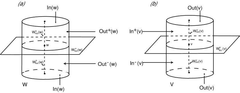
Figure 2. Cylindrical neighbourhoods of the saddle-foci ${\rm\bf w}$ (a) and ${\rm\bf v}$ (b).

In these coordinates, we consider cylindrical neighbourhoods $V$ and $W$ in ${{\rm\bf S}}^{3}$ of ${\rm\bf v}$ and ${\rm\bf w}$, respectively, of radius $\rho=\varepsilon>0$ and height $z=2\varepsilon$ — see Figure 2. After a linear rescaling of the variables, we may also assume that $\varepsilon=1$. Their boundaries consist of three components: the cylinder wall parametrised by $x\in{\rm\bf R}\pmod{2\pi}$ and $|y|\leq 1$ with the usual cover

$$(x,y)\mapsto(1,x,y)=(\rho,\theta,z)$$

and two discs, the top and bottom of the cylinder. We take polar coverings of these disks

$$(r,\varphi)\mapsto(r,\varphi,\pm 1)=(\rho,\theta,z)$$

where $0\leq r\leq 1$ and $\varphi\in{\rm\bf R}\pmod{2\pi}$. The local stable manifold of ${\rm\bf v}$, $W^{s}({\rm\bf v})$, corresponds to the circle parametrised by $y=0$. In $V$ we use the following terminology suggested in Figure 2:

• ${\text{In}}({\rm\bf v})$, the cylinder wall of $V$, consisting of points that go inside $V$ in positive time;

• ${\text{Out}}({\rm\bf v})$, the top and bottom of $V$, consisting of points that go outside $V$ in positive time.

We denote by ${\text{In}}^{+}({\rm\bf v})$ the upper part of the cylinder, parametrised by $(x,y)$, $y\in[0,1]$ and by ${\text{In}}^{-}({\rm\bf v})$ its lower part.

The cross-sections obtained for the linearisation around ${\rm\bf w}$ are dual to these. The set $W^{s}({\rm\bf w})$ is the $z$-axis intersecting the top and bottom of the cylinder $W$ at the origin of its coordinates. The set $W^{u}({\rm\bf w})$ is parametrised by $z=0$, and we use:

• ${\text{In}}({\rm\bf w})$, the top and bottom of $W$, consisting of points that go inside $W$ in positive time;

• ${\text{Out}}({\rm\bf w})$, the cylinder wall of $W$, consisting of points that go inside $W$ in negative time, with ${\text{Out}}^{+}({\rm\bf w})$ denoting its upper part, parametrised by $(x,y)$, $y\in[0,1]$ and ${\text{Out}}^{-}({\rm\bf w})$ its lower part.

We will denote by $W^{u}_{{\text{loc}}}({\rm\bf w})$ the portion of $W^{u}({\rm\bf w})$ that goes from ${\rm\bf w}$ up to ${\text{In}}({\rm\bf v})$ not intersecting the interior of $V$ and by $W^{s}_{{\text{loc}}}({\rm\bf v})$ the portion of $W^{s}({\rm\bf v})$ outside $W$ that goes directly from ${\text{Out}}({\rm\bf w})$ into ${\rm\bf v}$. The flow is transverse to these cross-sections and the boundaries of $V$ and of $W$ may be written as the closure of ${\text{In}}({\rm\bf v})\cup{\text{Out}}({\rm\bf v})$ and ${\text{In}}({\rm\bf w})\cup{\text{Out}}({\rm\bf w})$, respectively.

4.2. Local maps near the saddle-foci

Following [14, 42], the trajectory of a point $(x,y)$ with $y>0$ in ${\text{In}}({\rm\bf v})$, leaves $V$ at ${\text{Out}}({\rm\bf v})$ at

(4.2) $$\Phi_{{\rm\bf v}}(x,y)=\left(y^{\delta_{\rm\bf v}}+S_{1}(x,y;\lambda),-\frac{\ln y}{E_{\rm\bf v}}+x+S_{2}(x,y;\lambda)\right)=(r,\phi)\qquad\mbox{where}\qquad\delta_{\rm\bf v}=\frac{C_{{\rm\bf v}}}{E_{{\rm\bf v}}}>1,$$

where $S_{1}$ and $S_{2}$ are smooth functions which depend on $\lambda$ and satisfy:

(4.3) $$\left|\frac{\partial^{k+l+m}}{\partial x^{k}\partial x^{l}\partial\lambda^{m}}S_{i}(x,y;\lambda)\right|\leq Cy^{\delta_{\rm\bf v}+\sigma-l},$$

and $C$ and $\sigma$ are positive constants and $k,l,m$ are non-negative integers. Similarly, a point $(r,\phi)$ in ${\text{In}}({\rm\bf w})\backslash W^{s}_{{\text{loc}}}({\rm\bf w})$, leaves $W$ at ${\text{Out}}({\rm\bf w})$ at

(4.4) $$\Phi_{{\rm\bf w}}(r,\varphi)=\left(-\frac{\ln r}{E_{\rm\bf w}}+\varphi+R_{1}(r,\varphi;\lambda),r^{\delta_{\rm\bf w}}+R_{2}(r,\varphi;\lambda)\right)=(x,y)\qquad\mbox{where}\qquad\delta_{\rm\bf w}=\frac{C_{{\rm\bf w}}}{E_{{\rm\bf w}}}>1$$

where $R_{1}$ and $R_{2}$ satisfy a condition similar to (4.2). The terms $S_{1}$, $S_{2}$, $R_{1}$, $R_{2}$ correspond to asymptotically small terms that vanish when $y$ and $r$ go to zero. A better estimate under a stronger eigenvalue condition has been obtained in [27, Prop. 2.4].

4.3. Transition map along the connection $[{\rm\bf v}\rightarrow{\rm\bf w}]$

Points in ${\text{Out}}({\rm\bf v})$ near $W^{u}_{{\text{loc}}}({\rm\bf v})$ are mapped into ${\text{In}}({\rm\bf w})$ in a flow-box along the each one of the connections $[{\rm\bf v}\rightarrow{\rm\bf w}]$. Without loss of generality, we will assume that the transition $\Psi_{{\rm\bf v}\rightarrow{\rm\bf w}}:{\text{Out}}({\rm\bf v})\rightarrow{\text{In}}({\rm\bf w})$ does not depend on $\lambda$ and is modelled by the identity, which is compatible with hypothesis (P5). Using a more general form for $\Psi_{{\rm\bf v}\rightarrow{\rm\bf w}}$ would complicate the calculations without any change in the final results.

The coordinates on $V$ and $W$ are chosen to have $[{\rm\bf v}\rightarrow{\rm\bf w}]$ connecting points with $z>0$ in $V$ to points with $z>0$ in $W$. We will denote by $\eta$ the map $\eta=\Phi_{{\rm\bf w}}\circ\Psi_{{\rm\bf v}\rightarrow{\rm\bf w}}\circ\Phi_{{\rm\bf v}}$. Up to higher order terms, from (4.2) and (4.4), its expression in local coordinates, for $y>0$, is

(4.5) $$\eta(x,y)=\left(x-K\ln y,y^{\delta}\right)\qquad\mbox{with}\qquad\delta=\delta_{\rm\bf v}\delta_{\rm\bf w}>1\qquad\mbox{and}\qquad K=\frac{C_{\rm\bf v}+E_{\rm\bf w}}{E_{\rm\bf v}E_{\rm\bf w}}>0.$$

The choice of $\Psi_{{\rm\bf v}\rightarrow{\rm\bf w}}$ as the identity reflects the fact that the node have the same chirality. In the case where the nodes have different chirality, them map $\Psi_{{\rm\bf v}\rightarrow{\rm\bf w}}$ reverses orientation. This affects the form of the map $\eta$ and any subsequent results that use it.

4.4. Geometry of the transition map

Consider a cylinder $C$ parametrised by a covering $(\theta,y)\in{\rm\bf R}\times[-1,1]$, where $\theta$ is periodic. A helix on the cylinder $C$ accumulating on the circle $y=0$ is a curve on $C$ without self-intersections, that is the image, by the parametrisation $(\theta,y)$, of a continuous map $H:(a,b)\rightarrow{\rm\bf R}\times[-1,1]$, $H(s)=\left(H_{\theta}(s),H_{y}(s)\right)$, satisfying:

$$\lim_{s\to a^{+}}H_{\theta}(s)=\lim_{s\to b^{-}}H_{\theta}(s)=\pm\infty\qquad\lim_{s\to a^{+}}H_{y}(s)=\lim_{s\to b^{-}}H_{y}(s)=0$$

and such that there are $\tilde{a}\leq\tilde{b}\in(a,b)$ for which both $H_{\theta}(s)$ and $H_{y}(s)$ are monotonic in each of the intervals $(a,\tilde{a})$ and $(\tilde{b},b)$. It follows from the assumptions on the function $H_{\theta}$ that it has either a global minimum or a global maximum, since $\lim_{s\to a^{+}}H_{\theta}(s)=\lim_{s\to b^{-}}H_{\theta}(s)$. At the corresponding point, the projection of the helix into the circle $y=0$ is singular, a fold point of the helix. Similarly, the function $H_{y}$ always has a global maximum, that will be called the maximum height of the helix. See Figure 3.

Figure 3. A helix is defined on a covering of the cylinder by a smooth curve $(H_{\theta}(s),H_{y}(s))$ that turns around the cylinder infinitely many times as its height $H_{y}$ tends do zero. It always contains a fold point, indicated here by a diamond, and a point of maximum height, shown as a black dot.

Lemma 9.

Consider a curve on one of the cylinder walls ${\text{In}}({\rm\bf v})$ or ${\text{Out}}({\rm\bf w})$, parametrised by the graph of a smooth function $h:[a,b]\rightarrow{\rm\bf R}$, where $b-a<2\pi$ with $h(a)=h(b)=0$, $h^{\prime}(a)>0$, $h^{\prime}(b)<0$ and $h(x)>0$ for all $x\in(a,b)$. Let $M$ be the global maximum value of $h$, attained at a point $x_{M}\in(a,b)$. Then, for the transition maps defined above, we have:

1. if the curve lies in ${\text{In}}({\rm\bf v})$ then it is mapped by $\eta=\Phi_{{\rm\bf w}}\circ\Psi_{{\rm\bf v}\rightarrow{\rm\bf w}}\circ\Phi_{{\rm\bf v}}$ into a helix on ${\text{Out}}({\rm\bf w})$ accumulating on the circle ${\text{Out}}({\rm\bf w})\cap W^{u}_{{\text{loc}}}({\rm\bf w})$, its maximum height is $M^{\delta}$ and it has a fold point at $\eta(x_{*},h(x_{*}))$ for some $x_{*}\in(a,x_{M})$;

2. if the curve lies in ${\text{Out}}({\rm\bf w})$ then it is mapped by $\eta^{-1}$ into a helix on ${\text{In}}({\rm\bf v})$ accumulating on the circle ${\text{In}}({\rm\bf v})\cap W^{s}_{{\text{loc}}}({\rm\bf v})$, its maximum height is $M^{1/\delta}$ and it has a fold point at $\eta^{-1}(x_{*},h(x_{*}))$ for some $x_{*}\in(x_{M},b)$.

This result depends strongly on the form of $\eta$, and therefore, on the chirality of the nodes. If the nodes had different chirality, the graph of $h$ would no longer be mapped into a helix; the curve $\eta\left(x,h(x)\right)$ would instead have a vertical tangent at infinitely many points, see [34].

Proof.

The graph of $h$ defines a curve on ${\text{In}}({\rm\bf v})$ without self-intersections. Since $\eta$ is the transition map of a differential equation, hence a diffeomorphism, this curve is mapped by $\eta$ into a curve $H(x)=\eta\left(x,h(x)\right)=\left(H_{\theta}(x),H_{y}(x)\right)$ in ${\text{Out}}({\rm\bf w})$ without self-intersections. Using the expression (4.5) for $\eta$, we get

(4.6) $$H(x)=\left(x-K\ln h(x),\left(h(x)\right)^{\delta}\right)\qquad\text{and}\qquad H^{\prime}(x)=\left(1-\frac{Kh^{\prime}(x)}{h(x)},\delta\frac{\left(h(x)\right)^{\delta}h^{\prime}(x)}{h(x)}\right).$$

From this expression it is immediate that

$$\lim_{x\to a^{+}}H_{\theta}(x)=\lim_{x\to b^{-}}H_{\theta}(x)=+\infty\quad\text{and}\quad\lim_{x\to a^{+}}H_{y}(x)=\lim_{x\to b^{-}}H_{y}(x)=0.$$

Also,

$$H_{y}(x_{M})=M^{\delta}\geq\left(h(x)\right)^{\delta}=H_{y}(x)$$

for all $x\in\left(a,b\right)$, so the curve lies below the level $y=M^{\delta}$ in ${\text{Out}}({\rm\bf w})$. Since $h^{\prime}(b)<0$, there is an interval $(\tilde{b},b)$ where $h^{\prime}(x)<0$ and hence $H_{\theta}^{\prime}(x)>0$ and $H_{y}^{\prime}(x)<0$. Similarly, $h^{\prime}(x)>0$ on some interval $(a,\hat{a})$, where $H_{y}^{\prime}(x)>0$. For the sign of $H_{\theta}^{\prime}(x)$, note that $Kh^{\prime}(a)>0=h(a)$ and $Kh^{\prime}(x_{M})=0<h(x_{M})$. Thus, there is a point $x_{*}\in\left(a,x_{M}\right)$ where $h(x_{*})=Kh^{\prime}(x_{*})$ and $H_{\theta}^{\prime}(x)$ changes sign, this is a fold point. If $x_{*}$ is the minimum value of $x$ for which this happens, then locally the helix lies to the right of this point. This proves assertion (1). The proof of assertion  (2) is similar, using the expression

(4.7) $$\eta^{-1}(x,y)=\left(x+\frac{K}{\delta}\ln y,y^{1/\delta}\right).$$

In this case we get

$$\lim_{x\to a^{+}}H_{\theta}(x)=\lim_{x\to b^{-}}H_{\theta}(x)=-\infty$$

and if $x_{*}$ is the largest value of $x$ for which the helix has a fold point, then locally the helix lies to the left of $\eta^{-1}(x_{*},h(x_{*}))$. ∎

Note that if, instead of the graph of a smooth function, we consider continuous, positive and piecewise smooth curve $\alpha(s)$ without self-intersections from $\alpha(0)=(a,0)$ to $\alpha(1)=(b,0)$, we can apply similar arguments to show that both $\eta(\alpha)$ and $\eta^{-1}(\alpha)$ are helices.

4.5. Geometry of the invariant manifolds

There is also a well defined transition map

$$\Psi_{{\rm\bf w}\rightarrow{\rm\bf v}}^{\lambda}:{\text{Out}}({\rm\bf w})\longrightarrow{\text{In}}({\rm\bf v})$$

that depends on the $\textbf{Z}_{2}\langle\gamma_{2}\rangle$-symmetry breaking parameter $\lambda$, where $\Psi_{{\rm\bf w}\rightarrow{\rm\bf v}}^{0}$ is the identity map. We will denote by $R_{\lambda}$ the map $\Psi_{{\rm\bf w}\rightarrow{\rm\bf v}}^{\lambda}\circ\eta$, where it is well defined. When there is no risk of ambiguity, we omit the superscript $\lambda$. In this section we investigate the effect of $\Psi_{{\rm\bf w}\rightarrow{\rm\bf v}}^{\lambda}$ on the two-dimensional invariant manifolds of ${\rm\bf v}$ and ${\rm\bf w}$ for $\lambda\neq 0$, under the assumption (P7).

For this, let $f_{\lambda}$ be an unfolding of $f_{0}$ satisfying (P1)–(P7). For $\lambda\neq 0$, we introduce the notation, see Figure 4:

• $(P_{\rm\bf w}^{1},0)$ and $(P_{\rm\bf w}^{2},0)$ with $0<P_{\rm\bf w}^{1}<P_{\rm\bf w}^{2}<2\pi$ are the coordinates of the two points where the connections $[{\rm\bf w}\rightarrow{\rm\bf v}]$ of Property (P7) meet ${\text{Out}}({\rm\bf w})$;

• $(P_{\rm\bf v}^{1},0)$ and $(P_{\rm\bf v}^{2},0)$ with $0<P_{\rm\bf v}^{1}<P_{\rm\bf v}^{2}<2\pi$ are the coordinates of the two points where $[{\rm\bf w}\rightarrow{\rm\bf v}]$ meets ${\text{In}}({\rm\bf v})$;

• $(P_{\rm\bf w}^{j},0)$ and $(P_{\rm\bf v}^{j},0)$ are on the same trajectory for each $j=1,2$.

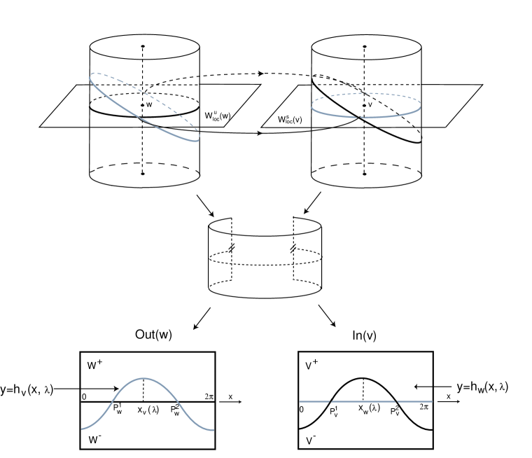
Figure 4. For $\lambda$ close to zero, $W^{s}({\rm\bf v})$ intersects the wall ${\text{Out}}({\rm\bf w})$ of the cylinder $W$ on a closed curve, given in local coordinates as the graph of a periodic function. Similarly, $W^{u}({\rm\bf w})$ meets ${\text{In}}({\rm\bf v})$ on a closed curve — this is the expected unfolding from the coincidence of the invariant manifolds at $\lambda=0$.

By (P7), for $\lambda\neq 0$, the manifolds $W^{u}({\rm\bf w})$ and $W^{s}({\rm\bf v})$ intersect transversely along the primary connections. For $\lambda$ close to zero, we are assuming that $W^{s}_{{\text{loc}}}({\rm\bf v})$ intersects the wall ${\text{Out}}({\rm\bf w})$ of the cylinder $W$ on a closed curve as in Figure 4. It corresponds to the expected unfolding from the coincidence of the manifolds $W^{s}({\rm\bf v})$ and $W^{u}({\rm\bf w})$ at $f_{0}$. Similarly, $W^{u}_{{\text{loc}}}({\rm\bf w})$ intersects the wall ${\text{In}}({\rm\bf v})$ of the cylinder $V$ on a closed curve. For small $\lambda>0$, these curves can be seen as graphs of smooth $2\pi$-periodic functions, for which we make the following conventions:

• $W^{s}_{{\text{loc}}}({\rm\bf v})\cap{\text{Out}}({\rm\bf w})$ is the graph of $y=h_{\rm\bf v}(x,\lambda)$, with $h_{\rm\bf v}(P_{\rm\bf w}^{j},\lambda)=0$, $j=1,2$;

• $W^{u}_{{\text{loc}}}({\rm\bf w})\cap{\text{In}}({\rm\bf v})$ is the graph of $y=h_{\rm\bf w}(x,\lambda)$, with $h_{\rm\bf w}(P_{\rm\bf v}^{j},\lambda)=0$, $j=1,2$;

• $h_{\rm\bf v}(x,0)\equiv 0$ and $h_{\rm\bf w}(x,0)\equiv 0$

• for $\lambda>0$, we have $h_{\rm\bf v}^{\prime}(P_{\rm\bf w}^{1},\lambda)>0$, hence $h_{\rm\bf v}^{\prime}(P_{\rm\bf w}^{2},\lambda)<0$ and $h_{\rm\bf w}^{\prime}(P_{\rm\bf v}^{1},\lambda)<0,h_{\rm\bf w}^{\prime}(P_{\rm\bf v}^{2},\lambda)>0$.

The two points $(P_{\rm\bf w}^{1},0)$ and $(P_{\rm\bf w}^{2},0)$ divide the closed curve $y=h_{\rm\bf v}(x,\lambda)$ in two components, corresponding to different signs of the second coordinate. With the conventions above, we get $h_{\rm\bf v}(x,\lambda)>0$ for $x\in\left(P_{\rm\bf w}^{1},P_{\rm\bf w}^{2}\right)$. Then the region $W^{-}$ in ${\text{Out}}({\rm\bf w})$ delimited by $W_{{\text{loc}}}^{s}({\rm\bf v})$ and $W_{{\text{loc}}}^{u}({\rm\bf w})$ between $P_{\rm\bf w}^{1}$ and $P_{\rm\bf w}^{2}$ gets mapped by $\Psi_{{\rm\bf w}\rightarrow{\rm\bf v}}^{\lambda}$ into ${\text{In}}^{-}({\rm\bf v})$, while all other points in ${\text{Out}}^{+}({\rm\bf w})$ are mapped into ${\text{In}}^{+}({\rm\bf v})$. We denote by $W^{+}$ the latter set, of points in ${\text{Out}}({\rm\bf w})$ with $0<y<1$ and $y>h_{\rm\bf v}(x,\lambda)$ for $x\in\left(P_{\rm\bf w}^{1},P_{\rm\bf w}^{2}\right)$. The maximum value of $h_{\rm\bf v}(x,\lambda)$ is attained at some point

$$(x,y)=(x_{\rm\bf v}(\lambda),M_{\rm\bf v}(\lambda))\qquad\text{with}\qquad P_{\rm\bf w}^{1}<x_{\rm\bf v}(\lambda)<P_{\rm\bf w}^{2}.$$

Finally, let $M_{\rm\bf w}(\lambda)$ be the maximum of $h_{\rm\bf w}(x,\lambda)$, attained at a point $x_{\rm\bf w}(\lambda)\in\left(P_{\rm\bf v}^{2},P_{\rm\bf v}^{1}\right)$. In order to simplify the writting, the following analysis is focused on the two Bykov cycles whose connection $[{\rm\bf v}\to{\rm\bf w}]$ lies in the subspace defined by $x_{3}\geq 0$. The same results, with minimal adaptations, hold for cycles obtained from the other connection. With this notation, we have:

Proposition 10.

Let $f_{\lambda}$ be family of vector fields satisfying (P1)–(P7). For $\lambda\neq 0$ sufficiently small, the portion of $W^{u}_{{\text{loc}}}({\rm\bf w})\cap{\text{In}}({\rm\bf v})$ that lies in ${\text{In}}^{+}({\rm\bf v})$ is mapped by $\eta$ into a helix in ${\text{Out}}({\rm\bf w})$ accumulating on $W^{u}_{{\text{loc}}}({\rm\bf w})$. If $M_{\rm\bf w}(\lambda)$ is the maximum height of $W^{u}_{{\text{loc}}}({\rm\bf w})\cap{\text{In}}^{+}({\rm\bf v})$, then the maximum height of the helix is $M_{\rm\bf w}(\lambda)^{\delta}$. For each $\lambda>0$ there is a fold point in the helix that, as $\lambda$ tends to zero, turns around the cylinder wall ${\text{Out}}({\rm\bf w})$ infinitely many times.

Proof.

That $\eta$ maps $W^{u}_{{\text{loc}}}({\rm\bf w})\cap{\text{In}}^{+}({\rm\bf v})$ into a helix, and the statement about its maximum height follow directly by applying assertion (1) of Lemma 9 to $h_{\rm\bf w}$. For the fold point in the helix, let $x_{*}(\lambda)$ be its first coordinate. From the expression (4.5) of $\eta$ it follows that

$$x_{*}(\lambda)=x_{\lambda}-K\ln h_{\rm\bf w}(x_{\lambda})$$

for some $x_{\lambda}\in(P_{\rm\bf v}^{2},x_{\rm\bf w}(\lambda))$ and with $h_{\rm\bf w}(x_{\lambda},\lambda)\leq h_{\rm\bf w}(x_{\rm\bf w}(\lambda),\lambda)=M_{\rm\bf w}(\lambda)$ and hence,

$$-K\ln h_{\rm\bf w}(x_{\lambda},\lambda)\geq-K\ln M_{\rm\bf w}(\lambda).$$

Since $f_{\lambda}$ unfolds $f_{0}$, then $\lim_{\lambda\to 0}M_{\rm\bf w}(\lambda)=0$, hence $\lim_{\lambda\to 0}-K\ln h_{\rm\bf w}(x_{\lambda},\lambda)=\infty$ and therefore, the fold point turns around the cylinder ${\text{Out}}({\rm\bf w})$ infinitely many times. ∎

The Hypothesis (P5) about chirality of the nodes is essential for Lemma 9 and Proposition 10. If we had taken the rotation in $W$ with the opposite orientation to that in $V$, the rotations would cancel out and the curve $H(x)$ defined in (4.6) would no longer be a helix, since the angular coordinate $H_{\theta}$ would not be monotonic.

5. Heteroclinic Tangencies

Using the notation and results of Section 4 we can now discuss the tangencies of the invariant manifolds and prove Theorems 4 and 5. As remarked in Section 4.5, since $f_{\lambda}$ unfolds $f_{0}$, then the maximum heights, $M_{\rm\bf v}(\lambda)$ of $W^{s}_{{\text{loc}}}({\rm\bf v})\cap{\text{Out}}({\rm\bf w})$, and $M_{\rm\bf w}(\lambda)$ of $W^{u}_{{\text{loc}}}({\rm\bf w})\cap{\text{In}}({\rm\bf v})$, satisfy:

$$\lim_{\lambda\to 0}M_{\rm\bf v}(\lambda)=\lim_{\lambda\to 0}M_{\rm\bf w}(\lambda)=0.$$

We make the additional assumption that $\left(M_{\rm\bf w}(\lambda)\right)^{\delta}$ tends to zero faster than $M_{\rm\bf v}(\lambda)$. This condition defines the open set ${\mathcal{C}}$ of unfoldings $f_{\lambda}$ that we need for the statement of Theorem 4.

The subset ${\mathcal{C}}$ of Theorem 4 is the set of families $f_{\lambda}$ of vector fields satisfying (P1)–(P7) for which there is a value $\lambda_{*}>0$ such that for $0<\lambda<\lambda_{*}$ we have $\left(M_{\rm\bf w}(\lambda)\right)^{\delta}<M_{\rm\bf v}(\lambda)$. Then ${\mathcal{C}}$ is an open subset, in the $C^{3}$ topology, of the set of families $f_{\lambda}$ of vector fields satisfying (P1)–(P7).

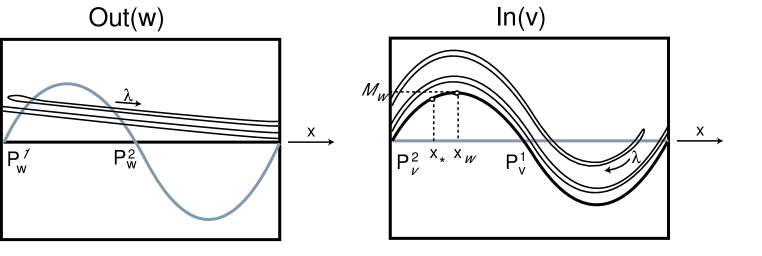
Figure 5. Left: when $\lambda$ decreases, the fold point of the helix $\alpha^{\lambda}(x)\in{\text{Out}}({\rm\bf w})$ moves to the right and for $\lambda=\lambda_{i}$ it is tangent to $W^{s}_{{\text{loc}}}({\rm\bf v})$ creating a 1-pulse tangency. Right: $\Psi_{[{\rm\bf w}\rightarrow{\rm\bf v}]}$ maps the helix $\alpha^{\lambda}(x)$ close to $W^{u}_{{\text{loc}}}({\rm\bf w})\cap{\text{In}}({\rm\bf v})$, creating several curves that satisfy the hypotheses of Lemma 9 (1). These curves are again mapped by $\eta$ into helices in ${\text{Out}}({\rm\bf w})$ creating 2-pulse heteroclinic tangencies.

5.1. Proof of Theorem 4

Suppose $f_{\lambda}\in{\mathcal{C}}$. By Proposition 10, the curve

$$\alpha^{\lambda}(x)=\eta\left(x,h_{\rm\bf w}(x,\lambda),\lambda\right)=\left(\alpha_{1}^{\lambda}(x),\alpha_{2}^{\lambda}(x)\right),\qquad x\in\left(P_{\rm\bf v}^{2},P_{\rm\bf v}^{1}\right)\pmod{2\pi}$$

is a helix in ${\text{Out}}^{+}({\rm\bf w})$ and has at least one fold point at $x=x_{*}(\lambda)$. The second coordinate of the helix satisfies $0<\alpha_{2}^{\lambda}(x)<M_{\rm\bf w}(\lambda)^{\delta}$ for all $x\in\left(P_{\rm\bf v}^{2},P_{\rm\bf v}^{1}\right)\pmod{2\pi}$ and all positive $\lambda<\lambda_{*}$. Since $f_{\lambda}\in{\mathcal{C}}$, then $\alpha_{2}^{\lambda}(x)<M_{\rm\bf v}(\lambda)$ for all $x$ and all positive $\lambda<\lambda_{*}$.

Moreover, since the fold point $\alpha^{\lambda}(x_{*}(\lambda))$ turns around ${\text{Out}}({\rm\bf w})$ infinitely many times as $\lambda$ goes to zero, given any $\lambda_{0}<\lambda_{*}$ there exists a positive value $\lambda_{R}<\lambda_{0}$ such that $\alpha^{\lambda}(x_{*}(\lambda_{R}))$ lies in $W^{+}$, the region in ${\text{Out}}({\rm\bf w})$ between $W_{{\text{loc}}}^{s}({\rm\bf v})$ and $W_{{\text{loc}}}^{u}({\rm\bf w})$ that gets mapped into the upper part of ${\text{In}}({\rm\bf v})$. Since the second coordinate of the fold point is less than the maximum of $h_{\rm\bf v}$, there is a positive value $\lambda_{L}<\lambda_{R}$ such that $\alpha^{\lambda}(x_{*}(\lambda_{L}))$ lies in $W^{-}$, the region in ${\text{Out}}({\rm\bf w})$ that gets mapped into the lower part of ${\text{In}}({\rm\bf v})$, whose boundary contains the graph of $h_{\rm\bf v}$. Therefore, the curve $\alpha^{\lambda}(x_{*}(\lambda))$ is tangent to the graph of $h_{\rm\bf v}(x,\lambda)$ at some point $\alpha(x_{*}(\lambda_{1}))$ with $\lambda_{1}\in\left(\lambda_{L},\lambda_{R}\right)$.

We have thus shown that given $\lambda_{0}>0$, there is some positive $\lambda_{1}<\lambda_{0}$, for which the image of the curve $W_{{\text{loc}}}^{u}({\rm\bf w})\cap{\text{In}}({\rm\bf v})$ by $\eta$ is tangent to $W_{{\text{loc}}}^{s}({\rm\bf v})\cap{\text{Out}}({\rm\bf w})$, creating a 1-pulse heteroclinic tangency. Two transverse 1-pulse heteroclinic connections exist for $\lambda>\lambda_{1}$ close to $\lambda_{1}$. These connections come together at the tangency and disappear.

By Proposition 10, as $\lambda$ goes to zero, the fold point $\alpha^{\lambda}(x_{*}(\lambda))$ turns around the cylinder ${\text{Out}}({\rm\bf w})$ infinitely many times, thus going in and out of $W^{-}$. Each times it crosses the boundary, a new tangency occurs. Repeating the argument above yields the sequence $\lambda_{i}$ of parameter values for which there is a 1-pulse heteroclinic tangency and this completes the proof of the main statement of Theorem 4.

On the other hand, as $\lambda$ goes to zero, the maximum height of the helix, $\left(M_{\rm\bf w}(\lambda)\right)^{\delta}$ also tends to zero. This implies that the second coordinate of the points $\alpha^{\lambda}(x_{*}(\lambda_{i}))\in{\text{Out}}({\rm\bf w})$ where there is a 1-pulse heteroclinic tangency tends to zero as $i$ goes to infinity. This shows that the tangency approaches the two-dimensional connection $[{\rm\bf w}\to{\rm\bf v}]$ that exists for $\lambda=0$.

A crucial fact in the proof of Theorem 4 is that $W^{u}_{{\text{loc}}}({\rm\bf w})\cap{\text{In}}({\rm\bf v})$ is the graph of a function with a single maximum, and that this maximum goes to 0 as $\lambda$ goes to 0. This follows because the family $f_{\lambda}$ unfolds the more symmetric vector field $f_{0}$. We could make the assumption on the invariant manifold directly, but it is the context of symmetry-breaking that makes it natural.

The construction in the proof of Theorem 4 may be extended to obtain multipulse tangencies, as follows:

5.2. Proof of Theorem 5

Look at $W^{u}_{{\text{loc}}}({\rm\bf w})\cap{\text{In}}({\rm\bf v})$, the graph of $h_{\rm\bf w}(x,\lambda)$. Since $h_{\rm\bf w}^{\prime}(P_{\rm\bf v}^{1},\lambda)<0$, there is an interval $[\tilde{x},P_{\rm\bf v}^{1}]\subset[x_{\rm\bf w}(\lambda),P_{\rm\bf v}^{1}]$ where the map $h_{\rm\bf w}$ is monotonically decreasing. Note that the hypothesis of different chirality is essential here. Therefore, we may define infinitely many intervals where $\alpha^{\lambda}(x)=\eta\left(x,h_{\rm\bf w}(x,\lambda)\right)$ lies in $W^{+}$. More precisely, we have two sequences, $(a_{j})$ and $(b_{j})$ in $[\tilde{x},P_{\rm\bf v}^{1}]$ such that:

• $a_{j}<b_{j}<a_{j+1}$ with  $\lim_{j\to\infty}a_{j}=P_{\rm\bf v}^{1}$;

• $\alpha^{\lambda}(a_{j})$ and $\alpha^{\lambda}(b_{j})\in W^{s}_{loc}({\rm\bf v})\cap{\text{Out}}^{+}({\rm\bf w})$;

• if $x\in(a_{j},b_{j})$ then $\alpha^{\lambda}(x)\in W^{+}$;

• the curves $\alpha^{\lambda}\left([a_{j},b_{j}]\right)$ accumulate uniformly on $W^{u}_{{\text{loc}}}({\rm\bf w})\cap{\text{Out}}({\rm\bf w})$ as $j\to\infty$.

Hence, each one of the curves $\alpha^{\lambda}\left([a_{j},b_{j}]\right)$ is mapped by $\Psi_{{\rm\bf w}\rightarrow{\rm\bf v}}$ into the graph of a function $h$ in ${\text{In}}({\rm\bf v})$ satisfying the conditions of Lemma 9, and hence each one of these curves is mapped by $\eta$ into a helix $\xi_{j}(x)$, $x\in(a_{j},b_{j})$.

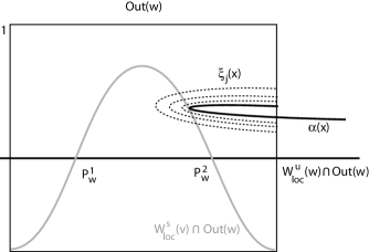
Figure 6. Curves in the proof of Theorem 5: for $\lambda=\lambda_{i}$ the curve $\alpha^{\lambda}(x)=\eta(W^{u}_{{\text{loc}}}({\rm\bf w})\cap{\text{In}}^{+}({\rm\bf v}))$ (solid black curve) is tangent to $W^{s}_{{\text{loc}}}({\rm\bf v})$ (gray curve) in ${\text{Out}}({\rm\bf w})$. The curves $\xi_{j}(x)$ (dotted) accumulate on $\alpha^{\lambda}(x)$. Very small changes in $\lambda$ make them tangent to $W^{s}_{{\text{loc}}}({\rm\bf v})$ creating 2-pulse heteroclinic tangencies.

Let $\lambda_{i}$ be a parameter value for which $\dot{x}=f_{\lambda_{i}}(x)$ has a 1-pulse heteroclinic tangency as stated in Theorem 4. As $j\rightarrow+\infty$, the helices $\xi_{j}(x)$ accumulate on the helix of Theorem 4 as drawn in Figure 6, hence the fold point of $\xi_{j}(x)$ is arbitrarily close to the fold point of $\eta(x,h_{\rm\bf w}(x,\lambda))$. The arguments in the proof of Theorem 4 show that a small change in the parameter $\lambda$ makes the new helix tangent to $W^{s}_{{\text{loc}}}({\rm\bf v})$ as in Figure 5. For each $j$ this creates a 2-pulse heteroclinic tangency at $\lambda=\lambda_{ij}$. Since the the helices $\xi_{j}(x)$ accumulate on $\alpha^{\lambda_{i}}(x)$, it follows that $\lim_{j\in{\rm\bf N}}\lambda_{ij}=\lambda_{i}$.

Finally, the argument may be applied recursively to show that each $n$-pulse heteroclinic tangency is accumulated by $(n+1)$-pulse heteroclinic tangencies for nearby parameter values.

If $\lambda^{\star}\in{\rm\bf R}$ is such that the flow of $\dot{x}=f_{\lambda^{\star}}(x)$ has a heteroclinic tangency, when $\lambda$ varies near $\lambda^{\star}$, we find the creation and the destruction of horseshoes that is accompanied by Newhouse phenomena [22, 54]. In terms of numerics, we know very little about the geometry of these attractors, we also do not know the size and the shape of their basins of attraction. Basin boundary metamorphoses and explosions of chaotic saddles as those described in [45] are expected.

6. Bifurcating dynamics

We discuss here the geometric constructions that determine the global dynamics near a Bykov cycle, in order to prove Theorem 6. For this we need some preliminary definitions and more information on the geometry of the transition maps. First, we adapt the definition of horizontal strip in [26] to serve our purposes: for $\tau>0$ sufficiently small, in the local coordinates of the walls of the cylinders $V$ and $W$, consider the rectangles:

$${\mathcal{S}}_{\rm\bf v}=[P_{\rm\bf v}^{2}-\tau,P_{\rm\bf v}^{1}+\tau]\times[0,1]\subset{\text{In}}({\rm\bf v})\qquad\text{and}\qquad{\mathcal{S}}_{\rm\bf w}=[P_{\rm\bf w}^{2}-\tau,P_{\rm\bf w}^{1}+\tau]\times[0,1]\subset{\text{Out}}({\rm\bf w})$$

with the conventions $-\pi<P_{\rm\bf v}^{2}-\tau<P_{\rm\bf v}^{1}+\tau\leq\pi$ and $-\pi<P_{\rm\bf w}^{2}-\tau<P_{\rm\bf w}^{1}+\tau\leq\pi$.

A horizontal strip in ${\mathcal{S}}_{\rm\bf v}$ is a subset of ${\text{In}}^{+}({\rm\bf v})$ of the form

$${\mathcal{H}}=\left\{(x,y)\in In^{+}({\rm\bf v}):\quad x\in[P_{\rm\bf v}^{2}-\tau,P_{\rm\bf v}^{1}+\tau]\qquad\text{and}\quad y\in[u_{1}(x),u_{2}(x)]\right\},$$

where $u_{1},u_{2}:[P_{\rm\bf v}^{2}-\tau,P_{\rm\bf v}^{1}+\tau]\rightarrow(0,1]$ are smooth maps such that $u_{1}(x)<u_{2}(x)$ for all $x\in[P_{\rm\bf v}^{2}-\tau,P_{\rm\bf v}^{1}+\tau]$. The graphs of the $u_{j}$ are called the horizontal boundaries of ${\mathcal{H}}$ and the segments $\left(P_{\rm\bf v}^{2}-\tau,y\right)$, $u_{1}(P_{\rm\bf v}^{2}-\tau)\leq y\leq u_{2}(P_{\rm\bf v}^{2}-\tau)$ and $\left(P_{\rm\bf v}^{1}+\tau,y\right)$, with $u_{1}(P_{\rm\bf v}^{1}+\tau)\leq y\leq u_{2}(P_{\rm\bf v}^{1}+\tau)$ are its vertical boundaries. Horizontal and vertical boundaries intersect at four vertices. The maximum height and the minimum height of ${\mathcal{H}}$ are, respectively

$$\max_{x\in[P_{\rm\bf v}^{2}-\tau,P_{\rm\bf v}^{1}+\tau]}u_{2}(x)\qquad\qquad\min_{x\in[P_{\rm\bf v}^{2}-\tau,P_{\rm\bf v}^{1}+\tau]}u_{1}(x).$$

Analogously we may define a horizontal strip in ${\mathcal{S}}_{\rm\bf w}\subset{\text{Out}}^{+}({\rm\bf w})$.

A horseshoe strip in ${\mathcal{S}}_{\rm\bf v}$ is a subset of ${\text{In}}^{+}({\rm\bf v})$ of the form

$$\left\{(x,y)\in{\text{In}}^{+}({\rm\bf v}):\quad x\in[a_{2},b_{2}],\quad y\in[u_{1}(x),u_{2}(x)]\right\},$$

where

• $[a_{1},b_{1}]\subset[a_{2},b_{2}]\subset[P_{\rm\bf v}^{2}-\tau,P_{\rm\bf v}^{1}+\tau]$;

• $u_{1}(a_{1})=u_{1}(b_{1})=0$;

• $u_{2}(a_{2})=u_{2}(b_{2})=0$.

The boundary of ${\mathcal{H}}$ consists of the graph of $u_{2}(x)$, $x\in[a_{2},b_{2}]$, the graph of $u_{1}(x)$, $x\in[a_{1},b_{1}]$, together with the two pieces of $W^{s}_{{\text{loc}}}({\rm\bf v})\cap{\text{In}}({\rm\bf v})$ with $x\in[a_{2},a_{1}]$ and $x\in[b_{1},b_{2}]$.

6.1. Horseshoe strips in ${\mathcal{S}}_{\rm\bf v}$

We are interested in the dynamics of points whose trajectories start in ${\mathcal{S}}_{\rm\bf v}$ and return to ${\text{In}}^{+}({\rm\bf v})$ arriving at ${\mathcal{S}}_{\rm\bf v}$.

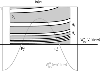
Figure 7. For $\lambda>0$ sufficiently small, the set $\eta^{-1}({\mathcal{S}}_{\rm\bf w})\cap{\mathcal{S}}_{\rm\bf v}$ has infinitely many connected components (gray region), all of which, except maybe for the top ones, define horizontal strips in ${\mathcal{S}}_{\rm\bf v}$ accumulating on $W^{s}_{loc}({\rm\bf v})\cap{\text{In}}({\rm\bf v})$ (gray curve).

Lemma 11.

The set $\eta^{-1}({\mathcal{S}}_{\rm\bf w})\cap{\mathcal{S}}_{\rm\bf v}$ has infinitely many connected components all of which are horizontal strips in ${\mathcal{S}}_{\rm\bf v}$ accumulating on $W^{s}_{{\text{loc}}}({\rm\bf v})\cap{\text{In}}({\rm\bf v})$, except maybe for a finite number. The horizontal boundaries of these strips are graphs of monotonically increasing functions of $x$.

Proof.

The boundary of ${\mathcal{S}}_{\rm\bf w}$ consists of the following:

1. a piece of $W^{u}_{{\text{loc}}}({\rm\bf w})\cap{\text{Out}}({\rm\bf w})$ parametrised by $y=0$, $x\in[P^{1}_{\rm\bf w}-\tau,P^{2}_{\rm\bf w}+\tau]$, where $\eta^{-1}$ is not defined;

2. the horizontal segment $(x,1)$ with $x\in[P_{\rm\bf w}^{2}-\tau,P_{\rm\bf w}^{1}+\tau]$;

3. two vertical segments $\left(P^{1}_{\rm\bf w}-\tau,y\right)$ and $\left(P^{2}_{\rm\bf w}+\tau,y\right)$ with $y\in\left(0,1\right)$.

Together, the components (2) and (3) form a continuous curve that, by the arguments of Lemma 9 (2), is mapped by $\eta$ into a helix on ${\text{In}}^{+}({\rm\bf v})$, accumulating on $W^{s}_{{\text{loc}}}({\rm\bf v})\cap{\text{In}}({\rm\bf v})$. As the helix approaches $W^{s}_{{\text{loc}}}({\rm\bf v})$, it crosses the vertical boundaries of ${\mathcal{S}}_{\rm\bf v}$ infinitely many times. The interior of ${\mathcal{S}}_{\rm\bf w}$ is mapped into the space between consecutive crossings, intersecting ${\mathcal{S}}_{\rm\bf v}$ in horizontal strips, as shown in Figure 7. From the expression (4.7) of $\eta^{-1}$ it also follows that the vertical boundaries of ${\mathcal{S}}_{\rm\bf w}$ are mapped into graphs of monotonically increasing functions of $x$. ∎

Here, as in the next two Lemmas, we are using the form of the map $\eta$ through Lemma 9, hence the result depends strongly on the chirality hypothesis (P5).

Denote by ${\mathcal{H}}_{n}$ the strip that attains its maximum height $h_{n}$ at the vertex $\left(P^{1}_{\rm\bf v}+\tau,h_{n}\right)$ with

(6.8) $$h_{n}={\rm e}^{(P^{1}_{\rm\bf v}-P^{2}_{\rm\bf w}+2\tau-2n\pi)/K},$$

then $\lim_{n\to\infty}h_{n}=0$, hence the strips ${\mathcal{H}}_{n}$ accumulate on $W^{s}_{{\text{loc}}}({\rm\bf v})\cap{\text{In}}({\rm\bf v})$. The minimum height of ${\mathcal{H}}_{n}$ is given by

(6.9) $$m_{n}={\rm e}^{(P^{2}_{\rm\bf v}-P^{1}_{\rm\bf w}-2\tau-2n\pi)/K}$$

and is attained at the vertex $\left(P^{2}_{\rm\bf v}-\tau,m_{n}\right)$. Moreover $n<m$ implies that ${\mathcal{H}}_{n}$ lies above ${\mathcal{H}}_{m}$.

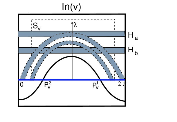
Figure 8. Horseshoe strips: for $\lambda>0$ sufficiently small, the set $R_{\lambda}(\eta^{-1}({\mathcal{S}}_{\rm\bf w})\cap{\mathcal{S}}_{\rm\bf v})\subset{\text{In}}^{+}({\rm\bf v})$ defines a countably infinite number of horseshoe strips in ${\mathcal{S}}_{\rm\bf v}$, that accumulate on $W^{u}_{{\text{loc}}}({\rm\bf w})\cap{\text{In}}({\rm\bf v})$.

Lemma 12.

Let ${\mathcal{H}}_{n}$ be one of the horizontal strips in $\eta^{-1}({\mathcal{S}}_{\rm\bf w})\cap{\mathcal{S}}_{\rm\bf v}$. Then $\eta({\mathcal{H}}_{n})$ is a horizontal strip in ${\mathcal{S}}_{\rm\bf w}$. The strips $\eta({\mathcal{H}}_{n})$ accumulate on $W^{u}_{{\text{loc}}}({\rm\bf w})\cap{\text{In}}({\rm\bf v})$ as $n\to\infty$ and the maximum height of $\eta({\mathcal{H}}_{n})$ is $h_{n}^{\delta}$, where $h_{n}$ is the maximum height of ${\mathcal{H}}_{n}$.

Proof.

The boundary of ${\mathcal{S}}_{\rm\bf v}$ consists of a piece of $W^{s}_{{\text{loc}}}({\rm\bf v})$ plus a curve formed by three segments, two of which are vertical and a horizontal one. From the arguments of Lemma 9 (1), it follows that the part of the boundary of ${\mathcal{S}}_{\rm\bf v}$ not contained in $W^{s}_{{\text{loc}}}({\rm\bf v})$ is mapped by $\eta$ into a helix.

Consider now the effect of $\eta$ on the boundary of ${\mathcal{H}}_{n}$. Each horizontal boundary gets mapped into a piece of one of the vertical boundaries of ${\mathcal{S}}_{\rm\bf w}$. The vertical boundaries of ${\mathcal{H}}_{n}$ are contained in those of ${\mathcal{S}}_{\rm\bf v}$ and hence are mapped into two pieces of a helix, that will form the horizontal boundaries of the strip $\eta({\mathcal{H}}_{n})$, that may be written as graphs of decreasing functions of $x$.

A shown after Lemma 11, the maximum height of ${\mathcal{H}}_{n}$ tends to zero, hence the strips $\eta({\mathcal{H}}_{n})$ have the same property. The maximum height of $\eta({\mathcal{H}}_{n})$ is $h_{n}^{\delta}$, attained at the point $\left(P^{2}_{\rm\bf w}-\tau,h_{n}^{\delta}\right)$. ∎

Lemma 13.

For each $\lambda>0$ sufficiently small, there exists $n_{0}(\lambda)$ such that for all $n\geq n_{0}$ the image $R_{\lambda}({\mathcal{H}}_{n})$ of the horizontal strips in $\eta^{-1}({\mathcal{S}}_{\rm\bf w})\cap{\mathcal{S}}_{\rm\bf v}$ intersects ${\mathcal{S}}_{\rm\bf v}$ in a horseshoe strip. The strips $R_{\lambda}({\mathcal{H}}_{n})$ accumulate on $W^{u}_{{\text{loc}}}({\rm\bf w})\cap{\text{In}}({\rm\bf v})$ and, when $n\to\infty$, their maximum height tends to $M_{\rm\bf w}(\lambda)$, the maximum height of $W^{u}_{{\text{loc}}}({\rm\bf w})\cap{\text{In}}({\rm\bf v})$.

Proof.

The curve $W^{s}_{{\text{loc}}}({\rm\bf v})\cap{\text{Out}}({\rm\bf w})$ is the graph of the function $h_{\rm\bf v}(x,\lambda)$ that is positive for $x$ outside the interval $[P^{2}_{\rm\bf w},P^{1}_{\rm\bf w}]\pmod{2\pi}$. In particular, $h_{\rm\bf v}(P^{2}_{\rm\bf w}-\tau,\lambda)>0$ and $h_{\rm\bf v}(P^{2}_{\rm\bf w}+\tau,\lambda)>0$ for small $\tau>0$. Therefore there is a piece of the vertical boundary of ${\mathcal{S}}_{\rm\bf w}$ that lies below $W^{s}_{{\text{loc}}}({\rm\bf v})\cap{\text{Out}}({\rm\bf w})$, consisting of the two segments $(P^{2}_{\rm\bf w}-\tau,y)$ with $0<y<h_{\rm\bf v}(P^{2}_{\rm\bf w}-\tau,\lambda)$ and $(P^{1}_{\rm\bf w}+\tau,y)$ with $0<y<h_{\rm\bf v}(P^{1}_{\rm\bf w}+\tau,\lambda)$. For small $\lambda>0$, these segments are mapped by $\Psi_{{\rm\bf w}\to{\rm\bf v}}^{\lambda}$ inside ${\text{In}}^{-}({\rm\bf v})$.

Let $n_{0}$ be such that the maximum height of $\eta({\mathcal{H}}_{n_{0}})$ is less than the minimum of

$$h_{\rm\bf v}(P^{2}_{\rm\bf w}-\tau,\lambda)>0\qquad\text{and}\qquad h_{\rm\bf v}(P^{2}_{\rm\bf w}+\tau,\lambda)>0.$$

Then for any $n\geq n_{0}$ the vertical sides of $\eta({\mathcal{H}}_{n})$ are mapped by $\Psi_{{\rm\bf w}\to{\rm\bf v}}^{\lambda}$ inside ${\text{In}}^{-}({\rm\bf v})$. The horizontal boundaries of $\eta({\mathcal{H}}_{n})$ go across ${\mathcal{S}}_{\rm\bf w}$, so writing them them as graphs of $u_{1}(x)<u_{2}(x)$, there is an interval where the second coordinate of $\Psi_{{\rm\bf w}\to{\rm\bf v}}^{\lambda}(x,u_{j}(x))$ is more than $M_{\rm\bf w}(\lambda)>0$, the maximum height of $W^{u}_{{\text{loc}}}({\rm\bf w})\cap{\text{In}}^{+}({\rm\bf v})$. Since the second coordinate of $\Psi_{{\rm\bf w}\to{\rm\bf v}}^{\lambda}(x,u_{j}(x))$ changes sign twice, then it equals zero at two points, hence $R_{\lambda}({\mathcal{H}}_{n})\cap{\mathcal{S}}_{\rm\bf v}$ is a horseshoe strip.

We have shown that the maximum height of $\eta({\mathcal{H}}_{n})$ tends to zero as $n\to\infty$, hence the maximum height of $R_{\lambda}({\mathcal{H}}_{n})=\Psi_{{\rm\bf w}\to{\rm\bf v}}^{\lambda}(\eta({\mathcal{H}}_{n}))$ tends to $M_{\rm\bf w}(\lambda)$. ∎

6.2. Regular Intersections of Strips

We now discuss the global dynamics near the Bykov cycle. The structure of the non-wandering set near the network depends on the geometric properties of the intersection of ${\mathcal{H}}_{n}$ and $R_{\lambda}({\mathcal{H}}_{n})$.

Let $A$ be a horseshoe strip and $B$ be a horizontal strip in ${\mathcal{S}}_{\rm\bf v}$. We say that $A$ and $B$ intersect regularly if $A\cap B\neq\emptyset$ and each one of the horizontal boundaries of $A$ goes across each one of the horizontal boundaries of $B$. Intersections that are neither empty nor regular, will be called irregular.

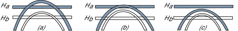
Figure 9. Strips in Proposition 15: (a) $\lambda=\lambda_{3}$; (b) $\lambda=\lambda_{2}$; (c) $\lambda=\lambda_{1}$. The position of the horizontal strips ${\mathcal{H}}_{a}$ and ${\mathcal{H}}_{b}$ does not depend on $\lambda$. The maximum height of the horseshoe strips $R_{\lambda}({\mathcal{H}}_{a})$ and $R_{\lambda}({\mathcal{H}}_{b})$ decreases when $\lambda$ decreases, and the suspended horseshoe in $R_{\lambda}({\mathcal{H}}_{a})\cap{\mathcal{H}}_{a}$ is destroyed.

If the horseshoe strip $A$ and the horizontal strip $B$ intersect regularly, then $A\cap B$ has at least two connected components, see Figure 8. In this and the next subsection, we will find that the horizontal strips ${\mathcal{H}}_{n}$ across ${\mathcal{S}}_{\rm\bf v}$ may intersect $R_{\lambda}({\mathcal{H}}_{m})$ in the three ways: empty, regular and irregular, but there is an ordering for the type of intersection, as shown in Figure 9.

Lemma 14.

For any given fixed $\lambda>0$ sufficiently small, there exists $N(\lambda)\in{\rm\bf N}$ such that for all $m,n>N(\lambda)$, the horseshoe strips $R_{\lambda}({\mathcal{H}}_{m})$ in ${\mathcal{S}}_{\rm\bf v}$ intersect each one of the horizontal strips ${\mathcal{H}}_{n}$ regularly.

Proof.

From Lemma 13 we obtain $n_{0}(\lambda)$ such that all $R_{\lambda}({\mathcal{H}}_{m})$ with $m\geq n_{0}(\lambda)$ are horseshoe strips and their lower horizontal boundary has maximum height bigger than the maximum height $M_{\rm\bf w}(\lambda)$ of $W^{u}_{{\text{loc}}}({\rm\bf w})\cap{\text{In}}({\rm\bf v})$.

On the other hand, since the strips ${\mathcal{H}}_{n}$ accumulate uniformly on $W^{s}_{{\text{loc}}}({\rm\bf v})\cap{\text{In}}({\rm\bf v})$, with their maximum height $h_{n}$ tending to zero, then there exists $n_{1}(\lambda)$ such that $h_{n}<M_{\rm\bf w}(\lambda)$ for all $n\geq n_{1}(\lambda)$. Note that the $h_{n}$ do not depend on $\lambda$. Therefore, for $m,n>N(\lambda)=\max\{n_{0}(\lambda),n_{1}(\lambda)\}$ both horizontal boundaries of $R_{\lambda}({\mathcal{H}}_{m})$ go across the two horizontal boundaries of ${\mathcal{H}}_{n}$. ∎

The constructions of this section also hold for the backwards return map $R^{-1}$ with analogues to Lemmas 11, 12, 13 and 14.

Generically, for $n>N(\lambda)$ each horizontal strip ${\mathcal{H}}_{n}$ intersects $R_{\lambda}({\mathcal{H}}_{n})$ in two connected components. Thus the dynamics of points whose trajectories always return to ${\text{In}}({\rm\bf v})$ in ${\mathcal{H}}_{n}$ may be coded by a full shift on two symbols, that describe which component is visited by the trajectory on each return to ${\mathcal{H}}_{n}$. Similarly, trajectories that return to ${\mathcal{S}}_{\rm\bf v}$ inside ${\mathcal{H}}_{n}\cup\cdots\cup{\mathcal{H}}_{n+k}$ may be coded by a full shift on $2k$ symbols. As $k\to\infty$, the strips ${\mathcal{H}}_{n+k}$ approach $W^{s}_{{\text{loc}}}({\rm\bf v})\cap{\text{In}}({\rm\bf v})$ and the number of symbols tends to infinity. We have recovered the horseshoe dynamics described in assertion (4) of Theorem 2.

The regular intersection of Lemma 14 implies the existence of an $R_{\lambda}$-invariant subset in $\eta^{-1}({\mathcal{S}}_{\rm\bf w})\cap{\mathcal{S}}_{\rm\bf v}$, the Cantor set of initial conditions:

$$\Lambda=\bigcap_{j\in{\rm\bf Z}}\bigcup_{m,n\geq N(\lambda)}\left({R_{\lambda}}^{j}({\mathcal{H}}_{m})\cap{\mathcal{H}}_{n}\right),$$

where the return map to $\eta^{-1}({\mathcal{S}}_{\rm\bf w})\cap{\mathcal{S}}_{\rm\bf v}$ is well defined in forward and backward time, for arbitrarily large times. We have shown here that the map $R_{\lambda}$ restricted to this set is semi-conjugate to a full shift over a countable alphabet. Results of [3, 34] show that the first return map is hyperbolic in each horizontal strip, implying the full conjugacy to a shift. The time of return of points in ${\mathcal{H}}_{j}$ tends to $+\infty$, as $j\to+\infty$. The set $\Lambda$ depends strongly on the parameter $\lambda$, in the next subsection we discuss its bifurcations when $\lambda$ decreases to zero.

6.3. Irregular intersections of strips

The horizontal strips ${\mathcal{H}}_{n}$ that comprise $\eta^{-1}({\mathcal{S}}_{\rm\bf w})\cap{\mathcal{S}}_{\rm\bf v}$ do not depend on the bifurcation parameter $\lambda$, as shown in Lemmas 11 and 12. This is in contrast with the strong dependence on $\lambda$ shown by the first return of these points to ${\mathcal{S}}_{\rm\bf v}$ at the horseshoe strips $R_{\lambda}({\mathcal{H}}_{n})$. In particular, the values of $n_{0}(\lambda)$ (Lemma 13) and $N(\lambda)$ (Lemma 14) vary with the choice of $\lambda$. For a small fixed $\lambda>0$ and for $m,n\geq N(\lambda)$ we have shown that ${\mathcal{H}}_{n}$ and $R_{\lambda}({\mathcal{H}}_{m})$ intersect regularly.

The next result describes the bifurcations of these sets when $\lambda$ decreases. These global bifurcations have been described by Palis and Takens in [43] in a different context, where the horseshoe strips are translated down as a parameter varies. In our case, when $\lambda$ goes to zero the horseshoe strips are flattened into the common invariant two-dimensional manifoldsof ${\rm\bf v}$ and ${\rm\bf w}$.

Proposition 15.

Given $\lambda_{3}>0$ sufficiently small, there exist $\lambda_{1}<\lambda_{2}<\lambda_{3}\in{\rm\bf R}^{+}$, a horizontal strip ${\mathcal{H}}_{a}$ across ${\mathcal{S}}_{\rm\bf v}\subset{\text{In}}^{+}({\rm\bf v})$ and $b_{0}>a$ such that for any $b>b_{0}$ the horizontal strips ${\mathcal{H}}_{a}$ and ${\mathcal{H}}_{b}$ satisfy:

1. for $\lambda=\lambda_{3}$ the sets ${\mathcal{H}}_{i}$ and $R_{\lambda_{3}}({\mathcal{H}}_{j})$ intersect regularly for $i,j\in\{a,b\}$;

2. for $\lambda=\lambda_{2}$ the intersection ${\mathcal{H}}_{a}\cap R_{\lambda_{2}}({\mathcal{H}}_{a})$ is irregular;

3. for $\lambda=\lambda_{1}$ the sets ${\mathcal{H}}_{a}$ and $R_{\lambda_{1}}({\mathcal{H}}_{a})$ do not intersect at al;

4. for $\lambda=\lambda_{1}$ and $\lambda=\lambda_{2}$ the set $R_{\lambda}({\mathcal{H}}_{b})$ intersects both ${\mathcal{H}}_{b}$ and ${\mathcal{H}}_{a}$ regularly.

Proof.

As we have remarked before, the horizontal strips ${\mathcal{H}}_{n}$ do not depend on the parameter $\lambda$. In particular, they are well defined for $\lambda=0$. Their image by the return map $R_{0}$ is no longer a horseshoe strip, it is a horizontal strip across ${\mathcal{S}}_{\rm\bf v}$. Since for $\lambda=0$ the map $\Psi_{{\rm\bf w}\rightarrow{\rm\bf v}}^{0}$ is the identity (see 4.5) and the network is asymptotically stable, it follows that the maximum height of $R_{0}({\mathcal{H}}_{n})$ is no more than that of $\eta({\mathcal{H}}_{n})$.

From Lemma 12 and the expressions (6.8) and (6.9) for the maximum, $h_{n}$, and minimum $m_{n}$, height of ${\mathcal{H}}_{n}$, we get that the maximum height $h_{n}^{\delta}$ of $\eta({\mathcal{H}}_{n})$ is less than $m_{n}$ if

$$L_{n}=\delta(P^{1}_{\rm\bf v}-P^{2}_{\rm\bf w})+2\tau(\delta-1)-2n\pi(\delta-1)<P^{2}_{\rm\bf v}-P^{1}_{\rm\bf w}.$$

Since $\lim_{n\to\infty}L_{n}=-\infty$, there is $n_{2}$ such that $R_{0}({\mathcal{H}}_{n})\cap{\mathcal{H}}_{n}=\emptyset$, for every $n>n_{2}$. Therefore, since $R_{\lambda}$ is continuous on $\lambda$, for each $n>n_{2}$ there is $\lambda_{\star}(n)>0$ such that the maximum height of $R_{\lambda(n)}({\mathcal{H}}_{n})$ is less than that of ${\mathcal{H}}_{n}$.

Let $a=\max\{n_{1},N(\lambda_{3})\}$ for $N(\lambda_{3})$ from Lemma 14. Then assertion (1) is true for this ${\mathcal{H}}_{a}$ and for any ${\mathcal{H}}_{n}$ with $n>a$, by Lemma 14. We obtain assertion (3) by taking $\lambda_{1}=\lambda_{\star}(a)$. Assertion (2) follows from the continuous dependence of $R_{\lambda}$ on $\lambda$. Assertion (4) holds for any ${\mathcal{H}}_{b}$ with $b>N(\lambda_{1})=b_{0}$ by Lemma 14. ∎

6.4. Proof of Theorem 6

In particular, Proposition 15 implies that there exists $d\in[\lambda_{2},\lambda_{3})$ such that at $\lambda=d$, the lower horizontal boundary of $R_{\lambda}({\mathcal{H}}_{a})$ is tangent to the upper horizontal boundary of ${\mathcal{H}}_{a}$. Analogously, there exists $c\in(\lambda_{1},\lambda_{2}]$ such that at $\lambda=c$, the upper horizontal boundary of $R_{\lambda}({\mathcal{H}}_{a})$ is tangent to the lower horizontal boundary of ${\mathcal{H}}_{a}$. There are infinitely many values of $\lambda$ in $[c,d]$ for which the map $R_{\lambda}$ has a homoclinic tangency associated to a periodic point see [43, 54].

The rigorous formulation of Theorem 6 consists of Proposition 15 , with $\Delta_{1}=[c,d]$ as in the remarks above. Since Proposition 15 holds for any $\lambda_{3}>0$, it may be applied again with $\lambda_{3}$ replaced by $\lambda_{1}$, and the argument may be repeated recursively to obtain a sequence of disjoint intervals $\Delta_{n}$.

6.5. Proof of Corollary 7

The $\lambda$ dependence of the position of the horseshoe strips is not a translation in our case, but after Proposition 15 the constructions of Yorke and Alligood [54] and of Palis and Takens [43] can be carried over. Hence, when the parameter $\lambda$ varies between two consecutive regular intersections of strips, the bifurcations of the first return map can be described as the one-dimensional parabola-type map in [43]. Following [43, 54], the bifurcations for $\lambda\in[\lambda_{1},\lambda_{3}]$ are:

• for $\lambda>d$: the restriction of the map $R_{\lambda_{3}}$ to the non-wandering set on ${\mathcal{H}}_{a}$ is conjugate to the Bernoulli shift of two symbols and it no longer bifurcates as $\lambda$ increases.

• at $\lambda\in(c,d)$: a fixed point with multiplier equal to $\pm 1$ appears at a tangency of the horizontal boundaries. It undergoes a period-doubling bifurcation. A cascade of period-doubling bifurcations leads to chaotic dynamics which alternates with stability windows and the bifurcations stop at $\lambda=d$;

• at $\lambda<c$: trajectories with initial conditions in ${\mathcal{H}}_{a}$ approach the network and might be attracted to another basic set.

6.6. Proof of Corollary 8

If the first return map $R_{\lambda}$ is area-contracting, then the fixed point that appears for $\lambda\in(c,d)$ is attracting for the parameter in an open interval.

This attracting fixed point bifurcates to a sink of period 2 at a bifurcation parameter $\lambda>c$ close to $c$. This stable orbit undergoes a second flip bifurcation, yielding an orbit of period 4. This process continues to an accumulation point in parameter space at which attracting orbits of period $2^{k}$ exist, for all $k\in{\rm\bf N}$. This completes the proof of Corollary 8 .

Finally, we describe a setting in which the fixed point that appears for $\lambda\in(c,d)$ can be shown to be attracting. Recall that the set $W^{u}_{{\text{loc}}}({\rm\bf w})\cap{\text{In}}({\rm\bf v})$ is the graph of $y=h_{\rm\bf w}(x,\lambda)$. Suppose the transition map $\Psi_{{\rm\bf w}\rightarrow{\rm\bf v}}^{\lambda}:{\text{Out}}({\rm\bf w})\longrightarrow{\text{In}}({\rm\bf v})$ is given by $\Psi_{{\rm\bf w}\rightarrow{\rm\bf v}}^{\lambda}(x,y)=\left(x,y+h_{\rm\bf w}(x,\lambda)\right)$, which is consistent with Section  4.5. Since

$$D\Psi_{{\rm\bf w}\rightarrow{\rm\bf v}}^{\lambda}(x,y)=\left(\begin{array}[]{cc}1&0\\ \frac{\partial h_{\rm\bf w}}{\partial x}(x)&1\end{array}\right)\quad\mbox{and}\quad D\eta(x,y)=\left(\begin{array}[]{cc}1&\displaystyle\frac{-K}{y}\\ \\ 0&\delta y^{\delta-1}\end{array}\right)$$

then

$$\det DR_{\lambda}(x,y)=\det D\Psi_{{\rm\bf w}\rightarrow{\rm\bf v}}^{\lambda}\left(\eta(x,y)\right)\cdot\det D\eta(x,y)=\delta y^{\delta-1}.$$

For sufficiently small $y$ (in ${\mathcal{H}}_{n}$ with sufficiently large $n$) this is less than 1, and hence $R_{\lambda}$ is contracting. However, if the first coordinate of $\Psi_{{\rm\bf w}\rightarrow{\rm\bf v}}^{\lambda}(x,y)$ depends on $y$, then $\det D\Psi_{{\rm\bf w}\rightarrow{\rm\bf v}}^{\lambda}\left(\eta(x,y)\right)$ will contain terms that depend on $x+K\ln y$ and a more careful analysis will be required.

References

- [1] V.S. Afraimovich, V.V. Bykov, L.P. Shilnikov, The origin and structure of the Lorenz attractor, Sov. Phys. Dokl., 22, 253–255, 1977
- [2] V.S. Afraimovich, L.P. Shilnikov, Strange attractors and quasiattractors, in: G.I. Barenblatt, G. Iooss, D.D. Joseph (Eds.), Nonlinear Dynamics and Turbulence, Pitman, Boston, 1–51, 1983
- [3] M.A.D. Aguiar, S.B.S.D. Castro, I.S. Labouriau, Dynamics near a heteroclinic network, Nonlinearity, No. 18, 391–414, 2005
- [4] M.A.D. Aguiar, S.B.S.D. Castro, I.S. Labouriau, Simple Vector Fields with Complex Behaviour, Int. J. Bif. Chaos, Vol. 16, No. 2, 369–381, 2006
- [5] M.A.D. Aguiar, I.S. Labouriau, A.A.P. Rodrigues, Switching near a heteroclinic network of rotating nodes, Dynamical Systems, Vol. 25, 1, 75–95, 2010
- [6] D. Armbruster, J. Guckenheimer, P. Holmes, Heteroclinic cycles and modulated travelling waves in systems with O(2) symmetry, Physica D, No. 29, 257–282, 1988
- [7] M. Bessa, A.A.P. Rodrigues, Dynamics of conservative Bykov cycles: tangencies, generalized Cocoon bifurcations and elliptic solutions, preprint, 2015
- [8] R. Bowen, Equilibrium States and the Ergodic Theory of Anosov Diffeomorphisms, Lect. Notes in Math, Springer, 1975
- [9] V. V. Bykov, The bifurcations of separatrix contours and chaos, Physica D, 62, No.1-4, 290–299, 1993
- [10] V. V. Bykov, On systems with separatrix contour containing two saddle-foci, J. Math. Sci., 95, , 2513–2522, 1999
- [11] V. V. Bykov, Orbit Structure in a Neighbourhood of a Separatrix Cycle Containing Two Saddle-Foci, Amer. Math. Soc. Transl, 200, 87–97, 2000
- [12] D.R.J. Chillingworth, Generic multiparameter bifurcation from a manifold, Dyn. Stab. Syst., Vol. 15, 2, 101–137, 2000
- [13] E. Colli, Infinitely many coexisting strange attractors, Ann. Inst. H. Poincaré, Anal. Non Linéaire, 15, 539–579, 1998
- [14] B. Deng, Exponential expansion with Shilnikoc saddle-focus, J. Diff. Eqns, 82, 156–173, 1989
- [15] F. Dumortier, S. Ibáñez, H. Kokubu, Cocoon bifurcation in three-dimensional reversible vector fields, Nonlinearity 19, 305–328, 2006
- [16] F. Dumortier, S. Ibáñez, H. Kokubu, C. Simó, About the unfolding of a Hopf-zero singularity, Disc. Cont. Dyn. Syst., 33, 10, 4435–4471, 2013
- [17] N.K. Gavrilov, L.P. Shilnikov, On three-dimensional dynamical systems close to systems with a structurally unstable homoclinic curve, Part I. Math. USSR Sbornik, 17, 467–485; 1972; Part II. ibid, 19, 139–156, 1973
- [18] G. Glendinning, C. Sparrow, T-points: a codimension two heteroclinic bifurcation, J. Statist. Phys., 43, 479–488, 1986
- [19] M. Golubitsky, I. Stewart, The Symmetry Perspective, Birkhauser, 2000
- [20] S. V. Gonchenko, L.P. Shilnikov, D.V. Turaev, On models with non-rough Poincaré homoclinic curves, Physica D, 62, 1–14, 1993
- [21] S.V. Gonchenko, L.P. Shilnikov, D.V. Turaev, Dynamical phenomena in systems with structurally unstable Poincaré homoclinic orbits, Chaos 6, No. 1, 15–31, 1996
- [22] S.V. Gonchenko, L.P. Shilnikov, D.V. Turaev, Quasiattractors and Homoclinic Tangencies, Computers Math. Applic. Vol. 34, No. 2-4, 195–227, 1997
- [23] S. V. Gonchenko, L. P. Shilnikov, D.Turaev, Homoclinic tangencies of arbitrarily high orders in conservative and dissipative two-dimensional maps, Nonlinearity, 20, 241–275, 2007
- [24] S.V. Gonchenko, I.I. Ovsyannikov, D.V. Turaev, On the effect of invisibility of stable periodic orbits at homoclinic bifurcations, Physica D, 241, 1115–1122, 2012
- [25] S.V. Gonchenko, D.V. Turaev, L.P. Shilnikov, Homoclinic tangencies of an arbitrary order in Newhouse domains, in Itogi Nauki Tekh., Ser. Sovrem. Mat. Prilozh. 67, 69–128, 1999 [English translation in J. Math. Sci. 105, 1738–1778 (2001)].
- [26] J. Guckenheimer, P. Holmes, Nonlinear and Bifurcations of Vector Fields, Applied Mathematical Sciences, No. 42, Springer-Verlag, 1983
- [27] A. J. Homburg, Periodic attractors, strange attractors and hyperbolic dynamics near homoclinic orbit to a saddle-focus equilibria. Nonlinearity 15, 411–428, 2002
- [28] A.J. Homburg, B. Sandstede, Homoclinic and Heteroclinic Bifurcations in Vector Fields, Handbook of Dynamical Systems, Vol. 3, North Holland, Amsterdam, 379–524, 2010
- [29] S. Kiriki, T. Soma, Existence of generic cubic homoclinic tangencies for Hénon maps, Ergodic Theory and Dynamical Systems, 33, 1029–1051, 2013
- [30] V. Kirk, A.M. Rucklidge, The effect of symmetry breaking on the dynamics near a structurally stable heteroclinic cycle between equilibria and a periodic orbit, Dyn. Syst. Int. J. 23, 43–74, 2008
- [31] J. Knobloch, J.S.W. Lamb, K.N. Webster, Using Lin’s method to solve Bykov’s problems, J. Diff. Eqs., 257(8), 2984–3047, 2014
- [32] J. Knobloch, J.S.W. Lamb, K.N. Webster, Shift dynamics near non-elementary T-points with real eigenvalues, preprint, 2015
- [33] M. Krupa, I. Melbourne, Asymptotic Stability of Heteroclinic Cycles in Systems with Symmetry II, Ergodic Theory and Dynam. Sys., Vol. 15, 121–147, 1995
- [34] I.S. Labouriau, A.A.P. Rodrigues, Global generic dynamics close to symmetry, J. Diff. Eqs., Vol. 253 (8), 2527–2557, 2012
- [35] I.S. Labouriau, A.A.P. Rodrigues, Partial symmetry breaking and heteroclinic tangencies, in S. Ibáñez, J.S. Pérez del Río, A. Pumariño and J.A. Rodríguez (eds), Progress and challenges in dynamical systems, 281–299, 2013
- [36] I.S. Labouriau, A.A.P. Rodrigues, Dense heteroclinic tangencies near a Bykov cycle, J. Diff. Eqs., 259, 5875–5902, 2015
- [37] J.S.W. Lamb, M.A. Teixeira, K.N. Webster, Heteroclinic bifurcations near Hopf-zero bifurcation in reversible vector fields in , J. Diff. Eqs., 219, 78–115, 2005
- [38] I. Melbourne, M.R.E. Proctor and A.M. Rucklidge, A heteroclinic model of geodynamo reversals and excursions, Dynamo and Dynamics, a Mathematical Challenge (eds. P. Chossat, D. Armbruster and I. Oprea, Kluwer: Dordrecht, 363–370, 2001
- [39] L. Mora, M. Viana, Abundance of strange attractors, Acta Math. 171, 1–71, 1993
- [40] S.E. Newhouse, Diffeomorphisms with infinitely many sinks, Topology 13 9–18, 1974
- [41] S.E. Newhouse, The abundance of wild hyperbolic sets and non-smooth stable sets for diffeomorphisms, Publ. Math. Inst. Hautes Etudes Sci. 50, 101–151, 1979
- [42] I. M. Ovsyannikov, L.P. Shilnikov, On systems with a saddle-focus homoclinic curve, Math. USSR Sb., 58, 557–574, 1987
- [43] J. Palis, F. Takens, Hyperbolicity and sensitive chaotic dynamics at homoclinic bifurcations, Cambridge University Press, Cambridge Studies in Advanced Mathematics 35, 1993
- [44] N. Petrovskaya, V. Yudovich, Homoclinic loops of Zal’tsman-Lorenz system, Methods of Qualitative Theory of Diff. Equations, Gorkii, 73–83, 1980
- [45] C. Robert, K. Alligood, E. Ott, J. Yorke, Explosions of chaotic sets, Physica D, 44–61, 2000
- [46] A.A.P. Rodrigues, Persistent Switching near a Heteroclinic Model for the Geodynamo Problem, Chaos, Solitons & Fractals, 47, 73–86, 2013
- [47] A.A.P. Rodrigues, Repelling dynamics near a Bykov cycle, J. Dyn. Diff. Eqs., Vol.25, Issue 3, 605–625, 2013
- [48] A.A.P. Rodrigues, Moduli for heteroclinic connections involving saddle-foci and periodic solutions, Discrete Contin. Dyn. Syst. A, Vol. 35(7), 3155–3182, 2015
- [49] A.A.P. Rodrigues, I.S. Labouriau, Spiralling dynamics near heteroclinic networks, Physica D, 268, 34-49, 2014
- [50] A. M. Rucklidge, Chaos in a low-order model of magnetoconvection, Physica D 62, 323– 337, 1993
- [51] L.P. Shilnikov, A case of the existence of a denumerable set of periodic motions, Sov. Math. Dokl, No. 6, 163–166, 1965
- [52] L.P. Shilnikov, On a Poincaré-Birkhoff problem, Math. USSR Sb. 3, 353–371, 1967
- [53] L.P. Shilnikov, The existence of a denumerable set of periodic motions in four dimensional space in an extended neighbourhood of a saddle-focus, Sov. Math. Dokl., 8(1), 54–58, 1967
- [54] J. A. Yorke, K. T. Alligood, Cascades of period-doubling bifurcations: A prerequisite for horseshoes, Bull. Am. Math. Soc. (N.S.) 9(3), 319–322, 1983