Lorentz Distributed Noncommutative Wormhole Solutions in Extended Teleparallel Gravity

Abstract

In this paper, we study static spherically symmetric wormhole solutions in extended teleparallel gravity with the inclusion of noncommutative geometry under Lorentzian distribution. We obtain expressions of matter components for non-diagonal tetrad. The effective energy-momentum tensor leads to the violation of energy conditions which impose condition on the normal matter to satisfy these conditions. We explore the noncommutative wormhole solutions by assuming a viable power-law $f(T)$ and shape function models. For the first model, we discuss two cases in which one leads to teleparallel gravity and other is for $f(T)$ gravity. The normal matter violates the weak energy condition for first case while there exist a possibility for micro physically acceptable wormhole solution. There exist a physically acceptable wormhole solution for the power-law $b(r)$ model. Also, we check the equilibrium condition for these solutions which is only satisfied for teleparallel case while for $f(T)$ case, these solutions are less stable.

Keywords: $f(T)$ gravity; Wormhole; Noncommutative geometry.
PACS: 04.50.kd; 95.35.+d; 02.40.Gh.

1 Introduction

General theory of relativity laid down the foundation of modern cosmology. The $\Lambda$CDM model is the simplest model compatible with all cosmological observations but suffers some shortcomings like fine-tuning and cosmic coincidence problems. The modified theories of gravity are the generalized models came into being by modifying gravitational part in general relativity (GR) action while matter part remains unchanged. At large distances, these modified theories, modify the dynamics of the universe. In another scenario, modified matter part with unchanged gravitational part results dynamical models such as cosmological constant, quintessence, k-essence, Chaplygin gas and HDE models [1, 2]. After GR, Einstein attempted to unify gravitation and electromagnetism based on mathematical structure of absolute or distant parallelism, also referred as teleparallelism which led to teleparallel (TP) gravity. In this gravity, the gravitational field is established through torsion using Witzenböck connection instead of curvature via Levi-Civita connection in GR.

The extended TP theory of gravity (or $f(T)$ gravity where $T$ represents torsion scalar) is the generalization of TP gravity in the same fashion as $f(R)$ gravity generalizes GR. This is attained by replacing torsion scalar in the action of TP gravity by a general differentiable function $f(T)$. Ferraro and Fiorini [3] firstly introduced this theory by applying Born-Infeld strategy and solved particle horizon problem as well as obtained singularity-free solutions with positive cosmological constant. Afterwards, this theory has been studied extensively under many phenomena, like accelerated expansion of the universe, solar system constraints, discussion of Birkhoff’s theorem, thermodynamics, reconstruction via dynamical models, static and dynamical wormhole solutions, viability of models through cosmographic technique, instability ranges of collapsing stars, and many more. A vast area of research in $f(T)$ gravity is fulfilled using spherically symmetric scenario [4].

A wormhole is a hypothetical path to connect different regions of the universe which can be regarded as a tunnel or bridge from which an observer may traverse easily. Wormhole solutions are described by static as well as dynamical configurations. In GR, the exotic matter (violates the energy condition) constitutes basic ingredient to develop mathematical structure of wormhole. The violation of NEC is the necessary tool to form wormhole solutions which also allow two way travel. Also, the inclusion of electromagnetic field, scalar field, noncommutative (NC) geometry, NC Lorentzian (NCL) distribution, [5] etc establish more interesting and useful results. The search for a realistic source which provides the violation (while normal matter satisfies the energy conditions) has recently gained a lot of interest. The modified theories of gravity are one of the direction to establish realistic wormhole solutions.

In $f(T)$ gravity, the effective energy-momentum tensor is the cause for the corresponding violation while normal matter threads wormhole solutions. In this regard, the extra terms related to the underlying theory play their effective role to violate the energy conditions which is necessary to keep wormhole throat open to be traversable. Böhmer et al. [6] were the first who studied wormhole solutions in this gravity by taking static spherically symmetric traversable wormhole solutions and found some constraints on the wormhole throat. They explored behavior of energy conditions by taking particular $f(T)$, shape and redshift functions and obtained physically acceptable solutions. Jamil et al. [7] studied these solutions by taking fluid as isotropic, anisotropic as well as particular equation of state and found that energy conditions are violated in anisotropic case while these are satisfied for the remaining two cases. Sharif and Rani [8] explored dynamical wormhole solutions for traceless as well as barotropic equations of state. With the help of analytic and numerical $f(T)$ models, they concluded that weak energy condition (WEC) holds in specific time intervals for these cases.

Rahaman et al. [9] examined the NC wormhole solutions in GR for higher dimensional static spherically symmetric spacetime and found their existence in regular way upto four dimensions while in a very restrictive way for five dimensional space. Beyond these dimensions, the possibility of wormhole solutions is over. Jamil et al. [10] also explored $f(R)$ wormhole solutions in the same background. Recently, Sharif and Rani have studied wormhole solutions [11] in the background of NC geometry for $f(T)=\alpha T^{n}$ model as well as shape function. They concluded that the effective energy-momentum tensor serves as the basic ingredient to thread the wormhole solutions and normal matter gives some physically acceptable solutions. They extended [12] this work to study the effects of electrostatic field. The same authors explored these solutions for galactic halo regions [13] for exponential and logarithmic models but no physically acceptable solutions are obtained.

Recently, Bhar and Rahaman [14] studied the wormhole solutions in Lorentzian distribution as the density function in the noncommutativity-inspired spacetime. They obtained a stable wormhole which is asymptotically flat in the usual four dimensional spacetime. In order to search for some realistic wormhole solutions, we extended this work in extended teleparallel gravity for specific $f(T)$ and shape function models. The paper is organize as follows: In the next section, we provide wormhole geometry for static spherically symmetric spacetime and briefly discuss the energy conditions. Section 3 is devoted to the discussion of $f(T)$ gravity. In section 4, we construct the field equations and matter content for the wormhole solutions. Section 5 contains the construction of wormhole solutions for particular $f(T)$ and $b(r)$ functions. In section 6, we check the equilibrium condition for the obtained solutions. The last section summarizes the results.

2 Wormhole Geometry

One of the most fascinating features of GR is the possible existence of spacetimes with non-trivial topological structure. The well-known examples of this structure are described by Misner and Wheeler [15] and Wheeler [16] as solutions of the Einstein field equations known as wormhole solutions. Basically, the wormhole having appearance as tube, tunnel or bridge represents a shortcut way to communicate between two distant regions. If there exist some other paths between these regions then these are called “intra-universe”, otherwise “inter-universe” wormholes. The simplest example of such connection is the Einstein-Rosen bridge (or Schwarzschild wormhole) which unfortunately fails to provide a way of communication to another region of space to which it is connected. The reason behind this is that any photon or particle falling in it, reaches the singularity at $r=0$ and thus has no link with other end of wormhole.

The Lorentzian traversable wormholes are the most favorable in the sense that a human may traverse from one side of the wormhole to the other through these wormholes. Being the generalized form of Schwarzschild wormhole (having event horizon which permits one way travel) with no event horizon, these wormholes lead to two way travel. Morris and Thorne [17] established static spherically symmetric wormhole spacetime given by

$$ds^{2}=e^{2\Psi(r)}dt^{2}-\frac{dr^{2}}{1-\frac{b(r)}{r}}-r^{2}d\theta^{2}-r^{2}\sin^{2}\theta d\phi^{2}.$$ (1)

Here, $\Psi(r)$ represents redshift (or potential) function which determines gravitational redshift of a light particle (photon). The magnitude of redshift function must be finite everywhere for the two way travel through wormhole. The function $b(r)$ denotes the shape function which sets the shape of the wormhole.

The essential characteristics required for a wormhole geometry are discussed in [17, 18] given as follows.

• The no-horizon condition ($\Psi(r)$ must be finite everywhere in the spacetime) must be satisfied by the redshift function. Usually, it is taken as zero, which gives $e^{2\Psi(r)}\rightarrow 1$.

• The shape function must satisfy the flaring out condition on throat, i.e., to have the proper shape for a wormhole, the ratio of the radial coordinate to the shape function at that coordinate must be $1$ while this coordinate expresses non-monotonic behavior away from throat. Taking throat radius as $r_{0}$, it yields $b(r_{0})=r_{0}$ and $b^{\prime}(r_{0})<1$.

• The proper radial distance, $\tau(r)=\pm\int^{r}_{r_{0}}\frac{dr}{\sqrt{1-b(r)/r}},~{}r\geq r_{0}$ should be finite throughout the space. The signs $\pm$ associate the two parts which are joined by the throat for wormhole configuration.

• At large distances, the asymptotic flatness should be accomplished by the spacetime, i.e., $\frac{b(r)}{r}\rightarrow 0$ as $r\rightarrow\infty$.

Notice that Morris-Thorne wormhole is not a particular wormhole solution like Schwarzschild wormhole which depends on a single parameter, the mass of wormhole. Instead, it is a class of solutions for arbitrarily large number of redshift as well as shape functions satisfying the above constraints.

In order to prevent shrinking of wormhole throat and to make it traversable, the matter distribution of energy-momentum tensor at throat must be negative. More precisely, the sum of energy density and pressure of matter is negative representing violation of Null energy condition (NEC) and such matter is named as “exotic”. It is noted that ordinary energy-momentum tensor satisfies the NEC. For viability of wormhole solutions, it is necessary to minimize the amount of exotic matter required to support wormhole solutions. The modified theories of gravity are one of the source which provide effective energy-momentum tensor to violate the WEC (contains NEC). In this regard, the usual energy-momentum tensor may satisfy this condition. To discuss NEC and WEC, we assume energy-momentum tensor in appropriate orthonormal frame as

$$\mathcal{T}^{\alpha\beta}=\textmd{diag}(\rho,~{}p_{1},~{}p_{2},~{}p_{3}),$$

where $\rho$ is the energy density and $p_{n}(n=1,2,3)$ denote principal pressures.

• Weak Energy Condition: The relationship between Raychaudhuri equation and attractiveness of gravity yields the WEC as

  $$\mathcal{T}_{\alpha\beta}V^{\alpha}V^{\beta}\geq 0,$$

  for any timelike vector $V^{\alpha}$. In terms of components of the energy-momentum tensor, this inequality yields

  $$\rho\geq 0,\quad\rho+p_{n}\geq 0,\quad\forall\quad n.$$

  For modified theories of gravity, we replace matter content of the universe in effective manner as $\mathcal{T}^{eff}_{\alpha\beta}$ as well as matter components $\rho^{{}_{eff}}$ and $p_{n}^{{}_{eff}}$.

• Null Energy Condition: By continuity, the WEC implies the NEC

  $$\mathcal{T}_{\alpha\beta}k^{\alpha}k^{\beta}\geq 0,$$

  for any null vector $k^{\alpha}$. This inequality gives $\rho+p_{n}\geq 0,~{}\forall~{}n$. In effective manner, this becomes $\rho^{{}_{eff}}+p_{n}^{{}_{eff}}\geq 0$.

3 $f(T)$ Theory of Gravity

It is well-known that curvature and torsion are the properties of a connection and many connections may be defined on the same spacetime. The Riemann-Cartan (generalized Riemannian) spacetime yields two interesting models of spacetime such as Riemannian and Weitzenböck spacetimes [19]. The concept of curved manifold is a crucial characteristic of GR which is carried out through Riemannian spacetime having metric tensor as the dynamical variable. It uses curvature (Riemann) tensor to achieve Levi-Civita connection whose curvature remains non-zero while torsion vanishes due to its symmetry property. On the other hand, the non-zero torsion with vanishing curvature corresponds to the Weitzenböck spacetime which parallel transports the tetrad field. The TP theory is defined by Weitzenböck connection with tetrad field as the basic entity. This theory is an alternative description of gravity having translation group which is related to a gauge theory. The existence of non-trivial tetrad field in gauge theory leads to the teleparallelism structure. The $f(T)$ theory of gravity is the generalization of TP theory.

The geometry of TP theory is uniquely defined by an orthonormal set of four-vector fields (three spacelike and one timelike) named as the tetrad field. The simplest type of tetrad field is the trivial tetrad which has the form $e_{i}=\delta_{i}^{\mu}\partial_{\mu},~{}e^{j}=\delta^{j}_{\mu}dx^{\mu}$, where $\delta^{i}_{\mu}$ is the Kronecker delta. However, this type of tetrad field gives zero torsion and are of less interest. The non-trivial tetrad field provides non-zero torsion and yields the construction of TP theory. It can be written as

$$h_{i}={h_{i}}^{\mu}\partial_{\mu},\quad h^{j}={h^{j}}_{\nu}dx^{\nu}$$ (2)

satisfying the following properties ${h^{i}}_{\mu}{h_{j}}^{\mu}=\delta^{i}_{j},~{}{h^{i}}_{\mu}{h_{i}}^{\nu}=\delta_{\mu}^{\nu}$. This field establishes metric tensor as a by product given as follows

$$g_{\mu\nu}=\eta_{ij}{h^{i}}_{\mu}{h^{j}}_{\nu}.$$ (3)

The torsion scalar has the following form

$$T={S_{\gamma}}^{\mu\nu}{T^{\gamma}}_{\mu\nu}.$$ (4)

The superpotential tensor ${S_{\gamma}}^{\mu\nu}$ (anti-symmetric in its upper indices) is

$${S_{\gamma}}^{\mu\nu}=\frac{1}{2}({K^{\mu\nu}}_{\gamma}+\delta^{\mu}_{\gamma}{T^{\theta\nu}}_{\theta}-\delta^{\nu}_{\gamma}{T^{\theta\mu}}_{\theta}).$$ (5)

The torsion tensor as follows

$${T^{\gamma}}_{\mu\nu}={\widetilde{\Gamma}^{\gamma}}_{~{}\nu\mu}-{\widetilde{\Gamma}^{\gamma}}_{~{}\mu\nu}={h_{i}}^{\gamma}(\partial_{\nu}{h^{i}}_{\mu}-\partial_{\mu}{h^{i}}_{\nu}),$$ (6)

which is antisymmetric in its lower indices, i.e., ${T^{\gamma}}_{\mu\nu}=-{T^{\gamma}}_{\nu\mu}$. The contorsion tensor can be defined as

$${K^{\gamma}}_{\mu\nu}=\frac{1}{2}[{{T_{\mu}}^{\gamma}}_{\nu}+{{T_{\nu}}^{\gamma}}_{\mu}-{T^{\gamma}}_{\mu\nu}].$$ (7)

To formulate a suitable form of the field equations which establishes the equivalent description (upto equations level) of these theories, we follow the covariant formalism [20]. Incorporating the above equations and some algebraic manipulations, it follows that

$$G_{\mu\nu}-\frac{1}{2}g_{\mu\nu}T=-\nabla^{\gamma}S_{\nu\gamma\mu}-{S^{\sigma\gamma}}_{\mu}K_{\gamma\sigma\nu},$$ (8)

where $G_{\mu\nu}=R_{\mu\nu}-\frac{1}{2}g_{\mu\nu}R$ is the Einstein tensor. Finally, we obtain the following field equations for $f(T)$ gravity as

$$f_{T}G_{\mu\nu}+\frac{1}{2}g_{\mu\nu}(f-Tf_{T})+E_{\mu\nu}f_{TT}=\kappa^{2}\mathcal{T}_{\mu\nu},$$ (9)

where $E_{\mu\nu}={S_{\nu\mu}}^{\gamma}\nabla_{\gamma}T$. It is noted that Eq.(9) possesses an equivalent structure like $f(R)$ gravity and reduces to GR for $f(T)=T$. The trace equation is used to constrain and simplify the field equations. Here, the trace of the above equation is

$$Ef_{TT}-(R+2T)f_{T}+2f=\kappa^{2}\mathcal{T},$$

with $E={E^{\nu}}_{\nu}$ and $\mathcal{T}={\mathcal{T}^{\nu}}_{\nu}$. In terms of effective energy-momentum tensor, the $f(T)$ field equations can be rewritten as

$$G_{\mu\nu}=\kappa^{2}\mathcal{T}_{\mu\nu}^{eff}=\kappa^{2}(\mathcal{T}_{\mu\nu}^{f}+\mathcal{T}_{\mu\nu}^{T}).$$ (10)

The term $\mathcal{T}_{\mu\nu}^{f}=\frac{\mathcal{T}_{\mu\nu}^{m}}{f_{T}}$ corresponds to the matter fluid while using trace equation, torsion contribution is given by

$$\mathcal{T}_{\mu\nu}^{T}=\frac{1}{\kappa^{2}f_{T}}[-E_{\mu\nu}f_{TT}-\frac{1}{4}g_{\mu\nu}(\mathcal{T}-Ef_{TT}+Rf_{T})].$$ (11)

4 Field Equations for Wormhole Construction

Gravitational theories (like $f(R)$ theory) developed through metric tensor as well as its dependent quantities are local Lorentz invariant. Being the basic entity in $f(T)$ gravity, the torsion tensor (taking tetrad) which induces the TP structure on spacetime fails to be invariant under local Lorentz transformations [20]. This can be seen from $R=-T-2\nabla^{\gamma}{T^{\nu}}_{\gamma\nu}$, where $R$ is a covariant scalar while $T$ as well as $\nabla^{\gamma}{T^{\nu}}_{\gamma\nu}$ being covariant scalars but not local Lorentz invariant. However, the later scalar can be neglected inside integral for TP theory and becomes equivalent to GR.

The non-invariant theories might be sensitive in order to choose reasonable tetrad which are not uniquely determined by the given metric $g_{\mu\nu}$. In general, one comes across by a more complicated connection between the tetrad and metric, particularly for non-diagonal tetrad with diagonal metric (or even sometimes diagonal tetrad). Different field equations are developed by taking different tetrad which successively induce distinct solutions. In an appropriate limit, some of these solutions lead to GR counterparts while others fail to provide valid GR counterpart. Thus, the choice of tetrad is a crucial point in $f(T)$ theory and needs peculiar attention.

When we deal with spherical coordinates, the diagonal tetrad become unsuitable as they provide some constraints on $T$ and $f(T)$ model [21]. We obtain an unwanted condition $\dot{T}f_{TT}=0$ (or simply $f_{TT}=0$) which yields torsion scalar to be constant or $f(T)=c_{1}+c_{2}T$ representing TP theory. Thus, the diagonal tetrad do not represent a useful choice for spherical symmetry. In order to search for realistic source towards wormhole solutions in $f(T)$ gravity, we assume the following non-diagonal tetrad for static spherically symmetric wormhole spacetime (1)

${h^{i}}_{\mu}=\left(\begin{array}[]{cccc}e^{2\Psi(r)}&0&0&0\\ 0&\frac{1}{\sqrt{1-\frac{b}{r}}}\sin\theta\cos\phi&r\cos\theta\cos\phi&-r\sin\theta\sin\phi\\ 0&\frac{1}{\sqrt{1-\frac{b}{r}}}\sin\theta\sin\phi&r\cos\theta\sin\phi&r\sin\theta\cos\phi\\ 0&\frac{1}{\sqrt{1-\frac{b}{r}}}\cos\theta&-r\sin\theta&0\\ \end{array}\right)$.

The torsion scalar turns out to be

$$T=-\frac{2}{r}\left[2\Psi^{\prime}\left(\sqrt{1-\frac{b}{r}}-1+\frac{b}{r}\right)-\frac{1}{r}\left(2\left(1-\sqrt{1-\frac{b}{r}}\right)-\frac{b}{r}\right)\right].$$ (12)

We assume anisotropic energy-momentum tensor as

$$\mathcal{T}^{\mu}_{~{}\nu}=(\rho+p_{t})U^{\mu}U_{\nu}-p_{t}\delta^{\mu}_{\nu}+(p_{r}-p_{t})V^{\mu}V_{\nu},$$ (13)

where $p_{r}$ and $p_{t}$ are the radial and transverse components of pressure. The four-velocity of the fluid $U^{\mu}$ and the unit spacelike vector $V^{\mu}$ satisfy $U^{\mu}U_{\mu}=1,~{}V^{\mu}V_{\mu}=-1,~{}U^{\mu}V_{\mu}=0$. The corresponding energy-momentum tensor is

$$\mathcal{T}^{\mu}_{~{}\nu}=\textmd{diag}(\rho,-p_{r},-p_{t},-p_{t}).$$

Equation (9) yields the following field equations

$$\frac{\rho}{f_{{}_{T}}}-\frac{1}{r}\left(1-\frac{b}{r}-\sqrt{1-\frac{b}{r}}\right)T^{\prime}\frac{f_{{}_{TT}}}{f_{{}_{T}}}-\frac{J}{f_{{}_{T}}}=\frac{b^{\prime}}{r^{2}},$$ (14)

$$\frac{p_{r}}{f_{{}_{T}}}+\frac{J}{f_{{}_{T}}}=\frac{1}{r^{2}}\left[2r\Psi^{\prime}\left(1-\frac{b}{r}\right)-\frac{b}{r}\right],$$ (15)

$$\frac{p_{t}}{f_{{}_{T}}}+\frac{1}{2}\left\{\Psi^{\prime}\left(1-\frac{b}{r}\right)-\frac{1}{r}\left(\sqrt{1-\frac{b}{r}}-1+\frac{b}{r}\right)\right\}T^{\prime}\frac{f_{{}_{TT}}}{f_{{}_{T}}}+\frac{J}{f_{{}_{T}}}=\frac{1}{2r^{2}}\left[2r\Psi^{\prime}\right.$$

$$-\left.\Psi^{\prime}b-b^{\prime}+\frac{b}{r}+2\Psi^{\prime\prime}r^{2}-2\Psi^{\prime\prime}rb+2\Psi^{\prime 2}r^{2}-2\Psi^{\prime 2}rb-\Psi^{\prime}rb^{\prime}\right],$$ (16)

where prime refers derivative with respect to $r$ and $J(r)$ is given by

$$J(r)=\frac{1}{4}(\mathcal{T}-Ef_{{}_{TT}}+Rf_{{}_{T}}).$$

Taking effective energy density and pressure from Eqs.(14) and (15), NEC yields

$$\rho^{eff}+p_{r}^{eff}=\frac{b^{\prime}r-b}{r^{3}}+\frac{2}{r}\left(1-\frac{b}{r}\right)\Psi^{\prime}.$$ (17)

Due to flaring out condition, we obtain $b>b^{\prime}r$ leading to the violation of NEC with $\Psi^{\prime}<0$, i.e., $\rho^{eff}+p_{r}^{eff}\leq 0$ which implies that the effective energy-momentum tensor is responsible for the necessary violation of energy conditions to support wormhole geometry. Thus, it may impose condition on the usual matter to satisfy the energy conditions in this scenario and establish some physically acceptable solutions.

To be traversable wormhole solution, the magnitude of its redshift function must be finite. Also, upto equation level for constant value of $\Psi$ other than zero, we note that only $\Psi^{\prime}$ is used for which $\Psi=$constant gives same scenario. For the sake of simplicity, setting $\Psi=0$ in Eqs.(14)-(16), the field equations can be written as

$$\rho = \frac{b^{\prime}}{r^{2}}f_{{}_{T}}+\frac{1}{r}\left(1-\frac{b}{r}-\sqrt{1-\frac{b}{r}}\right)T^{\prime}f_{{}_{TT}},$$ (18)

$$p_{r} = -\frac{b}{r^{3}}f_{T},$$ (19)

$$p_{t} = \frac{1}{2r}\left(\sqrt{1-\frac{b}{r}}-1+\frac{b}{r}\right)T^{\prime}f_{{}_{TT}}-\frac{1}{2r^{2}}\left(b^{\prime}-\frac{b}{r}\right)f_{{}_{T}},$$ (20)

where the torsion scalar becomes

$$T=\frac{2}{r^{2}}\left[2-\frac{b}{r}-2\sqrt{1-\frac{b}{r}}\right].$$ (21)

It is noted that Eq.(17) gives the violation of NEC in terms of flaring out condition.

5 Wormhole Solutions

Non-commutative geometry is the intrinsic characteristic of spacetime and plays an effective role in several areas. To formulate NC form of GR, the coordinate coherent state approach is widely used. The NC geometry is used to eliminate the divergencies that appear in GR by replacing the point-like structures with smeared objects. Taking Lorentzian distribution, the energy density of the particle-like static spherically symmetric gravitational source having mass $M$ takes the following form [22]

$$\rho_{{}_{NCL}}=\frac{M\sqrt{\phi}}{\pi^{2}(r^{2}+\phi)^{2}},$$ (22)

where $\phi$ is the NC parameter. Taking into account correspondence between $\rho$ and $\rho_{{}_{NCL}}$ using Eqs.(18) and (22), we obtain the following differential equation

$$\frac{b^{\prime}}{r^{2}}f_{{}_{T}}+\frac{1}{r}\left(1-\frac{b}{r}-\sqrt{1-\frac{b}{r}}\right)T^{\prime}f_{{}_{TT}}=\frac{M\sqrt{\phi}}{\pi^{2}(r^{2}+\phi)^{2}},$$ (23)

which contains two unknown functions, $b$ and $f$. Thus, we have to choose one of these function and carried out steps for the other one. We discuss the NCL wormhole solutions in $f(T)$ gravity for non-diagonal tetrad and investigate the behavior of energy conditions for specific $f(T)$ and shape functions.

5.1 For Power-law $f(T)$ Model

We assume model in power-law form of torsion scalar which is the generalization of GR and analogy to $f(R)$ model like $f(R)=R+\delta R^{2}$ taken to discuss the wormhole solutions. The $f(T)$ model is

$$f(T)=T+\alpha T^{2},$$ (24)

This model has contributed as the most viable model due to its simple form and we may directly compare our results with GR. We discuss wormhole solutions for the following two cases:

Case I: $\alpha=0$

We consider $\alpha=0$ in model (24) which leads the whole scenario in teleparallel gravity. In this case, Eq.(23) becomes

$$\frac{b^{\prime}}{r^{2}}=\frac{M\sqrt{\phi}}{\pi^{2}(r^{2}+\phi)^{2}},$$ (25)

yields the solution

$$b(r)=\frac{M}{2\pi^{2}}\left(\frac{r\sqrt{\phi}}{r^{2}+\phi}+\tan^{-1}(\frac{r}{\sqrt{\phi}})\right)+c,$$ (26)

where $c$ is an arbitrary constant.

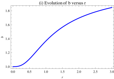
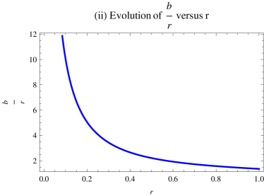
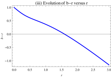
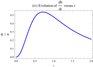
Figure 1: Plots of shape function in teleparallel case: (i) $b$ versus $r$, (ii) $\frac{b}{r}$ versus $r$, (iii) $b-r$ versus $r$, (iv) $\frac{db}{dr}$ versus $r$.

In order to examine the geometry of wormhole, we draw the shape function taking different conditions in Figure 1. We choose arbitrarily the values of model parameters, such as, $\phi=0.5,~{}M=15$ and $c=1$. Figure 1(i) represents the evolution of shape function in increasing manner versus $r$. For asymptomatically flat condition, we draw $\frac{b}{r}$ with respect to increasing $r$. It can be seen from plot (ii) that $\frac{b}{r}$ approaches towards $0$ as $r\rightarrow 0$. This implies that asymptotically flat condition for wormhole construction is satisfied. In plot (iii), we draw $b-r$ versus $r$ to find out throat radius. It is noted that throat radius is that minimum value for which $b-r$ cuts the $r$-axis. In this case, the throat radius is obtained as $r_{0}=1.6$. This plot satisfies the condition $1-\frac{b}{r}>0$ for $r>r_{0}$. In Figure 1(iv), we plot the first derivative of $b(r)$ with respect to $r$ to check the validity of condition $b^{\prime}(r_{0})<1$ which shows that the corresponding condition is satisfied. Thus, the shape function satisfies the required structure of the wormhole.

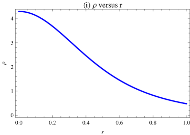
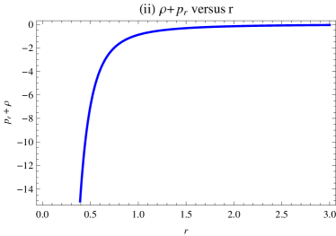
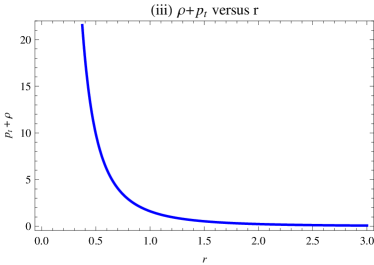
Figure 2: Plots of WEC in teleparallel case: (i) $\rho$ versus $r$, (ii) $\rho+p_{r}$ versus $r$, (iii) $\rho+p_{t}$ versus $r$.

Equations (18)-(20) are given as follows

$$\rho = \frac{M\sqrt{\phi}}{\pi^{2}(r^{2}+\phi)^{2}},$$ (27)

$$p_{r} = -\frac{1}{r^{3}}\left[\frac{M}{2\pi^{2}}\left(\frac{r\sqrt{\phi}}{r^{2}+\phi}+\tan^{-1}(\frac{r}{\sqrt{\phi}})\right)+c\right],$$ (28)

$$p_{t} = -\frac{1}{2r^{2}}\left[\frac{M\sqrt{\phi}}{\pi^{2}(r^{2}+\phi)^{2}}-\frac{1}{r}\left\{\frac{M}{2\pi^{2}}\left(\frac{r\sqrt{\phi}}{r^{2}+\phi}+\tan^{-1}(\frac{r}{\sqrt{\phi}})\right)+c\right\}\right].$$ (29)

The behavior of WEC ($\rho,~{}\rho+p_{r}$ and $\rho+p_{t}$) versus $r$ is shown in Figure 2. The curves of $\rho,~{}\rho+p_{t}$ represent positively decreasing behavior for increasing $r$ while $\rho+p_{r}$ indicates negative behavior which shows the violation of WEC. Thus no physically acceptable wormhole solution is obtained in teleparallel case. These results are compatible with the results of [14].

Case II: $\alpha\neq 0$

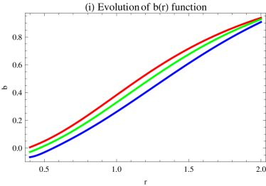
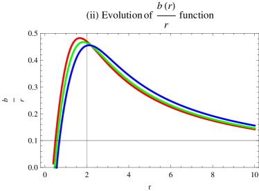
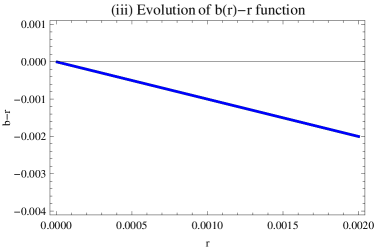
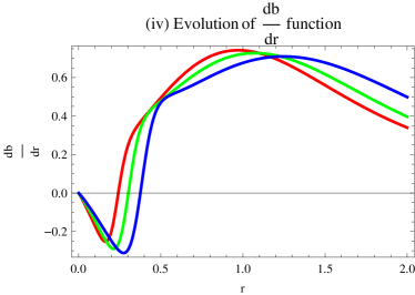
Figure 3: Plots of shape function in $f(T)$ case: red curve for $\alpha=-2$, green curve for $\alpha=-3$, blue curve for $\alpha=-5$ (i) $b$ versus $r$, (ii) $\frac{b}{r}$ versus $r$, (iii) $b-r$ versus $r$, (iv) $\frac{db}{dr}$ versus $r$.

The case $\alpha\neq 0$ leads to the extended teleparallel gravity. Inserting Eq.(24) in (23), we obtain the following differential equation

$$\frac{r^{2}M\sqrt{\phi}}{\pi^{2}(r^{2}+\phi)^{2}} = b^{\prime}\left\{1+\frac{4\alpha}{r^{2}}\left(2-\frac{b}{r}-2\sqrt{1-\frac{b}{r}}\right)\right\}-\frac{4\alpha}{r^{2}}\left(1-\frac{b}{r}-\sqrt{1-\frac{b}{r}}\right)$$ (30)

$$\times \left[4\left(1-\sqrt{1-\frac{b}{r}}\right)-\frac{2b}{r}+\frac{b^{\prime}r-b}{r}\left(1-\frac{1}{\sqrt{1-\frac{b}{r}}}\right)\right].$$

We check the behavior of shape function and flaring out conditions numerically through graphs by taking same values of parameters along with three different values of $\alpha$ such as $\alpha=-2,~{}-3,~{}-5$ and initial value as $f(2.2)=1$. Figure 3(i) represents increasing behavior of the shape function versus $r$. In the right graph (ii), $\frac{b}{r}$ versus $r$ shows that $\frac{b}{r}$ approaches to zero as we increase $r$ which represents that asymptomatically flatness is obtained. To locate throat of the wormhole, we plot $b(r)-r$ versus $r$ as shown in the (iii) plot of Figure 3. In this plot, the throat is located at very small values of $r$. The first derivative of shape function is also plotted versus $r$ as shown in (iv) plot which indicates that $\frac{db}{dr}$ at $r_{0}$ satisfies the condition, $b^{\prime}(r_{0})<1$. Thus similar to teleparallel case, shape function satisfies the conditions of wormhole geometry.

To check the behavior of WEC for power-law model, the expressions of matter content using Eqs.(18)-(20) are given by

$$\rho = \frac{b^{\prime}}{r^{2}}\left\{1+\frac{4\alpha}{r^{2}}\left(2-\frac{b}{r}-2\sqrt{1-\frac{b}{r}}\right)\right\}-\frac{4\alpha}{r^{2}}\left(1-\frac{b}{r}-\sqrt{1-\frac{b}{r}}\right)$$ (31)

$$\times \left[4\left(1-\sqrt{1-\frac{b}{r}}\right)-\frac{2b}{r}+\frac{b^{\prime}r-b}{r}\left(1-\frac{1}{\sqrt{1-\frac{b}{r}}}\right)\right],$$

$$p_{r} = -\frac{b}{r^{3}}\left\{1+\frac{4\alpha}{r^{2}}\left(2-\frac{b}{r}-2\sqrt{1-\frac{b}{r}}\right)\right\},$$ (32)

$$p_{t} = -\frac{1}{2r^{2}}\left(b^{\prime}-\frac{b}{r}\right)\left\{1+\frac{4\alpha}{r^{2}}\left(2-\frac{b}{r}-2\sqrt{1-\frac{b}{r}}\right)\right\}-\frac{2\alpha}{r^{4}}\left(1-\frac{b}{r}\right.$$ (33)

$$- \left.\sqrt{1-\frac{b}{r}}\right)\left[4\left(1-\sqrt{1-\frac{b}{r}}\right)-\frac{2b}{r}+\frac{b^{\prime}r-b}{r}\left(1-\frac{1}{\sqrt{1-\frac{b}{r}}}\right)\right].$$

Figure 4 represents graph of WEC expressions versus $r$ which show that $\rho$ and $\rho+p_{t}$ show decreasing behavior but remain positive. For $\alpha=-2,~{}\rho$ indicates negative value at $r\leq 0.52$. The behavior of $\rho+p_{r}$ is negative but there exist some part of the curves in positive panel of plot. Thus there exist possibility to have micro or tiny wormhole.

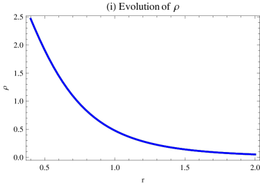
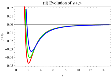
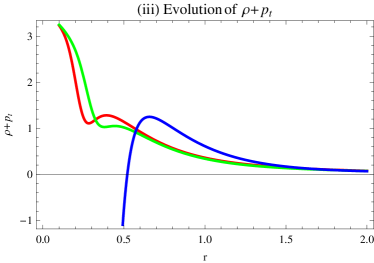
Figure 4: Plots of WEC in $f(T)$ case: red curve for $\alpha=-2$, green curve for $\alpha=-3$, blue curve for $\alpha=-5$ (i) $\rho$ versus $r$, (ii) $\rho+p_{r}$ versus $r$, (iii) $\rho+p_{t}$ versus $r$.

5.2 For Power-law $b(r)$ Model

Here, we examine the wormhole solution by considering a specific shape function in terms of power-law form and construct $f(T)$ function in the NCL background. We take the following particular shape function [10, 25]

$$b(r)=r_{0}\left(\frac{r}{r_{0}}\right)^{\gamma},$$ (34)

where $\gamma$ is any constant. To meet the wormhole geometry, it can be seen that $b^{\prime}(r_{0})<1$ implies that $b^{\prime}(r_{0})=\gamma<1$ and $b(r_{0})=r_{0}$ holds. The asymptotically flat spacetime is also obtained for this shape function, i.e., $\frac{b(r)}{r}=r_{0}^{1-\gamma}r^{\gamma-1}\rightarrow 0$ as $r\rightarrow\infty$. Substituting the values of $\rho_{{}_{NCL}}$ and $b(r)$ from Eqs.(22) and (34) in (18), we obtain the following differential equation

$$\frac{1}{r}\left[1-\left(\frac{r}{r_{0}}\right)^{\gamma-1}-\sqrt{1-\left(\frac{r}{r_{0}}\right)^{\gamma-1}}\right]\frac{f^{\prime\prime}}{T^{\prime}}+\frac{\gamma}{r^{2}}\left(\frac{r}{r_{0}}\right)^{\gamma-1}\frac{f^{\prime}}{T^{\prime}}-\frac{1}{r}$$

$$\times\left[1-\left(\frac{r}{r_{0}}\right)^{\gamma-1}-\sqrt{1-\left(\frac{r}{r_{0}}\right)^{\gamma-1}}\right]\frac{T^{\prime\prime}f^{\prime}}{T^{\prime 2}}=\frac{M\sqrt{\phi}}{\pi^{2}(r^{2}+\phi)^{2}},$$ (35)

where

$$T = \frac{2}{r^{2}}\left[2-\left(\frac{r}{r_{0}}\right)^{\gamma-1}-2\sqrt{1-\left(\frac{r}{r_{0}}\right)^{\gamma-1}}\right],$$

$$T^{\prime} = -\frac{2}{r^{3}}\left[4\left(1-\sqrt{1-\left(\frac{r}{r_{0}}\right)^{\gamma-1}}\right)-2\left(\frac{r}{r_{0}}\right)^{\gamma-1}+(\gamma-1)\right.$$

$$\times \left.\left(\frac{r}{r_{0}}\right)^{\gamma-1}\left(1-\frac{1}{\sqrt{1-\left(\frac{r}{r_{0}}\right)^{\gamma-1}}}\right)\right],$$

$$T^{\prime\prime} = \frac{12}{r^{4}}\left[2\left(1-\sqrt{1-\left(\frac{r}{r_{0}}\right)^{\gamma-1}}\right)-\left(\frac{r}{r_{0}}\right)^{\gamma-1}-\frac{(\gamma-1)(\gamma-6)}{6}\right.$$

$$\times \left.\left(\frac{r}{r_{0}}\right)^{\gamma-1}\left(1-\frac{1}{\sqrt{1-\left(\frac{r}{r_{0}}\right)^{\gamma-1}}}\right)+\frac{(\gamma-1)^{2}}{12}\left(\frac{r}{r_{0}}\right)^{2(\gamma-1)}\right.$$

$$\times \left.\left(1-\left(\frac{r}{r_{0}}\right)^{\gamma-1}\right)^{-\frac{3}{2}}\right].$$

We evaluate $f(T)$ function numerically and draw its plot as well as WEC versus $T$ and $r$ respectively, as shown in Figure 5. Keeping the same values of NCL parameters along with $\gamma=0.5$ for three values of throat radius $r_{0}=0.93,~{}0.95,~{}0.99$. The plot (i) indicates the positively decreasing behavior of $f$.

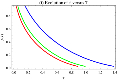
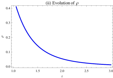
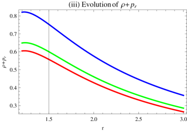
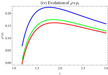
Figure 5: Plots of $f(T)$ and WEC: red curve for $r_{0}=0.93$, green curve for $r_{0}=0.95$, blue curve for $r_{0}=0.99$ (i) $f(T)$ versus $T$, (ii) $\rho$ versus $r$, (iii) $\rho+p_{r}$ versus $r$, (iv) $\rho+p_{t}$ versus $r$.

The expressions for WEC become

$$\rho = \frac{\gamma}{r^{2}}\left(\frac{r}{r_{0}}\right)^{\gamma-1}\frac{f^{\prime}}{T^{\prime}}+\frac{1}{r}\left(1-\left(\frac{r}{r_{0}}\right)^{\gamma-1}-\sqrt{1-\left(\frac{r}{r_{0}}\right)^{\gamma-1}}\right)$$ (36)

$$\times \left(\frac{f^{\prime\prime}}{T^{\prime}}-\frac{T^{\prime\prime}f^{\prime}}{T^{\prime 2}}\right),$$

$$\rho+p_{r} = \frac{\gamma-1}{r^{2}}\left(\frac{r}{r_{0}}\right)^{\gamma-1}\frac{f^{\prime}}{T^{\prime}}+\frac{1}{r}\left(1-\left(\frac{r}{r_{0}}\right)^{\gamma-1}-\sqrt{1-\left(\frac{r}{r_{0}}\right)^{\gamma-1}}\right)$$ (37)

$$\times \left(\frac{f^{\prime\prime}}{T^{\prime}}-\frac{T^{\prime\prime}f^{\prime}}{T^{\prime 2}}\right),$$

$$\rho+p_{t} = \frac{\gamma+1}{2r^{2}}\left(\frac{r}{r_{0}}\right)^{\gamma-1}\frac{f^{\prime}}{T^{\prime}}+\frac{1}{2r}\left(1-\left(\frac{r}{r_{0}}\right)^{\gamma-1}-\sqrt{1-\left(\frac{r}{r_{0}}\right)^{\gamma-1}}\right)$$ (38)

$$\times \left(\frac{f^{\prime\prime}}{T^{\prime}}-\frac{T^{\prime\prime}f^{\prime}}{T^{\prime 2}}\right).$$

Figure 5(ii)-(iv) shows the plots of these expressions versus $r$. This represents that $\rho,~{}\rho+p_{r},~{}\rho+p_{t}$ indicate positive behavior of these expressions. Thus, physically acceptable wormhole solutions are obtained for the specific shape function where the basic role is played by effective energy-momentum tensor.

6 Equilibrium Conditions

To discuss the equilibrium configuration of the wormhole solutions, we consider the generalized Tolman-Oppenheimer-Volkov equation [26, 27]

$$\frac{dp_{r}}{dr}+\frac{\sigma^{\prime}}{2}(\rho+p_{r})+\frac{2}{r}(p_{r}-p_{t})=0,$$ (39)

for the metric $ds^{2}=\textmd{diag}(e^{\sigma(r)},-e^{\mu(r)},-r^{2},-r^{2}\sin^{2}\theta)$. Ponce de Le$\acute{o}$n suggested this equation for anisotropic mass distribution as follows

$$\frac{2}{r}(p_{t}-p_{r})-\frac{e^{\frac{\mu-\sigma}{2}}\mathcal{M}_{{}_{eff}}}{r^{2}}(\rho+p_{r})-\frac{dp_{r}}{dr}=0.$$ (40)

Here $\mathcal{M}_{{}_{eff}}=\frac{1}{2}r^{2}e^{\frac{\sigma-\mu}{2}}\sigma^{\prime}$ is the effective gravitational mass which is measured from throat to some arbitrary radius $r$. This equation indicates the equilibrium configuration for the wormhole solutions by taking gravitational, hydrostatic as well as anisotropic force due to anisotropic matter distribution. Using Eq.(40), these forces are defined respectively as

$$\mathcal{F}_{gf}=-\frac{\sigma^{\prime}(\rho+p_{r})}{2},\quad\mathcal{F}_{hf}=-\frac{dp_{r}}{dr},\quad\mathcal{F}_{af}=\frac{2(p_{t}-p_{r})}{r}.$$

For the wormhole solutions to be in equilibrium, it is required that

$$\mathcal{F}_{gf}+\mathcal{F}_{hf}+\mathcal{F}_{af}=0.$$ (41)

It is noted here that $\sigma$ represents the gravitational redshift which is taken as constant, i.e., $\sigma=2\Psi$ leads to $\sigma^{\prime}=0$ for constant $\Psi$. This yields $\mathcal{F}_{gf}$ becomes zero and we are left with hydrostatic and anisotropic forces with corresponding equilibrium condition $\mathcal{F}_{hf}+\mathcal{F}_{af}=0$. For teleparallel, specific $f(T)$ and $b(r)$ cases, $\mathcal{F}_{hf}$ and $\mathcal{F}_{af}$ takes the following form respectively

$$\mathcal{F}_{hf} = -\frac{3}{r^{4}}\left[\frac{M}{2\pi^{2}}\left(\frac{r\sqrt{\phi}}{r^{2}+\phi}+\tan^{-1}\left(\frac{r}{\sqrt{\phi}}\right)\right)+c\right]+\frac{1}{r^{3}}\left[\frac{M\sqrt{\phi}(5r^{3}+3\phi)}{2\pi^{2}r^{3}(r^{2}+\phi)^{2}}\right.$$

$$- \left.\frac{3c}{r^{4}}-\frac{3M}{2\pi r^{4}}\tan^{-1}\left(\frac{r}{\sqrt{\phi}}\right)\right],$$

$$\mathcal{F}_{af} = -\frac{1}{r^{3}}\left[\frac{M\sqrt{\phi}}{\pi^{2}(r^{2}+\phi)^{2}}-\frac{3}{r}\left\{\frac{M}{2\pi^{2}}\left(\frac{r\sqrt{\phi}}{r^{2}+\phi}+\tan^{-1}\left(\frac{r}{\sqrt{\phi}}\right)\right)+c\right\}\right],$$

$$\mathcal{F}_{hf} = \left(\frac{b^{\prime}}{r^{3}}-\frac{3b}{r^{4}}\right)\left\{1+\frac{4\alpha}{r^{2}}\left(2-\frac{b}{r}-2\sqrt{1-\frac{b}{r}}\right)\right\}+\frac{b}{r^{6}}\left[-8\alpha\right.$$

$$\times \left.\left(2-\frac{b}{r}-2\sqrt{1-\frac{b}{r}}\right)-\frac{4\alpha(b^{\prime}r-b)}{r}\left(1-\frac{1}{\sqrt{1-\frac{b}{r}}}\right)\right],$$

$$\mathcal{F}_{af} = -\frac{1}{r^{3}}\left[\left(b^{\prime}-\frac{3b}{r}\right)\left\{1+\frac{4\alpha}{r^{2}}\left(2-\frac{b}{r}-2\sqrt{1-\frac{b}{r}}\right)\right\}+\frac{4\alpha}{r}\left(\frac{b}{r}-1\right.\right.$$

$$+ \left.\left.\sqrt{1-\frac{b}{r}}\right)\left[4\left(1-\sqrt{1-\frac{b}{r}}\right)-\frac{2b}{r}+\frac{b^{\prime}r-b}{r}\left(1-\frac{1}{\sqrt{1-\frac{b}{r}}}\right)\right]\right],$$

$$\mathcal{F}_{hf} = \frac{\gamma-3}{r^{3}}\left(\frac{r}{r_{0}}\right)^{\gamma-1}\frac{f^{\prime}}{T^{\prime}}+\frac{1}{r^{2}}\left(\frac{r}{r_{0}}\right)^{\gamma-1}\left(\frac{f^{\prime\prime}}{T^{\prime}}-\frac{T^{\prime\prime}f^{\prime}}{T^{\prime 2}}\right),$$

$$\mathcal{F}_{af} = \frac{3-\gamma}{r^{3}}\left(\frac{r}{r_{0}}\right)^{\gamma-1}\frac{f^{\prime}}{T^{\prime}}+\frac{1}{r^{2}}\left(\left(\frac{r}{r_{0}}\right)^{\gamma-1}-1+\sqrt{1-\left(\frac{r}{r_{0}}\right)^{\gamma-1}}\right)$$

$$\times \left(\frac{f^{\prime\prime}}{T^{\prime}}-\frac{T^{\prime\prime}f^{\prime}}{T^{\prime 2}}\right).$$

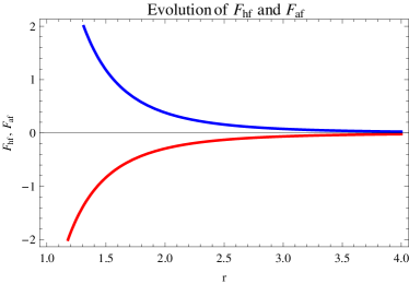
Figure 6: Plot of $\mathcal{F}_{hf}$ and $\mathcal{F}_{af}$ in teleparallel case versus $r$: red curve represents $\mathcal{F}_{hf}$ and blue curve represents $\mathcal{F}_{af}$.

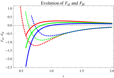
Figure 7: Plot of $\mathcal{F}_{hf}$ (dotted) and $\mathcal{F}_{af}$ (solid) in specific $f(T)$ case versus $r$.

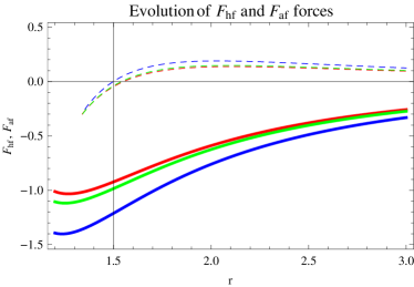
Figure 8: Plot of $\mathcal{F}_{hf}$ (dotted) and $\mathcal{F}_{af}$ (solid) in specific $b(r)$ case versus $r$.

We plot these equations for the obtained wormhole solutions as shown in Figures 6-8 respectively. For teleparallel case, we examine that both hydrostatic and anisotropic forces show same behavior but in opposite direction and thus balance each other. This implies that the wormhole solution in teleparallel case satisfy equilibrium condition. In case of power-law $f(T)$ function, this condition shows wormhole solutions in equilibrium state as $r$ increases. For smaller values of $r$, these solutions do not satisfy equilibrium condition properly or we may remark that these solutions are less stable. For specific $b(r)$ function, forces $\mathcal{F}_{hf}$ and $\mathcal{F}_{af}$ do not balance each other. Since all the curves are in opposite manner having no similarity. Therefore the physically acceptable wormhole solutions are not in equilibrium form.

7 Conclusion

A wormhole represents shortcut distance to connect different regions of the universe. To study these solutions, the violation of NEC plays the key role which is associated with the exotic matter. To minimize the usage of exotic matter is an important issue which leads to explore a realistic model in favor of wormhole. In this paper, we have studied static spherically symmetric wormhole solutions in $f(T)$ gravity by taking NCL background. We have developed the $f(T)$ field equations in terms of effective energy-momentum tensor by taking non-diagonal tetrad and proved that this tensor is responsible for the WEC violation. By imposing the condition on matter content to thread the wormhole solutions, we have assumed either the $f(T)$ or shape function and constructed the other one. The graphical behavior of these solutions is discussed.

For power-law $f(T)$ model, we have discussed two cases: teleparallel gravity ad $f(T)$ gravity in quadratic form. Both models satisfied the conditions for wormhole geometry on shape function. The WEC condition is violated for first case while possibility of tiny wormhole solution is examined for $f(T)$ case. In another case of particular form of power-law shape function, we have analyzed the wormhole geometry. We have found physically acceptable wormhole solutions as WEC satisfied in this case. Also, we have examined the stability of these wormhole solutions with the help of generalized Tolman-Oppenheimer-Volkov equation. We have found that teleparallel NCL wormhole solutions are stable while $f(T)$ NCL wormhole solutions are less stable. For the wormhole solutions in specific shape function case, we have obtained unstable solutions.

Bhar and Rahaman [GR] investigated whether the wormhole solutions exists in different dimensional non-commutative inspired spacetimes with Lorentzian distribution. For four and five dimensional spacetime, there exist wormhole solutions while no solution for higher dimensions. They observed a stable wormhole, i.e., satisfying flare out conditions and violating energy conditions for four dimensions. It is interesting to note that for underlying case, we also obtain asymptotically flat and stable solutions in telaparallel case, i.e., the behavior of all conditions is identical. The wormhole solutions [11] in the background of NC geometry give physically acceptable wormhole solutions in $f(T)$ gravity case while in teleparallel case, energy conditions violate as per requirement. However this work is done taking diagonal tetrad which is less in interest for spherical symmetry. In case of Lorentzian distributed NC background, we have found physically acceptable wormhole solutions in more stable form. We have used non-diagonal tetrad which is the favorable choice for spherically symmetry. The NC wormholes in $f(R)$ gravity with Lorentzian distributed are discussed by Rahaman et al. [28]. They studied the same cases and found violation of energy conditions in all cases. That is no physically acceptable solutions in $f(R)$ gravity. However, we have found physically acceptable as well as stable solutions.

References

- [1] Kamenshchik, A.Y., Moschella, U. and Pasquier, V.: Phys. Lett. B 511(2001)265; Li, M.: Phys. Lett. B 603(2004)1; Cai, R.G.: Phys. Lett. B 657(2007)228.
- [2] Wei, H.: Commun. Theor. Phys. 52(2009)743; Sheykhi, A. and Jamil, M.: Gen. Relativ. Gravit. 43(2011)2661.
- [3] Ferraro, R. and Fiorini, F.: Phys. Rev. D 75(2007)084031; ibid. 78(2008)124019.
- [4] Wang, T.: Phys. Rev. D 84(2011)024042; JCAP11(2011)033; Daouda, M.H., Rodrigues, M.E. and Houndjo, M.J.S.: Eur. Phys. J. C. 71(2011)1817; Ferraro, R. and Fiorini, F.: Phys. Rev. D 84(2011)083518; Daouda, M.H., Rodrigues, M.E. and Houndjo, M.J.S.: Eur. Phys. J. C 72(2012)1890; Gonz lez, P.A., Saridakis, E.N. and V squez, Y.: JHEP 53(2012)2012; Nashed, G.G.L.: Chinese Phys. Lett. 29(2012)050402; Iorio, L. and Saridakis, E.N.: Mon. Not. Roy. Astron. Soc. 427(2012)1555; Capozziello, S. et al.: JHEP 1302(2013)039;Atazadeh, K. and Mousavi, M.: Eur. Phys. J. C 73(2013)2272; Nashed, G.G.L.: Phys. Rev. D 88(2013)104034; Paliathanasis, A.: Phys. Rev. D 89(2014)104042; Aftergood, J. and DeBenedictis, A.: Phys. Rev. D 90(2014)124006; Gonz lez, P.A., Saavedra, J. and V squez, Y.: arXiv:1411.2193, arXiv:1501.00365; Nashed, G.G.L.: Gen Relativ Gravit 45(2013)1887.
- [5] Kim, S-W. and Lee, H.: Phys. Rev. D 63(2001)064014; Rahaman, F., Islam, S., Kuhfittig, P.K.F. and Ray, S.: Phys. Rev. D 86(2012)106010; Sharif, M. ad Jawad, A.: Eur. Phys. J. Plus 129(2014)15; Rahaman, F., et al.: Int. J. Theor. Phys. 53(2014)1910.
- [6] Böhmer, C.G., Harko, T. nad Lobo, F.S.N.: Phys. Rev. D 85(2012)044033.
- [7] Jamil, M., Momeni, D. and Myrzakulov, R.: Eur. Phys. J. C 73(2013)2267.
- [8] Sharif, M. and Rani, S.: Gen. Relativ. Gravit. 45(2013)2389.
- [9] Rahaman, F., Islam, S., Kuhfittig, P.K.F. and Ray, S.: Phys. Rev. D 86(2012)106010.
- [10] Jamil, M. et al.: J. Kor. Phys. Soc. 65(2014)97.
- [11] Sharif, M. and Rani, S.: Phys. Rev. D 88(2013)123501.
- [12] Sharif, M. and Rani, S.: Eur. Phys. J. Plus 129(2014)237.
- [13] Sharif, M. and Rani, S.: Adv. High Energy Phys. 2014(2014)691497.
- [14] Bhar, P. and Rahaman, F.: Eur. Phys. J. C 74(2014)3213.
- [15] Misner, C.W. and Wheeler, J.A.: Ann. Phys. 2(1957)525.
- [16] Wheeler, J.A.: Geometrodynamics (Acedamic Press, 1962).
- [17] Morris, M. and Thorne, K.: Am. J. Phys. 56(1988)395.
- [18] Visser, M., Kar, S. and Dadhich, N.: Phys. Rev. Lett. 90(2003)201102.
- [19] De Andrade, V. C. and Pereira, J.G.: Gen. Relat. Gravit. 30(1998)263; Aldrovandi, R. and Pereira, J.G.: Teleparallel Gravity: An Introduction (Springer, 2012).
- [20] Li, B., Sotiriou, T.P. and Barrow, J.D.: Phys. Rev. D 83(2011)064035; ibid. 83(2011)104017; Sotiriou, T.P., Li, B. and Barrow, J.D.: Phys. Rev. D 83(2011)104030; Liu, D. and Rebouças, M.J.: Phys. Rev. D 86(2012)083515.
- [21] Böhmer, C.G., Mussa, A. and Tamanini, N.: Class. Quantum Grav. 28(2011)245020.
- [22] Nicolini, P., Smailagic, A. and Spalluci, E.: Phys. Lett. B 632(2006)547.
- [23] Rahaman, F., Kuhfittig, P.K.F., Ray, S. and Islamd, N.: Eur. Phys. J. C 74(2014)2750.
- [24] Kuhfittig, P.K.F.: Eur. Phys. J. C 74(2014)2818.
- [25] Jamil, M. and Farooq, M.U.: Int. J. Theor. Phys. 49(2010)835; Farooq, M., Akbar, M. and Jamil, M.: AIP Conf. Proc. 1295(2010)176.
- [26] Rahaman, F., Kuhfittig, P.K.F., Ray, S. and Islamd, N.: Eur. Phys. J. C 74(2014)2750.
- [27] Kuhfittig, P.K.F.: Eur. Phys. J. C 74(2014)2818.
- [28] Rahaman, F., Banerjee, A., Jamil, M., Yadav, A.K. and Idris, H.: Int. J. Theor. Phys. 53(2014)1910.