Scheduling Wireless Links by Graph Multicoloring in the Physical Interference Model

Abstract

Scheduling wireless links for simultaneous activation in such a way that all transmissions are successfully decoded at the receivers and moreover network capacity is maximized is a computationally hard problem. Usually it is tackled by heuristics whose output is a sequence of time slots in which every link appears in exactly one time slot. Such approaches can be interpreted as the coloring of a graph’s vertices so that every vertex gets exactly one color. Here we introduce a new approach that can be viewed as assigning multiple colors to each vertex, so that, in the resulting schedule, every link may appear more than once (though the same number of times for all links). We report on extensive computational experiments, under the physical interference model, revealing substantial gains for a variety of randomly generated networks.

Keywords: Wireless mesh networks, Link scheduling, Physical interference model, Graph coloring, Graph multicoloring.

1 Introduction

Let $L$ be a set of wireless links, each link $i\in L$ characterized by a sender node $s_{i}$ and a receiver node $r_{i}$. Depending on the spatial disposition of such nodes, activating more than one link simultaneously creates interference that may hamper the receivers’ ability to decode what they receive. In the physical interference model [1], the chief quantity governing receiver $r_{i}$’s ability to decode what it receives from $s_{i}$ when all links of a set $S$ containing link $i$ are active is the signal-to-interference-and-noise ratio (SINR), given by

$$\mathrm{SINR}(r_{i},S)=\frac{P/d^{\alpha}_{s_{i}r_{i}}}{N+\sum_{j\in S\setminus\{i\}}P/d^{\alpha}_{s_{j}r_{i}}},$$ (1)

where $P$ is a sender’s transmission power (assumed the same for all senders), $N$ is the noise floor, $d_{ab}$ is the Euclidean distance between nodes $a$ and $b$, and $\alpha>2$ determines the law of power decay with Euclidean distance. We say that a nonempty subset $S$ of $L$ is feasible if no two of its members share a node (in case $|S|>1$) and moreover $\mathrm{SINR}(r_{i},S)\geq\beta$ for all $i\in S$, where $\beta$ is a parameter related to a receiver’s decoding capabilities (assumed the same for all receivers) and is chosen so that $\beta>1$.

Several strategies have been devised to maximize network capacity, either through the self-contained scheduling of the links in $L$ for activation [2, 3, 4, 5, 6, 7, 8, 9, 10, 11, 12, 13, 14, 15] or by combining link scheduling with other techniques [16, 17, 18, 19, 20, 21, 22]. All these strategies revolve around formulations as NP-hard optimization problems, so all rely on some form of heuristic procedure drawing inspiration from various sources, some merely intuitive, others more formally grounded on graph-theoretic notions. Often the problem is formulated in a spatial time-division multiple access (STDMA) framework, that is, assuming essentially that time is divided into time slots, each one accommodating a certain number of simultaneous link activations. In this case, the problem is to find $T$ feasible subsets of $L$, here denoted by $S_{1},S_{2},\ldots,S_{T}$, minimizing $T$ while ensuring that every link appears in exactly one of the $T$ subsets.

There is a sense in which this formulation can be interpreted in the context of coloring a graph’s vertices. Specifically, if we regard the links to be scheduled as vertices in a graph, and furthermore say that no two vertices of a group are neighbors of each other if the corresponding set of links is feasible, then the schedule given by the sequence $S_{1},S_{2},\ldots,S_{T}$ of feasible link sets establishes a coloring of the graph’s vertices with $T$ colors in which all vertices in $S_{k}$ get color $k$. This interpretation suggests a generalization of the above formulation that requires every link to appear not in exactly one of the $T$ subsets but in any number $q$ of subsets, provided this number is the same for all links. In this generalized formulation, the goal is no longer to minimize $T$, but rather to find the values of $T$ and $q$ that minimize the ratio $T/q$. Returning to the vertex-coloring interpretation, now a vertex receives $q$ (out of $T$) distinct colors, each relative to the time slot in which the corresponding link is scheduled to be activated (i.e., $q$ of the subsets $S_{1},S_{2},\ldots,S_{T}$).

The potential advantages of this multicoloring-based formulation are tantalizing. If the original formulation leads to a number $T$ of slots while the new one leads to $T^{\prime}>T$ slots for some $q>1$, the latter schedule is preferable to the former, even though it requires more time slots, provided only that $T^{\prime}/q<T$ (or $qT>T^{\prime}$). To see that this is so, first note that the longer schedule promotes an overall number of link activations given by $q|L|$ in $T^{\prime}$ time slots. In order for the shorter schedule to achieve this same number of activations, it would have to be repeated $q$ times in a row, taking up $qT>T^{\prime}$ time slots.

The possibility of multicoloring-based link scheduling in the physical interference model seems to have been overlooked so far, despite the recent demonstration of its success in the protocol-based interference model [22]. Here we introduce a heuristic framework to obtain multicoloring-based schedules from the single-color schedules produced by any rank-based heuristic (i.e., one that decides the time slot in which to activate a given link based on how it ranks relative to the others with respect to some criterion). We use two iconic single-color heuristics (GreedyPhysical [3], for its simplicity, and ApproxLogN [8, 15], for its role in establishing new bounds on network capacity), as well as a third one that we introduce in response to improvement opportunities that we perceived in the former two. Incidentally, the latter heuristic, called MaxCRank, is found to perform best both as a stand-alone, single-color strategy and as a base for the multicoloring scheme.

2 Single-color schedules

Rank-based heuristics for single-color scheduling are usually monotonic, in the sense that first $S_{1}$ is determined, then $S_{2}$ out of the set $R$ of links that remain to be scheduled, then $S_{3}$ out of a smaller $R$, and so on, until $R$ becomes empty. Choosing a link to add to the current $S_{k}$ depends on the feasibility of the resulting set and also on a ranking criterion that is specific to each heuristic. The ranking criterion establishes the order in which the links in $R$ are to be considered for inclusion in $S_{k}$.

The following is the general outline of such a heuristic.

1. Let $k:=1$, $S_{k}:=\emptyset$, and $R:=L$. Order $R$ according to the ranking criterion.

2. If a link $i\in R$ exists such that $S_{k}\cup\{i\}$ is feasible, then move the top-ranking such $i$ from $R$ to $S_{k}$ and go to Step 3. If none exists, then let $k:=k+1$, $S_{k}:=\emptyset$, and go to Step 2.

3. If $R\neq\emptyset$, then reorder $R$ according to the ranking criterion and go to Step 2.

4. Let $T:=k$ and output $S_{1},S_{2},\ldots,S_{T}$.

Steps 1–4 amount to scanning the set $R$ of unscheduled links and moving to the current $S_{k}$ (in Step 2) the top-ranking link $i\in R$ whose inclusion in $S_{k}$ preserves feasibility. Whenever such a move does occur, an opportunity is presented for $R$ to be reordered (in Step 3) according to the ranking criterion.

It is easy to see that both GreedyPhysical and ApproxLogN can be cast in this sequence of steps in a straightforward manner. The ranking criterion for GreedyPhysical is nonincreasing and refers, for link $i$, to the number of links in $L$ with which $i$ can never share a time slot; that is, links $j\in L$ such that $\{i,j\}$ is infeasible. It is then an immutable ranking criterion and consequently the reordering in Step 3 is moot. As for ApproxLogN, its ranking criterion is nondecreasing, but now refers to the Euclidean distance between the sender and the receiver in each link. This criterion, too, is fixed and as such renders the reordering in Step 3 once again moot.

We now introduce a new heuristic that can also be viewed as instantiating Steps 1–4, but with a ranking criterion that is both more stringent than the two just described and also inherently dynamic, thus justifying the reordering in Step 3. We call it MaxCRank to highlight its core principle, which is to maximize the number of links in $R$ that still have a chance of joining the current $S_{k}$ (i.e., remain “Candidates”) once a decision is made on which one of them, say $i$, is to be moved from $R$ to $S_{k}$. The corresponding ranking criterion is nondecreasing and refers to the number of links $j\in R\setminus\{i\}$ for which $S_{k}\cup\{i,j\}$ is infeasible.

3 Multicoloring-based schedules

The link sets $S_{1},S_{2},\ldots,S_{T}$ output by Steps 1–4 of Section 2 promote a number of link activations given by $|L|$, one activation per link. If this schedule were to be repeated $q$ times in a row for some $q>1$, the total number of link activations would grow by a factor of $q$ and so would the number of time slots used. That the same growth law should apply both to how many links are activated and to how many time slots elapse indicates that the most basic scheduling unit is $S_{1},S_{2},\ldots,S_{T}$ itself, not any number of repetitions thereof.

However, activating the links in $S_{1}$ the second time around does not necessarily have to be restricted to time slot $T+1$. Instead, it may be possible to take advantage of some room left in previous time slots for at least one of the links in $S_{1}$. With this type of precaution in mind, advancing link activations in such a manner might result in a sequence of link sets $S_{1},S_{2},\ldots,S_{T^{\prime}}$ containing exactly $q$ activations of every link in $L$ for some $q>1$ but with $T<T^{\prime}<qT$. Clearly, in this case the most basic scheduling unit would be $S_{1},S_{2},\ldots,S_{T^{\prime}}$, not $S_{1},S_{2},\ldots,S_{T}$ any more. Not only this, but the new basic scheduling unit would be preferable to the previous one, since a total of $q|L|$ link activations would be attainable in fewer time slots ($T^{\prime}$ rather than $qT$).

A heuristic to find the greatest $q>1$ for which $T^{\prime}<qT$, if any exists, is simply to wrap Steps 1–4 in an outer loop that iterates along with $q=1,2,\ldots$ while preventing $S_{k}$ from being reset to $\emptyset$ any later than the first time it is considered. At the end of each iteration, say the $q$th, the value of $T^{\prime}$ is updated (to the number of time slots elapsed since the beginning) and the ratio $T^{\prime}/q$ is computed. The iterations continue while this ratio is strictly decreasing. At the end of the first iteration we get $T^{\prime}=T$, but successful further iterations will produce a sequence of strictly decreasing $T^{\prime}/q$ values. A new quantity of interest is then the gain $G$ incurred by the resulting heuristic, that is, the ratio of $T$ to the last $T^{\prime}/q$, hence $G=qT/T^{\prime}$. The least possible value of $G$, of course, is $G=1$, which corresponds to the case in which the iterations fail already for $q=2$.

4 Experimental setup

We give results for two families of randomly generated networks, henceforth referred to as type-I and type-II networks. As will become apparent, type-I networks are more realistic. We use type-II networks as well because they were used in the performance evaluation of ApproxLogN [8, 15] and thus provide a more direct basis for comparison. A network’s number of nodes is henceforth denoted by $n$.

A type-I network is generated by first placing all $n$ nodes inside a square of side $\ell$ uniformly at random. A node’s neighbors are then determined as a function of the value of $d_{s_{i}r_{i}}$ for which $\mathrm{SINR}(r_{i},\{i\})=\beta$. Denoting such a distance by $\rho$ yields $\rho=(P/\beta N)^{1/\alpha}$, so a node’s neighbor set is the set of nodes to which the Euclidean distance does not surpass $\rho$. Any two nodes that are neighbors of each other become a link in $L$, sender and receiver being decided uniformly at random (so that a node may, e.g., be the sender in a link and the receiver in another). For fixed $n$, increasing $\ell$ causes the number of links, $|L|$, to decrease precipitously, though in the heavy-tailed manner of an approximate power law (Fig. 1). It also causes the network’s number of connected components to increase from about $1$ to nearly $n$ (a component per node) through a sharp transition in between (Fig. 2).

Figure 1: Average number of links in type-I networks as a function of the square side $\ell$ for $n=100$. All data points are averages over $1\,000$ network instances. Additional relevant parameters are $P=300$ mW, $N\approx 8\times 10^{-14}$ W (for a bandwidth of $20$ MHz at room temperature), $\alpha=4$, and $\beta=25$ dB.

Figure 2: Average number of connected components in type-I networks as a function of the square side $\ell$ for $n=100$. All data points are averages over $1\,000$ network instances. Additional relevant parameters are $P=300$ mW, $N\approx 8\times 10^{-14}$ W (for a bandwidth of $20$ MHz at room temperature), $\alpha=4$, and $\beta=25$ dB.

In a type-II network, the number $n$ of nodes is necessarily even. Of these, $n/2$ are senders and $n/2$ are receivers. A type-II network is generated by first placing the receivers uniformly at random inside a square of side $\ell$ and then, for each receiver, placing the corresponding sender inside a circle of radius $\rho$ centered at it, also uniformly at random. A type-II network has $n/2$ links and connected components. Varying $\ell$ affects interference only.

5 Results

We give results for all three single-color heuristics mentioned in Section 2, namely GreedyPhysical, ApproxLogN, and MaxCRank, and also for their multicoloring-based versions, obtained as explained in Section 3. These results are given as $T/|L|$ in the former case (the normalized schedule length, since $|L|$ is a clear upper bound on $T$), and as the gain $G$ in the latter.

The data in Fig. 3 refer to type-I networks and as such are given as a function of the square side $\ell$. The number of nodes is fixed throughout (at $n=100$), so the networks get sparser (fewer links, more connected components) as $\ell$ is increased. In the single-color cases (panel (a) of the figure), all three heuristics start out with $T=|L|$ for the very dense networks (very small $\ell$), but smaller densities quickly reduce interference so that $T$ falls significantly below $|L|$. MaxCRank is the best performer throughout, followed by GreedyPhysical and ApproxLogN. As for the heuristics’ multicoloring-based versions (panel (b)), there is practically no gain for the densest networks, but again this is reversed as interference abates with increasing $\ell$. MaxCRank is still the top performer and ApproxLogN the bottom one (in fact, the only of the three heuristics for which $G=1$ is sometimes attained).

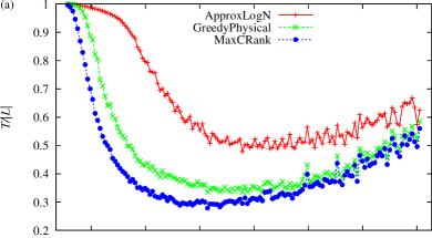
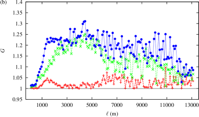
Figure 3: Performance of GreedyPhysical, ApproxLogN, and MaxCRank on type-I networks. Data are given for the heuristics’ single-color versions (a) and for their multicoloring-based versions (b). All data points are averages over $1\,000$ network instances. Confidence intervals are less than $1\%$ of the mean at the $95\%$ level, so error bars are omitted. All networks have $n=100$ nodes. Additional relevant parameters are $P=300$ mW, $N\approx 8\times 10^{-14}$ W (for a bandwidth of $20$ MHz at room temperature), $\alpha=4$, and $\beta=25$ dB.

The results for type-II networks, given in Fig. 4, are presented as a function of $|L|=n/2$, the number of links. Because $\ell$ is fixed throughout (at $\ell=1\,000$ m), increasing $|L|$ causes the impact of accumulated interference to be felt more severely. One consequence of this is that, for the single-color heuristics (panel (a) of the figure), $T$ increases almost linearly with $|L|$. Another consequence, now related to the multicoloring-based versions of the heuristics (panel (b)), is that gains above $1$ are increasingly hard to come by as $|L|$ is increased. MaxCRank continues to be the top performer in all cases, followed by GreedyPhysical, then by ApproxLogN.

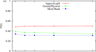
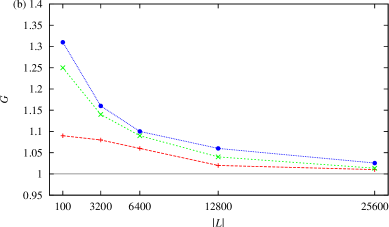
Figure 4: Performance of GreedyPhysical, ApproxLogN, and MaxCRank on type-II networks. Data are given for the heuristics’ single-color versions (a) and for their multicoloring-based versions (b). All data points are averages over $1\,000$ network instances. Confidence intervals are less than $1\%$ of the mean at the $95\%$ level, so error bars are omitted. All networks have $\ell=1\,000$ m. Additional relevant parameters are $P=300$ mW, $N\approx 8\times 10^{-14}$ W (for a bandwidth of $20$ MHz at room temperature), $\alpha=4$, and $\beta=25$ dB.

6 Discussion

Although it may at first seem striking that ApproxLogN has performed so poorly across most of our experiments, it should be kept in mind that this heuristic, in all likelihood, was never meant as a serious contender for single-color link scheduling. In fact, and as noted in Section 2, ApproxLogN approaches the checking of feasibility rather indirectly, verifying sufficient conditions for feasibility to hold instead of the property itself. This is bound to prevent ApproxLogN from scheduling links for activation when they could be scheduled. What must be kept in mind, then, is that the use of such indirect conditions has led to important performance and capacity bounds. ApproxLogN, therefore, remains an important contribution despite its performance in more practical settings.

What really is striking in our results, though, is the appearance of greater-than-$1$ gains practically across the board, particularly for MaxCRank or GreedyPhysical as the base, single-color heuristic. Link schedules, once determined, are meant to be used repetitively, so every link is already meant to be scheduled for activation over and over again, indefinitely. Conceptually, what our multicoloring-based wrapping of single-color heuristics tries to do is to intertwine some number of repetitions of a single-color schedule, taking up fewer time slots than the straightforward juxtaposition of the same number of repetitions of that schedule. By doing so, more link activations can be packed together in earlier time slots. As a consequence, the basic schedule to be used for indefinite repetition is now one that leads to higher network capacity and possibly higher throughput.

As we mentioned earlier, multicoloring-based link scheduling of the sort we have demonstrated has roots in the multicoloring of a graph’s vertices (as well as edges, in many cases). As such, a rich body of material, relating both to computational-complexity difficulties and to workarounds in important cases, is available. Further developments should draw on such knowledge, aiming to obtain more principled, and perhaps even better performing, heuristics.

Acknowledgments

The authors acknowledge partial support from CNPq, CAPES, and a FAPERJ BBP grant.

References

- [1] P. Gupta and P. R. Kumar. The capacity of wireless networks. IEEE T. Inform. Theory, 46:388–404, 2000.
- [2] K. Jain, J. Padhye, V. N. Padmanabhan, and L. Qiu. Impact of interference on multi-hop wireless network performance. In Proc. MobiCom, pages 66–80, 2003.
- [3] G. Brar, D. M. Blough, and P. Santi. Computationally efficient scheduling with the physical interference model for throughput improvement in wireless mesh networks. In Proc. MobiCom, pages 2–13, 2006.
- [4] W. Wang, Y. Wang, X.-Y. Li, W.-Z. Song, and O. Frieder. Efficient interference-aware TDMA link scheduling for static wireless networks. In Proc. MobiCom, pages 262–273, 2006.
- [5] T. Moscibroda, Y. A. Oswald, and R. Wattenhofer. How optimal are wireless scheduling protocols? In Proc. INFOCOM, pages 1433–1441, 2007.
- [6] D. Chafekar, V. S. A. Kumart, M. V. Marathe, S. Parthasarathy, and A. Srinivasan. Approximation algorithms for computing capacity of wireless networks with SINR constraints. In Proc. INFOCOM, pages 1166–1174, 2008.
- [7] Q.-S. Hua and F. C. M. Lau. Exact and approximate link scheduling algorithms under the physical interference model. In Proc. DIALM-FOMC, pages 45–54, 2008.
- [8] O. Goussevskaia, R. Wattenhofer, M. M. Halldorsson, and E. Welzl. Capacity of arbitrary wireless networks. In Proc. INFOCOM, pages 1872–1880, 2009.
- [9] P. Santi, R. Maheshwari, G. Resta, S. Das, and D. M. Blough. Wireless link scheduling under a graded SINR interference model. In Proc. FOWANC, pages 3–12, 2009.
- [10] C. Boyaci, B. Li, and Y. Xia. An investigation on the nature of wireless scheduling. In Proc. INFOCOM, pages 1–9, 2010.
- [11] D. Yang, X. Fang, G. Xue, A. Irani, and S. Misra. Simple and effective scheduling in wireless networks under the physical interference model. In Proc. GLOBECOM, pages 1–5, 2010.
- [12] C. H. P. Augusto, C. B. Carvalho, M. W. R. da Silva, and J. F. de Rezende. REUSE: a combined routing and link scheduling mechanism for wireless mesh networks. Comput. Commun., 34:2207–2216, 2011.
- [13] M. Leconte, J. Ni, and R. Srikant. Improved bounds on the throughput efficiency of greedy maximal scheduling in wireless networks. IEEE/ACM T. Network., 19:709–720, 2011.
- [14] Y. Shi, Y. T. Hou, S. Kompella, and H. D. Sherali. Maximizing capacity in multihop cognitive radio networks under the SINR model. IEEE T. Mobile Comput., 10:954–967, 2011.
- [15] O. Goussevskaia, M. M. Halldorsson, and R. Wattenhofer. Algorithms for wireless capacity. IEEE/ACM T. Network., 22:745–755, 2014.
- [16] R. L. Cruz and A. V. Santhanam. Optimal routing, link scheduling and power control in multihop wireless networks. In Proc. INFOCOM, pages 702–711, 2003.
- [17] M. Alicherry, R. Bhatia, and L. Li. Joint channel assignment and routing for throughput optimization in multi-radio wireless mesh networks. In Proc. MobiCom, pages 58–72, 2005.
- [18] J. Wang, P. Du, W. Jia, L. Huang, and H. Li. Joint bandwidth allocation, element assignment and scheduling for wireless mesh networks with MIMO links. Comput. Commun., 31:1372–1384, 2008.
- [19] A. Capone, G. Carello, I. Filippini, S. Gualandi, and F. Malucelli. Routing, scheduling and channel assignment in wireless mesh networks: optimization models and algorithms. Ad Hoc Netw., 8:545–563, 2010.
- [20] T. Kesselheim. A constant-factor approximation for wireless capacity maximization with power control in the SINR model. In Proc. SODA, pages 1549–1559, 2011.
- [21] I. Rubin, C.-C. Tan, and R. Cohen. Joint scheduling and power control for multicasting in cellular wireless networks. EURASIP J. Wirel. Comm., 2012:250, 2012.
- [22] F. R. J. Vieira, J. F. de Rezende, V. C. Barbosa, and S. Fdida. Scheduling links for heavy traffic on interfering routes in wireless mesh networks. Comput. Netw., 56:1584–1598, 2012.