Calibrating the $\alpha$ parameter of convective efficiency using observed stellar properties

Abstract

Context. Synthetic model atmosphere calculations are still the most commonly used tool when determining precise stellar parameters and stellar chemical compositions. Besides three-dimensional models that consistently solve for hydrodynamic processes, one-dimensional models that use an approximation for convective energy transport play the major role.

Aims. We use modern Balmer-line formation theory as well as spectral energy distribution (SED) measurements for the Sun and Procyon to calibrate the model parameter $\alpha$ that describes the efficiency of convection in our 1D models. Convection was calibrated over a significant range in parameter space, reaching from F-K along the main sequence and sampling the turnoff and giant branch over a wide range of metallicities. This calibration was compared to theoretical evaluations and allowed an accurate modeling of stellar atmospheres.

Methods. We used Balmer-line fitting and SED fits to determine the convective efficiency parameter $\alpha$. Both methods are sensitive to the structure and temperature stratification of the deeper photosphere.

Results. While SED fits do not allow a precise determination of the convective parameter for the Sun and Procyon, they both favor values significantly higher than 1.0. Balmer-line fitting, which we find to be more sensitive, suggests that the convective efficiency parameter $\alpha$ is $\approx 2.0$ for the main sequence and quickly decreases to $\approx 1.0$ for evolved stars. These results are highly consistent with predictions from 3D models. While the values on the main sequence fit predictions very well, measurements suggest that the decrease of convective efficiency as stars evolve to the giant branch is more dramatic than predicted by models.

1 Introduction

One-dimensional (1D) stellar model atmospheres are widely used for determining basic physical parameters, such as effective temperatures, surface gravities, luminosities, masses, and chemical compositions of stars at different evolutionary stages. They also serve as boundary conditions for stellar evolution codes.

While codes for 3D model atmospheres self-consistently solve for convection in the atmospheric layers, 1D codes apply a simplified approach such as described by Böhm-Vitense 1958 (BV hereafter) or Canuto & Mazzitelli 1991, 1992 (CMA hereafter). As these formulations do not self-consistently determine the convective flux, at least one calibration parameter is required: the $\alpha$-parameter, which sets the efficiency of convection.

Recent calibrations of the 1D $\alpha$-parameter based on 3D theoretical model atmospheres have been presented by Magic et al. 2014 (hereafter, Magic14) and earlier by Ludwig et al. (1999). The primary goal of this paper is to compare observational constraints on $\alpha_{\rm CMA}$, the $\alpha$-parameter in the formulation of Canuto & Mazzitelli (1992), to theoretical predictions of 3D models. This will allow us to use a proper $\alpha_{\rm CMA}$ for 1D model atmospheres across a wide range of stellar parameter space.

We use the approach as Fuhrmann et al. 1993 (FAG93 hereafter), using the dependence of Balmer line profiles on the atmospheric structure, which we call the $\alpha_{\rm CMA}$-parameter. For this test we use a sample of stars (including the Sun) with stellar parameter start values determined independently of model atmospheres, for example, by astrometrical methods. As another tool for determining $\alpha_{\rm CMA}$ , we use stellar spectral energy distributions (SED) in the visible and near-UV spectral range. This method is of course limited to objects with good absolute calibration of the SED. We here use the Sun and Procyon.

On the model side, the adopted model atmosphere code is the plane-parallel, chemically homogeneous, local thermodynamical equilibrium (LTE) code MAFAGS-OS presented by Grupp (2004a). Stellar convection is treated in MAFAGS-OS according to the formalism of CMA. The authors take into account a spectrum of turbulent eddies with different sizes, which is more advanced than the one single eddy in the mixing-length theory (MLT; Böhm-Vitense 1958). The molecular weight within the convective zone is variable, a detail neglected by MLT. Nevertheless, it is a parametric and simplified approach, not a self-consistent numerical formalism. MLT furthermore assumes that the turbulence is incompressible and sets the mixing-length $\Lambda=\alpha H_{\rm p}$, where $H_{\rm p}$ denotes the local pressure scale height, and leaves the so-called mixing-length parameter $\alpha$ (hereafter, $\alpha_{\rm MLT}$) as a free parameter. Therefore, calibrations by comparing the models with the observational data are necessary.

Some previous works suggest that $\alpha_{\rm MLT}$ is greater than unity for the Sun and varies with stellar parameters. For example, Miglio & Montalbán (2005) constrained $\alpha_{\rm MLT}$ of the $\alpha$ Centauri A+B systems using a method from asteroseismology and found an $\alpha_{\rm MLT}$ for component B higher by 10% than that of A. Moreover, $\alpha_{\rm MLT}$ was found to be strongly dependent on stellar mass (e.g., Yıldız et al. 2006), but not on metallicity (e.g., Ferraro et al. 2006). In contrast, using the solar-like stars in the Kepler field, Bonaca et al. (2012) indicated that $\alpha_{\rm MLT}$ correlates more significantly with metallicity than $T_{\rm eff}$ or $\log{g}$. With 2D hydrodynamical models of dwarf stars, Ludwig et al. (1999) showed that $\alpha_{\rm MLT}$ decreases with increasing $T_{\rm eff}$ and $\log{g}$, and this was confirmed by 3D simulations of Trampedach (2007).

Canuto & Mazzitelli (1992) introduced $\Lambda=\alpha z$ by taking into account local effects, where $z$ is the distance to the top of the convective zone, and its value is close to the polytrope $H_{\rm p}$. $\alpha=1$ correspond to the nonlocal $\Lambda=z$ in Canuto & Mazzitelli (1991). In previous versions of the MAFAGS-OS program, the $\alpha$ according to the CMA theory (hereafter, $\alpha_{\rm CMA}$) is fixed to 0.82, because the evolutionary stage of the Sun, as determined by its internal structure, can be well reproduced by this value (Bernkopf 1998). However, this is only one calibration point in parameter space, there is no evidence that stars throughout the whole H-R diagram necessarily have the same $\alpha_{\rm CMA}$ values.

In this paper, we analyze a sample of extensively studied ”standard stars” with different chemical compositions and evolutionary stages. All of them have angular diameter data obtained with modern interferometers, which – together with distance measurements from Hipparcos – enable direct measurements of stellar radii, effective temperature, and surface gravities. The variation of $\alpha_{\rm CMA}$ across the H-R diagram can therefore be constrained.

2 Stellar samples and basic stellar parameters

Our sample consists of ten dwarf and turnoff stars as well as one giant, with effective temperatures ranging from 4600 K to 6600 K and metallicities ([Fe/H]) from $-$2.60 to +0.60. All objects have been observed with the Fiber Optics Cassegrain Echelle Spectrograph (FOCES; Pfeiffer et al. 1998) on the 2.2m telescope at Calar Alto Observatory. The optical spectra have signal-to-noise ratios of $>$200 and resolving powers ($R=\lambda/\Delta\lambda$) of $\approx$60,000. Data reduction was performed using the FOCES EDRS software package (see Pfeiffer et al. 1998). Normalization was performed manually. The sample is shown in the physical Hertzsprung-Russell-Diagram (HRD) in Fig. 1.

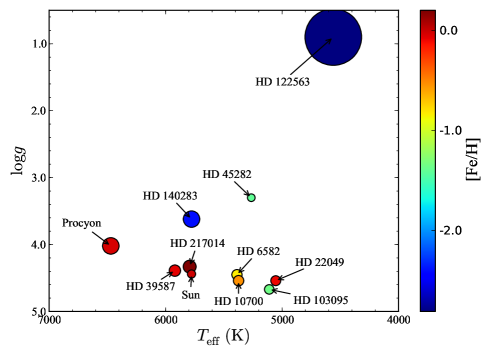
Figure 1: HRD of the program stars. Color encodes metallicity, size encodes stellar diameter measurements.

Interferometric diameter determination for eight of the program stars is available (see Table 1).

To minimize the different instrumental response effects, the spectroscopic parameters ($T_{\rm eff}$, $\log{g}$, [Fe/H] and $\xi$) were taken from Fuhrmann (1998, 2004), who derived them with the same FOCES spectra as we used in this study. The available interferometric observations provide accurate bolometric fluxes (${\cal F}_{\rm BOL}$) with typical uncertainties of $\sim$2% (e.g., Boyajian et al. 2012). Combined with the interferometrically measured stellar angular diameter ($\theta$) measurements with typical relative uncertainties of 1$\sim$3% for our samples, the uncertainties of $T_{\rm eff}=2341({\cal F}_{\rm BOL}/\theta^{2})^{1/4}$ are lower than 1.5%, which is precise enough as cross-validations of the spectroscopic data.

Therefore, whenever possible, we used interferometric $T_{\rm eff}$ and $\theta$ given by recent measurements with VLTI or CHARA to compose interferometric parameters. The spectroscopic and interferometric parameters are summarized in Table 1.

The $\log{g}$ of stars that have interferometric measurements parameters was derived using the direct angular diameter of the star, its distance from the Hipparcos parallax (van Leeuwen 2007), and its mass, either from the astrometric measurements of a binary companion (for Procyon A), or by fitting the stellar evolutionary track in the H-R diagram. The parameters metallicity ([Fe/H]) and micro-turbulence velocity ($\xi$), which cannot be obtained by interferometric means, were kept the same as those in the spectroscopic group. The solar abundance mixture was taken from Lodders et al. (2009). For the five low-metallicity stars in our sample with [Fe/H] ¡ $-$0.60 (HD 6582, [Fe/H] = $-$0.83; HD 103095, [Fe/H] = $-$1.35; HD 122563, [Fe/H] = $-$2.60; HD 45282, [Fe/H] = $-$1.50; and HD 140283, [Fe/H] = $-$2.38), $\alpha$-elements enhancements of [$\alpha$/Fe] = +0.4 were adopted.

A model of Vega was calculated to consistently derive the theoretical zero-point of the spectrophotometric data.

Table 1: Best-fitting $\alpha_{\rm CMA}$

HD	$T_{\rm eff}$ (K)	$\theta_{\rm LD}$	Ref.	$\log{g}$ a	[Fe/H]a	$T_{\rm eff}^{*}$ (K)	The best $\alpha_{\rm CM}$			$\chi^{2}_{\rm red}$(d.o.f)
							Hα	Hβ	Hγ	Hα	Hβ	Hγ
Interferometric and IRFM
Sun	5780$\pm 40$	–		4.44	0.00	5780	2.0	$\geq$1.0	$\geq$1.0	6.05 (244)	–	–
Procyon	6530$\pm 50$	5.448$\pm$0.053	Kervella et al. (2004)	3.98	$-$0.05	6524	1.9	$\geq$1.0	$\geq$1.0	0.94 (309)	–	–
10700	5380$\pm 50$	2.078$\pm$0.031	Di Folco et al. (2004)	4.53	$-$0.49	5330	1.8	$\geq$1.0	$\geq$1.0	0.72 (195)	–	–
103095	4820$\pm 100$	0.679$\pm$0.015	Creevey et al. (2012)	4.59	$-$1.30	5100	2.4	1.9	$\geq$0.5	4.22 (648)	1.84 (217)
39587	5960$\pm 50$	1.051$\pm$0.009	Boyajian et al. (2012)	4.48	$-$0.07	5960	1.9	$\geq$1.0	$\geq$0.5	1.11 (187)	–	–
6582	5260$\pm 85$	0.972$\pm$0.009	Boyajian et al. (2012)	4.51	$-$0.83	5370	1.7	$\geq$0.5	–	0.58 (112)	–	–
217014	5800$\pm 55$	0.748$\pm$0.027	Baines et al. (2008)	4.28	+0.20	5780	2.0	$\geq$1.0	$\geq$1.0	1.08 (236)	–	–
22049	5120$\pm 75$	2.148$\pm$0.029	Di Folco et al. (2004)	4.61	$-$0.09	5045	2.2	$\geq$1.0	–	0.83 (252)	–	–
140283	5780$\pm 50$	–	Casagrande et al. (2010)	3.70	$-$2.38	5780	1.7	1.0	1.0	1.00 (201)	0.60 (547)	1.13 (264)
122563	4600$\pm 50$	0.948$\pm$0.012	Creevey et al. (2012)	1.60	$-$2.60	4600	1.0	0.5	0.5	0.46 (533)	2.50 (236)	2.43 (80)
45282	5300$\pm 50$	–	Casagrande et al. (2010)	3.07	$-$1.50	5310	1.0	0.5	–	0.96 (574)	0.71 (124)	–
Spectroscopic
Procyon	6530	–	This work	3.96	$-$0.05	6530	1.9	$\geq$1.0	$\geq$1.0	–	0.99 (309)	–
103095	5110	–	Fuhrmann (1998)	4.66	$-$1.35	5110	2.4	1.9	$\geq$0.5	–	1.05 (648)	1.07 (217)
39587	5920	–	Fuhrmann (2004)	4.39	$-$0.07	5920	1.5	$\geq$0.5	$\geq$0.5	–	0.96 (187)	–
6582	5390	–	Fuhrmann (2004)	4.45	$-$0.83	5390	2.3	$\geq$1.0	–	0.72 (112)	–	–
217014	5790	–	Fuhrmann (1998)	4.33	+0.20	5790	2.0	$\geq$1.0	$\geq$1.0	0.93 (236)	–	–
22049	5050	–	Fuhrmann (2004)	4.54	$-$0.09	5050	2.2	$\geq$1.0	–	0.80 (252)	–	–

• Notes. ^a References of the adopted $\log{g}$ and [Fe/H] are in the text. $T^{*}_{\rm eff}$ denotes the best effective temperatures obtained from the fitting procedure.

3 Model atmospheres

For each set of stellar parameters, model atmospheres were calculated using the model atmosphere code MAFAGS-OS (Grupp 2004a, b; Grupp et al. 2009). The opacity-sampling (OS) code is based on the opacity distribution function (ODF) version of T. Gehren (1979). In the reprogrammed version of Reile (1987), the code relies on the following basic assumptions:

• Plane-parallel 1D geometry.

• Chemical homogeneity throughout the atmosphere.

• Hydrostatic equilibrium.

• Convection is treated according to the formalism of Canuto & Mazzitelli (1991, 1992).

• No chromosphere or corona.

• Local thermodynamical equilibrium.

• Flux conservation throughout all 80 layers.

While these assumptions can break down for hot stars, stars with very extended atmospheres, and the coolest stars, they are valid for temperatures from 4000 through 15000 K and for gravities from the main sequence down to $\log{g}\approx 0$.

The model was iterated until the flux was constant ($<0.5\%$ level) throughout the atmosphere.

3.1 Convection and atmospheric structure

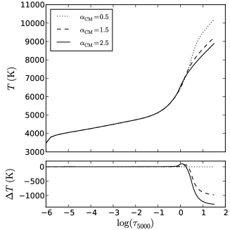
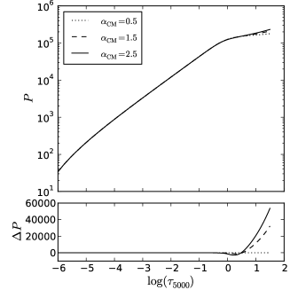
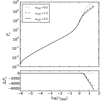
Figure 2: Temperature ($T$), pressure ($P$), and electron pressure ($P_{\rm e}$) versus optical depth $\log(\tau_{5000})$ with three different mixing-length parameters $\alpha_{\rm CMA}$ in the MAFAGS-OS models of Sun.

Figure 2 shows the influence of the convective efficiency parameter $\alpha_{\rm CMA}$ on temperature stratification, gas pressure, and electron pressure of a solar atmospheric model. While a low value of $\alpha_{\rm CMA}$ results in low convective flux, high $\alpha_{\rm CMA}$ leads to an increase of the convective flux and - as the total flux is preserved through all layers - lower radiative flux in the convection zone of the stellar atmosphere. Low radiative flux leads to lower temperature gradients. Therefore, the high-$\alpha_{\rm CMA}$ case shows a lower temperature in the inner region of the stellar atmosphere.

For our program stars, increasing $\alpha_{\rm CMA}$ from 0.5 to 2.5 leads to decreasing temperatures in the inner atmosphere by up to 1000–1300 K at $\log(\tau_{5000})\simeq 1.5$.

The effect of a variation of $\alpha_{\rm CMA}$ on the solar SED is shown in Fig. 3. Flux changes of up to 5% of the solar SED in the UV and of 1% in the near-IR region are notable. There are some node points at 550, 1350, and 2050 nm around which the fluxes are insensitive to mixing-length parameters, while the continuum of the SED between each two shows opposite tendencies with $\alpha_{\rm CMA}$.

The trends in model structures and fluxes are similar for other stars in our sample, with the only exception of the A0V star Vega. As Vega has no convection zone reaching the stellar atmosphere, no change with $\alpha_{\rm CMA}$ is present in the stellar flux.

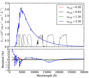
Figure 3: Upper panel: Computed solar flux $F_{\lambda}$ with different $\alpha_{\rm CMA}$. The spectrum is sampled every 50 Å along the wavelength. The transmission curves of U, B, V, R, I in Bessell photometric system, and J, H, K_s in 2MASS system are also overplotted (from left to right). The residuals to fluxes with $\alpha_{\rm CMA}=0.82$ are plotted in the lower panel.

4 Spectral energy distributions

In the following section we directly compare the computed absolute fluxes to the observational data to calibrate $\alpha_{\rm CMA}$. Absolute flux data are only available for a few stars. For our sample, reliable absolute SED data are only available for the Sun and Procyon.

4.1 Near-UV – visible – near-IR domain

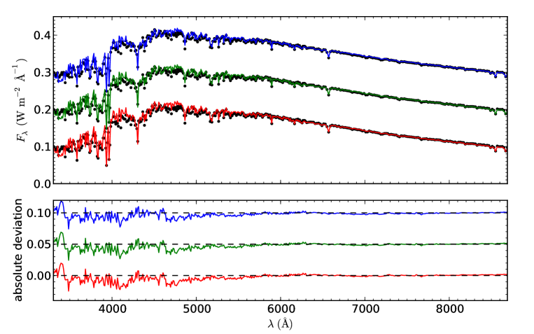
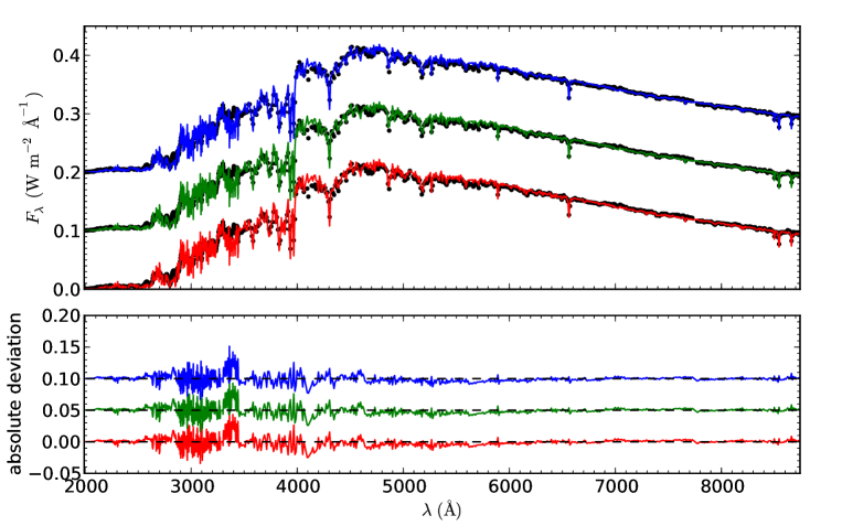
Figure 4: Comparison of solar absolute fluxes (solid dots) to synthetic flux levels with $\alpha_{\rm CMA}=0.5$ (red), 1.5 (green), and 2.5 (blue).
Observational data were taken from Neckel & Labs (1984) (upper panel) and Thuillier et al. (2003) (lower panel). The absolute deviation ($F_{\rm model}-F_{\rm obs}$) is plotted in the lower part of each panel. Offsets of 0.05 were added to improve the visualization.

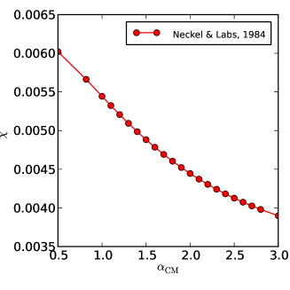
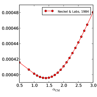
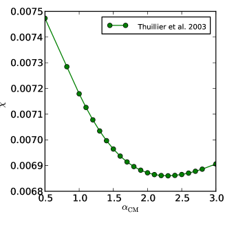
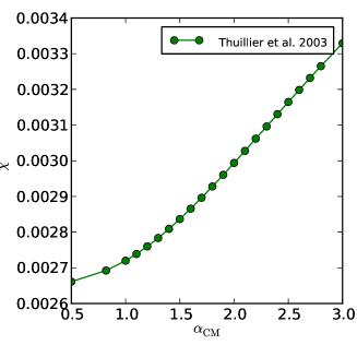
Figure 5: Relations of $\chi^{2}$ of observational and computed fluxes versus $\alpha_{\rm CMA}$ for the solar irradiance of Neckel & Labs (1984) and Thuillier et al. (2003). Observational data between 4500 and 8700 Å (left plots) and between 5500 and 8700 Å (right plots) were taken into account.

Neckel & Labs (1984) measured solar irradiance between 3300 and 12500 Å by combining the absolute fluxes of high-resolution spectra obtained with the Fourier Transform Spectrometer (FTS) at the McMath Solar Telescope on Kitt Peak. The spectra were averaged every 10 Å between 3305 and 6295 Å, and every 20 Å between 6310 and 8690 Å.

Thuillier et al. (2003) presented the solar irradiance from 2000 Å to 24000 Å obtained with the SOLSPEC and SOSP spectrometers mounted on space missions. However, for wavelength ranges above 8700 Å, their data are sampled with a rate different from that in visible and UV domains. Therefore we only adopted the spectra below 8700 Å to compare with our solar fluxes.

Figure 4 shows the data and absolute deviations of solar irradiance of Neckel & Labs (1984) and Thuillier et al. (2003) together with the computed solar fluxes for three different $\alpha_{\rm CMA}$ values of 0.5, 1.5, and 2.5. A visual check prefers a fit between blue ($\alpha_{\rm CMA}=2.5$) and green ($\alpha_{\rm CMA}=1.5$).

The left and right panels of Fig. 5 compare the measured and observed fluxes starting from 4500 Å and 5500 Å. The strong dependency on the blue end of the comparison window does not allow precisely determining $\alpha_{\rm CMA}$ from these data. Nevertheless, data points with values below 1.0 can be excluded from the Neckel data. The data of Thuillier et al. (2003) would only allow for very low convective efficiency if the blue region is ignored. In general, we find an overestimation of the solar flux in the regime below 5000 Å. This can be caused by missing atomic or molecular opacity. Variations of convective efficiency do not change this region significantly, thus can be excluded as the cause of this shortcoming.

4.2 Ultraviolet domain

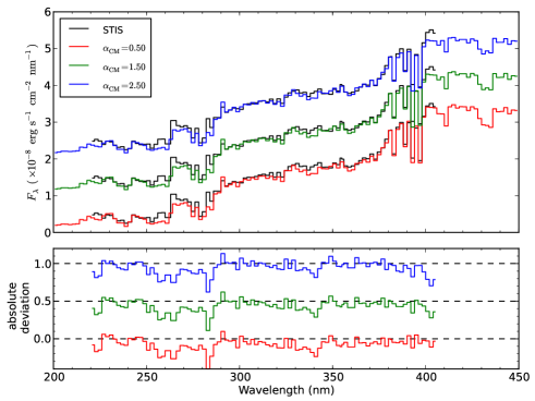
Figure 6: Comparison of absolute fluxes of Procyon A (solid lines) obtained with HST/STIS with MAFAGS-OS model fluxes with $\alpha_{\rm CMA}=0.5$ (red), 1.5 (green), and 2.5 (blue) in model (a). The fluxes were summed every 2 nm. The absolute deviation ($F_{\rm model}-F_{\rm obs}$) were plotted in the lower panel. Offsets of 1.0 in the upper panel and 0.5 in the lower panel were added for clarity.

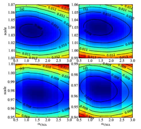
Figure 7: $\chi^{2}$ versus $\alpha_{\rm CMA}$ and the scaling factor for the HST/STIS data and the computed absolute fluxes between 220 and 405 nm with models of different $T_{\rm eff}$ for Procyon A. From (a) to (d): $T_{\rm eff}=6520/6530/6550/6590$ K.

The ultraviolet spectrum of Procyon A has been obtained with the Space Telescope Imaging Spectrograph (STIS) onboard the Hubble Space Telescope (HST) with high-quality calibration in the range from 220 nm up to 405 nm. As the STIS spectra span several echelle orders and overlap between each pair of orders, we averaged bins of 2 nm width for the STIS measured data and MAFAGS-OS model calculations to allow a most direct comparison. This comparison is shown in Fig. 6 for $\alpha_{\rm CMA}$ ranging from 0.5 to 2.5 for a model with a $T_{\rm eff}/\log{g}/$[Fe/H]$/\xi$ = 6530/3.98/$-0.05$/2.10. MAFAGS-OS underestimates the fluxes by at most $\sim$35% for Mg II H & K at 280 nm. The average deviation is within 4%.

Figure 7 displays the 2D plots of $\chi^{2}$ versus $\alpha_{\rm CMA}$ (x axes) and the scaling factor of computed flux (y-axes) for four models with different temperatures. The difference of $\sim 70$ K in $T_{\rm eff}$ causes a difference of $\sim$4% in the total fluxes. The scaling factors were introduced to account for the offsets between the computed fluxes and the observational data to first-order approximation. The relative uncertainty ($\sim 1\%$) of the angular diameter can lead to an offset of up to 2% of the observational SED. Therefore the $\pm 3\%$ of the scaling factor on the total flux is reasonable. The derived $\alpha_{\rm CMA}$ for each model was estimated by minimizing the $\chi^{2}$ with the observational SED over the 2D plane. We found that model (c) and (d) led to smaller $\chi^{2}$ with the observational data, which favors higher $T_{\rm eff}$ for Procyon A. Models (b), (c), and (d) led to quite consistent $\alpha_{\rm CMA}\simeq 1.4$ to minimize $\chi^{2}$, while model (a) favors smaller $\alpha_{\rm CMA}\simeq 1.3$.

5 NLTE calculations of Balmer-line profiles

Our analysis is based on the nonlocal thermodynamical equilibrium (NLTE) line formation for H i using the method described in Mashonkina et al. (2008). In brief, the model atom includes levels with principal quantum numbers up to $n\leq 19$. We checked the influence of inelastic collisions with neutral hydrogen atoms, as computed following Steenbock & Holweger (1984), on the statistical equilibrium (SE) of H i and resulting profiles of the Balmer lines in the models. The differences in normalized fluxes between including and neglecting H+H collisions are smaller than 0.0005 of the continuum flux for the core-to-wing transition region that is most sensitive to $T_{\rm eff}$ variations. Therefore all the NLTE calculations were performed with pure electronic collisions with the exception of a very metal poor (VMP) giant atmosphere 4600/1.60/$-2.6$ and a metal-poor subgiant atmosphere 5777/3.70/$-$2.38, for which S_H=1.0 and 2.0 were adopted.

The coupled radiative transfer and SE equations were solved with a revised version of the code DETAIL (Butler & Giddings 1985). The update was described in Mashonkina et al. (2008). The obtained departure coefficients were then used by the code SIU (Reetz 1991) to calculate the synthetic line profiles. The absorption profiles of Balmer lines were computed by convolving the profiles resulting from the thermal, natural, and Stark broadening, as well as self-broadening. The Stark profile was based on the unified theory as developed by Vidal et al. (1970, 1973, VCS). The calculations of Stehle (1994) based on a different theory agreed reasonably well with the data of VCS. For self-broadening, we applied the Lorentz profile with a half-width computed using the cross-section and velocity parameter from Barklem et al. (2000). As shown by Barklem et al. (2000), ”the complete profiles obtained from overlapping line theory are very closely approximated by the p-d component of the relevant Balmer line”. This gives ground to apply the impact approximation to describe the self-broadening effect on H_α, H_β, and H_γ.

Figure 8: Departure coefficients $\log b_{i}$ for the five lowest levels of H i as a function of continuum optical depth $\tau_{5000}$ referring to $\lambda=5000$Å  in the model atmosphere 6530/3.96/$-0.05$. Tick marks indicate the locations of core-to-wing transition (0.85 to 0.95 in normalized flux) formation depths for H_α and H_β.

We selected the model 6530/3.96/$-0.05$ to show the behavior of the departure coefficients $b_{i}=n_{i}^{\rm NLTE}/n_{i}^{\rm LTE}$ of the relevant levels of H i (Fig. 8). Here, $n_{i}^{\rm NLTE}$ and $n_{i}^{\rm LTE}$ are the SE and thermal (Saha-Boltzmann) number densities, respectively. Very similar behavior of $b_{i}$ was found for all the model atmospheres investigated in this study. The ground state and the $n=2$ level keep their thermodynamic equilibrium level populations throughout the atmosphere. Departures from LTE for the $n=3$ level are controlled by H_α. In the layers where the continuum optical depth drops below unity, H_α serves as the pumping transition, which results in an overpopulation of the upper level. For instance, $b(n=3)\simeq 1.017$ around $\log\tau_{5000}=-0.57$, where the H_α core-to-wing transition is formed. Starting from $\log\tau_{5000}\simeq-2.8$ and farther out, photons that escape from the H_α core cause an underpopulation of the $n=3$ level. For H_α, NLTE leads to a weakening of the core-to-wing transition compared to the LTE case (Fig. 9).

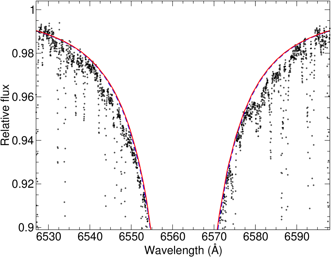
Figure 9: Synthetic NLTE (continuous curve) and LTE (dashed curve) flux profile of H_α computed with the MAFAGS-OS 6530/3.96/$-0.05$ ($\alpha_{\rm CMA}=2.3$) model compared to the observed spectrum of Procyon (bold dots).

To compare them with observations, the computed synthetic profiles were convolved with a profile that combines instrumental broadening with a Gaussian profile of 3.2 km s^-1 to 4.6 km s^-1 for different stars and broadening caused by macroturbulence with a radial-tangential profile of 4 km s^-1. Rotational broadening was only taken into account for Procyon, with $V\sin i$ = 2.6 km s^-1 (Fuhrmann 1998). All the remaining dwarf and subgiant stars were assumed to be slow rotators, with $V\sin i\leq 1$ km s^-1. It is worth noting that the thermal broadening of Balmer lines, with the most probable velocity of about $V_{t}=10$ km s^-1 in the atmospheres of the investigated stars, is more pronounced than the broadening caused by rotation, macroturbulence, and instrumental profile together. Therefore, the uncertainty in the external broadening parameters only has an minor effect on the computed Balmer-line wings.

6 Fitting procedure of Balmer-line wings

Our analysis of H_α is based on profile fitting in the wavelength range from 6473 to 6653 Å  for Procyon and from 6520 to 6608 Å for the remaining stars. We analyzed H_β in the wavelength range 4815 – 4908 Å only for the metal-poor stars HD 103095, HD 122563, HD 45282, and HD 140283. For HD 122563 and HD 140283 we also analyzed H_γ profiles in the wavelength range from 4315 to 4365 Å . Before fitting, we made the following preparations of the observed profiles for all stars.

We excluded the Balmer line cores up to 0.9 of the relative flux (F${}_{i}^{l}$/F${}_{i}^{c}$), because the core half-width of the hydrogen line cannot be described in cool stars with classical model atmospheres. Thus only the pressure-broadened wings were analyzed. As our aim is to fit the profiles of Balmer lines, all blended lines should be removed from the observed profiles. The high resolution of the employed spectra allows us to assume that unblended spectral windows do exist and can be used for the fitting. We identified spectral windows across the line that are expected to be free from blends in the stars of interest. This was done by means of calculating Balmer line profiles with and without metal lines. Then we created a mask that was free from any blends. Based on the examination of the spectra, this is reasonable at H_α for all the reference stars, and at H_β for HD 122563, HD 45282, and HD 140283, and at H_γ only for HD 122563 and HD 140283. It is impracticable to define spectral windows without any blends at H_β and H_γ in solar metallicity stars.

The mask consists of a spectral window of pure H_α, H_β, and H_γ (when available) lines with noise alone. The same mask was applied for all stars, but minor modifications were made for each star individually. Modifications of the mask were necessary to reject stars in some specific cases, for example, if there was an ingress of atmospheric lines in the spectral window or for Procyon, which has much stronger macroturbulence and $V\sin i$ than other stars. It is very important to clearly distinguish between noise fluctuations and weak metal lines in the spectra. In this context, we relied upon the spectral line database and inspected all Balmer line profiles.

We also investigated the effect of spectral resolution on the choice of which spectral windows to mask. It is necessary to have a proper number of spectral windows between blended lines because only by using such a mask are we able to derive the same result regardless of whether we use high-resolution spectra or the spectra degraded to the resolution of our observations. This mask is quite reliable in the case of H_α for all stars, but for H_β and H_γ we were unable to define such a mask for all stars. This makes the results obtained from H_β and H_γ profiles less reliable.

We also took into account the effect of rotational broadening and broadening caused by macroturbulence on the choice of spectral windows of mask. While all our sample stars are slow rotators with $V\sin i\leq 1$ km s^-1 except for Procyon with $V\sin i=2.6$ km s^-1, we were able to find a proper number of spectral windows between blending lines around H_α profiles. In the case of H_β and H_γ profiles, this effect becomes important because there are many blending lines in the two profiles. This prevented us from defining a reliable mask for all stars, except for some metal-poor stars (HD 103095, HD 122563, HD 45282, and HD 140283), which only contain few blending lines in their H_β and H_γ profiles.

In this work we used a method based on a reduced $\chi^{2}$ statistics. Statistical measurement of the goodness-of-fit was performed by comparing the theoretical profile and an observed profile through a $\chi^{2}$ minimization procedure (Nousek & Shue 1989). The estimator of the fit goodness is defined by

$$\chi^{2}_{\rm red}=\frac{1}{n-p-1}\sum_{i=1}^{n}\frac{(O_{i}-C_{i})^{2}}{\sigma_{i}^{2}},$$ (1)

where $O_{i}$ is the relative flux measured at the wavelength $\lambda_{i}$, $C_{i}$ is the relative flux computed from the model at the same wavelength $\lambda_{i}$, $\sigma_{i}$ is the variance of the data point $i$ that is defined as the (S/N)^-1 ratio at the same wavelength $\lambda_{i}$, $n$ is the number of data points, and $p$ is the number of free parameters of the model so that $n-p-1$ is the number of degrees of freedom (d.o.f).

For the spectra of HD 10700 and HD 122563, we did not have the $\sigma_{i}$ at the wavelength $\lambda_{i}$. Although it is known that the S/N depends on the number of recorded photons $I$ ($\sim$ $\sqrt{I}$), we adopted the mean constant S/N ratio for these stars because we only fit the wings of each line up to 0.9 where the S/N ratio is not changed dramatically. For Procyon, for example, the relative flux at a S/N of 0.85 is 10% lower than that with a S/N of 0.995. Apart from the inner wings, which have less strongly blended lines because they are saturated by the hydrogen line, equal weights were assigned for all spectral windows of a line profile.

There were two free parameters, $\alpha_{\rm CMA}$ and the effective temperature, while the other parameters ($\log{g}$, [Fe/H], $\xi$) were fixed. Assuming the Poissonian error distribution, which approaches the normal distribution at high S/N, the minimization of $\chi^{2}$ provides the maximum-likelihood estimate of the parameters, in our case for $\alpha_{\rm CMA}$ and $T_{\rm eff}$.

We also compared a grid of Balmer-line profiles for a given model grid with a 25 K interval in $T_{\rm eff}$ and a 0.1 interval in $\alpha_{\rm CMA}$. By varying the free parameters of the model, we computed the value of $\chi^{2}$ at each step. First we fixed one of the two free parameters, $T_{\rm eff}$, and analyzed the function of $\chi^{2}$, which smoothly changes with varying $\alpha_{\rm CMA}$ and follows an asymmetric parabolic form with one single minimum. The best $\alpha_{\rm CMA}$ and $T_{\rm eff}$ were chosen from the requirement of the lowest $\chi^{2}$ value. The variation of temperature within the error bars allows us to estimate the upper and lower values for our $\alpha_{\rm CMA}$. An example of the fitting for H_α profile in the metal poor star HD 103095 is shown in Fig.10.

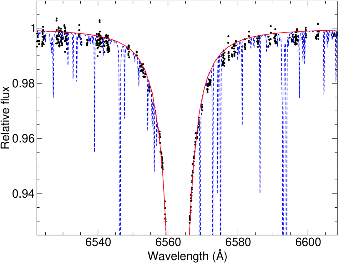
Figure 10: Example of fitting the H_α wings in the metal-poor star HD 103095. Bold dots correspond to the observed data. The theoretical H_α profile was calculated with (dashed curve) and without (solid curve) blending lines. Only bold dots were used for determining the $\chi^{2}$ statistic.

6.1 Errors

Estimated errors are presented in Table 2 for the program stars. The strength of the hydrogen line depends only weakly on the surface gravity or the metallicity. We considered how the typical errors (0.1 dex) for either of them may affect the result. Microturbulence does not affect the formation of the Balmer-line wings (Fuhrmann et al. 1993), therefore we did not consider the influence of microturbulence. Only the temperature can strongly affect the wings of hydrogen lines. With increasing temperature the wings of hydrogen lines tend to be stronger. The effective temperature is the main source of errors in our results. The influence of other sources of error, such as Stark-broadening, self-broadening, and He-broadening, were considered in Fuhrmann et al. (1993, 1994) and Barklem et al. (2002). The latter showed that the influence of Stark- and self-broadening on the behavior of Balmer lines is insignificant for solar metallicity stars, but tends to be stronger for metal-poor atmospheres. Moreover, the determination of the continuum placement is one of the most significant uncertainties in this work. For the sample spectra, the error in the continuum placement of the high-quality spectra is approximately 0.5% of the continuum flux, depending on the S/N ratio. As a result of the interdependency of errors, it is difficult to precisely account for the combined effect, therefore we divided all errors into two groups: those propagated from the stellar parameters ($T_{\rm eff}$, $\log{g}$, and [Fe/H]), and those caused by observational aspects (continuum placement and fitting error).

Table 2: Estimated errors in CMA factor for H_α profiles.

Error	Sun	Procyon	HD 10700	HD 103095	HD 39587	HD 6582	HD 217014	HD 22049	HD 122563	HD 45282	HD 140283
$\Delta T_{\rm eff}$	$\pm 0.2$	$\pm 0.4$	$\pm 0.3$	$\pm 0.3$	$\pm 0.4$	$\pm 0.3$	$\pm 0.3$	$\pm 0.3$	$\pm 0.1$	$\pm 0.3$	$\pm 0.2$
$\Delta\log{g}$ = 0.1 dex	–	–	–	$\pm 0.1$	–	$\pm 0.1$	–	–	$\pm 0.1$	$\pm 0.1$	$\pm 0.1$
$\Delta$[Fe/H] = 0.1 dex	–	$\pm 0.2$	$\pm 0.1$	$\pm 0.1$	–	$\pm 0.1$	$\pm 0.1$	$\pm 0.1$	$\pm 0.1$	–	–
Fitting procedure	$\pm 0.2$	$\pm 0.2$	$\pm 0.1$	$\pm 0.2$	$\pm 0.1$	$\pm 0.5$	$\pm 0.1$	$\pm 0.1$	$\pm 0.2$	$\pm 0.2$	$\pm 0.2$
Continuum
(0.5%)	$\pm 0.3$	$\pm 0.5$	$\pm 0.2$	$\pm 0.3$	$\pm 0.1$	$\pm 0.3$	$\pm 0.1$	$\pm 0.1$	$\pm 0.2$	$\pm 0.2$	$\pm 1.0$
Total	$\pm 0.4$	$\pm 0.7$	$\pm 0.4$	$\pm 0.5$	$\pm 0.4$	$\pm 0.7$	$\pm 0.4$	$\pm 0.4$	$\pm 0.4$	$\pm 0.4$	$\pm 1.1$

7 Results

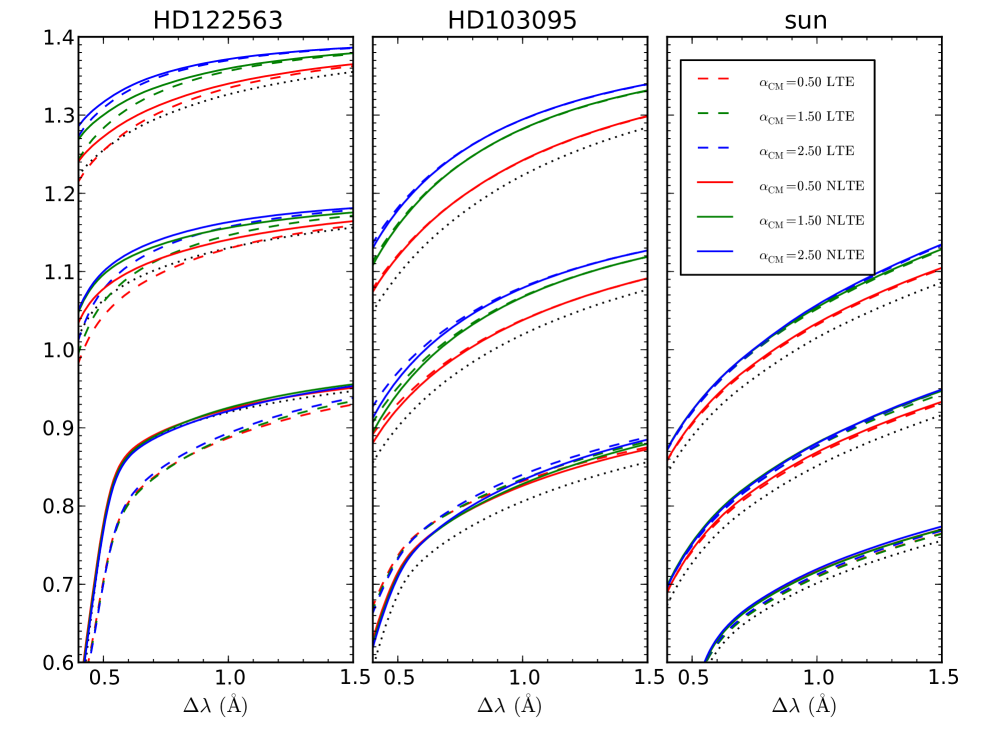
Figure 11: Comparison of the line profiles of H_α, H_β, and H_γ (from bottom to top) for HD 122563, HD 103095, and the Sun. The x-axis is the wavelength shift relative to the center of the Balmer lines. The colors are coded with different $\alpha_{\rm CMA}$ (from 0.5 to 1.5), while the solid lines and dashed lines represent profiles using LTE and NLTE line formations, respectively. The dotted lines are profiles with LTE models of $\alpha_{\rm CMA}=0.5$ but $T_{\rm eff}+100$ K. For clarity, offsets of 0.2 and 0.4 are added to the H_β and H_γ, respectively.

In Fig. 11 we plot the profiles of the Balmer lines for three of our program stars (HD 122563, HD 103095, and the Sun). The profiles are only slightly different under LTE or NLTE assumptions for dwarfs, but exhibit significant variations with $\alpha_{\rm CMA}$ on their wings. The changes with $\alpha_{\rm CMA}$ from 0.5 to 2.5 are similar (for H_α) and even larger (for H_β and H_γ) to that of $T_{\rm eff}$ of a few hundreds of Kelvin. For the metal-poor giant HD 122563, the NLTE effect plays a more important role than $\alpha_{\rm CMA}$ for H_α profile, but is less sensitive than $\alpha_{\rm CMA}$ parameter. Figure 11 also indicates that if the $\alpha_{\rm CMA}$ parameter in the model atmosphere is not correct, the $T_{\rm eff}$ may be biased by up to a few hundreds of Kelvin by fitting H_β or H_γ line profiles. Therefore, caution must be exercised when choosing $\alpha_{\rm CMA}$ in 1D model atmospheres.

7.1 The Sun

The Sun is the best-known star with high-quality observations and accurate physical parameters. Following Fuhrmann et al. (1993), we attempted to calibrate $\alpha_{\rm CMA}$ for the solar atmosphere. Our work differs from that of Fuhrmann et al. (1993) in that we have used the self-broadening theory of Barklem et al. (2000). For investigations of the Sun we employed the solar atlas (Kurucz et al. 1984). We adopted an effective temperature of 5777 K with an error bar of $\pm$40 K. By fitting theoretical H_α profiles to reduced observational profiles, the two parameters $T_{\rm eff}$ and $\alpha_{\rm CMA}$ were varied within error bars and reasonable physical limits, respectively. The results are shown in Fig. 12, where the $\chi^{2}$ minimum indicates the best $T_{\rm eff}$ and $\alpha_{\rm CMA}$.

Figure 13 compares the left wing of H_α line profile for the Sun with the theoretical spectrum for $\alpha_{\rm CMA}=2.0$ (solid line).

The combination of $T_{\rm eff}$=5770$\pm 20$ K and $\alpha_{\rm CMA}=2.0\pm 0.2$ is preferred based on the degree of agreement between the observational and theoretical H_α profiles. Nevertheless, it is important to note that the value of $\chi^{2}$ is still high, which suggests that our agreement between the observational and the theoretical H_α profiles is not perfect. This means that the quality of the observed solar flux spectra is higher than the quality of theoretical surveys.

From comparison with SED, a low value for $\alpha_{\rm CMA}<1.0$ is excluded. The lack of fitting in the region below 5000 Å does not allow precisely determining the convective efficiency, but the measurements are consistent with an $\alpha_{\rm CMA}$ of 2.0.

7.2 Procyon

Procyon (HD 61421, HR 2943) is one of the brightest stars in the night sky ($V=0.34$). It is a binary system consisting of an F5 IV-V star (Procyon A) with a mass of $1.497\pm 0.037\ M_{\odot}$ and a faint white dwarf (Procyon B) with a mass of $0.602\pm 0.015\ M_{\odot}$, orbiting each other with a period of 40.8 years (Girard et al. 2000). Spectroscopic analyses gave rather discrepant effective temperatures, from 6470 K (by fitting the Balmer lines; Zhao & Gehren 2000) to 6850 K (by measuring the equivalent widths of a large set of iron lines; Heiter & Luck 2003). The proximity of Procyon ($\pi=284.56\pm 1.26$ mas; van Leeuwen 2007) to the Earth allows us to directly measure its angular diameter (e.g., Hanbury Brown et al. 1974; Mozurkewich et al. 1991; Aufdenberg et al. 2005; Chiavassa et al. 2012). Kervella et al. (2004) found $T_{\rm eff}=6530\pm 50$ K and $\log{g}=3.96\pm 0.2$, which agrees well with other works (e.g., Allende Prieto et al. 2002; Fuhrmann et al. 1997). We used a high-quality spectrum of H_α for Procyon and applied the same fitting method as described in the previous sections.

The results are displayed in Fig. 12, where the $\chi^{2}$ minimum indicates the best $T_{\rm eff}$ and $\alpha_{\rm CMA}$. For this star we find $T_{\rm eff}=6524\pm 50$ K and $\alpha_{\rm CMA}=1.9\pm 0.7$. The error of $\alpha_{\rm CMA}$ is not symmetric in this case, but we adopted the largest. The left wing of the H_α line profile for Procyon is shown in Fig. 13, where two theoretical spectra with $\alpha_{\rm CMA}=1.5$ (solid line) and $\alpha_{\rm CMA}=2.3$ (dashed line) are plotted as well.

The value preferred from the SED fitting for $\alpha_{\rm CMA}\approx 1.4$, nevertheless, there are large uncertainties with respect to opacity data. As a result of the uncertain UV flux comparison, the values given by SED fitting and that by Balmer profiles do not contradict each other.

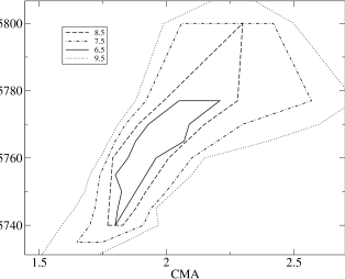
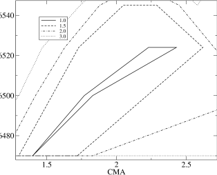
Figure 12: Survey of the reduced $\chi^{2}$ obtained from H_α profile fitting for the observed solar flux spectra (top panel) and spectra of Procyon (bottom panel) with different $\alpha_{\rm CMA}$ and $T_{\rm eff}$. The preferred parameter area is located where $\chi^{2}$ is minimal. All $\chi^{2}$ are not normalized and indicate a good fit in each case.

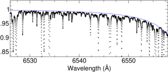
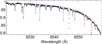
Figure 13: Left wings of H_α line profiles for the Sun with $\alpha_{\rm CMA}=2.0$ (top panel) and Procyon (bottom panel), where two theoretical spectra with $\alpha_{\rm CMA}=1.5$ (solid line) and $\alpha_{\rm CMA}=2.3$ (dash line) are shown.

7.3 Program stars

The final results of our fitting are given in Table 1, including the names of the program stars, their parameters, the best $\alpha_{\rm CMA}$ along with the limits, and the $\chi^{2}$ values that indicate the best fit in each case. We also present the best-fit $T_{\rm eff}$ within the error bars that was obtained during the $\chi^{2}$ minimization procedure. Temperatures with asterisks are the best-fit temperatures. The results from H_β and H_γ for some stars are less reliable. Even though good-quality observations of H_β and H_γ are available for all remaining stars, these lines were not adopted because choosing a reliable mask was problematic.

The observed spectra and the best-fitting line profiles from this method are plotted in Fig. 14. When applying the above-mentioned method, we have to keep in mind that weak blending lines may, nevertheless, be presented in a chosen windows. Therefore, it would be better to inspect the best profiles visually to give preference to the case where all observed points are below the theoretical line profile, but the $\chi^{2}$ – method minimizes the deviations without considering whether the observed points are above or below the theoretical profile. In this context, for the $\chi^{2}$ method, $\alpha_{\rm CMA}$ will be slightly underestimated, while the best-fit $T_{\rm eff}$ will be overestimated.

The derived $T_{\rm eff}$ for stars HD 10700, HD 39587, HD 217014, HD 22049, HD 122563, HD 45282, and HD 140283 agree well with those derived from astrometric and IRFM methods. However, for HD 103095 we were unable to find an appropriate $T_{\rm eff}$ in the temperature range $T_{\rm eff}=4820\pm 100$ K. Thus, for this star we adopted a higher spectroscopic temperature of $T_{\rm eff}=5110$ K.

Figure 14: Best fits of the H_α lines in our stellar sample. Solid lines are the theoretical spectra corresponding to the best fit and dotted lines represent the observed spectra that were used for determining the $\chi^{2}$ statistic. The horizontal dotted lines show the limit of reasonableness of the approximation and allows seeing residuals.

The individual results for our stellar sample are reported below.

HD 6582 ($\mu$ Cas, 30 Cas, HR 321) is a close binary system that consists of a slightly metal-deficient subdwarf (component A, $V=5.17$) and a component B fainter by 5.3 magnitudes ($V=10.5$), with a separation of only 0”.40$\sim$1”.40 (Mason et al. 2001). The spectroscopic parameters adopted here for HD 6582 A ($T_{\rm eff}=5387$ K, $\log{g}=4.45$, [Fe/H] = $-0.83$, and $\xi=0.89$ km s^-1) were taken from Fuhrmann (2004). Boyajian et al. (2012) measured its limb-darkened angular diameter $\theta_{\rm LD}=0.972\pm 0.009$ mas with CHARA, corresponding to the stellar radius of $0.790\pm 0.009\,R_{\odot}$, combining with the Hipparcos parallax ($\pi=132.38\pm 0.82$ mas; van Leeuwen 2007). This is agrees well with the spectroscopic radius ($R=0.8\,R_{\odot}$), but the interferometric $T_{\rm eff}=5264$ K is $\sim$120 K lower than that of Fuhrmann (2004). By comparing the H_α profile, we found the best $\alpha_{\rm CMA}=2.3$ for spectroscopic parameters, while $\alpha_{\rm CMA}=1.7$ for interferometric parameters. Despite this large discrepancy, the fitting method with the interferometric model (b) led to lower $\chi^{2}$ and supports a higher $T_{\rm eff}=5370$ K. This result supports the relative high $T_{\rm eff}$ of 5339 K derived by the photometric $b-y=0.437$ and $c_{1}=0.213$ (Hauck & Mermilliod 1998) with the color-$T_{\rm eff}$ relation of Alonso et al. (1996).

HD 10700 ($\tau$ Cet, 52 Cet, HR 509) is a nearby and inactive G8 V star, with a distance of only $3.650\pm 0.002$ pc ($\pi=273.96\pm 0.17$ mas; van Leeuwen 2007). It is one of the most frequently observed targets in several precise radial velocity surveys for extrasolar planets, and Tuomi et al. (2013) reported five planets with minimum masses of up to 6.6 $M_{\oplus}$ orbiting it. Spectroscopic analyses indicate that its $T_{\rm eff}$ ranges from 5283 K (Valenti & Fischer 2005) to 5420 K (Takeda et al. 2005), and [Fe/H] range from $-$0.43 (Takeda et al. 2005) to $-$0.58 (Luck & Heiter 2005). Interferometric measurements with VLTI gave $\theta_{\rm LD}=2.078\pm 0.031$ mas (Di Folco et al. 2004), and $T_{\rm eff}$ was perfectly consistent with the spectroscopic parameters ($T_{\rm eff}=5377$ K, $\log{g}=4.53$, [Fe/H] = $-0.49$, and $\xi=0.8$ km s^-1; Mashonkina et al. 2011). With a least $\chi^{2}$ fitting, we found the best $\alpha_{\rm CMA}=1.8$, and the best $T_{\rm eff}=5330$ K agrees with the $T_{\rm eff}=5346$ K inferred from the $b-y$ and $c_{1}$ color (Hauck & Mermilliod 1998; Alonso et al. 1996).

HD 22049 ($\epsilon$ Eri, 18 Eri, HR 1084) is a nearby ($\pi=310.94\pm 0.16$ mas; van Leeuwen 2007), chromospherically active K2 V star orbited by a dusty ring (Greaves et al. 1998). Atmospheric parameter determinations based on high-resolution spectra gave very consistent results, with a $T_{\rm eff}$ ranging from 5054 K (Fuhrmann 2004) to 5200 K (Luck & Heiter 2005), $\log{g}$ ranging from 4.40 (Mishenina et al. 2013) to 4.72 (Takeda et al. 2005), and [Fe/H] ranging from $-0.18$ (Ghezzi et al. 2010) to +0.06 (Takeda et al. 2005). We adopted the parameters of Fuhrmann (2004) ($T_{\rm eff}$ = 5054 K, $\log{g}$ = 4.54, [Fe/H] = $-$0.09, and $\xi$ = 0.9 km s^-1). Di Folco et al. (2004) suggested an interferometric angular diameter of $\theta_{\rm LD}=2.148\pm 0.029$ mas and an effective temperature of $T_{\rm eff}=5122$ K. H_α profile fitting with spectroscopic and interferometric methods result in quite consistent $\alpha_{\rm CMA}=2.2$. The best-fit $T_{\rm eff}=5045$ K also agrees with the photometric $T_{\rm eff}=5074$ K from the $b-y$ and $c_{1}$ (Hauck & Mermilliod 1998).

HD 39587 ($\chi^{1}$ Ori, 54 Ori, HR 2047) is a variable star of RS CVn type, orbiting by a faint ($V_{\rm A}$ = 4.4, $V_{\rm B}=8.8$) companion with a mass of $0.15\pm 0.01\ M_{\odot}$ (Irwin et al. 1992). Boyajian et al. (2012) measured its angular diameter $\theta_{\rm LD}=1.051\pm 0.009$ mas with a precision of 0.9%. This yield a radius of $0.979\pm 0.009\ R_{\odot}$ with a Hipparcos parallax of $115.43\pm 0.27$ mas (van Leeuwen 2007). Boyajian et al. (2012) also gave its effective temperature as $T_{\rm eff}=5961$ K, which generally agrees with the spectroscopic temperature reported by Fuhrmann (2004). We found the best-fit $\alpha_{\rm CMA}=1.5$ for spectroscopic parameters and $\alpha_{\rm CMA}=1.9$ for interferometric parameters.

HD 122563 (HR 5270) is the most metal-poor halo star ([Fe/H]$\sim-2.6$) that can be seen by the naked eye ($V=6.2$) in the night sky. It is the only giant in our program stars and therefore provides unique constraints. Mashonkina et al. (2011) presented a detailed analysis of the NLTE formation of iron lines for this star, and we used the same parameters ($T_{\rm eff}=4600$ K, $\log{g}=1.60$, [Fe/H] = $-$2.60, and $\xi$ = 1.95 km s^-1). Recent interferometric measurements with CHARA and PTI (Creevey et al. 2012) gave its angular diameter as $\theta_{\rm LD}=0.948\pm 0.012$ mas, and $T_{\rm eff}=4598\pm 41$ K, which is consistent with its spectroscopic temperature. We found the best-fit $\alpha_{\rm CMA}=1.0$ with H_α profile, while the fitting of H_β and H_γ gave satisfactory agreement with $\alpha_{\rm CMA}=0.5$. The $\alpha_{\rm CMA}$ is lower than that of the dwarfs, implying that the stellar convective energy transport become less efficient after stars evolved off the main sequence.

HD 217014 (51 Peg, HR 8729) is a nearby ($\pi=64.07\pm 0.38$ mass; van Leeuwen 2007) G5 V star with the first extrasolar planet ever discovered orbiting a Sun-like host (Mayor & Queloz 1995). Spectroscopic analysis gave its effective temperatures as ranging from 5710 K (Maldonado et al. 2012) to 5832 K (Ramírez et al. 2009). The narrow-band photometric color indices $b-y=0.416$ and $c_{1}=0.371$ (Hauck & Mermilliod 1998) indicate a rather low $T_{\rm eff}=5661$ K (Alonso et al. 1996). The parameters adopted here ($T_{\rm eff}=5793$ K, $\log{g}=4.33$, [Fe/H] = +0.20, and $\xi$ = 0.95 km s^-1, Fuhrmann 1998) agree for the effective temperature with the interferometric results of $T_{\rm eff}=5804$ K and $\theta_{\rm LD}=0.748\pm 0.027$ mas (Baines et al. 2008). We found a best-fit of $\alpha_{\rm CMA}=2.0$ with both parameters giving consistent results.

HD 45282 is a G 0 metal-poor star ([Fe/H] $=-1.5$) at low Galactic latitude ($b=-3.9^{\circ}$). Previous spectroscopic analyses gave its $T_{\rm eff}$ as ranging from 5150 K (Fulbright 2000) to 5344 K (Gratton et al. 2000). Considering its high reddening with $E(B-V)\simeq 0.82$ at this direction (Schlegel et al. 1998), we used the IRFM $T_{\rm eff}$ from Casagrande et al. (2010), which is thought to be less affected by interstellar medium. The Balmer profile $\chi^{2}$ fitting gives $\alpha_{\rm CMA}=0.1$ for H_α and $\alpha_{\rm CMA}=0.5$ for H_β with the best-fit $T_{\rm eff}=5310$ K. The error of 0.05 on $E(B-V)$ causes an uncertainty of $\sim 300$ K on $T_{\rm eff}$, therefore the photometric temperature is not reliable.

For the Sun we used the widely adopted parameters of $T_{\rm eff}=5777$ K, $\log{g}=4.44$, [Fe/H] = 0.0, and $\xi=0.90$ km s^-1 and for Vega $T_{\rm eff}=9550$ K, $\log{g}=3.95$, [Fe/H] = $-0.50$, and $\xi=2.00$ km s^-1 (Castelli & Kurucz 1994). The solar $\alpha_{\rm CMA}$ from the H_α Balmer line is 2.0, while a determination based on the solar flux suggests a value of 1.5–1.75. Although this is consistent within the error bars, it has to be noted that, for both the Sun and Procyon, SED fitting leads to a notably lower value of $\alpha_{\rm CMA}$ than Balmer-line fitting.

7.4 $\alpha_{\rm CMA}$

Figure 15: Determined $\alpha_{\rm CMA}$ for the program stars. An error of $\alpha_{\rm CMA}$ of $\approx\pm 0.4\dots 0.7$ maybe assumed for all stars except HD140283 ($T_{\rm eff}=5780$ K, $\log{g}=3.70$ where the error reaches $\approx\pm 1.1$.

Figure 15 shows our final results for the efficiency parameter $\alpha_{\rm CMA}$ as determined from Balmer-line fitting. Except for evolved stars, $\alpha_{\rm CMA}$ is consistent with a value of about 2.0 for all objects within the given insecurities. There is no obvious correlation with metallicity and a weak trend of increasing $\alpha$ for the coolest main-sequence objects in the investigated range of F- and G-type stars. This confirms the behavior and numerical values predicted by Magic et al. (2014) for this part of the HRD.

For the evolved stars of our sample $\alpha_{\rm CMA}$ is of about 1.0. Although Magic et al. (2014) predicted the same trend of lower convective efficiency for objects with lower $\log{g}$, the magnitude of the change is much greater in our sample than that suggested by the 3D simulation of Magic et al. (2014). Our sample mainly consists of main-sequence stars and only contains three evolved objects with well-determined parameters. Nevertheless, the stars clearly show a behavior different from that suggested by Magic et al. (2014). The three objects span a wide range of temperatures, therefore the evolutionary state seems to be the main discriminator that separates them from the rest of the sample.

8 Discussion and implication

Figure 16 shows the difference between the suggested $\alpha_{\rm CMA}$ and that from Magic et al. (2014), who adopted a calibration using the entropy jump (Fig. 3 in their work). As described above, the differences are small along the main sequence and increase dramatically later in the evolutionary sequence, which suggests that there is either a stronger variation of $\alpha_{\rm CMA}$ as predicted by the STAGGER grid, or that our modeling of the Balmer lines is incorrect. The latter is excluded because we generally determined a temperature that agreed well with astrometric and IRFM data.

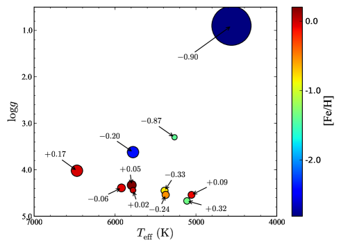
Figure 16: Difference between our determined $\alpha_{\rm CMA}$ and the one predicted by Magic et al. (2014).

Based on the similar method of FAG93, our analysis indicates that if the theory of Barklem et al. (2000) for Balmer-line broadening is adopted instead of that of Vidal et al. (1970, 1973), while the old ODF version is replaced by the MAFAGS-OS version, it is very unlikely to derive a low value of $\alpha_{\rm CMA}=0.82$. For F- and G-type main-sequence stars, $\alpha_{\rm CMA}\approx 2.0$ is derived, and the value decreases toward 1.0 for more evolved stars.

A variation of the convective efficiency naturally influences the temperatures determined by the Balmer-line method. It furthermore changes stellar SEDs and in turn filter fluxes and color determinations. All stellar lines that have contribution functions down to the convection scone (very strong lines) are subject to potential changes as well.