Solving the inhomogeneous Bethe-Salpeter Equation in Minkowski space: the zero-energy limit

Abstract

For the first time, the inhomogeneous Bethe-Salpeter Equation for an interacting system, composed by two massive scalars exchanging a massive scalar, is numerically investigated in ladder approximation, directly in Minkowski space, by using an approach based on the Nakanishi integral representation. In this paper, the limiting case of zero-energy states is considered, extending the approach successfully applied to bound states. The numerical values of scattering lengths, are calculated for several values of the Yukawa coupling constant, by using two different integral equations that stem within the Nakanishi framework. Those low-energy observables are compared with (i) the analogous quantities recently obtained in literature, within a totally different framework and (ii) the non relativistic evaluations, for illustrating the relevance of a non perturbative, genuine field theoretical treatment in Minkowski space, even in the low-energy regime. Moreover, dynamical functions, like the Nakanishi weight functions and the distorted part of the zero-energy Light-front wave functions are also presented. Interestingly, a highly non trivial issue related to the abrupt change in the width of the support of the Nakanishi weight function, when the zero-energy limit is approached, is elucidated, ensuring a sound basis to the forthcoming evaluation of phase-shifts.

1 Introduction

Within a field theoretical framework, it is a highly non trivial challenge to develop non perturbative tools in Minkowski space, but it is quite desirable to devote efforts in that direction, in order to gain insights that could turn out useful in particle physics. In the last few years, solving the homogeneous Bethe-Salpeter equation (BSE) SB_PR84_51 , directly in Minkowski space, has made a substantial step forward KWa ; KWb ; carbonell1 ; carbonell2 ; carbonell3 ; carbonell4 ; carbonell5 ; FSV1 ; FSV2 ; FSV3 due to approaches based on the so-called Nakanishi perturbation-theory integral representation (PTIR) of the $n$-leg transition amplitudes nak71 .

The Nakanishi PTIR for the three-leg amplitude is emerging as a very effective tool for studying the bound state problem KWa ; KWb ; carbonell1 ; carbonell2 ; carbonell3 ; carbonell4 ; carbonell5 ; FSV2 ; FSV3 , within a rigorous field-theory framework. Though the Nakanishi PTIR of the three-leg amplitude, or vertex function, had been devised within the perturbative framework of the Feynman diagrams (as it happens for any $n$-leg amplitude PTIR), it has been shown to work extremely well as the initial Ansatz for obtaining actual solutions of the homogeneous BSE. It must be recalled that BSE, being an integral equation, belongs to a non perturbative realm, and therefore the Nakanishi integral representation of the three-leg amplitude can be only an Ansatz, when exploited in this context.

The main features of the Nakanishi integral representation of any $n$-leg amplitude are basically related to the formal infinite sum of the parametric Feynman diagrams, that contribute to the amplitude under consideration. In particular, the $n$-leg amplitude PTIR has a well-defined structure, given by the folding of (i) a denominator, containing all the allowed independent invariants and governing the analytic behavior of the amplitude itself, and (ii) a weight function, that is a real function depending upon real variables (one is a non compact variable, while the others are compact). It should be emphasized that, at this stage, the Nakanishi weight function has only a formal expression nak71 . If there were an equation for explicitly determining such a weight function, then one could quantitatively evaluate the actual $n$-leg amplitude, under consideration. The homogeneous BSE, that obviously does not belong to the original framework of PTIR, has inspired a different usage of the formal expression of a particular $n$-leg amplitude, namely the three-leg one, or vertex function. Indeed, if one assumes that the Nakanishi integral representation of the three-leg amplitude be formally valid also for the BS amplitude (still a three-leg amplitude, but for a bound state), then the weight function could be considered as an unknown function to be determined. It has to be pointed out that, a priori, there is no guarantee that such an approach for solving BSE be successful, given the caveat above mentioned. Fortunately, it works, as shown in Refs. KWa ; KWb ; carbonell1 ; carbonell2 ; carbonell3 ; carbonell4 ; carbonell5 ; FSV2 ; FSV3 , where the above strategy was applied, but with some differences, for solving the homogeneous BSE directly in Minkowski space. More precisely, by using the PTIR Ansatz for the BS amplitude one can derive, in a formally exact way, an equation for the Nakanishi weight function, starting from the homogeneous BSE, and look for solutions. If the new equation for the weight function has solution, then one can claim that BS amplitudes, actual solutions of the homogeneous BSE in Minkowski space, can be (i) formally written like the PTIR three-leg amplitude, and (ii) numerically determined. In order to achieve a formally exact integral equation for the weight function from BSE, it is very useful and effective adopting a Light-front (LF) framework. This has been done both in the covariant version of the LF framework carbonell1 and in the non-explicitly covariant one FSV1 . In particular, the bound states of a massive two-scalar system interacting through the exchange of a massive scalar have been studied by adopting both ladder carbonell1 ; carbonell3 ; carbonell4 ; FSV2 ; FSV3 and cross-ladder approximations of the BS kernel carbonell2 . Notably, the extension to a bound fermionic system have been also undertaken carbonell5 . It has to be recalled that numerical investigations of the homogeneous BSE has been performed also by considering the standard 4-dimensional variables KWa ; KWb .

The successful achievements for the homogeneous BSE encourage the extension of the Nakanishi integral representation to the study of the inhomogeneous BSE, i.e. the integral equation that determines the scattering states. Our aim is to present a new application of our general approach FSV1 , based on the so-called LF projection of the BS amplitude, i.e. the exact integration on the minus component of the relative four-momentum that appears in the BS amplitude. After applying this formally exact step to BSE, we have numerically investigated the zero-energy limit of the inhomogeneous BSE, for a massive two-scalar system interacting through the exchange of a massive scalar, in ladder approximation. The calculated scattering lengths have been compared in great detail with the analogous observables recently obtained carbonell6 ; carbonell7 within a completely different framework. We have also compared our results with the non relativistic scattering lengths, with the intent to yield a possible guidance for lowering the model dependence in the treatment of interacting final states, pertaining to relevant hadronic decay modes. Indeed, improving and widening our study could contribute to achieve an actual evaluation of the covariant off-shell T-matrix, that represents a key ingredient for describing, e.g., the heavy meson decay amplitudes, like in $D\to K\pi\pi$ processes MagPRD11 ; GuiJHEP14 , and could also have an impact in the development of final-state-interaction models, needed in the analysis of the CP violation in charmless three-body $B$ decays BedPRD14 . Moreover, we have properly analyzed the distorted part of the zero-energy wave function, putting in evidence the relation between a non smooth behavior of the Nakanishi weight function and the expected singularities of the LF 3D wave function, like the one that brings the information relative to the global propagation of the interacting two-scalar system. Finally, the integral equation for the Nakanishi weight function obtained by applying the so-called uniqueness theorem nak71 , is carefully analyzed for the general case of positive energy. Such an in-depth analysis allows us to illustrate a surprising change in the width (from $(-\infty,\infty)$ to $[0,\infty)$) of the support of the Nakanishi weight function with respect to its non compact variable, when the zero-energy limit is considered. Clarifying this feature allows us to put the forthcoming calculation of the phase-shifts on a sound basis, since their calculation requests a careful analysis from both the theoretical and numerical points of view, as it will be illustrated elsewhere FSV4 . By concluding this Introduction, it could be useful to remind that developing genuine non perturbative descriptions of the scattering processes within the Minkowski space, possibly applying formally exact frameworks, is an appealing goal, in view of attempts of extracting tiny, but fundamental signals once very accurate experimental data will become available.

The paper is organized as follows. In Sec. 2, we shortly introduce both the definitions and the general formalism, and we thoroughly discuss the problem of the support of the Nakanishi weight function, given its relevance for the zero-energy limit. Sec. 3 illustrates how to evaluate the scattering length from the Nakanishi weight function, in ladder approximation. In Sec. 4, the numerical studies of the scattering length are presented and compared with the existing calculations found in literature; moreover the scattering 3D LF wave function (indeed the distorted part) is analyzed. Finally, in Sec. 5, the conclusions are drawn.

2 The Nakanishi Integral Equations for scattering states

In this Section, (i) we quickly recall the general formalism of Ref. FSV1 , for obtaining two integral equations that allows one to determine the Nakanishi weight function needed for scattering processes, and (ii) we demonstrate a relevant feature of the weight-function support, that it turns out to be very important also for numerically solving the inhomogeneous BSE.

In our investigation, we considered an interacting system composed by two massive scalars that exchange a massive scalar. This is a generalization of the honorable Wick-Cutkosky modelGW ; Cut in two respects: (i) the interaction takes place through a massive-scalar exchange and (ii) the scattering states is our focus.

2.1 General formalism

For scattering states, the incoming particles are on their-own mass-shell and we indicate their total and relative four-momenta with $p$ and $k_{i}$, respectively. By assuming that the inhomogeneous BS amplitude $\Phi^{+}(k,p,k_{i})$ be expressed in terms of the Nakanishi weight-function $g^{(+)}(\gamma^{\prime},z^{\prime},z^{\prime\prime};\kappa^{2},z_{i})$, then one can write (cf Ref. FSV1 )

$$\Phi^{(+)}(k,p,k_{i})=$$

$$=(2\pi)^{4}\delta^{(4)}(k-k_{i})-i~{}\int_{-1}^{1}dz^{\prime}\int_{-1}^{1}dz^{\prime\prime}\int_{-\infty}^{\infty}d\gamma^{\prime}$$

$$\times\frac{g^{(+)}(\gamma^{\prime},z^{\prime},z^{\prime\prime};\kappa^{2},z_{i})}{\left[\gamma^{\prime}+m^{2}-\frac{1}{4}M^{2}-k^{2}-p\cdot k\;z^{\prime\prime}-2k\cdot k_{i}~{}z^{\prime}-i\epsilon\right]^{3}}=$$

$$=(2\pi)^{4}\delta^{(4)}(k-k_{i})-i~{}\int_{-1}^{1}dz^{\prime}\int_{-1}^{1}dz^{\prime\prime}\int_{-\infty}^{\infty}d\gamma^{\prime}~{}\times$$

$$\frac{g^{(+)}(\gamma^{\prime},z^{\prime},z^{\prime\prime};\kappa^{2},z_{i})}{\left[{\cal D}_{0}-i\epsilon\right]^{3}}\,,$$ (1)

where the total four-momentum is $p\equiv\{M,{\bf 0}\}$ and

$${\cal D}_{0}=\gamma^{\prime}+\gamma+\kappa^{2}-k^{-}(k^{+}+{M\over 2}z^{\prime\prime}-{M\over 2}z_{i}z^{\prime})$$

$$-k^{+}{M\over 2}(z^{\prime\prime}+z_{i}z^{\prime})+2z^{\prime}cos\varphi\sqrt{\gamma\gamma_{i}}~{}~{}.$$

The power of the denominator is the same one adopted for describing a bound state (cf Refs. carbonell1 ; carbonell2 ; FSV1 ; FSV2 ; FSV3 ). Exploiting a standard formalism introduced in Ref. carbonell1 , one defines $z_{i}=-2k^{+}_{i}/M$ and gets $z_{i}=2k^{-}_{i}/M$, since the incoming particles are on their-own mass shell: $(p/2\pm k_{i})^{2}=m^{2}$. Moreover, one has $1\geq|z_{i}|$, since the incoming particles have positive longitudinal momenta, i.e. $p^{+}/2\pm k^{+}_{i}\geq 0$. In Eq. (1), the following notations have been used: (i) $cos\varphi=\widehat{\bf k}_{\perp}\cdot\widehat{\bf k}_{i\perp}$, (ii) $\gamma=|{\bf k}_{\perp}|^{2}$ and $\gamma_{i}=|{\bf k}_{i\perp}|^{2}$, and (iii) $\kappa^{2}=m^{2}-M^{2}/4$. For the initial state one has

$$(p/2\pm k_{i})^{2}=m^{2}={M^{2}\over 4}+k^{+}_{i}k^{-}_{i}-\gamma_{i}=(1-z^{2}_{i}){M^{2}\over 4}-\gamma_{i}\,,$$ (2)

with necessarily $(z_{i})^{2}<1$. Hence one gets

$$M^{2}=4~{}{(m^{2}+\gamma_{i})\over(1-z^{2}_{i})}$$

$$\kappa^{2}=-\gamma_{i}-z^{2}_{i}{M^{2}\over 4}=k^{2}_{i}~{}\leq~{}0\,,$$ (3)

To complete the generalities, we also give the expression for the inhomogeneous BSE, without self-energy insertions and vertex corrections, in the present stage of our approach,. Then, one can write

$$\Phi^{(+)}(k,p,k_{i})=(2\pi)^{4}\delta^{(4)}(k-k_{i})$$

$$+G_{0}^{(12)}(k,p)~{}\int\frac{d^{4}k^{\prime}}{(2\pi)^{4}}i~{}{\cal K}(k,k^{\prime},p)\Phi^{(+)}(k^{\prime},p,k_{i})\,,$$ (4)

where $i~{}{\cal K}$ is the interaction kernel (where the vertex corrections should appear), and $G_{0}^{(12)}$ is the free two-particle Green’s function given by

$$G_{0}^{(12)}(k,p)=G_{0}^{(1)}G_{0}^{(2)}=$$

$$=\frac{i}{(\frac{p}{2}+k)^{2}-m^{2}+i\epsilon}~{}~{}~{}\frac{i}{(\frac{p}{2}-k)^{2}-m^{2}+i\epsilon}\,.$$ (5)

It is worth noting that the bosonic symmetry of the BS amplitude, Eq. (1), when $1\to 2$, (i.e. $p\to p$, $k\to(-k)$ and $k_{i}\to(-k_{i})$) has to be fulfilled, as in the case of bound states FSV2 . Therefore, the Nakanishi weight function must have the following property

$$g^{(+)}(\gamma^{\prime},z^{\prime},z^{\prime\prime};\kappa^{2},z_{i})=g^{(+)}(\gamma^{\prime},z^{\prime},-z^{\prime\prime};\kappa^{2},-z_{i})\,.$$ (6)

Moreover, as shown in details in in A, one has

$$g^{(+)}(\gamma^{\prime},z^{\prime}=\pm 1,z^{\prime\prime})=g^{(+)}(\gamma^{\prime},z^{\prime},z^{\prime\prime}=\pm 1)=0\,.$$ (7)

As well-known (see e.g. Refs. Br_rev ; CK_rev ; FSV1 ), by projecting the BS amplitude onto the null-plane, i.e. integrating on $k^{-}$, one exactly gets the 3D LF scattering wave function $\psi^{(+)}$, that is proportional to the valence component $\psi^{(+)}_{n=2/p}$ appearing in the Fock expansion of a two-scalar state, namely $\psi^{(+)}=\sqrt{2}~{}\psi^{(+)}_{n=2/p}$ (given the normalizations assumed in Refs. FSV1 ; FSV2 ). The 3D LF scattering wave function reads

$$\psi^{(+)}\left(z,\gamma,cos\varphi;\kappa^{2},z_{i}\right)=$$

$$=p^{+}{(1-z^{2})\over 4}\int{dk^{-}\over 2\pi}~{}\Phi^{(+)}(k,p,k_{i})=p^{+}{(1-z^{2})\over 4}$$

$$\times~{}(2\pi)^{3}\delta^{(3)}(\tilde{k}-\tilde{k}_{i})+\psi_{dist}\left(z,\gamma,cos\varphi;\kappa^{2},z_{i}\right)$$ (8)

where $\tilde{k}\equiv\{k^{+},{\bf k}_{\perp}\}$ and $\psi_{dist}\left(z,\gamma,cos\varphi;\kappa^{2},z_{i}\right)$ is the distorted part of the 3D LF scattering wave function, that in the CM frame, where $p^{+}=p^{-}=M/2$ and ${\bf p}_{\perp}=0$, reads

$$\psi_{dist}\left(z,\gamma,cos\varphi;\kappa^{2},z_{i}\right)={(1-z^{2})\over 4}\int_{-1}^{1}dz^{\prime}$$

$$\times\int_{-\infty}^{\infty}d\gamma^{\prime}\frac{g^{(+)}(\gamma^{\prime},z^{\prime},z;\kappa^{2},z_{i})}{\left[{\cal D}_{1}-i\epsilon\right]^{2}}\,.$$ (9)

with

$${\cal D}_{1}=\gamma^{\prime}+\gamma+z^{2}m^{2}+(1-z^{2})\kappa^{2}$$

$$+z^{\prime}({M^{2}\over 2}z~{}z_{i}+2cos\varphi\sqrt{\gamma\gamma_{i}})~{}~{}~{}.$$

In what follows, without loss of generality, we choose a head-on scattering process, namely a $z$-axis along the incoming three-momenta. In this case the variable $\gamma_{i}$ is zero and therefore the dependence upon $cos\varphi$ disappears. As a matter of fact, the distorted wave function becomes

$$\psi_{dist}\left(z,\gamma;\kappa^{2},z_{i}\right)={(1-z^{2})\over 4}\int_{-1}^{1}dz^{\prime}~{}\int_{-\infty}^{\infty}d\gamma^{\prime}$$

$$\times~{}\frac{g^{(+)}(\gamma^{\prime},z^{\prime},z;\kappa^{2},z_{i})}{[{\cal D}_{2}-i\epsilon]^{2}}$$ (10)

with

$${\cal D}_{2}=\gamma^{\prime}+\gamma+z^{2}m^{2}+(1-z^{2})\kappa^{2}+z^{\prime}{M^{2}\over 2}z~{}z_{i}$$ (11)

and

$$z_{i}=\pm{2\over M}~{}\sqrt{-\kappa^{2}}~{}~{}~{}~{}~{}~{}.$$

Remarkably, $\psi_{dist}\left(z,\gamma;\kappa^{2},z_{i}\right)$ displays a cut, originated by the free propagation of the two constituents, just as in the non relativistic case. In particular, the distorted part of the scattering wave function can be rearranged in order to make explicit the free propagation, obtaining (see details in B)

$$\psi_{dist}\left(z,\gamma;\kappa^{2},z_{i}\right)=~{}i~{}{(1-z^{2})\over 4}$$

$$\times~{}{1\over\left[\kappa^{2}(1-z^{2})+m^{2}z^{2}+\gamma-i\epsilon\right]}\int_{-1}^{1}d\zeta^{\prime\prime}\int_{-1}^{1}d\zeta^{\prime}$$

$$\times\int_{-\infty}^{\infty}d\gamma^{\prime\prime}~{}\widetilde{\cal G}^{+}(\gamma^{\prime\prime},\zeta^{\prime\prime},\zeta^{\prime};\kappa^{2},z_{i})~{}\theta(1-|\zeta^{\prime\prime}|-|\zeta^{\prime}|)$$

$$\times~{}\left[{(1+z)\over(1+\zeta^{\prime}-\zeta^{\prime\prime}z_{i})}~{}{\theta(\zeta^{\prime}-z-\zeta^{\prime\prime}z_{i})~{}\over{\cal D}_{3}(z,\zeta^{\prime},\zeta^{\prime\prime})-i\epsilon}+\right.$$

$$\left.+{(1-z)\over(1-\zeta^{\prime}+\zeta^{\prime\prime}z_{i})}~{}{\theta(z+\zeta^{\prime\prime}z_{i}-\zeta^{\prime})~{}\over{\cal D}_{3}(-z,-\zeta^{\prime},-\zeta^{\prime\prime})-i\epsilon}\right]\,,$$ (12)

where

$${\cal D}_{3}(z,\zeta^{\prime},\zeta^{\prime\prime})=\kappa^{2}(1-z^{2})+m^{2}z^{2}+\gamma$$

$$+{(1+z)\over(1+\zeta^{\prime}-\zeta^{\prime\prime}z_{i})}~{}\left({M^{2}\over 2}z\zeta^{\prime\prime}z_{i}+\gamma^{\prime\prime}\right)$$ (13)

and $\widetilde{\cal G}^{+}(\gamma^{\prime},\zeta^{\prime\prime},\zeta^{\prime};\kappa^{2},z_{i})$ is the Nakanishi weight function for the half-off-shell T-matrix (see Ref. FSV1 ). In particular, the relation between the two Nakanishi weight functions is given by

$$g^{+}(\gamma^{\prime},z^{\prime},z;\kappa^{2},z_{i})=$$

$$=i\int_{0}^{1}{d\alpha\over\alpha^{3}}~{}\int_{-1}^{1}d\zeta^{\prime}~{}\widetilde{\cal G}^{+}({\gamma^{\prime}\over\alpha},{z^{\prime}\over\alpha},{\zeta^{\prime}\over a};\kappa^{2},z_{i})$$

$$\times\theta(\alpha-|z^{\prime}|-|\zeta^{\prime}|)\theta(1-\alpha-|\zeta^{\prime}-z-z^{\prime}z_{i}|)\,.$$ (14)

with all the constrains on the variables explicitly written. Indeed, notice that the dependence upon $z$ in the weight function $g^{(+)}_{(Ld)}(\gamma^{\prime},z^{\prime},z;\kappa^{2},z_{i})$ should be read as $z+z^{\prime}z_{i}$ (cf Eq. (66) in FSV1 and B of the present paper). From Eq. (12), the analogy with the non relativistic case appears evident, once the familiar form of the global propagation is recognized. As a matter of fact, one has ($1>z^{2}$)

$${1\over\gamma+z^{2}m^{2}+(1-z^{2})\kappa^{2}-i\epsilon}=$$

$$=~{}{(1-z^{2})\over 4}~{}{1\over M^{2}_{0}-M^{2}-i\epsilon}\,,$$ (15)

where $M_{0}$ is the free mass of the two-body system given by

$$M^{2}_{0}=~{}4~{}{(m^{2}+\gamma)\over(1-z^{2})}\,.$$ (16)

It should be pointed out that the cut in $\psi_{dist}$ is mirrored in the integral equation determining the Nakanishi weight function, in particular in the part governed by the dynamics (see Eq. (18), below). It is useful to anticipate that the cut is canceled by the proper factor in the evaluation of the scattering amplitude.

An issue of fundamental relevance related to $\psi_{dist}$ in Eq. (10) (or to $\psi_{dist}$ in Eq. (12)) is to determine the support of the Nakanishi weight function $g^{(+)}(\gamma^{\prime},z^{\prime},z;\kappa^{2},z_{i})$ (or equivalently $\widetilde{\cal G}^{+}(\gamma^{\prime},z^{\prime},\zeta^{\prime};\kappa^{2},z_{i})$) with respect to the non compact variable $\gamma^{\prime}$. While the variable $\gamma=k^{2}_{\perp}$ in $\psi_{dist}\left(z,\gamma;\kappa^{2},z_{i}\right)$ is such that $\gamma\in[0,\infty)$ and the same holds for $\gamma^{\prime}$ in the Nakanishi weight function when the bound state is discussed (see FSV2 ), in the case of a scattering state one has a different interval, namely $\gamma^{\prime}\in(-\infty,\infty)$. Then, a question rises about the width of the support when $\kappa^{2}\to 0^{-}$, i.e. the zero-energy limit which we are interested in. One should expect that the relevant support of $\gamma^{\prime}$ had to shrink in order to match the one pertaining to a bound state.

This can be accomplished if

$$lim_{\kappa^{2}\to 0^{-}}~{}g^{(+)}(\gamma^{\prime},z^{\prime},z;\kappa^{2},z_{i})=0$$

for $\gamma^{\prime}<0$. Notably, this is what happens, as shown in detail in the following subsection. It should be pointed out that such a result is relevant for what follows, since we are going to consider the limit of a scattering state for $\kappa^{2}\to 0^{-}$, and one could be puzzled by the abrupt transition of the lower extremum for $\gamma^{\prime}$ from an unbound value, for $\kappa^{2}<-\epsilon$, to a bound one, for the zero-energy limit.

2.2 The support of the Nakanishi weight function for the inhomogeneous BSE

In order to address the support issue above introduced, let us consider the first meaningful approximation to Eq. (4), namely the approximation where the kernel $i~{}{\cal K}$ is substituted by its ladder contribution, given by

$$i{\cal K}^{(Ld)}(k,k_{i},p)=~{}i{(-ig)^{2}\over(k-k^{\prime})^{2}-\mu^{2}+i\epsilon}\,.$$ (17)

First, one inserts the Nakanishi Ansatz for the BS amplitude, Eq. (1), in the ladder BSE. Then, one can perform the integration over $k^{-}$ without any approximation, and obtain the ladder inhomogeneous BSE projected onto the null-plane, i.e. an integral equation that relates $\psi_{dist}$ given by Eq. (10), to the dynamics dictated by the ladder kernel (see details in Ref. FSV1 ). Namely, one gets

$$\int_{-\infty}^{\infty}d\gamma^{\prime}~{}\int_{-1}^{1}dz^{\prime}~{}\frac{g^{(+)}_{(Ld)}(\gamma^{\prime},z^{\prime},z;\kappa^{2},z_{i})}{[{\cal D}_{2}-i\epsilon]^{2}}=$$

$$=~{}{g^{2}\over\left[\gamma+z^{2}m^{2}+(1-z^{2})\kappa^{2}-i\epsilon\right]}\left[{\cal W}^{(Ld)}(\gamma,z;\kappa^{2},z_{i})\right.$$

$$\left.+{1\over 2(4\pi)^{2}}\int_{-\infty}^{\infty}d\gamma^{\prime}\int_{-1}^{1}d\zeta\int_{-1}^{1}d\zeta^{\prime}~{}g^{(+)}_{(Ld)}(\gamma^{\prime},\zeta,\zeta^{\prime};\kappa^{2},z_{i})\right.$$

$$\left.\int_{0}^{\infty}{dy}~{}F(y,\gamma,z;\gamma^{\prime},\zeta,\zeta^{\prime})\right]\,,$$ (18)

where ${\cal W}^{(Ld)}$ is

$${\cal W}^{(Ld)}(\gamma,z;\kappa^{2},z_{i})=~{}{1\over(z-z_{i})}~{}$$

$$\times~{}\left\{{\theta(z-z_{i})\over{M^{2}_{0}\over 4}(1+z)-{M^{2}\over 4}(1+z_{i})+{\mu^{2}+\gamma\over(z-z_{i})}-i\epsilon}+\right.$$

$$\left.-{\theta(z_{i}-z)\over{M^{2}_{0}\over 4}(1-z)-{M^{2}\over 4}(1-z_{i})+{\mu^{2}+\gamma\over(z_{i}-z)}-i\epsilon}\right\}\,,$$ (19)

and $F$ is

$$F(y,\gamma,z;\gamma^{\prime},\zeta,\zeta^{\prime})={(1+z)^{2}\over(1+\zeta^{\prime}-z_{i}\zeta)^{2}}$$

$$\times~{}{\theta(\zeta^{\prime}-z-z_{i}\zeta)\over\left[{\cal D}_{4}(y,\gamma,z;\gamma^{\prime},\zeta,\zeta^{\prime};z_{i})-i\epsilon\right]^{2}}+{(1-z)^{2}\over(1-\zeta^{\prime}+z_{i}\zeta)^{2}}$$

$$\times~{}{\theta(z+z_{i}\zeta-\zeta^{\prime})\over\left[{\cal D}_{4}(y,\gamma,-z;\gamma^{\prime},\zeta,-\zeta^{\prime};-z_{i})-i\epsilon\right]^{2}}\,,$$

(20)

where

$${\cal D}_{4}(y,\gamma,z;\gamma^{\prime},\zeta,\zeta^{\prime};z_{i})=\gamma+z^{2}m^{2}+\kappa^{2}(1-z^{2})$$

$$+\Gamma(y,z,z_{i},\zeta,\zeta^{\prime},\gamma^{\prime})+Z(z,\zeta,\zeta^{\prime};z_{i}){M^{2}\over 2}zz_{i}$$ (21)

with

$$\Gamma(y,z,z_{i},\zeta,\zeta^{\prime},\gamma^{\prime})={(1+z)\over(1+\zeta^{\prime}-z_{i}\zeta)}$$

$$\times\left\{y{\cal A}(\zeta,\zeta^{\prime},\gamma^{\prime},\kappa^{2})+{\mu^{2}\over y}+\mu^{2}+\gamma^{\prime}\right\}\,,$$ (22)

$$Z(z,\zeta,\zeta^{\prime};z_{i})={(1+z)\over(1+\zeta^{\prime}-z_{i}\zeta)}~{}~{}\zeta\,,$$

(23)

and

$${\cal A}(\zeta,\zeta^{\prime},\gamma^{\prime},\kappa^{2})={\zeta^{\prime}}^{2}\frac{M^{2}}{4}+\kappa^{2}(1+{\zeta}^{2})+\gamma^{\prime}\,.$$ (24)

Because of the presence of the theta functions in Eq. (20), one has

$$1\geq|\zeta|\geq|Z(\pm z,\zeta,\pm\zeta^{\prime},z_{i})|\,.$$ (25)

It should be pointed out that Eq. (18) is relevant for the calculation of the phase shifts and, in the zero-energy limit, of the scattering lengths (cf Sec 3).

After combining the global propagation with the denominator in ${\cal W}^{(Ld)}(\gamma,z;\kappa^{2},z_{i})$ and repeating the same step for $F$ (see Ref. FSV1 ) one can apply the Nakanishi theorem on the uniqueness of the weight-function for an $n$-leg transition amplitude nak71 . It should be recalled that the uniqueness theorem has been proven within a perturbative framework, while in the present context, a non perturbative one, the uniqueness is conjectured and numerically checked. Eventually, one gets a new integral equation for the Nakanishi weight function, that allows us to discuss the support issue, viz FSV1

$$g^{(+)}_{(Ld)}(\gamma,z^{\prime},z;\kappa^{2},z_{i})=g^{2}~{}\theta(-z^{\prime})~{}\delta(\gamma-\gamma_{a}(z^{\prime}))~{}\times$$

$$\Bigl{\{}\theta(z-z_{i})~{}\theta\left[1-z+z^{\prime}(1-z_{i})\right]$$

$$+\theta(z_{i}-z)~{}\theta\left[1+z+z^{\prime}(1+z_{i})\right]\Bigr{\}}+$$

$$-{g^{2}\over 2(4\pi)^{2}}~{}\int_{-\infty}^{\infty}d\gamma^{\prime}\int_{-1}^{1}d\zeta\int_{-1}^{1}d\zeta^{\prime}~{}g^{(+)}_{(Ld)}(\gamma^{\prime},\zeta,\zeta^{\prime};\kappa^{2},z_{i})$$

$$\times~{}\left[{(1+z)~{}\theta(\zeta^{\prime}-z-z_{i}\zeta)\over(1+\zeta^{\prime}-z_{i}\zeta)}h^{\prime}(\gamma,z^{\prime},z,z_{i};\gamma^{\prime},\zeta,\zeta^{\prime},\mu^{2})\right.$$

$$\left.+{(1-z)\theta(z-\zeta^{\prime}+z_{i}\zeta)\over(1-\zeta^{\prime}+z_{i}\zeta)}h^{\prime}(\gamma,z^{\prime},-z,-z_{i};\gamma^{\prime},\zeta,-\zeta^{\prime},\mu^{2})\right]$$

(26)

where

$$\gamma_{a}(z^{\prime})=z^{\prime}(2\kappa^{2}-\mu^{2})~{}\geq~{}0\,,$$ (27)

and $h^{\prime}(\gamma^{\prime\prime},z^{\prime},z,z_{i};\gamma^{\prime},\zeta,\zeta^{\prime},\mu^{2})$ is given by

$$h^{\prime}(\gamma^{\prime\prime},z^{\prime},z,z_{i};\gamma^{\prime},\zeta,\zeta^{\prime},\mu^{2})=~{}{(1+z)\over(1+\zeta^{\prime}-z_{i}\zeta)}$$

$$\times\Bigl{\{}{\partial\over\partial\lambda}\int^{\infty}_{0}{dy}~{}\int_{0}^{1}d\xi~{}\delta\left[z^{\prime}-\xi Z(z,\zeta,\zeta^{\prime};z_{i})\right]$$

$$\times~{}\delta\Bigl{[}{\cal F}(\lambda,y,\xi;\gamma^{\prime\prime},z,\zeta,\zeta^{\prime},\gamma^{\prime};z_{i},\kappa^{2},\mu^{2})\Bigr{]}\Bigr{\}}_{\lambda=0}~{}~{}.$$ (28)

with

$${\cal F}(\lambda,y,\xi;\gamma^{\prime\prime},z,\zeta,\zeta^{\prime},\gamma^{\prime};z_{i},\kappa^{2},\mu^{2})=$$

$$=\gamma^{\prime\prime}-\xi~{}{(1+z)\over(1+\zeta^{\prime}-z_{i}\zeta)}$$

$$\times~{}\left({y^{2}{\cal A}(\zeta,\zeta^{\prime},\gamma^{\prime},\kappa^{2})+y(\mu^{2}+\gamma^{\prime})+\mu^{2}\over y}\right)-\xi\lambda$$ (29)

Notice that the inhomogeneous term vanishes both at $z=\pm 1$ and at $z^{\prime}=-1$, as expected (cf Eq. (7)). Indeed, for $z=1$, one has

$$\theta(-z^{\prime})~{}\Bigl{\{}\theta(1-z_{i})~{}\theta\left[z^{\prime}(1-z_{i})\right]$$

$$+\theta(z_{i}-1)~{}\theta\left[2+z^{\prime}(1+z_{i})\right]\Bigr{\}}\,,$$ (30)

that vanishes. For $z=-1$, one gets

$$\theta(-z^{\prime})~{}\Bigl{\{}\theta(-1-z_{i})~{}\theta\left[z^{\prime}(1-z_{i})\right]$$

$$+\theta(z_{i}+1)~{}\theta\left[z^{\prime}(1+z_{i})\right]\Bigr{\}}\,,$$ (31)

and again the theta functions produce a vanishing outcome. Finally, if $z^{\prime}=-1$, the inhomogeneous term is vanishing, since

$$\theta(z-z_{i})~{}\theta\left[1-z-(1-z_{i})\right]$$

$$+\theta(z_{i}-z)~{}\theta\left[1+z-(1+z_{i})\right]=0\,.$$ (32)

The integral equation based on the uniqueness theorem (that has been numerically verified for the bound states case in Ref. FSV2 , and for the zero-energy limit in the present work, cf Sec. 4) leads to understand in detail the sharp transition of the support in $\gamma$.

For $\kappa^{2}<0$ the support is $(-\infty,\infty)$, and one can split the integral equation (26) in two coupled integral equations: one is inhomogeneous, while the other is homogeneous. To show this, let us introduce the following decomposition of the weight function $g^{(+)}_{(Ld)}(\gamma,z^{\prime},z;\kappa^{2},z_{i})$

$$g^{(+)}_{(Ld)}(\gamma,z^{\prime},z;\kappa^{2},z_{i})=\theta(\gamma)~{}g^{(+)}_{p;(Ld)}(\gamma,z^{\prime},z;\kappa^{2},z_{i})$$

$$+~{}\theta(-\gamma)~{}g^{(+)}_{n;(Ld)}(\gamma,z^{\prime},z;\kappa^{2},z_{i})\,.$$ (33)

Inserting such a decomposition in Eq. (26) one gets

$$g^{(+)}_{p;(Ld)}(\gamma,z^{\prime},z;\kappa^{2},z_{i})=g^{2}~{}\theta(-z^{\prime})~{}\delta(\gamma-\gamma_{a}(z^{\prime}))~{}\times$$

$$\Bigl{\{}\theta(z-z_{i})~{}\theta\left[1-z+z^{\prime}(1-z_{i})\right]$$

$$+\theta(z_{i}-z)~{}\theta\left[1+z+z^{\prime}(1+z_{i})\right]\Bigr{\}}+$$

$$-{g^{2}\over 2(4\pi)^{2}}~{}\theta(\gamma)~{}\Bigl{[}\int_{0}^{\infty}d\gamma^{\prime}\int_{-1}^{1}d\zeta\int_{-1}^{1}d\zeta^{\prime}$$

$$\times~{}H^{\prime}(\gamma,z^{\prime},z,z_{i};\gamma^{\prime},\zeta,\zeta^{\prime},\mu^{2})~{}g^{(+)}_{p;(Ld)}(\gamma^{\prime},\zeta,\zeta^{\prime};\kappa^{2},z_{i})$$

$$+\int_{-\infty}^{0}d\gamma^{\prime}\int_{-1}^{1}d\zeta\int_{-1}^{1}d\zeta^{\prime}$$

$$\times~{}H^{\prime}(\gamma,z^{\prime},z,z_{i};\gamma^{\prime},\zeta,\zeta^{\prime},\mu^{2})~{}g^{(+)}_{n;(Ld)}(\gamma^{\prime},\zeta,\zeta^{\prime};\kappa^{2},z_{i})\Bigr{]}\,,$$

(34)

and

$$g^{(+)}_{n;(Ld)}(\gamma,z^{\prime},z;\kappa^{2},z_{i})=-{g^{2}\over 2(4\pi)^{2}}~{}\theta(-\gamma)~{}$$

$$\times~{}\Bigl{[}\int_{0}^{\infty}d\gamma^{\prime}\int_{-1}^{1}d\zeta\int_{-1}^{1}d\zeta^{\prime}$$

$$\times~{}H^{\prime}(\gamma,z^{\prime},z,z_{i};\gamma^{\prime},\zeta,\zeta^{\prime},\mu^{2})~{}g^{(+)}_{p;(Ld)}(\gamma^{\prime},\zeta,\zeta^{\prime};\kappa^{2},z_{i})$$

$$+\int_{-\infty}^{0}d\gamma^{\prime}\int_{-1}^{1}d\zeta\int_{-1}^{1}d\zeta^{\prime}$$

$$\times~{}H^{\prime}(\gamma,z^{\prime},z,z_{i};\gamma^{\prime},\zeta,\zeta^{\prime},\mu^{2})~{}g^{(+)}_{n;(Ld)}(\gamma^{\prime},\zeta,\zeta^{\prime};\kappa^{2},z_{i})\Bigr{]}\,,$$

(35)

with

$$H^{\prime}(\gamma,z^{\prime},z,z_{i};\gamma^{\prime},\zeta,\zeta^{\prime},\mu^{2})=$$

$$=~{}\Bigl{[}{(1+z)\theta(\zeta^{\prime}-z-z_{i}\zeta)\over(1+\zeta^{\prime}-z_{i}\zeta)}h^{\prime}(\gamma,z^{\prime},z,z_{i};\gamma^{\prime},\zeta,\zeta^{\prime},\mu^{2})$$

$$+{(1-z)\theta(z-\zeta^{\prime}+z_{i}\zeta)\over(1-\zeta^{\prime}+z_{i}\zeta)}$$

$$\times h^{\prime}(\gamma,z^{\prime},-z,-z_{i};\gamma^{\prime},\zeta,-\zeta^{\prime},\mu^{2})\Bigr{]}\,.$$ (36)

If $\kappa^{2}\to 0^{-}$, the off-shell kernel in the homogeneous integral equation, namely the one with $\gamma<0$ and $\gamma^{\prime}>0$, becomes vanishing and this leads to a system of uncoupled equations. As a matter of fact, one has for $\kappa^{2}\to 0^{-}$

$$\theta(-\gamma)~{}\theta(\gamma^{\prime})~{}H^{\prime}(\gamma,z^{\prime},z,z_{i}=0;\gamma^{\prime},\zeta,\zeta^{\prime},\mu^{2})=$$

$$=\theta(-\gamma)~{}\theta(\gamma^{\prime})~{}{(1+z)\over(1+\zeta^{\prime})}~{}\Bigl{\{}{\partial\over\partial\lambda}\int^{\infty}_{0}{dy}~{}$$

$$\times\int_{0}^{1}d\xi~{}\delta\left[z^{\prime}-\xi\zeta{(1+z)\over(1+\zeta^{\prime})}\right]~{}$$

$$\times~{}\delta\left[{\cal F}(\lambda,y,\xi;\gamma^{\prime\prime},z,\zeta,\zeta^{\prime},\gamma^{\prime};z_{i},\kappa^{2}=0,\mu^{2})\right]\Bigr{\}}_{\lambda=0}=$$

$$=~{}0\,,$$ (37)

since the delta function is always vanishing, given $\gamma<0$ and

$$\xi~{}{(1+z)\over(1+\zeta^{\prime})}\left({y^{2}{\cal A}(\zeta,\zeta^{\prime},\gamma^{\prime},\kappa^{2}=0)+y(\mu^{2}+\gamma^{\prime})+\mu^{2}\over y}\right)$$

$$+\xi~{}\lambda=$$

$$=\xi~{}{(1+z)\over(1+\zeta^{\prime})}\left[{y^{2}\left({\zeta^{\prime}}^{2}m^{2}+\gamma^{\prime}\right)+y(\mu^{2}+\gamma^{\prime})+\mu^{2}\over y}\right]$$

$$+\xi~{}\lambda>0\,.$$

Then, for $\kappa^{2}\to 0^{-}$, Eq. (35) becomes

$$g^{(+)}_{n;(Ld)}(\gamma,z^{\prime},z;\kappa^{2}=z_{i}=0)=-{g^{2}\over 2(4\pi)^{2}}~{}\theta(-\gamma)~{}$$

$$\int_{-\infty}^{0}d\gamma^{\prime}\int_{-1}^{1}d\zeta\int_{-1}^{1}d\zeta^{\prime}~{}H^{\prime}(\gamma,z^{\prime},z,z_{i};\gamma^{\prime},\zeta,\zeta^{\prime},\mu^{2})$$

$$\times~{}g^{(+)}_{n;(Ld)}(\gamma^{\prime},\zeta,\zeta^{\prime};\kappa^{2}=z_{i}=0)\,.$$ (38)

The above homogeneous integral equation, valid in the zero-energy limit, is expected to have as a solution only $g^{(+)}_{n;(Ld)}(\gamma,z^{\prime},z;\kappa^{2}=z_{i}=0)=0$, given the freedom in choosing $g^{2}$ for scattering states. Let us recall that for the bound state case, where $\kappa^{2}\geq 0$ and $\gamma>0$, one gets a homogeneous integral equation and deals with an eigenvalue problem. In particular, one finds a discrete spectrum for $g^{2}$, once a value is assigned to $\kappa^{2}$ and $\mu$ (see, e.g., Ref. FSV2 , where the bound state case is discussed, within the present approach).

It is also instructive to trace the behavior of the previous coupling term when $\kappa^{2}$ approaches $0^{-}$. If $\kappa^{2}$ is different from zero, than the delta function in Eq. (37) can give a finite contribution, since its argument can vanish. To achieve such a possibility, one must have (remind that $\gamma^{\prime}>0$)

$${\cal A}(\zeta,\zeta^{\prime},\gamma^{\prime},\kappa^{2})={M^{2}\over 4}{\zeta^{\prime}}^{2}+\kappa^{2}(1+\zeta^{2})+\gamma^{\prime}~{}<~{}0\,,$$ (39)

since the other terms, $\mu^{2}+\gamma^{\prime}$ and $\lambda$, always yield a positive contribution ($\lambda$ approaches zero from positive values). The above constraint leads to a volume of the integration in the space $\{\gamma^{\prime},\zeta^{\prime},\zeta\}$ (it is a hyperboloid), that shrinks to zero for $\kappa^{2}\to 0^{-}$, viz

$${M^{2}\over 4}{\zeta^{\prime}}^{2}+\kappa^{2}\zeta^{2}+\gamma^{\prime}~{}<~{}-\kappa^{2}$$

In conclusion, for scattering states in the limit $\kappa^{2}\to 0^{-}$, the corresponding Nakanishi weight function reduces to the component $g^{(+)}_{p;(Ld)}(\gamma,z^{\prime},z;\kappa^{2}=z_{i}=0)$ and fulfills the following inhomogeneous integral equation

$$g^{(+)}_{p;(Ld)}(\gamma,z^{\prime},z;\kappa^{2}=z_{i}=0)=g^{2}~{}\theta(-z^{\prime})~{}\delta(\gamma-\gamma_{a}(z^{\prime}))$$

$$\times~{}\Bigl{\{}\theta(z)\theta\left[1-z+z^{\prime}\right]+\theta(-z)\theta\left[1+z+z^{\prime}\right]\Bigr{\}}$$

$$-{g^{2}\over 2(4\pi)^{2}}\theta(\gamma)~{}\int_{0}^{\infty}d\gamma^{\prime}\int_{-1}^{1}d\zeta$$

$$\times\int_{-1}^{1}d\zeta^{\prime}~{}H^{\prime}(\gamma,z^{\prime},z,z_{i}=0;\gamma^{\prime},\zeta,\zeta^{\prime},\mu^{2})$$

$$\times~{}g^{(+)}_{p;(Ld)}(\gamma^{\prime},\zeta,\zeta^{\prime};\kappa^{2}=z_{i}=0)$$ (40)

This is sharply different from the general case $\kappa^{2}<0$ given by Eqs. (34) and (35).

3 The Scattering length

In the CM frame, the differential cross section for the elastic scattering of two scalars can be written as follows zuber

$${d\sigma\over d\Omega}={1\over 64\pi^{2}s}~{}|T^{el}_{ii}|^{2}=|f^{el}(s,\theta)|^{2}\,,$$ (41)

with $T^{el}_{ii}$ the invariant matrix element of the T-matrix, that is dimensionless (recall that in a $\phi^{3}$ theory the coupling constant $g$ has the dimension of a mass), and $f^{el}(s,\theta)$ the elastic scattering amplitude. It turns out that

$$f^{el}(s,\theta)=~{}-{1\over 8\pi\sqrt{s}}~{}T^{el}_{ii}\,,$$ (42)

where $s=M^{2}$ and $cos\theta=\hat{k}_{f}\cdot\hat{k}_{i}$. To introduce the relation with the phase shifts $\delta_{\ell}$, let us expand the scattering amplitude on the basis of the Legendre polynomials, $P_{\ell}(cos\theta)$, as follows

$$f^{el}(s,\theta)={1\over k_{r}}~{}\sum_{\ell}(2\ell+1)~{}f^{el}_{\ell}~{}P_{\ell}(cos\theta)\,,$$ (43)

where the relative three-momentum is $k_{r}=\sqrt{s/4-m^{2}}$, or $k^{2}_{r}=-\kappa^{2}$, and the projected amplitudes are given by

$$f^{el}_{\ell}=e^{i\delta_{\ell}}~{}sin\delta_{\ell}\,.$$ (44)

Finally, in the zero-energy limit, only the amplitude with $\ell=0$ survives and one obtains

$$f^{el}_{0}\simeq\delta_{0}\simeq-a~{}k_{r}\,,$$ (45)

where $a$ is the s-wave scattering length. Therefore, in the zero-energy limit one gets

$$\lim_{s\to 4m^{2}}f^{el}(s,\theta)=-a$$ (46)

On the other hand, the scattering amplitude can be calculated through the BS amplitude as follows (see Ref. FSV1 for details)

$$f^{el}(s,\theta)=-{i\over\sqrt{s}~{}8\pi}~{}\lim_{k^{\prime}\to k_{f}}~{}\langle k^{\prime},p|G_{0}^{-1}(p)|\Phi^{(+)};p,k_{i}\rangle=$$

$$={1\over\sqrt{s}~{}8~{}\pi}~{}\lim_{(\gamma,z)\to(\gamma_{f},z_{f})}\left[\gamma+z^{2}m^{2}+(1-z^{2})\kappa^{2}-i\epsilon\right]$$

$$\times~{}{4\over(1-z^{2})}~{}\psi_{dist}(z,\gamma;\kappa^{2},z_{i})\,,$$ (47)

where $k^{\prime}=(p^{\prime}_{1}-p^{\prime}_{2})/2$, $p^{\prime}_{1}+p^{\prime}_{2}=p$ (recall that $p^{2}=M^{2}=s$).

In ladder approximation and choosing $\gamma_{i}=0$, from Eqs. (10) and (18) one gets

$$f^{el}_{(Ld)}(s,\theta)=~{}{2\alpha~{}m^{2}\over\sqrt{s}}~{}\Bigl{[}{\cal W}^{(Ld)}(\gamma_{f},z_{f};\kappa^{2},z_{i})~{}$$

$$+{1\over 2(4\pi)^{2}}~{}\int_{-\infty}^{\infty}d\gamma^{\prime\prime}\int_{-1}^{1}d\zeta\int_{-1}^{1}d\zeta^{\prime}$$

$$\times~{}\int_{0}^{\infty}{dy}~{}F(y,\gamma_{f},z_{f};\gamma^{\prime\prime},\zeta,\zeta^{\prime})~{}g^{(+)}_{(Ld)}(\gamma^{\prime\prime},\zeta,\zeta^{\prime};\kappa^{2},z_{i})\Bigr{]}\,,$$

(48)

where

$$\alpha={g^{2}\over m^{2}16\pi}~{}~{}~{}~{}~{}~{}.$$

If $z\to\pm 1$ the free mass $M^{2}_{0}\to\infty$, and one can see that ${\cal W}^{(Ld)}(\gamma,z=\pm 1;\kappa^{2},z_{i})\to 0$, by taking into account also the constraints generated by the theta functions. In general, the denominators in Eq. (19) do not vanish, since (i) only minus components of on-mass-shell particles are present there, and (ii) the momentum conservation law does not hold for those components (one can also explicitly check that the denominators do not have real roots). Moreover, since $\gamma_{i}=0$ then $M^{2}=m^{2}/z_{i}=(m^{2}+\gamma_{f})/z_{f}$. It is useful to introduce some kinematical relations relevant for describing the scattering process. In particular, the initial and final Cartesian three-momenta, $\vec{k}_{i}$ and $\vec{k}_{f}$, has to be completed giving the third components, viz

$$k_{iz}={1\over 2}\left(k^{+}_{i}-k^{-}_{i}\right)=-z_{i}~{}{M\over 2}~{}~{},$$

$$k_{fz}={1\over 2}\left(k^{+}_{f}-k^{-}_{f}\right)=-z_{f}~{}{M\over 2}\,,$$ (49)

Then, one can write down the relation between the scattering angle $\theta$ and the LF variables $z_{f}$ and $z_{i}$, given by

$$\vec{k}_{i}\cdot\vec{k}_{f}=z_{i}z_{f}{M^{2}\over 4}=-\kappa^{2}~{}cos\theta\,,$$ (50)

where $p\cdot k_{i}=p\cdot k_{f}=0$ has been used (those constraints are imposed by the on-mass-shellness of the particles in the elastic channel). It also follows that

$$|\vec{k}_{i}|^{2}=|\vec{k}_{f}|^{2}=-\kappa^{2}~{}~{}~{}~{}~{}.$$

Finally, by exploiting the relation $\kappa^{2}=-z^{2}_{i}M^{2}/4$, that holds for $\gamma_{i}=0$, one gets

$$z_{f}=z_{i}~{}cos\theta\,,$$ (51)

For $\kappa^{2}=(m^{2}-s/4)\to 0^{-}$, both $z_{i}$ and $z_{f}$ vanish (as well as $\gamma_{f}=|k_{f\perp}|^{2}$), and one loses the dependence upon the scattering angle $\theta$ in the scattering amplitude, namely one has a s-wave scattering, as it must be. The two functions, ${\cal W}^{(Ld)}(\gamma_{f},z_{f};\kappa^{2},z_{i})$ and $F(y,\gamma_{f},z_{f};\gamma^{\prime\prime},\zeta,\zeta^{\prime})$, become

$$\lim_{\kappa^{2}\to 0^{-}}{\cal W}^{(Ld)}(\gamma_{f},z_{f}=z_{i}~{}cos\theta;\kappa^{2},z_{i})=$$

$$=\lim_{\kappa^{2}\to 0^{-}}{1\over(z_{f}-z_{i})}~{}\Bigl{\{}{\theta(z_{f}-z_{i})\over{M^{2}\over 4}(z_{f}-z_{i})+{\mu^{2}+\gamma_{f}\over(z_{f}-z_{i})}-i\epsilon}$$

$$+{\theta(z_{i}-z_{f})\over-{M^{2}\over 4}(z_{i}-z_{f})-{\mu^{2}+\gamma_{f}\over(z_{i}-z_{f})}+i\epsilon}\Bigr{\}}=~{}{1\over\mu^{2}}\,,$$ (52)

and

$$\lim_{\kappa^{2}\to 0^{-}}F(y,\gamma_{f},z_{f}=z_{i}~{}cos\theta;\gamma^{\prime\prime},\zeta,\zeta^{\prime})=$$

$$={y^{2}\over\left[y^{2}~{}(m^{2}{\zeta^{\prime}}^{2}+\gamma^{\prime\prime})+y~{}\left(\mu^{2}+\gamma^{\prime\prime}\right)+\mu^{2}-i\epsilon\right]^{2}}\,,$$

Then, in the zero-energy limit Eq. (48) reduces to (see also C)

$$\lim_{s\to 4m^{2}}f^{el}_{0Ld}(s,\theta)=~{}-a~{}=$$

$$=~{}m~{}\alpha~{}\left\{{1\over\mu^{2}}~{}+{1\over 2(4\pi)^{2}}~{}\int_{0}^{\infty}d\gamma^{\prime\prime}\int_{-1}^{1}d\zeta^{\prime}~{}g^{(+)}_{0Ld}(\gamma^{\prime\prime},\zeta^{\prime})\right.$$

$$\left.\times~{}\int_{0}^{\infty}dy~{}{y^{2}\over\left[y^{2}{\cal A}_{0}(\zeta^{\prime},\gamma^{\prime\prime})+y~{}\left(\mu^{2}+\gamma^{\prime\prime}\right)+\mu^{2}-i\epsilon\right]^{2}}\right\}\,,$$

(54)

where the first term in the curly brackets leads to the scattering length in Born approximation, viz

$$a_{BA}=-~{}m~{}{\alpha\over\mu^{2}}\,$$ (55)

Moreover, $g^{(+)}_{0Ld}(\gamma^{\prime\prime},\zeta^{\prime})$ is the Nakanishi weight function in the zero-energy limit. It can be obtained by solving two different integral equations as discussed in detail in C, where the whole matter is presented in a substantially simpler way than the one in Ref. FSV1 (notice that a mistyping in Eq. (103) of FSV1 has been fixed). In particular, the integral equation that links $\psi_{dist}$ to the dynamics governed by the BS kernel in ladder approximation is given by

$$\int_{0}^{\infty}d\gamma^{\prime\prime}\frac{g^{(+)}_{0Ld}(\gamma^{\prime\prime},z)}{[\gamma+\gamma^{\prime\prime}+z^{2}m^{2}-i\epsilon]^{2}}=$$

$$={g^{2}\over\mu^{2}}~{}\int^{\infty}_{-\infty}~{}d\gamma^{\prime\prime}~{}{\theta(\gamma^{\prime\prime})\over\left[\gamma+\gamma^{\prime\prime}+z^{2}m^{2}-i\epsilon\right]^{2}}~{}\times$$

$$\Bigl{\{}\theta(z)~{}\theta\left[1-z-\gamma^{\prime\prime}/\mu^{2}\right]+\theta(-z)~{}\theta\left[1+z-\gamma^{\prime\prime}/\mu^{2}\right]\Bigr{\}}$$

$$-{g^{2}\over 2(4\pi)^{2}}~{}\int_{0}^{\infty}d\gamma^{\prime}\int_{-1}^{1}d\zeta^{\prime}~{}g^{(+)}_{0Ld}(\gamma^{\prime},\zeta^{\prime})~{}\int^{\infty}_{-\infty}d\gamma^{\prime\prime}~{}\times$$

$$~{}{1\over\left[\gamma+\gamma^{\prime\prime}+z^{2}m^{2}-i\epsilon\right]^{2}}~{}\theta(\gamma^{\prime\prime})~{}\times$$

$$\Bigl{[}{(1+z)\over(1+\zeta^{\prime})}~{}\theta(\zeta^{\prime}-z)~{}{h}_{0}^{\prime}(\gamma^{\prime\prime},z;\gamma^{\prime},\zeta^{\prime},\mu^{2})$$

$$+{(1-z)\over(1-\zeta^{\prime})}~{}\theta(z-\zeta^{\prime})~{}{h}_{0}^{\prime}(\gamma^{\prime\prime},-z;\gamma^{\prime},-\zeta^{\prime},\mu^{2})\Bigr{]}$$ (56)

Notably, ${h}_{0}^{\prime}(\gamma^{\prime\prime},z;\gamma^{\prime},\zeta^{\prime},\mu^{2})$ is the proper kernel for a bound state with vanishing energy, as one can check in Ref. FSV2 .

The expression of ${h}_{0}^{\prime}(\gamma^{\prime\prime},z;\gamma^{\prime},\zeta^{\prime},\mu^{2})$ is given by (see details in C)

$$h^{\prime}_{0}(\gamma^{\prime\prime},z;\gamma^{\prime},\zeta^{\prime},\mu^{2})=$$

$$=\theta\left[-~{}{\cal B}_{0}(z,\zeta^{\prime},\gamma^{\prime},\gamma^{\prime\prime},\mu^{2})-2\mu\sqrt{{\zeta^{\prime}}^{2}m^{2}+\gamma^{\prime}}\right]$$

$$\times\Bigl{[}-{{\cal B}_{0}(z,\zeta^{\prime},\gamma^{\prime},\gamma^{\prime\prime},\mu^{2})\over{\cal A}_{0}(\zeta^{\prime},\gamma^{\prime})~{}\Delta_{0}(z,\zeta^{\prime},\gamma^{\prime},\gamma^{\prime\prime},\mu^{2})}~{}{1\over\gamma^{\prime\prime}}$$

$$+{(1+\zeta^{\prime})\over(1+z)}\int_{y_{-}}^{y_{+}}{dy}~{}{y^{2}\over\left[{y}^{2}{\cal A}_{0}(\zeta^{\prime},\gamma^{\prime})+y(\mu^{2}+\gamma^{\prime})+\mu^{2}\right]^{2}}\Bigr{]}$$

$$-{(1+\zeta^{\prime})\over(1+z)}\int_{0}^{\infty}{dy}~{}{y^{2}\over\left[{y}^{2}{\cal A}_{0}(\zeta^{\prime},\gamma^{\prime})+y(\mu^{2}+\gamma^{\prime})+\mu^{2}\right]^{2}}\,,$$

(57)

with

$${\cal A}_{0}(\zeta^{\prime},\gamma^{\prime})={\zeta^{\prime}}^{2}m^{2}+\gamma^{\prime}={\zeta^{\prime}}^{2}m^{2}+\gamma^{\prime}~{}>~{}0~{}~{},$$

$${\cal B}_{0}(z,\zeta^{\prime},\gamma^{\prime},\gamma^{\prime\prime},\mu^{2})=\mu^{2}+\gamma^{\prime}-\gamma^{\prime\prime}{(1+\zeta^{\prime})\over(1+z)}~{}\leq 0~{}~{},$$

$$\Delta^{2}_{0}(z,\zeta^{\prime},\gamma^{\prime},\gamma^{\prime\prime},\mu^{2})={\cal B}_{0}^{2}(z,\zeta^{\prime},\gamma^{\prime},\gamma^{\prime\prime},\mu^{2})$$

$$-4\mu^{2}~{}{\cal A}_{0}(\zeta^{\prime},\gamma^{\prime})~{}\geq~{}0~{}~{},$$

$$y_{\pm}={1\over 2{\cal A}_{0}(\zeta^{\prime},\gamma^{\prime})}$$

$$\times~{}\left[-{\cal B}_{0}(z,\zeta^{\prime},\gamma^{\prime},\gamma^{\prime\prime},\mu^{2})\pm\Delta_{0}(z,\zeta^{\prime},\gamma^{\prime},\gamma^{\prime\prime},\mu^{2})\right]\,.$$ (58)

The zero-energy limit of Eq. (26), i.e. the integral equation based on the uniqueness of the Nakanishi weight function, reads (cf Ref. FSV1 ; FSV2 ) is

$$g^{(+)}_{0Ld}(\gamma,z)={g^{2}\over\mu^{2}}~{}\theta(\gamma)~{}\theta\left[\mu^{2}(1-|z|)-\gamma\right]$$

$$-{g^{2}\over 2(4\pi)^{2}}~{}\theta(\gamma)~{}\int_{-1}^{1}d\zeta^{\prime}~{}\int_{0}^{\infty}d\gamma^{\prime}~{}g^{(+)}_{0Ld}(\gamma^{\prime},\zeta^{\prime})~{}\times$$

$$\Bigl{[}{(1+z)\over(1+\zeta^{\prime})}~{}\theta(\zeta^{\prime}-z)~{}h^{\prime}_{0}(\gamma,z;\gamma^{\prime},\zeta^{\prime},\mu^{2})$$

$$+{(1-z)\over(1-\zeta^{\prime})}~{}\theta(z-\zeta^{\prime})~{}h^{\prime}_{0}(\gamma,-z;\gamma^{\prime},-\zeta^{\prime},\mu^{2})\Bigr{]}\,.$$ (59)

It should be pointed out that the presence of a non smooth behavior, like the discontinuity around $\gamma\sim\mu^{2}(1-|z|)$, is expected if one has to reproduce the singular behavior of the distorted part of the scattering wave function (cf Eqs. (10) and (12)).

As illustrated in the next Sec. 4, we have taken profit of the general structure of the weight function suggested by Eq. (59) for obtaining numerical solutions of both Eq. (56) and Eq. (59), and eventually calculating the scattering lengths.

It is worth noting that the scattering length given by Eq. (54) represents a normalization for $g^{(+)}_{0Ld}(\gamma^{\prime\prime},\zeta^{\prime})~{}$, when $\mu\leq 2m$. As a matter of fact, from Eq. (59), one realizes that the inhomogeneous term is different from zero only for

$$0\leq\gamma\leq\mu^{2}(1-|z|)~{}~{}~{}.$$

Moreover, within the previous interval and $\mu\leq 2m$, the contribution to the kernel $h^{\prime}_{0}$ that contains

$$\theta\left[\gamma{(1\pm\zeta^{\prime})\over(1\pm z)}-\gamma^{\prime}-\mu^{2}-2\mu\sqrt{{\zeta^{\prime}}^{2}m^{2}+\gamma^{\prime}}\right]$$

disappears, since

$$\gamma{(1\pm\zeta^{\prime})\over(1\pm z)}-\gamma^{\prime}-\mu^{2}-2\mu\sqrt{{\zeta^{\prime}}^{2}m^{2}+\gamma^{\prime}}~{}\leq$$

$$\leq\mu^{2}~{}{(1-|z|)\over(1\pm z)}(1\pm\zeta^{\prime})-\mu^{2}-2\mu m|\zeta^{\prime}|~{}<$$

$$<\mu^{2}~{}(1\pm\zeta^{\prime})-\mu^{2}-2\mu m|\zeta^{\prime}|<~{}\mu|\zeta^{\prime}|~{}(\pm\mu-2m)\,,$$ (60)

The final step in the above expression is always negative when $\mu<2m$.

Therefore, for $0\leq\gamma\leq\mu^{2}(1-|z|)$ and $\mu\leq 2m$, one has

$$g^{(+)}_{0Ld}(\gamma,z)={g^{2}\over\mu^{2}}~{}~{}+{g^{2}\over 2(4\pi)^{2}}~{}~{}\int_{-1}^{1}d\zeta^{\prime}~{}\int_{0}^{\infty}d\gamma^{\prime}$$

$$\int_{0}^{\infty}{dy}~{}{y^{2}~{}g^{(+)}_{0Ld}(\gamma^{\prime},\zeta^{\prime})\over\left[{y}^{2}{\cal A}_{0}(\zeta^{\prime},\gamma^{\prime})+y(\mu^{2}+\gamma^{\prime})+\mu^{2}\right]^{2}}=$$

$$=-16\pi m~{}a\,,$$ (61)

where Eq. (54) has been exploited in the last step.

4 Results

In this Section, the numerical studies of both the scattering length and the distorted part of the 3D wave function are presented. First of all, let us illustrate our numerical method for solving the two integral equations in (56) and (59). The main ingredient is the following decomposition of the Nakanishi weight function that takes into account the singular behavior shown in Eq. (59), but also the result in Eq. (61), that holds for $\mu\leq 2m$ (this is always fulfilled for realistic cases)

$$g^{(+)}_{0Ld}(\gamma,z)=~{}\beta~{}\theta(-t)+\theta(t)\sum_{\ell=0}^{N_{z}}\sum_{j=0}^{N_{g}}A_{\ell j}~{}G_{\ell}(z)~{}{\cal L}_{j}(t)~{},$$

(62)

where (i) $t=\gamma-\mu^{2}(1-|z|)$, (ii) the functions $G_{\ell}(z)$ are given in terms of even Gegenbauer polynomials, $C^{(5/2)}_{2\ell}(z)$ (recall that $g^{(+)}_{0Ld}(\gamma,z)$ must be even in $z$) by

$$G_{\ell}(z)=4~{}(1-z^{2})~{}\Gamma(5/2)~{}$$

$$\times~{}\sqrt{{(2\ell+5/2)~{}(2\ell)!\over\pi\Gamma(2\ell+5)}}~{}C^{(5/2)}_{2\ell}(z)\,,$$

(63)

and (iii) the functions ${\cal L}_{j}(t)$ are expressed in terms of the Laguerre polynomials, $L_{j}(bt)$, by

$${\cal L}_{j}(t)=\sqrt{b}~{}L_{j}(bt)~{}e^{-bt/2}~{}~{}~{}~{}~{}.$$ (64)

The following orthonormality conditions are fulfilled

$$\int^{1}_{-1}dz~{}G_{\ell}(z)~{}G_{n}(z)=\delta_{\ell n}~{}~{}~{}~{}~{},$$

$$\int_{0}^{\infty}~{}dt~{}{\cal L}_{j}(t)~{}{\cal L}_{\ell}(t)=$$

$$=b~{}\int_{0}^{\infty}~{}dt~{}e^{-bt}~{}L_{j}(bt)~{}L_{\ell}(bt)=~{}\delta_{j\ell}\,.$$ (65)

In D, some details are given for illustrating how Eq. (59) can be numerically solved by using the previous decomposition. In order to speed up the convergence, in the actual calculations the parameter $b=15.0/m^{2}$ has been adopted. The finite-range integrations (as those with respect to the variable $z$ and the variable $\gamma$ when integrated up to $\mu^{2}(1-|z|)$) have been performed using a Gauss-Legendre quadrature rule. The infinite-range integrations, on the other hand, have been performed adopting a Gauss-Laguerre quadrature method. Finally, the convergence of the expansion given in Eq.(62) is very rapid, and adopting the values $N_{z}=10$ and $N_{g}=24$ well converged values have been obtained. All the results presented in this Section have been obtained for such a choice. Notice that at the end of the calculation $\beta$ resulted to be in agreement with the normalization $-16\pi a$ shown in Eq. (61).

In Tables 1, 2 and 3, the scattering lengths, Eq. (54), calculated by using the Nakanishi weight function obtained by solving both the integral equation (56), $a_{FVS}$, and the integral equation (59), $a_{UNI}$, are shown for $\mu/m=0.15,~{}0.5,~{}1.0$ and values of the coupling constant $\alpha=g^{2}/(16\pi m^{2})$, that range from a weak-interaction regime to a strong one. Moreover, for the sake of comparison, the results of Ref. carbonell6 , $a_{CK}$, evaluated within a totally different framework, based on a direct calculations of the half-off-shell scattering amplitude taking explicitly into account contributions from the singularities affecting the amplitude itself, are presented in the second column. For reference, also the Born values of the scattering lengths are given in the fifth column. From the Tables, one can observe a very good agreement among all the three sets of numerical results, but some comments are in order: (i) the comparison between $a_{FSV}$ and $a_{UNI}$ clearly confirms that the uniqueness of the Nakanishi weight function can be assumed with a very high degree of confidence, as we have quantitatively shown also for the bound-state case FSV2 ; FSV3 ; (ii) differences between $a_{CK}$ carbonell6 and our calculations are present for $\mu=0.15~{}m$ when the value of $\alpha$ approaches a value which corresponds to a bound state of zero-energy. In such a case, the scattering length diverges (let us recall that, for the bound-state case, $\alpha$ is obtained as an eigenvalue of the homogeneous integral equation, in ladder approximation), or there is a change of sign. Indeed, the above mentioned numerical differences do not represent a big issue (nonetheless it will numerically investigated elsewhere), given the completely different theoretical frameworks adopted in Ref. carbonell6 and in our work, and the well-known resonance behavior of the scattering length, when a bound state is approaching a zero-energy scattering state. Finally, it is worth noting that the Born approximation $a_{BA}$ represents a quite good approximation only for small $\alpha$ (see also the following Fig. 1). Summarizing, the results shown in Tables 1, 2 and 3, together with the calculations for the bound states carbonell1 ; FSV2 ; FSV3 , are a very strong evidence that the Nakanishi Ansatz, like the one for scattering states in Eq. (1), represents a reliable tool for solving both homogeneous and inhomogeneous BSE’s in Minkowski space.

Table 1: Comparison, for $\mu/m=0.15$, between the scattering lengths (see Eq. (54)) evaluated in Ref. carbonell6 , $a_{CK}$ (second column), and the ones, $a_{FSV}$ (third column) and $a_{UNI}$ (fourth column), calculated by adopting the Nakanishi weight function obtained from Eqs. (56) and (59), respectively. All the calculations are in ladder approximation. The first column contains the coupling constant $\alpha=g^{2}/(16\pi m^{2})$. Finally, the fifth column shows the scattering length in Born approximation, Eq. (55). The scattering lengths are in unit $1/m$.(^∗Private communication by J. Carbonell)

$\alpha$	$a_{CK}$ carbonell6	$a_{FSV}$	$a_{UNI}$	$a_{BA}$
0.01	-0.460	-0.459	-0.459	-0.444
0.05	-2.70	-2.65	-2.65	-2.22
0.10	-6.92	-6.66	-6.66	-4.44
0.20	-34.6	-29.9	-29.9	-8.89
0.30	79.5	105.9	105.0	-13.3
0.40	27.2	28.0	28.0	-17.8
0.50	17.7∗	17.2	17.2	-22.2
0.60	12.8	11.8	11.8	-26.7
0.70	8.66	7.73	7.72	-31.1
0.80	3.73	3.68	3.68	-35.6
0.90	-4.57	-1.13	-1.13	-40.0
1.00	-28.1	-7.89	-7.89	-44.4
1.10	900.	-19.4	-19.4	-48.9
1.50	24.7	66.9	66.9	-66.7
2.00	17.4	23.2	23.2	-88.9
2.50	14.4	12.3	12.2	-111.0

Table 2: The same as in Tab. 1, but for the mass of the exchanged scalar $\mu/m=0.5$.

$\alpha$	$a_{CK}$ carbonell6	$a_{FSV}$	$a_{UNI}$	$a_{BA}$
0.01	-0.0403	-0.0403	-0.0403	-0.04
0.05	-0.209	-0.209	-0.209	-0.20
0.10	-0.438	-0.438	-0.438	-0.40
0.20	-0.971	-0.971	-0.971	-0.80
0.30	-1.64	-1.64	-1.64	-1.20
0.40	-2.50	-2.50	-2.50	-1.60
0.50	-3.66	-3.66	-3.66	-2.00
0.60	-5.34	-5.34	-5.34	-2.60
0.70	-7.98	-7.99	-7.98	-2.80
0.80	-12.8	-12.8	-12.8	-3.20
0.90	-24.7	-24.7	-24.8	-3.60
1.00	-103.0	-103.2	-103.0	-4.00
1.10	62.0	61.9	61.8	-4.40
1.50	11.0	11.0	11.0	-6.00
2.00	6.34	6.34	6.34	-8.00
2.50	4.54	4.53	4.53	-10.00

Table 3: The same as in Tab. 1, but for the mass of the exchanged scalar $\mu/m=1.0$.

$\alpha$	$a_{CK}$ carbonell6	$a_{FSV}$	$a_{UNI}$	$a_{BA}$
0.01	-0.010	-0.010	-0.010	-0.01
0.05	-0.051	-0.051	-0.051	-0.05
0.10	-0.104	-0.104	-0.104	-0.10
0.20	-0.217	-0.217	-0.217	-0.20
0.30	-0.339	-0.340	-0.340	-0.30
0.40	-0.474	-0.474	-0.474	-0.40
0.50	-0.621	-0.621	-0.621	-0.50
0.60	-0.784	-0.784	-0.784	-0.60
0.70	-0.965	-0.966	-0.966	-0.70
0.80	-1.17	-1.17	-1.17	-0.80
0.90	-1.40	-1.40	-1.40	-0.90
1.00	-1.66	-1.66	-1.66	-1.00
1.10	-1.95	-1.96	-1.96	-1.10
1.50	-3.79	-3.80	-3.81	-1.50
2.00	-11.1	-11.3	-11.3	-2.00
2.50	56.8	51.7	51.6	-2.50

In Fig. 1, the scattering lengths for the above three values of $\mu/m$ are presented as a function of the absolute value of the scattering length in Born approximation $|a_{BA}|$ (see Eq. (55) and the last columns in Tables 1, 2 and 3). Interestingly, in the same figure, it is also shown the comparison with the corresponding non relativistic scattering lengths, evaluated through a well-known expression (see e.g. Wein ; HK ), that exactly reproduce the second Born approximation, viz

$$m~{}a={m~{}a_{BA}\over 1+{\mu\over 2m}(ma_{BA})}~{}~{}~{}~{}.$$ (66)

The chosen range of $|a_{BA}|$ is $[0,1.5]$, in unit of the inverse mass $m$ (the mass of the interacting scalars). Beyond this interval, the scattering lengths can change the sign, as illustrated by the above Tables. Moreover, since $m~{}a_{BA}=-\alpha~{}m^{2}/\mu^{2}$, after fixing the value of $\mu/m$ one can follows the dependence of the scattering length on the Yukawa coupling constant $g^{2}$. In particular, from Fig. 1, one can see that for increasing values of $g^{2}$ and $\mu/m$ the relativistic treatment in Minkowski space, becomes more and more important, as expected, since the effect of the attractive interaction becomes more and more large. Notice that the scalar exchange in Eq. (17) leads to a non relativistic attractive Yukawa potential. Summarizing, modulo the adopted ladder approximation, the comparison suggests that some care should be taken when one has to consider the effect of the interaction in the description of both hadronic scattering processes, even in the low-energy regime, and final states, that, e.g., are relevant for hadronic decays.

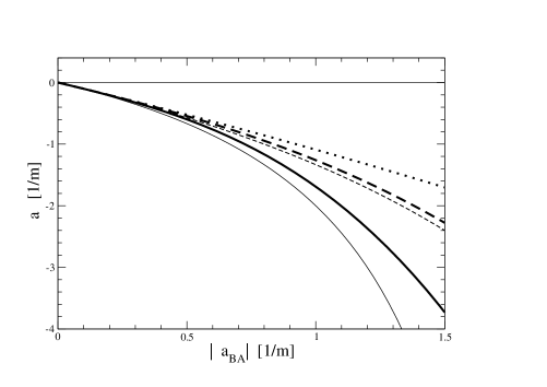
Figure 1: The scattering lengths, calculated by using Eq. (54), i.e. corresponding to solutions of the inhomogeneous BSE at zero-energy, vs $|a_{BA}|$ (Eq. (55)). Thick-solid line: $a$ for $\mu/m=1$. Thick-dashed line: $a$ for $\mu/m=0.5$. Thick-dotted line: $a$ for $\mu/m=0.15$. The non relativistic scattering lengths, represented by the corresponding thin lines, have been calculated by using Eq. (66). Notice that for $\mu/m=0.15$ the non relativistic calculation largely overlaps the relativistic one (thick-dotted line), and therefore it is indistinguishable.

In Fig. 2, the Nakanishi weight functions for (i) $\mu/m=0.15,~{}0.5,~{}1.0$, (ii) $\alpha=0.1,~{}2.5$, and (iii) $z=0$, but running $\gamma/m^{2}$, are shown. It should be pointed out that, for each value of $\mu/m$, the two values of the coupling constant $\alpha$ are representatives of a weak-interaction regime and a strong one. Moreover, since the Nakanishi weight functions obtained from Eq. (56) and Eq. (59) substantially coincide, only the calculations corresponding to Eq. (56) are shown. As mentioned at the beginning of this Section, the step-function behavior for small $\gamma$ has to be present, and the discontinuities are needed for obtaining the expected singularities in $\psi_{dist}$, like the one due to the global propagation. In Fig.2, the transition from the weak regime to the strong one increases the discontinuous behavior, that for large $\mu$ become more and more smooth. Finally, recalling that for a bound state and $\mu\to 0$, i.e. the Wick-Cutkosky model GW ; Cut , the Nakanishi weight function becomes proportional to $\delta(\gamma)$, it is instructive to see the onset of such a behavior in the upper part of Fig.2.

For $\gamma=0$ and $|z|\neq 1$, only the first part of the decomposition in Eq. (62), i.e. $g^{(+)}_{0Ld}(\gamma,z)\sim~{}\beta~{}\theta(\mu^{2}(1-|z|))$, is dominant, and therefore trivial.

In Fig. 3, the same quantities as in Fig. 2, but for $\gamma/m^{2}=0.1$ and running $z$, are also shown. As illustrated by the figure, the Nakanishi weight function acquaints a quite discontinuos behaviour, as $\mu/m$ increases.

Indeed, it is more profitable to present LF distributions, obtained from the distorted part of the zero-energy 3D scattering wave function. In analogy with the bound-state case (see Refs. FSV2 ; FSV3 ), one can construct transverse and longitudinal LF momentum distributions. In particular, one gets the following expression for $\psi^{(Ld)}_{dist}\left(z,\gamma;\kappa^{2}=z_{i}=0\right)$

$$\psi^{(Ld)}_{dist}\left(z,\gamma;\kappa^{2}=z_{i}=0\right)=$$

$$={(1-z^{2})\over 4}~{}\int_{0}^{\infty}d\gamma^{\prime}\frac{g^{(+)}_{0Ld}(\gamma^{\prime},z)}{[\gamma^{\prime}+\gamma+z^{2}m^{2}]^{2}}\,.$$ (67)

It should be noticed that inserting in Eq. (67) only the first part of the decomposition (62), one quickly reobtains the singular behavior due to the global propagation as shown in Eq. (12), viz

$$\psi^{(Ld)}_{dist}\left(z,\gamma;\kappa^{2}=z_{i}=0\right)\sim~{}\beta{(1-z^{2})\over 4}$$

$$\times~{}\left[{1\over\gamma+z^{2}m^{2}}-{1\over\mu^{2}(1-|z|)+\gamma+z^{2}m^{2}}\right]=\beta$$

$$\times~{}{(1-z^{2})\over 4}\left[{\mu^{2}(1-|z|)\over(\gamma+z^{2}m^{2})~{}[\mu^{2}(1-|z|)+\gamma+z^{2}m^{2}]}\right]\,.$$

(68)

Therefore, one has to expect singularities in the LF momentum distributions, that we would introduce in analogy with the ones for the bound states FSV2 . Let us emphasize, that only for the bound states they have a probabilistic interpretation. One could defines (i) the distorted transverse LF distribution

$${\cal P}_{dist}(\gamma)={1\over 2(2\pi)^{3}}~{}\int_{0}^{1}{d\xi\over 2~{}\xi(1-\xi)}~{}$$

$$\times\int_{0}^{2\pi}d\phi~{}[\psi^{(Ld)}_{dist}\left(z,\gamma;\kappa^{2}=z_{i}=0\right)]^{2}={1\over(16\pi)^{2}}$$

$$\times\int_{-1}^{1}dz~{}(1-z^{2})\left[\int_{0}^{\infty}d\gamma^{\prime}~{}{g^{(+)}_{0Ld}(\gamma^{\prime},z)\over[\gamma^{\prime}+\gamma+z^{2}m^{2}]^{2}}\right]^{2}\,,$$

(69)

and (ii) the longitudinal one, viz

$$\phi_{dist}(\xi)={1\over(2\pi)^{3}}~{}{1\over 2~{}\xi(1-\xi)}$$

$$\times~{}\int d{\bf k}_{\perp}~{}[\psi^{(Ld)}_{dist}\left(z,\gamma;\kappa^{2}=z_{i}=0\right)]^{2}=~{}2~{}{(1-z^{2})\over(16\pi)^{2}}$$

$$\times~{}\int_{0}^{\infty}d\gamma~{}\left[\int_{0}^{\infty}d\gamma^{\prime}~{}{g^{(+)}_{0Ld}(\gamma^{\prime},z)\over[\gamma^{\prime}+\gamma+z^{2}m^{2}]^{2}}\right]^{2}\,,$$

(70)

with the fraction of longitudinal momentum given by

$$\xi={1-z\over 2}=~{}{1\over p^{+}}~{}\left({p^{+}\over 2}+k^{+}\right)\,.$$ (71)

For the sake of presentation, it is useful to partially removing the singularities affecting the above distributions. Therefore, in Fig. 4, $\gamma^{2}~{}{\cal P}(\gamma)$ and $|1-2\xi|^{3/2}\phi(\xi)$ are shown. Figure 4 illustrates the overall behavior of the LF distributions by varying the coupling $\alpha$ and the mass of the exchanged scalar $\mu$, as in Figs. 2 and 3. It is worth noting the order-of-magnitude differences, when the coupling $\alpha$ is changed, but the typical features that one expects are still recognizable. A part the divergent behavior, already pointed out, that can be ascribed to the global propagation, the transverse distribution shows the ultraviolet tail produced by the dominance of a single exchanged scalar, exactly as in the case of the corresponding distribution for bound states (see Ref. FSV3 ). As to the longitudinal distributions, the expected peak at $\xi=1/2$ or $z=0$ is also seen.

The practical use of $\psi_{dist}$ is given by the evaluation of reactions that need a reliable treatment of the relativistic effects, i.e. when the coupling constant becomes larger and larger.

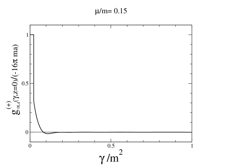
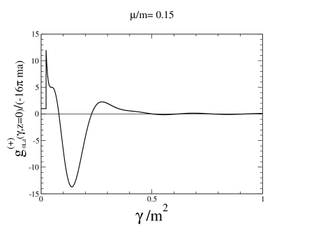
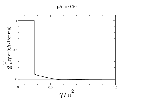
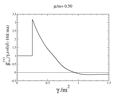
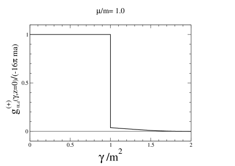
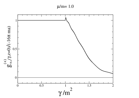
Figure 2: The Nakanishi weight function $g^{(+)}_{0Ld}(\gamma,z)$, in the zero-energy limit, vs $\gamma/m^{2}$, for $\mu/m=0.15,~{}0.5,~{}1.0$ and $z=0$, Left panels: weak-interaction regime with a chosen value $\alpha=0.1$. Right panels: strong-interaction regime with a chosen value $\alpha=2.5$.

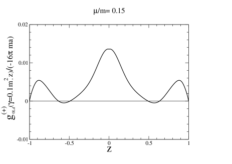
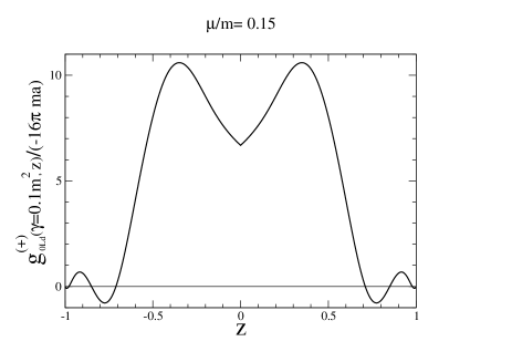
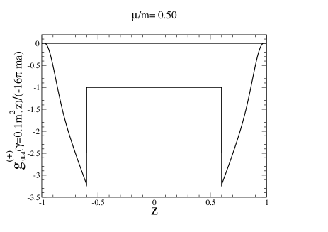
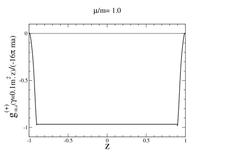
Figure 3: The same as in Fig. 2 but for running $z$, and $\gamma=0.1~{}m^{2}$.

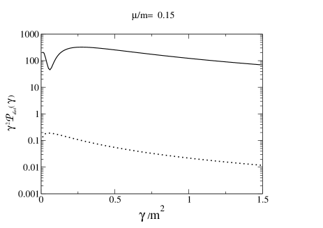
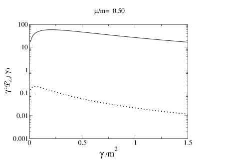
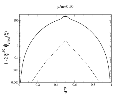
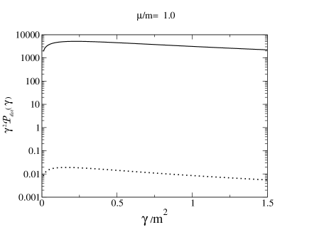
Figure 4: The LF distributions obtained from the distorted part of the 3D LF scattering wave function (see Eq. (67) for $\mu/m=0.15,~{}0.5,~{}1.0$ and zero-energy limit. Left panels: transverse LF-distribution $\gamma^{2}~{}{\cal P}(\gamma)$ vs the $\gamma/m^{2}$ (cf the transverse LF-distribution expression in Eq.(69)). Solid line: strong-interaction regime with $\alpha=2.5$; dotted line: weak-interaction regime with $\alpha=0.1$ Right panels: the same as in the left panel, but for $|1-2\xi|^{3/2}\phi(\xi)$, (cf the longitudinal LF-distribution in Eq. 70)

5 Conclusions

In the present paper, our approach FSV1 ; FSV2 ; FSV3 , based on the Nakanishi integral representation of the Bethe-Salpeter amplitude, is extended for the first time to the quantitative investigation of the zero-energy limit of the inhomogeneous Bethe-Salpeter Equation, in ladder approximation, for an interacting system composed by two massive scalars that exchange a massive scalar. This achievement represents a non trivial task, that has allowed us to gain a sound confidence in the Nakanishi Ansatz, as an effective and workable tool for obtaining actual solutions of the homogeneous and inhomogeneous BSE’s in Minkowski space. Indeed, the same approach that leads to a careful description of the bound states also yields a very accurate evaluation of the scattering length, as shown in Tables 1, 2 and 3 by the quantitative comparisons with the same observable evaluated within a totally different framework, based on the direct calculation of the contributions from the singularities of the inhomogeneous BSE carbonell6 ; carbonell7 .

As in the bound state case, we have performed the calculations by using the integral representation of the BS amplitude in terms of the Nakanishi weight function, Eq. (1), that explicitly shows the analytic dependence of the BS amplitude upon the invariant kinematical scalars of the scattering process, under scrutiny. Then, by applying the LF projection onto the null-plane to the inhomogeneous BSE in Minkowski space, Eq. (4) (without self-energy and vertex corrections), one is able to formally obtain the inhomogeneous integral equation for the Nakanishi weight function, that depends upon real variables. Its expression in ladder approximation is given by Eq. (18). Eventually, one can deduce another inhomogeneous integral equation for the Nakanishi weight function, Eq. (26), by assuming to be valid the uniqueness of the Nakanishi weight function, also in the non perturbative regime (recall that the theorem was demonstrated by Nakanishi nak71 in a perturbative framework, but taking into account the whole set of infinite diagrams contributing to a given $n$-leg amplitude).

The numerical comparisons for the scattering lengths, obtained by using our Eqs (56) and (59), and the corresponding quantities calculated in Ref. carbonell6 are shown in great detail in Tables 1, 2 and 3. It has to be emphasized that the high accuracy reached by our calculations is due to the new decomposition (62), suitable for obtaining the numerical solutions of the two inhomogeneous integral equations, involving the Nakanishi weight function. The comparison with the non relativistic scattering lengths (cf Fig. 1) has illustrated the potential impact of a proper treatment of the relativistic effects in the investigation of hadronic scattering states, even in the low-energy regime.

For the sake of completeness, the behavior of the Nakanishi weight functions, in the zero-energy limit, for weak- and strong interaction regimes have been shown in Figs. 2 and 3. Those figures illustrate the non smooth behavior of the Nakanishi weight functions for certain ranges of the variables, that is an inheritance of the singular behavior of the scattering states. Finally, we have defined LF momentum distributions, longitudinal and transverse ones, in analogy with the bound state case, (but without the probabilistic interpretation, entailed from the normalization of a bound state). Those distributions are shown in Fig. 4, for the sake of illustration and reference purpose. It should be noticed that the transverse LF distributions show the expected ultraviolet behavior, i.e. a power-like one, already found in the bound state case.

In conclusion, the Nakanishi Ansatz for the BS amplitude allows one to numerically solve in a very accurate way the inhomogeneous BSE, at least for the zero-energy limit. Such an outcome of our approach, together with the very nice results obtained for the bound-state case, strongly encourages to move to positive-energy scattering states, in order to evaluate the phase-shifts. If the phase-shifts evaluated within our approach (presented elsewhere FSV4 ) will agree with the ones in literaturecarbonell6 , then the reliability of the Nakanishi Ansatz as a starting guess for obtaining exact solutions of BSE’s in Minkowski space could make a substantial step forwards, confirming the great potentiality of this method, that can be applied to many other cases, changing dimensions Vito , statistics, kernels, etc.

Appendix A Boundary properties of the Nakanishi weight function $g^{(+)}(\gamma^{\prime},z^{\prime},z^{\prime\prime})$

This Appendix is devoted to the analysis of the relation between (i) the Nakanishi weight function $g^{(+)}(\gamma^{\prime},z^{\prime},z^{\prime\prime})$, that yields the integral representation of the distorted part of the 3D LF scattering wave function, and (ii) the weight function $\widetilde{\cal G}^{+}(\gamma^{\prime\prime},\zeta,\zeta^{\prime})$, that yields the integral representation of the half-off-shell T-matrix (cf Eq. (58) in Ref. FSV1 ). Notice that the dependence upon $\kappa^{2}$ and $z_{i}$ has been dropped for the sake of a light notation. This analysis allows one to obtain the conditions fulfilled by $g^{(+)}(\gamma^{\prime},z^{\prime},z^{\prime\prime})$ when $z^{\prime}=\pm 1$ and $z^{\prime\prime}=\pm 1$.

It is worth noting that while for $\widetilde{\cal G}^{+}(\gamma^{\prime\prime},\zeta,\zeta^{\prime})$ the constraint $\theta(1-|\zeta|-|\zeta^{\prime}|)$ holds, for the variables $z$ and $z^{\prime}$ an analogous relation does not exist.

The above mentioned relation between $g^{(+)}(\gamma^{\prime},z^{\prime},z^{\prime\prime})$ and $\widetilde{\cal G}^{+}(\gamma^{\prime\prime},\zeta,\zeta^{\prime})$ reads as follows (cf Eq. (63) in Ref. FSV1 , where a factor of two is missing, as well as in Eq. (60), but it was not relevant for the formal discussion, since it can be reabsorbed in $\widetilde{\cal G}^{+}$)

$$g^{(+)}(\gamma^{\prime},z^{\prime},z^{\prime\prime})=~{}i~{}2~{}\int_{0}^{1}d\alpha_{1}\int_{0}^{1}d\alpha_{2}~{}{1\over(1-\alpha_{1}-\alpha_{2})^{3}}$$

$$\times\theta(1-\alpha_{1}-\alpha_{2})~{}\theta(1-\alpha_{1}-\alpha_{2}-|z^{\prime}|-|z^{\prime\prime}-\alpha_{1}+\alpha_{2}|)$$

$$\times~{}\widetilde{\cal G}^{+}\left({\gamma^{\prime}\over(1-\alpha_{1}-\alpha_{2})},{z^{\prime}\over(1-\alpha_{1}-\alpha_{2})},{z^{\prime\prime}-\alpha_{1}+\alpha_{2}\over(1-\alpha_{1}-\alpha_{2})}\right)\,,$$

where

$$z^{\prime}=\zeta~{}(1-\alpha_{1}-\alpha_{2})$$

$$z^{\prime\prime}=\zeta^{\prime}~{}(1-\alpha_{1}-\alpha_{2})+\alpha_{1}-\alpha_{2}\,.$$ (73)

Notice that the constraints $\theta(1-\alpha_{1}-\alpha_{2})$ and $\theta(1-|\zeta|-|\zeta^{\prime}|)=\theta(1-\alpha_{1}-\alpha_{2}-|z^{\prime}|-|z^{\prime\prime}-\alpha_{1}+\alpha_{2}|)$ have been explicitly written, differently from Eq. (58) in Ref. FSV1 .

In what follows it will be shown that the above theta functions lead to a vanishing Nakanishi weight function at $|z^{\prime}|=1$ or $|z^{\prime\prime}|=1$.

Given the presence of $\theta(1-\alpha_{1}-\alpha_{2}-|z^{\prime}|-|z^{\prime\prime}-\alpha_{1}+\alpha_{2}|)$ and $0\leq\alpha_{i}\leq 1$, it is easily seen that for $|z^{\prime}|=1$ one has

$$g^{(+)}(\gamma^{\prime},z^{\prime}=\pm 1,z^{\prime\prime})=0$$

The same holds for $|z^{\prime\prime}|=1$. First of all, let us perform a change of variables, viz

$$\xi=1-(\alpha_{1}+\alpha_{2})~{},\quad\quad\quad\quad\Delta=\alpha_{1}-\alpha_{2}$$

$$\alpha_{1}={1-\xi+\Delta\over 2}~{},\quad\quad\quad\quad\alpha_{2}={1-\xi-\Delta\over 2}\,.$$ (74)

then Eq. (A) becomes

$$g^{(+)}(\gamma^{\prime},z^{\prime},z^{\prime\prime})=~{}i~{}2~{}{1\over 2}\int_{0}^{1}d\xi$$

$$\times\int_{-1}^{1}d\Delta~{}{\theta(1-\xi+\Delta)~{}\theta(1-\xi-\Delta)\over\xi^{3}}$$

$$\times~{}\widetilde{\cal G}^{+}\left({\gamma^{\prime}\over\xi},{z^{\prime}\over\xi},{z^{\prime\prime}-\Delta\over\xi}\right)\theta(\xi-|z^{\prime}|-|z^{\prime\prime}-\Delta|)\,.$$ (75)

For $z^{\prime\prime}=1$, one gets $z^{\prime\prime}-\Delta\geq 0$, since $\Delta\in[-1,1]$. Then

$$\theta(1-\xi-|\Delta|)~{}\theta(\xi-|z^{\prime}|-1$$

$$+\Delta)=\theta(1-\xi-|\Delta|)~{}\theta[\Delta-(1-\xi)-|z^{\prime}|]=0$$

since $\Delta\geq(1-\xi)+|z^{\prime}|\geq 0$ and $1-\xi\geq|\Delta|$. For $z^{\prime\prime}=-1$, one has $z^{\prime\prime}-\Delta\leq 0$, and then

$$\theta(1-\xi-|\Delta|)~{}\theta[\xi-|z^{\prime}|$$

$$-(1+\Delta)]=\theta(1-\xi-|\Delta|)~{}\theta[-(1-\xi)-|z^{\prime}|-\Delta]=0$$

since $-\Delta\geq(1-\xi)+|z^{\prime}|\geq 0$ and $1-\xi\geq|\Delta|$. Therefore, from the above results, one gets

$$g^{(+)}(\gamma^{\prime},z^{\prime},z^{\prime\prime}=\pm 1)=0$$

.

Appendix B The distorted part of the 3D LF scattering wave function

In this Appendix, it will be shown how the expected global free propagation of the constituents can be factorized out in the expression of $\psi^{(+)}_{dist}$, as in the non relativistic case. This result is relevant in two respects. On one side, it emphasizes the analogy with the non relativistic approach, and on the other side it allows one to understand the support of the Nakanishi weight function $g^{(+)}(\gamma^{\prime},z^{\prime},z;\gamma_{i},z_{i})$, when $\gamma^{\prime}$ runs.

In the CM frame ($\mathbf{p}_{\perp}=0$ and $p^{\pm}=M$), assuming without loss of generality a head-on scattering, i.e. $\gamma_{i}=0$, the 3D LF scattering wave function, is given by FSV1

$$\psi^{(+)}\left(z,\gamma;\kappa^{2},z_{i}\right)=p^{+}{(1-z^{2})\over 4}\int{dk^{-}\over 2\pi}~{}\Phi^{(+)}(k,p)=$$

$$=p^{+}{(1-z^{2})\over 4}~{}(2\pi)^{3}\delta^{(3)}(\tilde{k}-\tilde{k}_{i})+\psi_{dist}(z,\gamma;\kappa^{2},z_{i})\,,$$

where $\tilde{k}\equiv\{k^{+},{\bf k}_{\perp}\}$ and $\psi_{dist}$ is

$$\psi_{dist}(z,\gamma;\kappa^{2},z_{i})={(1-z^{2})\over 4}\int_{-1}^{1}dz^{\prime}\int_{-\infty}^{\infty}d\gamma^{\prime}$$

$$\frac{g^{(+)}(\gamma^{\prime},z^{\prime},z;\kappa^{2},z_{i})}{[\gamma^{\prime}+\gamma+z^{2}m^{2}+(1-z^{2})\kappa^{2}+{M^{2}\over 2}z~{}z^{\prime}z_{i}-i\epsilon]^{2}}\,,$$

By using the Nakanishi weight function for the half-off-shell T-matrix, one gets the following expression FSV1

$$\psi_{dist}(z,\gamma;\kappa^{2},z_{i})=$$

$$=p^{+}{(1-z^{2})\over 4}\int{dk^{-}\over 2\pi}~{}\langle k^{\mu}|G_{0}(p)T(p)|k^{\mu}_{i}\rangle=$$

$$=~{}p^{+}{(1-z^{2})\over 4}\int{dk^{-}\over 2\pi}~{}{i\over\left({p\over 2}+k\right)^{2}-m^{2}+i\epsilon}$$

$$\times{i\over\left({p\over 2}-k\right)^{2}-m^{2}+i\epsilon}\int_{-1}^{1}dz^{\prime}\int_{-1}^{1}d\zeta^{\prime}\int_{-\infty}^{\infty}d\gamma^{\prime}$$

$$\times~{}{\widetilde{\cal G}^{+}(\gamma^{\prime},z^{\prime},\zeta^{\prime};\kappa^{2},z_{i})~{}\theta(1-|z^{\prime}|-|\zeta^{\prime}|)\over k^{2}+{p^{2}\over 4}-m^{2}+\zeta^{\prime}p\cdot k+z^{\prime}2k\cdot k_{i}-\gamma^{\prime}+i\epsilon}\,.$$ (78)

Then, one can write

$$\psi_{dist}(z,\gamma;\kappa^{2},z_{i})=$$

$$=~{}-~{}p^{+}{(1-z^{2})\over 4}\int_{-1}^{1}dz^{\prime}\int_{-1}^{1}d\zeta^{\prime}\int_{-\infty}^{\infty}d\gamma^{\prime}$$

$$\times~{}\widetilde{\cal G}^{+}(\gamma^{\prime},z^{\prime},\zeta^{\prime};\kappa^{2},z_{i})~{}\theta(1-|z^{\prime}|-|\zeta^{\prime}|)\int{dk^{-}\over 2\pi}~{}$$

$$\times~{}{1\over(M/2+k^{+})~{}(M/2-k^{+})}~{}{1\over(k^{+}+\zeta^{\prime}{M\over 2}+z^{\prime}k^{+}_{i})}\times$$

$${1\over(\frac{p}{2}+k)^{-}-(\frac{p}{2}+k)^{-}_{on}+i\epsilon/(M/2+k^{+})}$$

$$\times~{}{1\over(\frac{p}{2}-k)^{-}-(\frac{p}{2}-k)^{-}_{on}+i\epsilon/(M/2-k^{+})}~{}\times$$

$${1\over k^{-}+{k^{+}(\zeta^{\prime}{M\over 2}+z^{\prime}k^{-}_{i})-\gamma-\gamma^{\prime}-\kappa^{2}+i\epsilon\over(k^{+}+\zeta^{\prime}{M\over 2}+z^{\prime}k^{+}_{i})}}\,,$$ (79)

where

$$(\frac{p}{2}+k)^{-}_{on}={2(m^{2}+\gamma)\over M(1-z)}$$

$$(\frac{p}{2}-k)^{-}_{on}={2(m^{2}+\gamma)\over M(1+z)}\,.$$ (80)

with $k^{+}=-zM/2$. Since $k^{+}_{i}=-k^{-}_{i}=-z_{i}M/2$, one gets

$$\psi_{dist}(z,\gamma;\kappa^{2},z_{i})=~{}-~{}{2\over M^{2}}\int_{-1}^{1}dz^{\prime}\int_{-1}^{1}d\zeta^{\prime}\int_{-\infty}^{\infty}d\gamma^{\prime}$$

$$\times~{}\widetilde{\cal G}^{+}(\gamma^{\prime},z^{\prime},\zeta^{\prime};\kappa^{2},z_{i})~{}{\theta(1-|z^{\prime}|-|\zeta^{\prime}|)\over(\zeta^{\prime}-z-z^{\prime}z_{i})}$$

$$\times\int{dk^{-}\over 2\pi}~{}{1\over\frac{M}{2}+k^{-}-(\frac{p}{2}+k)^{-}_{on}+i2\epsilon/[M/(1-z)]}~{}~{}$$

$$\times{1\over\frac{M}{2}-k^{-}-(\frac{p}{2}-k)^{-}_{on}+i2\epsilon/[M(1+z)]}~{}\times$$

$${1\over[k^{-}-k_{Na}^{-}+i2\epsilon/[M(\zeta^{\prime}-z-z^{\prime}z_{i})]}\,,$$ (81)

with

$$k_{Na}^{-}={2\over M(\zeta^{\prime}-z-z^{\prime}z_{i})}$$

$$\times~{}\left[{M^{2}\over 4}z(\zeta^{\prime}+z^{\prime}z_{i})+\gamma+\gamma^{\prime}+\kappa^{2}\right]\,.$$ (82)

One has the following poles (recall that $1>z>-1$)

$$k_{L}=(\frac{p}{2}+k)^{-}_{on}-{M\over 2}-i\epsilon$$

$$k_{U}=-(\frac{p}{2}-k)^{-}_{on}+{M\over 2}+i\epsilon$$

$$k_{LU}=k_{Na}^{-}-i{2\epsilon\over M(\zeta^{\prime}-z-z^{\prime}z_{i})}\,.$$ (83)

In order to evaluate the analytic integration on $k^{-}$, one can consider the following two cases.

If $\zeta^{\prime}>z+z^{\prime}z_{i}$, one can close the integration contour into the upper plane, taking the residue at $k_{U}$, i.e.

$$\int_{-\infty}^{\infty}{dk^{-}\over 2\pi}~{}{1\over\left[k^{-}-k_{L}\right]}~{}{1\over\left[-k^{-}+k_{U}\right]}~{}{1\over\left[k^{-}-k_{LU}\right]}=$$

$$=-i{1\over\left[M-(\frac{p}{2}-k)^{-}_{on}-(\frac{p}{2}+k)^{-}_{on}+i\epsilon\right]}$$

$$\times~{}{1\over\left[{M\over 2}-(\frac{p}{2}-k)^{-}_{on}-k_{Na}^{-}+i\epsilon\right]}=$$

$$=-i~{}{M^{2}\over 8}~{}(\zeta^{\prime}-z-z^{\prime}z_{i})$$

$$\times~{}{(1-z^{2})\over\left[\kappa^{2}(1-z^{2})+m^{2}z^{2}+\gamma-i\epsilon\right]}~{}{(1+z)\over(1+\zeta^{\prime}-z^{\prime}z_{i})}~{}\times$$

$${1\over\kappa^{2}(1-z^{2})+m^{2}z^{2}+\gamma+{(1+z)\left({M^{2}\over 2}zz^{\prime}z_{i}+\gamma^{\prime}\right)\over(1+\zeta^{\prime}-z^{\prime}z_{i})}-i\epsilon}\,.$$

If $z+z^{\prime}z_{i}>\zeta^{\prime}$, one can close the integration contour into the lower plane, taking the residue at $k_{L}$, i.e.

$$\int_{-\infty}^{\infty}{dk^{-}\over 2\pi}~{}{1\over\left[k^{-}-k_{L}\right]}~{}{1\over\left[-k^{-}+k_{U}\right]}~{}{1\over\left[k^{-}-k_{LU}\right]}=$$

$$=~{}-i{M^{2}\over 8}~{}(\zeta^{\prime}-z-z^{\prime}z_{i})$$

$$\times~{}{(1-z)\over(1-\zeta^{\prime}+z^{\prime}z_{i})}~{}{(1-z^{2})\over\left[\kappa^{2}(1-z^{2})+m^{2}z^{2}+\gamma-i\epsilon\right]}~{}$$

$$\times{1\over\kappa^{2}(1-z^{2})+m^{2}z^{2}+\gamma+{(1-z)\left({M^{2}\over 2}zz^{\prime}z_{i}+\gamma^{\prime}\right)\over(1-\zeta^{\prime}+z^{\prime}z_{i})}~{}-i\epsilon}\,,$$

where $(\zeta^{\prime}-z-z^{\prime}z_{i})\epsilon\to-\epsilon$, since $(\zeta^{\prime}-z-z^{\prime}z_{i})<0$.

Collecting all the above results, one gets the following expression for $\psi_{dist}$

$$\psi_{dist}(z,\gamma;\kappa^{2},z_{i})=$$

$$=~{}i~{}{(1-z^{2})\over 4}~{}{1\over\left[\kappa^{2}(1-z^{2})+m^{2}z^{2}+\gamma-i\epsilon\right]}$$

$$\int_{-1}^{1}dz^{\prime}\int_{-1}^{1}d\zeta^{\prime}\int_{-\infty}^{\infty}d\gamma^{\prime}~{}\widetilde{\cal G}^{+}(\gamma^{\prime},z^{\prime},\zeta^{\prime};\kappa^{2},z_{i})~{}\times$$

$$\Bigl{[}{(1+z)\over(1+\zeta^{\prime}-z^{\prime}z_{i})}$$

$$\times~{}{\theta(\zeta^{\prime}-z-z^{\prime}z_{i})~{}\theta(1-|z^{\prime}|-|\zeta^{\prime}|)\over\kappa^{2}(1-z^{2})+m^{2}z^{2}+\gamma+{(1+z)\left({M^{2}\over 2}zz^{\prime}z_{i}+\gamma^{\prime}\right)\over(1+\zeta^{\prime}-z^{\prime}z_{i})}-i\epsilon}$$

$$+{(1-z)\over(1-\zeta^{\prime}+z^{\prime}z_{i})}$$

$$\times~{}{\theta(z+z_{i}z^{\prime}-\zeta^{\prime})~{}\theta(1-|z^{\prime}|-|\zeta^{\prime}|)\over\kappa^{2}(1-z^{2})+m^{2}z^{2}+\gamma+{(1-z)\left({M^{2}\over 2}zz^{\prime}z_{i}+\gamma^{\prime}\right)\over(1-\zeta^{\prime}+z^{\prime}z_{i})}~{}-i\epsilon}\Bigr{]}\,$$

. (86)

One can reobtain the expression in Eq. (B) by applying the Feynman trick to Eq. (86). For instance, one has

$${\theta(\zeta^{\prime}-z-z_{i}z^{\prime})\over\left[\kappa^{2}(1-z^{2})+m^{2}z^{2}+\gamma-i\epsilon\right]}$$

$$\times~{}{1\over\kappa^{2}(1-z^{2})+m^{2}z^{2}+\gamma+{(1+z)\left({M^{2}\over 2}zz^{\prime}z_{i}+\gamma^{\prime}\right)\over(1+\zeta^{\prime}-z^{\prime}z_{i})}-i\epsilon}=$$

$$=~{}\theta(\zeta^{\prime}-z-z_{i}z^{\prime})\int_{0}^{1}d\xi~{}\times$$

$${1\over\left[\gamma+m^{2}z^{2}+\kappa^{2}(1-z^{2})+\xi{(1+z)\left({M^{2}\over 2}zz^{\prime}z_{i}+\gamma^{\prime}\right)\over(1+\zeta^{\prime}-z^{\prime}z_{i})}-i\epsilon\right]^{2}}$$

$$={(1+\zeta^{\prime}-z^{\prime}z_{i})\over(1+z)}\int_{0}^{1}d\alpha~{}\theta\left[{(1+z)\over(1+\zeta^{\prime}-z^{\prime}z_{i})}-\alpha\right]~{}\times$$

$${\theta(\zeta^{\prime}-z-z_{i}z^{\prime})\over\left[\gamma+m^{2}z^{2}+\kappa^{2}(1-z^{2})+\alpha~{}\left({M^{2}\over 2}zz^{\prime}z_{i}+\gamma^{\prime}\right)-i\epsilon\right]^{2}}\,,$$

with

$$1\geq{(1+z)\over(1+\zeta^{\prime}-z^{\prime}z_{i})}={(1+z)\over[1+z+(\zeta^{\prime}-z-z^{\prime}z_{i})]}$$

since $\theta(\zeta^{\prime}-z-z_{i}z^{\prime})$. Inserting the above expression, together with the one containing $\theta(z+z_{i}z^{\prime}-\zeta^{\prime})$, in Eq. (86), one gets the following expression for the distorted term

$$\psi_{dist}(z,\gamma;z_{i},\kappa^{2})=$$

$$=~{}i~{}{(1-z^{2})\over 4}~{}\int_{-1}^{1}d\zeta^{\prime\prime}\int_{-1}^{1}d\zeta^{\prime}\int_{-\infty}^{\infty}d\gamma^{\prime\prime}~{}\int_{0}^{1}{d\alpha\over\alpha^{2}}$$

$$\times~{}\theta(\alpha-|\zeta^{\prime\prime}|)~{}\theta(1-|{\zeta^{\prime\prime}\over\alpha}|-|\zeta^{\prime}|)$$

$$\times~{}{\widetilde{\cal G}^{+}({\gamma^{\prime\prime}\over\alpha},{\zeta^{\prime\prime}\over\alpha},\zeta^{\prime})\over\left[\gamma+m^{2}z^{2}+\kappa^{2}(1-z^{2})+\gamma^{\prime\prime}+{M^{2}\over 2}z\zeta^{\prime\prime}z_{i}-i\epsilon\right]^{2}}$$

$$\left\{\theta\left[(1+z+\zeta^{\prime\prime}z_{i})-\alpha(1+\zeta^{\prime})\right]~{}\theta[\alpha(\zeta^{\prime}-z)-z_{i}\zeta^{\prime\prime}]+\right.$$

$$\left.\theta\left[(1-z-\zeta^{\prime\prime}z_{i})-\alpha(1-\zeta^{\prime}))\right]~{}\theta[-\alpha(\zeta^{\prime}-z)+z_{i}\zeta^{\prime\prime}]\right\}$$

$$=~{}i~{}{(1-z^{2})\over 4}~{}\int_{-1}^{1}d\zeta^{\prime\prime}\int_{-\infty}^{\infty}d\gamma^{\prime\prime}~{}\int_{0}^{1}{d\alpha\over\alpha^{3}}~{}\int_{-1}^{1}dy$$

$$\times\theta(\alpha-|y|)\theta(\alpha-|\zeta^{\prime\prime}|)~{}\theta(\alpha-|\zeta^{\prime\prime}|-|y|)$$

$$\times~{}{\widetilde{\cal G}^{+}({\gamma^{\prime\prime}\over\alpha},{\zeta^{\prime\prime}\over\alpha},{y\over\alpha})\over\left[\gamma+m^{2}z^{2}+\kappa^{2}(1-z^{2})+\gamma^{\prime\prime}+{M^{2}\over 2}z\zeta^{\prime\prime}z_{i}-i\epsilon\right]^{2}}$$

$$\left\{\theta\left(1+z+\zeta^{\prime\prime}z_{i}-\alpha-y\right)~{}\theta(y-\alpha z-z_{i}\zeta^{\prime\prime})+\right.$$

$$\left.\theta\left(1-z-\zeta^{\prime\prime}z_{i}-\alpha+y\right]~{}\theta[-y+\alpha z+z_{i}\zeta^{\prime\prime})\right\}\,,$$ (88)

where $\gamma^{\prime\prime}=\alpha~{}\gamma^{\prime}$ and $\zeta^{\prime\prime}=\alpha~{}z^{\prime}$.

The theta functions between curly brackets single out the following integration regions

• $1-\alpha+z+\zeta^{\prime\prime}z_{i}\geq y\geq\alpha z+z_{i}\zeta^{\prime\prime}$

• $\alpha z+z_{i}\zeta^{\prime\prime}\geq y\geq-(1-\alpha)+z+\zeta^{\prime\prime}z_{i}$

The above intervals lead to the following constraint

$$1-\alpha\geq y-z-\zeta^{\prime\prime}z_{i}\geq-(1-\alpha)$$

namely $\theta(1-\alpha-|y-z-\zeta^{\prime\prime}z_{i}|)$ . Then one gets

$$\psi_{dist}(z,\gamma;z_{i},\kappa^{2})=~{}i~{}{(1-z^{2})\over 4}~{}\int_{-1}^{1}d\zeta^{\prime\prime}\int_{-\infty}^{\infty}d\gamma^{\prime\prime}$$

$$\times~{}\int_{0}^{1}{d\alpha\over\alpha^{3}}~{}\int_{-1}^{1}dy~{}\widetilde{\cal G}^{+}({\gamma^{\prime\prime}\over\alpha},{\zeta^{\prime\prime}\over\alpha},{y\over\alpha})$$

$$\times~{}{\theta(\alpha-|\zeta^{\prime\prime}|-|y|)~{}\theta(1-\alpha-|y-z-\zeta^{\prime\prime}z_{i}|)\over\left[\gamma+m^{2}z^{2}+\kappa^{2}(1-z^{2})+\gamma^{\prime\prime}+{M^{2}\over 2}z\zeta^{\prime\prime}z_{i}-i\epsilon\right]^{2}}\,.$$

The above expression of $\psi_{dist}$ allows one to write the following relation between the Nakanishi weight function $g^{+}(\gamma^{\prime},z^{\prime},z;\kappa^{2},z_{i})$, that appears in Eq. (B), and $\widetilde{\cal G}^{+}$, namely the Nakanishi weight function involved in the description the half-off-shell T-matrix,

$$g^{+}(\gamma^{\prime},z^{\prime},z;\kappa^{2},z_{i})=$$

$$=i\int_{0}^{1}{d\alpha\over\alpha^{3}}~{}\int_{-1}^{1}dy~{}\widetilde{\cal G}^{+}({\gamma^{\prime}\over\alpha},{z^{\prime}\over\alpha},{y\over\alpha};\kappa^{2},z_{i})$$

$$\times~{}\theta(\alpha-|z^{\prime}|-|y|)\theta(1-\alpha-|y-z-z^{\prime}z_{i}|)\,.$$ (90)

Notice that Eq. (90) can be transformed into Eq. (A) by applying a suitable change of variables.

Appendix C Zero-energy limit

The zero-energy limit of the relevant integral equations fulfilled by the Nakanishi weight function amounts to consider the case $\kappa^{2}=0$, namely $M^{2}=4m^{2}$. This entails $\gamma_{i}=z_{i}=0$ through $M^{2}=4(m^{2}+\gamma_{i})/(1-z^{2}_{i})$. In this Appendix, the integral equations obtained both without applying the uniqueness theorem nak71 and by exploiting it, are obtained following a simpler procedure than the one adopted in Ref. FSV1 (notice that a mistyping present in Eq. (103) of FSV1 has been fixed in this Appendix, as explained in what follows).

The Nakanishi integral equation, involving $\psi_{dist}$, for $\kappa^{2}\leq 0$ (see FSV1 ) is given by

$$\int_{-1}^{1}dz^{\prime}\int_{-\infty}^{\infty}d\gamma^{\prime\prime}~{}g^{(+)}_{(Ld)}(\gamma^{\prime\prime},z^{\prime},z;\gamma_{i},z_{i})$$

$$\times~{}\frac{1}{[\gamma+\gamma^{\prime\prime}+z^{2}m^{2}+(1-z^{2})\kappa^{2}+z^{\prime}{M^{2}\over 2}zz_{i}-i\epsilon]^{2}}=$$

$$=g^{2}~{}\int_{-1}^{1}dz^{\prime}~{}\int^{\infty}_{-\infty}~{}d\gamma^{\prime\prime}~{}\theta(-z^{\prime})~{}\delta(\gamma^{\prime\prime}-\gamma_{a}(z^{\prime}))$$

$$\times~{}{1\over\left[\gamma+\gamma^{\prime\prime}+(1-z^{2})\kappa^{2}+z^{2}m^{2}+z^{\prime}{M^{2}\over 2}zz_{i}-i\epsilon\right]^{2}}$$

$$\Bigl{\{}\theta(z-z_{i})~{}\theta\left[1-z+z^{\prime}(1-z_{i})\right]$$

$$+\theta(z_{i}-z)~{}\theta\left[1+z+z^{\prime}(1+z_{i})\right]\Bigr{\}}$$

$$-{g^{2}\over 2(4\pi)^{2}}~{}\int^{\infty}_{-\infty}d\gamma^{\prime\prime}\int^{1}_{-1}dz^{\prime}$$

$$\times{1\over\left[\gamma+\gamma^{\prime\prime}+z^{2}m^{2}+\kappa^{2}(1-z^{2})+z^{\prime}{M^{2}\over 2}zz_{i}-i\epsilon\right]^{2}}$$

$$\int_{-\infty}^{\infty}d\gamma^{\prime}\int_{-1}^{1}d\zeta\int_{-1}^{1}d\zeta^{\prime}~{}g^{(+)}_{(Ld)}(\gamma^{\prime},\zeta,\zeta^{\prime};\kappa^{2},z_{i})$$

$$\times\Bigl{[}{(1+z)\over(1+\zeta^{\prime}-z_{i}\zeta)}$$

$$\times~{}\theta(\zeta^{\prime}-z-z_{i}\zeta)~{}h^{\prime}(\gamma^{\prime\prime},z^{\prime},z,z_{i};\gamma^{\prime},\zeta,\zeta^{\prime},\mu^{2})$$

$$+{(1-z)\over(1-\zeta^{\prime}+z_{i}\zeta)}$$

$$\times~{}\theta(z-\zeta^{\prime}+z_{i}\zeta)~{}h^{\prime}(\gamma^{\prime\prime},z^{\prime},-z,-z_{i};\gamma^{\prime},\zeta,-\zeta^{\prime},\mu^{2})\Bigr{]}~{},$$

(91)

with

$$h^{\prime}(\gamma^{\prime\prime},z^{\prime},z,z_{i};\gamma^{\prime},\zeta,\zeta^{\prime},\mu^{2})=~{}{(1+z)\over(1+\zeta^{\prime}-z_{i}\zeta)}~{}\times$$

$$\left\{{\partial\over\partial\lambda}\int^{\infty}_{0}{dy}~{}\int_{0}^{1}d\xi~{}\delta\left[z^{\prime}-\xi Z(z,\zeta,\zeta^{\prime};z_{i})\right]~{}\times\right.$$

$$\left.\delta\left[{\cal F}(\lambda,y,\xi;\gamma^{\prime\prime},z,\zeta,\zeta^{\prime},\gamma^{\prime};z_{i},\kappa^{2},\mu^{2})\right]\right\}_{\lambda=0}\,.$$ (92)

where

$${\cal F}(\lambda,y,\xi;\gamma^{\prime\prime},z,\zeta,\zeta^{\prime},\gamma^{\prime};z_{i},\kappa^{2},\mu^{2})=$$

$$=\gamma^{\prime\prime}-\xi~{}{(1+z)\over(1+\zeta^{\prime}-z_{i}\zeta)}$$

$$\times~{}\left({y^{2}{\cal A}(\zeta,\zeta^{\prime},\gamma^{\prime},\kappa^{2})+y(\mu^{2}+\gamma^{\prime})+\mu^{2}\over y}\right)-\xi\lambda$$ (93)

For $\kappa^{2}=0$, it follows that $\gamma_{i}=z_{i}=0$ since

$$\kappa^{2}=m^{2}-{M^{2}\over 4}=\left({p\over 2}\pm k_{i}\right)^{2}-{M^{2}\over 4}=-\gamma_{i}-z^{2}_{i}{M^{2}\over 4}=0$$

Then, taking into account that $g^{(+)}_{(Ld)}(\gamma,z^{\prime},z;\kappa^{2}=0)$ has support only for positive $\gamma$, one can write (cf Eq. (91) and subsec. 2.2)

$$\int_{-1}^{1}dz^{\prime}\int_{0}^{\infty}d\gamma^{\prime\prime}~{}~{}\frac{g^{(+)}_{(Ld)}(\gamma^{\prime\prime},z^{\prime},z;\kappa^{2}=0)}{[\gamma+\gamma^{\prime\prime}+z^{2}m^{2}-i\epsilon]^{2}}=$$

$$=g^{2}~{}\int^{\infty}_{0}~{}d\gamma^{\prime\prime}~{}\int_{-1}^{1}dz^{\prime}~{}{\theta(-z^{\prime})~{}\delta(\gamma^{\prime\prime}+z^{\prime}\mu^{2})\over\left[\gamma+\gamma^{\prime\prime}+z^{2}m^{2}-i\epsilon\right]^{2}}$$

$$\times~{}\Bigl{[}\theta(z)~{}\theta\left(1-z+z^{\prime}\right)+\theta(-z)~{}\theta\left(1+z+z^{\prime}\right)\Bigr{]}$$

$$-{g^{2}\over 2(4\pi)^{2}}~{}\int_{0}^{\infty}d\gamma^{\prime}\int_{-1}^{1}d\zeta$$

$$\times\int_{-1}^{1}d\zeta^{\prime}~{}g^{(+)}_{(Ld)}(\gamma^{\prime},\zeta,\zeta^{\prime};\kappa^{2}=0)$$

$$\times\int^{\infty}_{-\infty}d\gamma^{\prime\prime}~{}{1\over\left[\gamma+\gamma^{\prime\prime}+z^{2}m^{2}-i\epsilon\right]^{2}}\int^{1}_{-1}dz^{\prime}$$

$$\times~{}\Bigl{[}{(1+z)\over(1+\zeta^{\prime})}~{}\theta(\zeta^{\prime}-z)~{}{\cal Z}^{\prime}(\gamma^{\prime\prime},z^{\prime},z;\gamma^{\prime},\zeta^{\prime},\mu^{2})$$

$$+{(1-z)\over(1-\zeta^{\prime})}~{}\theta(z-\zeta^{\prime})~{}{\cal Z}^{\prime}(\gamma^{\prime\prime},z^{\prime},-z;\gamma^{\prime},-\zeta^{\prime},\mu^{2})\Bigr{]}\,,$$

(94)

where the kernel ${\cal Z}^{\prime}$ is given by

$${\cal Z}^{\prime}(\gamma^{\prime\prime},z^{\prime},z;\gamma^{\prime},\zeta^{\prime},\mu^{2})={(1+z)\over(1+\zeta^{\prime})}~{}\times$$

$$\Bigl{\{}{\partial\over\partial\lambda}\int_{0}^{\infty}{dy}~{}\int_{0}^{1}d\xi\,\delta\left[\gamma^{\prime\prime}-\xi\Gamma_{0}(y,z,\zeta^{\prime},\gamma^{\prime})-\xi\lambda\right]$$

$$\times\delta\left[z^{\prime}-\xi{(1+z)\over(1+\zeta^{\prime})}~{}\zeta\right]\Bigr{\}}_{\lambda=0}$$ (95)

with

$$\Gamma_{0}(y,z,\zeta^{\prime},\gamma^{\prime})={(1+z)\over(1+\zeta^{\prime})}~{}{1\over y}$$

$$\times\left\{y^{2}~{}{\cal A}_{0}(\zeta^{\prime},\gamma^{\prime})+y(\mu^{2}+\gamma^{\prime})+\mu^{2}\right\}$$ (96)

and

$${\cal A}_{0}(\zeta^{\prime},\gamma^{\prime})={\zeta^{\prime}}^{2}\frac{M^{2}}{4}+\gamma^{\prime}=~{}{\zeta^{\prime}}^{2}m^{2}+\gamma^{\prime}~{}\geq~{}0\,,$$ (97)

Notice that $\gamma^{\prime}$ is positive and therefore also $\Gamma_{0}$ has to be positive. Finally, $\gamma^{\prime\prime}$ in Eq. (95) has to be positive for getting a non vanishing ${\cal Z}^{\prime}(\gamma^{\prime\prime},z^{\prime},z;\gamma^{\prime},\zeta^{\prime},\mu^{2})$.

Performing (i) the integration on $z^{\prime}$ in both sides of Eq. (94) (recall that $1>|\xi\zeta(1\pm z)/(1\pm\zeta^{\prime})|$) and (ii) the integration on $\zeta$ in the rhs, one gets

$$\int_{0}^{\infty}d\gamma^{\prime\prime}\frac{g^{(+)}_{0Ld}(\gamma^{\prime\prime},z)}{[\gamma+\gamma^{\prime\prime}+z^{2}m^{2}-i\epsilon]^{2}}=$$

$$={g^{2}\over\mu^{2}}~{}\int^{\infty}_{-\infty}~{}d\gamma^{\prime\prime}~{}{\theta(\gamma^{\prime\prime})\over\left[\gamma+\gamma^{\prime\prime}+z^{2}m^{2}-i\epsilon\right]^{2}}$$

$$\times~{}\Bigl{\{}\theta(z)~{}\theta\left[1-z-\gamma^{\prime\prime}/\mu^{2}\right]$$

$$+\theta(-z)~{}\theta\left[1+z-\gamma^{\prime\prime}/\mu^{2}\right]\Bigr{\}}+$$

$$-{g^{2}\over 2(4\pi)^{2}}~{}\int_{0}^{\infty}d\gamma^{\prime}\int_{-1}^{1}d\zeta^{\prime}~{}g^{(+)}_{0Ld}(\gamma^{\prime},\zeta^{\prime})$$

$$\times~{}\int^{\infty}_{-\infty}d\gamma^{\prime\prime}~{}\theta(\gamma^{\prime\prime})~{}~{}{1\over\left[\gamma+\gamma^{\prime\prime}+z^{2}m^{2}-i\epsilon\right]^{2}}\times$$

$$\Bigl{[}{(1+z)\over(1+\zeta^{\prime})}~{}\theta(\zeta^{\prime}-z)~{}{h}_{0}^{\prime}(\gamma^{\prime\prime},z;\gamma^{\prime},\zeta^{\prime},\mu^{2})$$

$$+{(1-z)\over(1-\zeta^{\prime})}~{}\theta(z-\zeta^{\prime})~{}{h}_{0}^{\prime}(\gamma^{\prime\prime},-z;\gamma^{\prime},-\zeta^{\prime},\mu^{2})\Bigr{]}\,,$$ (98)

where

1. $$g^{(+)}_{0Ld}(\gamma^{\prime\prime},z)=\int_{-1}^{1}dz^{\prime}g^{(+)}_{(Ld)}(\gamma^{\prime\prime},z^{\prime},z;\kappa^{2}=0)\,.$$ (99)

2. $$\int_{-1}^{1}dz^{\prime}~{}\theta(-z^{\prime})~{}\delta(\gamma^{\prime\prime}+z^{\prime}\mu^{2})=$$

   $$={1\over\mu^{2}}\theta(\gamma^{\prime\prime})\theta(\mu^{2}-\gamma^{\prime\prime})\,.$$ (100)

3. $${h}_{0}^{\prime}(\gamma^{\prime\prime},z;\gamma^{\prime},\zeta^{\prime},\mu^{2})={(1+z)\over(1+\zeta^{\prime})}~{}\left.{\partial\over\partial\lambda}\int_{0}^{\infty}{dy}\right.$$

   $$\left.~{}\int_{0}^{1}d\xi\,\delta\left[\gamma^{\prime\prime}-\xi\Gamma_{0}(y,z,\zeta^{\prime},\gamma^{\prime})-\xi\lambda\right]\,\right|_{\lambda=0}\,.$$

From Ref. FSV2 , one recognizes that ${h}_{0}^{\prime}(\gamma^{\prime\prime},z;\gamma^{\prime},\zeta^{\prime},\mu^{2})$ is the suitable kernel for a bound state with zero energy. Therefore one can write

$$h^{\prime}_{0}(\gamma^{\prime\prime},z;\gamma^{\prime},\zeta^{\prime},\mu^{2})=$$

$$=\theta\left[-~{}{\cal B}_{0}(z,\zeta^{\prime},\gamma^{\prime},\gamma^{\prime\prime},\mu^{2})-2\mu\sqrt{{\zeta^{\prime}}^{2}\frac{M^{2}}{4}+\gamma^{\prime}}\right]$$

$$\times\Bigl{[}-{{\cal B}_{0}(z,\zeta^{\prime},\gamma^{\prime},\gamma^{\prime\prime},\mu^{2})\over{\cal A}_{0}(\zeta^{\prime},\gamma^{\prime})~{}\Delta_{0}(z,\zeta^{\prime},\gamma^{\prime},\gamma^{\prime\prime},\mu^{2})}~{}{1\over\gamma^{\prime\prime}}+{(1+\zeta^{\prime})\over(1+z)}$$

$$\times~{}\int_{y_{-}}^{y_{+}}{dy}~{}{y^{2}\over\left[{y}^{2}{\cal A}_{0}(\zeta^{\prime},\gamma^{\prime})+y(\mu^{2}+\gamma^{\prime})+\mu^{2}\right]^{2}}\Bigr{]}$$

$$-{(1+\zeta^{\prime})\over(1+z)}~{}\int_{0}^{\infty}{dy}~{}{y^{2}\over\left[{y}^{2}{\cal A}_{0}(\zeta^{\prime},\gamma^{\prime})+y(\mu^{2}+\gamma^{\prime})+\mu^{2}\right]^{2}}\,,$$

(102)

with (see also Eq. (97))

$${\cal B}_{0}(z,\zeta^{\prime},\gamma^{\prime},\gamma^{\prime\prime},\mu^{2})=\mu^{2}+\gamma^{\prime}-\gamma^{\prime\prime}{(1+\zeta^{\prime})\over(1+z)}~{}\leq 0~{}~{},$$

$$\Delta^{2}_{0}(z,\zeta^{\prime},\gamma^{\prime},\gamma^{\prime\prime},\mu^{2})=$$

$$={\cal B}_{0}^{2}(z,\zeta^{\prime},\gamma^{\prime},\gamma^{\prime\prime},\mu^{2})-4\mu^{2}~{}{\cal A}_{0}(\zeta^{\prime},\gamma^{\prime})~{}\geq~{}0~{}~{},$$

$$y_{\pm}={1\over 2{\cal A}_{0}(\zeta^{\prime},\gamma^{\prime})}$$

$$\times~{}\left[-{\cal B}_{0}(z,\zeta^{\prime},\gamma^{\prime},\gamma^{\prime\prime},\mu^{2})\pm\Delta_{0}(z,\zeta^{\prime},\gamma^{\prime},\gamma^{\prime\prime},\mu^{2})\right]\,.$$ (103)

Notice that in the inhomogeneous term in Eq. (98) the factor $\theta(\mu^{2}-\gamma^{\prime\prime})$ has been dropped, given the presence of the step functions $\theta\left[1\pm z-\gamma^{\prime\prime}/\mu^{2}\right]$. In Eq. (103) of Ref. FSV1 the step function $\theta(\mu^{2}-\gamma^{\prime\prime})$ has been accidentally overlooked.

In conclusion, by applying the Nakanishi theorem on the uniqueness of the weight function nak71 , one has the following integral equation

$$g^{(+)}_{0Ld}(\gamma,z)={g^{2}\over\mu^{2}}~{}\theta(\gamma)~{}\theta\left[\mu^{2}(1-|z|)-\gamma\right]$$

$$-{g^{2}\over 2(4\pi)^{2}}~{}\theta(\gamma)~{}\int_{0}^{\infty}d\gamma^{\prime}\int_{-1}^{1}dz^{\prime}~{}g^{(+)}_{0Ld}(\gamma^{\prime},z^{\prime})~{}\times$$

$$\Bigl{[}{(1+z)\over(1+z^{\prime})}~{}\theta(z^{\prime}-z)~{}{h}_{0}^{\prime}(\gamma,z;\gamma^{\prime},z^{\prime},\mu^{2})$$

$$+{(1-z)\over(1-z^{\prime})}~{}\theta(z-z^{\prime})~{}{h}_{0}^{\prime}(\gamma,-z;\gamma^{\prime},-z^{\prime},\mu^{2})\Bigr{]}\,.$$ (104)

Appendix D An effective decomposition of $g^{(+)}_{0Ld}(\gamma,z)$

In this Appendix, the decomposition of $g^{(+)}_{0Ld}(\gamma,z)$ shown in Eq. (62) is applied to the simple case of Eq. (59), based on the Nakanishi uniqueness theorem nak71 , in order to give the explicit representation of the numerical system to be solved.

Inserting the decomposition (62),

$$g^{(+)}_{0Ld}(\gamma,z)=~{}\beta~{}\theta(-t)+\theta(t)~{}\sum_{\ell=0}^{N_{z}}\sum_{j=0}^{N_{g}}~{}A_{\ell j}~{}G_{\ell}(z)~{}{\cal L}_{j}(t)\,,$$

(105)

with $t=\gamma-\mu^{2}(1-|z|)$, in Eq. (59), given by (notice that in the following expression, the symmetry properties of both the weight function and the kernel ${h}_{0}^{\prime}$ are exploited),

$$g^{(+)}_{0Ld}(\gamma,z)={g^{2}\over\mu^{2}}~{}\theta(\gamma)~{}\theta\left[\mu^{2}(1-|z|)-\gamma\right]$$

$$-{g^{2}\over(4\pi)^{2}}~{}\theta(\gamma)~{}\int_{0}^{\infty}d\gamma^{\prime}\int_{-1}^{1}dz^{\prime}~{}g^{(+)}_{0Ld}(\gamma^{\prime},z^{\prime})~{}\times$$

$${(1+z)\over(1+z^{\prime})}~{}\theta(z^{\prime}-z)~{}{h}_{0}^{\prime}(\gamma,z;\gamma^{\prime},z^{\prime},\mu^{2})\,,$$ (106)

one can quickly obtain the following coupled system

$$\beta~{}\theta(-t)={g^{2}\over\mu^{2}}~{}\theta(\gamma)~{}\theta(-t)-{g^{2}\over(4\pi)^{2}}~{}\theta(\gamma)~{}\theta(-t)~{}\beta$$

$$\times~{}\int_{-1}^{1}dz^{\prime}\int_{0}^{\mu^{2}(1-|z^{\prime}|)}d\gamma^{\prime}~{}$$

$$\times~{}{(1+z)\over(1+z^{\prime})}~{}\theta(z^{\prime}-z)~{}{h}_{0}^{\prime}(\gamma,z;\gamma^{\prime},z^{\prime},\mu^{2})$$

$$-{g^{2}\over(4\pi)^{2}}~{}\theta(\gamma)~{}\theta(-t)~{}\sum_{\ell=0}^{N_{z}}\sum_{j=0}^{N_{g}}~{}A_{\ell j}~{}\int_{-1}^{1}dz^{\prime}$$

$$\times~{}\int_{\mu^{2}(1-|z^{\prime}|)}^{\infty}d\gamma^{\prime}~{}G_{\ell}(z^{\prime})~{}{\cal L}_{j}\left[\gamma^{\prime}-\mu^{2}(1-|z^{\prime}|)\right]~{}\times$$

$${(1+z)\over(1+z^{\prime})}~{}\theta(z^{\prime}-z)~{}{h}_{0}^{\prime}(\gamma,z;\gamma^{\prime},z^{\prime},\mu^{2})\,,$$ (107)

and

$$\theta(t)~{}\sum_{\ell=0}^{N_{z}}\sum_{j=0}^{N_{g}}~{}A_{\ell j}~{}G_{\ell}(z)~{}{\cal L}_{j}(t)=$$

$$=-{g^{2}\over(4\pi)^{2}}~{}\theta(\gamma)~{}\theta(t)~{}\beta\int_{-1}^{1}dz^{\prime}\int_{0}^{\mu^{2}(1-|z^{\prime}|)}d\gamma^{\prime}~{}\times$$

$${(1+z)\over(1+z^{\prime})}~{}\theta(z^{\prime}-z)~{}{h}_{0}^{\prime}(\gamma,z;\gamma^{\prime},z^{\prime},\mu^{2})+$$

$$-{g^{2}\over(4\pi)^{2}}~{}\theta(\gamma)~{}\theta(t)~{}\sum_{\ell=0}^{N_{z}}\sum_{j=0}^{N_{g}}~{}A_{\ell j}~{}\int_{-1}^{1}dz^{\prime}$$

$$\int_{\mu^{2}(1-|z^{\prime}|)}^{\infty}d\gamma^{\prime}~{}G_{\ell}(z^{\prime})~{}{\cal L}_{j}\left[\gamma^{\prime}-\mu^{2}(1-|z^{\prime}|)\right]~{}\times$$

$${(1+z)\over(1+z^{\prime})}~{}\theta(z^{\prime}-z)~{}{h}_{0}^{\prime}(\gamma,z;\gamma^{\prime},z^{\prime},\mu^{2})\,.$$ (108)

For $\gamma=0$ and $z=0$, Eq. (107) reduces to

$$\beta={g^{2}\over\mu^{2}}~{}+\beta~{}I_{\beta,\beta}+\sum_{\ell=0}^{N_{z}}\sum_{j=0}^{N_{g}}~{}I_{\beta,\ell j}~{}A_{\ell j}\,,$$ (109)

where

$$I_{\beta\beta}=~{}-{g^{2}\over(4\pi)^{2}}~{}\int_{0}^{1}dz^{\prime}\int_{0}^{\mu^{2}(1-z^{\prime})}d\gamma^{\prime}$$

$$\times~{}{1\over(1+z^{\prime})}~{}~{}{h}_{0}^{\prime}(\gamma=0,z=0;\gamma^{\prime},z^{\prime},\mu^{2})$$ (110)

and

$$I_{\beta,\ell j}=~{}-{g^{2}\over(4\pi)^{2}}$$

$$\times~{}\int_{0}^{1}dz^{\prime}\int_{\mu^{2}(1-z^{\prime})}^{\infty}d\gamma^{\prime}~{}G_{\ell}(z^{\prime})~{}{\cal L}_{j}\left[\gamma^{\prime}-\mu^{2}(1-z^{\prime})\right]$$

$$\times~{}{1\over(1+z^{\prime})}~{}{h}_{0}^{\prime}(\gamma=0,z=0;\gamma^{\prime},z^{\prime},\mu^{2})\,,$$ (111)

with (cf Eq. (57))

$${h}_{0}^{\prime}(\gamma=0,z=0;\gamma^{\prime},z^{\prime},\mu^{2})=-{(1+z^{\prime})}$$

$$\times~{}\int^{\infty}_{0}{dy}~{}{y^{2}\over\left[y^{2}(\gamma^{\prime}+m^{2}z^{\prime 2})+y(\gamma^{\prime}+\mu^{2})+\mu^{2}\right]^{2}}\,.$$

A matrix representation can be obtained for Eq. (108) by multiplying both sides by $G_{\ell^{\prime}}(z)~{}{\cal L}_{j^{\prime}}(t)$ and integrating, viz

$$A_{\ell^{\prime}j^{\prime}}=~{}\beta~{}I_{\ell^{\prime}j^{\prime},\beta}+\sum_{\ell=0}^{N_{z}}\sum_{j=0}^{N_{g}}~{}I_{\ell^{\prime}j^{\prime},\ell j}~{}A_{\ell j}$$ (113)

where (cf Eq. (57))

$$I_{\ell^{\prime}j^{\prime},\beta}=~{}-{g^{2}\over(4\pi)^{2}}~{}\int_{-1}^{1}dz\int_{0}^{\infty}dt~{}G_{\ell^{\prime}}(z)~{}{\cal L}_{j^{\prime}}(t)\int_{z}^{1}dz^{\prime}$$

$$\int_{0}^{\mu^{2}(1-|z^{\prime}|)}d\gamma^{\prime}~{}{(1+z)\over(1+z^{\prime})}~{}{h}_{0}^{\prime}(\gamma,z;\gamma^{\prime},z^{\prime},\mu^{2})$$ (114)

and

$$I_{\ell^{\prime}j^{\prime},\ell j}=~{}-{g^{2}\over(4\pi)^{2}}~{}\int_{-1}^{1}dz\int_{0}^{\infty}dt~{}G_{\ell^{\prime}}(z)~{}{\cal L}_{j^{\prime}}(t)$$

$$\int_{z}^{1}dz^{\prime}\int_{\mu^{2}(1-|z^{\prime}|)}^{\infty}d\gamma^{\prime}~{}G_{\ell}(z^{\prime})~{}\times$$

$${\cal L}_{j}\left[\gamma^{\prime}-\mu^{2}(1-|z^{\prime}|)\right]~{}{(1+z)\over(1+z^{\prime})}~{}{h}_{0}^{\prime}(\gamma,z;\gamma^{\prime},z^{\prime},\mu^{2})\,.$$

References

• (1) E.E. Salpeter, H.A. Bethe, A relativistic equation for bound-State problems, Phys. Rev. 84, 1232 (1951).
• (2) K. Kusaka, A.G. Williams, Solving the Bethe-Salpeter equation for scalar theories in Minkowski space, Phys. Rev. D 51, 7026 (1995).
• (3) K. Kusaka, K. Simpson, A.G. Williams, Solving the Bethe-Salpeter equation for bound states of scalar theories in Minkowski space, Phys. Rev. D 56, 5071 (1997).
• (4) V.A. Karmanov and J. Carbonell, Solving Bethe-Salpeter equation in Minkowski space, Eur. Phys. J. A27, 1 (2006).
• (5) J. Carbonell , V.A. Karmanov, Cross-ladder effects in Bethe-Salpeter and light-front equations, Eur. Phys. J. A27, 11 (2006).
• (6) J. Carbonell, V.A. Karmanov, M. Mangin-Brinet, Electromagnetic form factors via Bethe-salpeter amplitude in Minlowski space, Eur. Phys. J. A39, 53 (2009).
• (7) J. Carbonell and V. A. Karmanov, Solutions of the Bethe-Salpeter equation in Minkowski space and applications to electromagnetic form factors,Few-body Syst. 49, 205 (2011).
• (8) J. Carbonell, V.A. Karmanov, Solving the Bethe-Salpeter equation for two fermions in Minkowski space, Eur. Phys. J. A46, 387 (2010).
• (9) T. Frederico, G. Salmè and M. Viviani, Two-body scattering states in Minkowski space and the Nakanishi integral representation onto the null plane, Phys. Rev. D 85, 036009 (2012).
• (10) T. Frederico, G. Salmè and M. Viviani, Quantitative studies of the homogeneous Bethe-Salpeter equation in Minkowski space, Phys. Rev. D 89 , 016010 (2014).
• (11) T. Frederico, G. Salmè and M. Viviani, Solutions of the Bethe-Salpeter equation in Minkowski space: a comparative study, Few-Body Sys. 55, 693 (2014).
• (12) N. Nakanishi, Graph Theory and Feynman Integrals, Gordon and Breach, New York, 1971.
• (13) J. Carbonell and V. A. Karmanov, Bethe-Salpeter scattering amplitude in Minkowski space, Phys. Lett. B 727, 319 (2013).
• (14) J. Carbonell and V. A. Karmanov, Bethe-Salpeter scattering state equation in Minkowski space, Phys. Rev. D 90, 056002 (2014).
• (15) P. C. Magalhães, M. R. Robilotta, K. S. F. F. Guimarães, T. Frederico, W. de Paula, I. Bediaga, A. C.dos Reis, C. M. Maekawa, G. R. S. Zarnauskas, Towards three-body unitarity in $D^{+}\to K^{-}\pi^{+}\pi^{-}$, Phys. Rev. D 84, 094001 (2011).
• (16) K. S. F. F. Guimarães, O. Lourenço, W. de Paula, T. Frederico, A. C. dos Reis, Final state interaction in $D^{+}\to K^{-}\pi^{+}\pi^{+}$ with $K\pi$ $I=$ 1/2 and 3/2 channels, Jour. High Energy Phys.1408, 135 (2014).
• (17) I. Bediaga, T. Frederico, O. Lourenço, CP violation and CPT invariance in $B^{\pm}$ decays with final state interactions, Phys. Rev. D89, 094013 (2014)
• (18) T. Frederico, G. Salmè and M. Viviani, to be published.
• (19) C. Itzykson, J.B. Zuber Quantum Field Theory, Dover Publications (2006).
• (20) G.C. Wick, Properties of Bethe-salpeter wave functions, Phys. Rev. 96, 1124 (1954).
• (21) R.E. Cutkosky, Solutions of a Bethe-Salpeter equation, Phys. Rev. 96, 1135 (1954).
• (22) S. J. Brodsky, H. C. Pauli and S. S. Pinsky, Quantum chromodynamics and other field theories on the light cone, Phys. Rep.  301, 299 (1998).
• (23) J. Carbonell, B. Desplanques, V.A. Karmanov and J.F. Mathiot, Explicitly covariant light-front dynamics and relativistic few-body systems, Phys. Reports, 300, 215 (1998).
• (24) S. Weinberg, Quasiparticles and the Born series, Phys. Rev. 131, 440 (1963).
• (25) H. Klar and H. Krüger, Approximate construction of the scattering amplitude from Mandelstam representation and elastic unitarity, Zeit. Phys. 194, 89 (1966).
• (26) V. Gigante, T. Frederico, C. Gutierrez and L. Tomio, Bound states in Minkowski space in 2+1 dimensions , Few-Body Sys., DOI 10.1007/s00601-015-0986-8