Separable time-causal and time-recursive spatio-temporal receptive fields

Abstract

We present an improved model and theory for time-causal and time-recursive spatio-temporal receptive fields, obtained by a combination of Gaussian receptive fields over the spatial domain and first-order integrators or equivalently truncated exponential filters coupled in cascade over the temporal domain. Compared to previous spatio-temporal scale-space formulations in terms of non-enhancement of local extrema or scale invariance, these receptive fields are based on different scale-space axiomatics over time by ensuring non-creation of new local extrema or zero-crossings with increasing temporal scale. Specifically, extensions are presented about parameterizing the intermediate temporal scale levels, analysing the resulting temporal dynamics and transferring the theory to a discrete implementation in terms of recursive filters over time.

¡

1 Introduction

Spatio-temporal receptive fields constitute an essential concept in biological vision (Hubel and Wiesel [1]; DeAngelis et al. [2, 3]) and for expressing computer vision methods on video data (Adelson and Bergen [4]; Zelnik-Manor and Irani [5]; Laptev and Lindeberg [6]; Jhuang et al. [7]; Shabani et al. [8]). For off-line processing of pre-recorded video, non-causal Gaussian or Gabor-based spatio-temporal receptive fields may in some cases be sufficient. When operating on video data in a real-time setting or when modelling biological vision computationally, one does however need to take into explicit account the fact that the future cannot be accessed and that the underlying spatio-temporal receptive fields must be time-causal. For computational efficiency and for keeping down memory requirements, it is also desirable that the computations should be time-recursive, so that it is sufficient to keep a limited memory of the past that can be recursively updated over time.

The subject of this article is to present an improved scale-space model for spatio-temporal receptive fields based on time-causal temporal scale-space kernels in terms of first-order integrators coupled in cascade, which can also be transferred to a discrete implementation in terms of recursive filters. The model builds on previous work by (Fleet and Langley [9]; Lindeberg and Fagerström [10]; Lindeberg [11, 12]) which is here complemented by a better design for the degrees of freedom in the choice of time constants for intermediate temporal scale levels, an analysis of the resulting temporal response dynamics and details for discrete implementation in a spatio-temporal visual front-end.

2 Spatio-temporal receptive fields

The theoretical structure that we start from is a general result from axiomatic derivations of a spatio-temporal scale-space based on assumptions of non-enhancement of local extrema and the existence of a continuous temporal scale parameter, which states that the spatio-temporal receptive fields should be based on spatio-temporal smoothing kernels of the form (see overviews in Lindeberg [11, 12]):

$$T(x_{1},x_{2},t;\;s,\tau,v,\Sigma)=g(x_{1}-v_{1}t,x_{2}-v_{2}t;\;s,\Sigma)\,h(t;\;\tau)$$ (1)

where

• $x=(x_{1},x_{2})^{T}$ denotes the image coordinates,

• $t$ denotes time,

• $s$ denotes the spatial scale,

• $\tau$ denotes the temporal scale,

• $v=(v_{1},v_{2})^{T}$ denotes a local image velocity,

• $\Sigma$ denotes a spatial covariance matrix determining the spatial shape of an affine Gaussian kernel $g(x;\;s,\Sigma)=\frac{1}{2\pi s\sqrt{\det\Sigma}}e^{-x^{T}\Sigma^{-1}x/2s}$,

• $g(x_{1}-v_{1}t,x_{2}-v_{2}t;\;s,\Sigma)$ denotes a spatial affine Gaussian kernel that moves with image velocity $v=(v_{1},v_{2})$ in space-time and

• $h(t;\;\tau)$ is a temporal smoothing kernel over time.

For simplicity, we shall here restrict the family of affine Gaussian kernels over the spatial domain to rotationally symmetric Gaussians of different size $s$, by setting the covariance matrix $\Sigma$ to a unit matrix. We shall mainly restrict ourselves to space-time separable receptive fields by setting the image velocity $v$ to zero.

A conceptual difference that we shall pursue is by relaxing the requirement of a continuous temporal scale parameter in the above axiomatic derivations by a discrete temporal scale parameter. We shall also replace the previous axiom about non-creation of new image structures with increasing scale in terms of non-enhancement of local extrema (which requires a continuous scale parameter) by the requirement that the temporal smoothing process, when seen as an operation along a one-dimensional temporal axis only, must not increase the number of local extrema or zero-crossings in the signal. Then, another family of time-causal scale-space kernels becomes permissible and uniquely determined, in terms of first-order integrators or truncated exponential filters coupled in cascade.

The main topics of this paper are to handle the remaining degrees of freedom resulting from this construction about: (i) choosing and parameterizing the distribution of temporal scale levels, (ii) analysing the resulting temporal dynamics and (iii) describing how this model can be transferred to a discrete implementation while retaining discrete scale-space properties.

3 Time-causal temporal scale-space

When constructing a system for real-time processing of sensory data, a fundamental constraint on the temporal smoothing kernels is that they have to be time-causal. The ad hoc solution of using a truncated symmetric filter of finite temporal extent in combination with a temporal delay is not appropriate in a time-critical context. Because of computational and memory efficiency, the computations should furthermore be based on a compact temporal buffer that contains sufficient information for representing sensory information at multiple temporal scales and computing features therefrom. Corresponding requirements are necessary in computational modelling of biological perception.

Time-causal scale-space kernels for pure temporal domain.

Given the requirement on temporal scale-space kernels by non-creation of local extrema over a pure temporal domain, truncated exponential kernels

$$h_{exp}(t;\;\mu_{k})=\left\{\begin{array}[]{ll}\frac{1}{\mu_{k}}e^{-t/\mu_{k}}&t\geq 0\\ 0&t<0\end{array}\right.$$ (2)

can be shown to constitute the only class of time-causal scale-space kernels over a continuous temporal domain in this sense (Lindeberg [13]; Lindeberg and Fagerström [10]). The Laplace transform of such a kernel is given by

$$H_{exp}(q;\;\mu_{k})=\int_{t=-\infty}^{\infty}h_{exp}(t;\;\mu_{k})\,e^{-qt}\,dt=\frac{1}{1+\mu_{k}q}$$ (3)

and coupling $K$ such kernels in cascade leads to a composed filter

$$h_{composed}(t;\;\mu)=*_{k=1}^{K}h_{exp}(t;\;\mu_{k})$$ (4)

having a Laplace transform of the form

$$\begin{split}H_{composed}(q;\;\mu)=\int_{t=-\infty}^{\infty}(*_{k=1}^{K}h_{exp}(t;\;\mu_{k}))\,e^{-qt}\,dt=\prod_{k=1}^{K}\frac{1}{1+\mu_{k}q}.\end{split}$$ (5)

The composed filter has temporal mean and variance

$$m_{K}=\sum_{k=1}^{K}\mu_{k}\quad\quad\tau_{K}=\sum_{k=1}^{K}\mu_{k}^{2}.$$ (6)

In terms of physical models, repeated convolution with such kernels corresponds to coupling a series of first-order integrators with time constants $\mu_{k}$ in cascade

$$\partial_{t}L(t;\;\tau_{k})=\frac{1}{\mu_{k}}\left(L(t;\;\tau_{k-1})-L(t;\;\tau_{k})\right)$$ (7)

with $L(t;\;0)=f(t)$. These temporal smoothing kernels satisfy scale-space properties in the sense that the number of local extrema or the number of zero-crossings in the temporal signal are guaranteed to not increase with the temporal scale. In this respect, these kernels have a desirable and well-founded smoothing property that can be used for defining multi-scale observations over time. A constraint on this type of temporal scale-space representation, however, is that the scale levels are required to be discrete and that the scale-space representation does hence not admit a continuous scale parameter. Computationally, however, the scale-space representation based on truncated exponential kernels can be highly efficient and admits for direct implementation in terms of hardware (or wetware) that emulates first-order integration over time, and where the temporal scale levels together also serve as a sufficient time-recursive memory of the past.

$h(t;\;\mu,K=7)$	$h_{t}(t;\;\mu,K=7)$	$h_{tt}(t;\;\mu,K=7)$
$h(t;\;K=7,c=\sqrt{2})$	$h_{t}(t;\;K=7,c=\sqrt{2}))$	$h_{tt}(t;\;K=7,c=\sqrt{2}))$
$h(t;\;K=7,c=2^{3/4})$	$h_{t}(t;\;K=7,c=2^{3/4}))$	$h_{tt}(t;\;K=7,c=2^{3/4}))$

Figure 1: Equivalent kernels with temporal variance $\tau=1$ corresponding to the composition of $K$ truncated exponential kernels in cascade and their first- and second-order derivatives. (top row) Equal time constants $\mu$. (middle row) Logarithmic distribution of the scale levels for $c=\sqrt{2}$. (bottom row) Logarithmic distribution for $c=2^{3/4}$.

$h_{xt}(x,t;\;s,\tau)$	$-h_{xxt}(x,t;\;s,\tau)$		$h_{xx}(x,t;\;s,\tau,v)$	$-h_{xxx}(x,t;\;s,\tau,v)$

Figure 2: Computational modelling of simple cells in V1 as reported by DeAngelis et al. [2] using spatio-temporal receptive fields of the form $T(x,t;\;s,\tau,v)=\partial_{x^{\alpha}}\partial_{t^{\beta}}g(x-vt;\;s)\,h(t;\;\tau)$ according to equation (1) with the temporal smoothing function $h(t;\;\tau)$ modelled as a cascade of first-order integrators/truncated exponential kernels of the form (4) and using a logarithmic distribution of the intermediate scale levels of the form (8). (left column) Separable receptive fields corresponding to mixed derivatives of first- or second-order derivatives over space with first-order derivatives over time. (right column) Inseparable velocity-adapted receptive fields corresponding to second- or third-order derivatives over space. Parameter values: (a) $h_{xt}$: $\sigma_{x}=0.6$ degrees, $\sigma_{t}=60$ ms. (b) $h_{xxt}$: $\sigma_{x}=0.6$ degrees, $\sigma_{t}=80$ ms. (c) $h_{xx}$: $\sigma_{x}=0.7$ degrees, $\sigma_{t}=50$ ms, $v=0.007$ degrees/ms. (d) $h_{xxx}$: $\sigma_{x}=0.5$ degrees, $\sigma_{t}=80$ ms, $v=0.004$ degrees/ms.

When implementing this temporal scale-space concept, a set of intermediate scale levels $\tau_{k}$ has to be distributed between some minimum and maximum scale levels $\tau_{min}=\tau_{1}$ and $\tau_{max}=\tau_{K}$. Assuming that a total number of $K$ scale levels is to be used, it is natural to distribute the temporal scale levels according to a geometric series, corresponding to a uniform distribution in units of effective temporal scale $\tau_{eff}=\log\tau$. Using such a logarithmic distribution of the temporal scale levels, the different levels in the temporal scale-space representation at increasing temporal scales will serve as a logarithmic memory of the past, with qualitative similarity to the mapping of the past onto a logarithmic time axis in the scale-time model by Koenderink [14]. If we have the freedom of choosing $\tau_{min}$ freely, a natural way of parameterizing these temporal scale levels using a distribution parameter $c>1$

$$\tau_{k}=c^{2(k-K)}\tau_{max}\quad\quad(1\leq k\leq K)$$ (8)

which by equation (6) implies that time constants of the individual first-order integrators will be given by

$$\begin{split}\mu_{1}&=c^{1-K}\sqrt{\tau_{max}}\end{split}$$ (9)

$$\begin{split}\mu_{k}&=\sqrt{\tau_{k}-\tau_{k-1}}=c^{k-K-1}\sqrt{c^{2}-1}\sqrt{\tau_{max}}\quad\quad(2\leq k\leq K)\end{split}$$ (10)

If the temporal signal is on the other hand given at some minimum temporal scale level $\tau_{min}$, we can instead determine $c=\left(\frac{\tau_{max}}{\tau_{min}}\right)^{\frac{1}{2(K-1)}}$ in (8) such that $\tau_{1}=\tau_{min}$ and add $K-1$ temporal scales with $\mu_{k}$ according to (10). Alternatively, if one chooses a uniform distribution of the intermediate temporal scale levels

$$\tau_{k}=\frac{k}{K}\,\tau_{max}$$ (11)

then the time constants are given by $\mu_{k}=\sqrt{\frac{\tau_{max}}{K}}$.

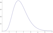
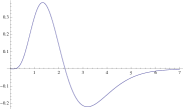
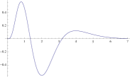
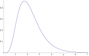
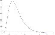
Figure 1 shows graphs of such kernels that correspond to the same value of the composed variance, using either a uniform distribution or a logarithmic distribution of the intermediate scale levels. Generally, these kernels are highly asymmetric for small values of $K$, whereas they become gradually more symmetric as $K$ increases. The degree of continuity at the origin and the smoothness of transition phenomena increase with $K$ such that coupling of $K\geq 2$ kernels in cascade implies a $C^{K-2}$-continuity of the temporal scale-space kernel. Specifically, the kernels based on a logarithmic distribution of the intermediate scale levels allow for faster temporal dynamics compared to the kernels based on a uniform distribution of the intermediate scale levels.

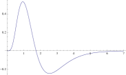
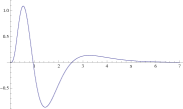
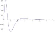
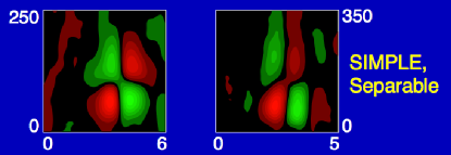
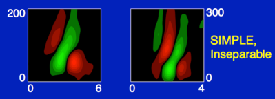
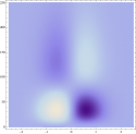
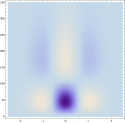
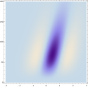
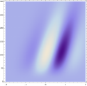
Figure 2 shows the result of modelling the spatio-temporal receptive fields of simple cells in V1 in this way, using the general idealized model of spatio-temporal receptive fields in equation (1) in combination with a temporal smoothing kernel obtained by coupling a set of first-order integrators/truncated exponential kernels in cascade. This result complements the general theoretical model for visual receptive fields in [12] with explicit modelling results and a theory for choosing and parameterizing the intermediate discrete temporal scale levels.

4 Temporal dynamics of the time-causal kernels

For the time-causal filters obtained by coupling truncated exponential kernels in cascade, there will be an inevitable temporal delay depending on the time constants $\mu_{k}$ of the individual filters. A straightforward way of estimating this delay is by using the additive property of mean values under convolution $m_{K}=\sum_{k=1}^{K}\mu_{k}$ according to (6). In the special case when all the time constants are equal $\mu_{k}=\sqrt{\tau/K}$, this measure is given by

$$m_{uni}=\sqrt{K\tau}$$ (12)

showing that the temporal delay increases if the temporal smoothing operation is divided into a larger number of smaller individual smoothing steps.

In the special case when the intermediate temporal scale levels are instead distributed logarithmically according to (8), with the individual time constants given by (9) and (10), this measure for the temporal delay is given by

$$\begin{split}m_{log}&=\frac{c^{-K}\left(c^{2}-\left(\sqrt{c^{2}-1}+1\right)c+\sqrt{c^{2}-1}\,c^{K}\right)}{c-1}\,\sqrt{\tau}\end{split}$$ (13)

with the limit value $m_{log-limit}=\lim_{K\rightarrow\infty}m_{log}=\frac{\sqrt{c^{2}-1}}{c-1}\sqrt{\tau}$ when the number of filters tends to infinity.

By comparing equations (12) and (13) including the limit value of the latter, we can specifically note that with increasing number of intermediate temporal scale levels, a logarithmic distribution of the intermediate scales implies shorter temporal delays than a uniform distribution of the intermediate scales.

Table 2 shows numerical values of these measures for different values of $K$ and $c$. As can be seen, the logarithmic distribution of the intermediate scales allows for significantly faster temporal dynamics than a uniform distribution.

Temporal mean values of time-causal kernels
$K$	$m_{uni}$	$m_{log}$ ($c=\sqrt{2}$)	$m_{log}$ ($c=2^{3/4}$)	$m_{log}$ ($c=2$)
2	1.414	1.414	1.399	1.366
3	1.732	1.707	1.636	1.549
4	2.000	1.914	1.777	1.641
5	2.236	2.061	1.860	1.686
6	2.449	2.164	1.910	1.709
7	2.646	2.237	1.940	1.721
8	2.828	2.289	1.957	1.732

Table 1: Numerical values of the temporal delay in terms of the temporal mean $m=\sum_{k=1}^{K}\mu_{k}$ in units of $\sigma=\sqrt{\tau}$ for time-causal kernels obtained by coupling $K$ truncated exponential kernels in cascade in the cases of a uniform distribution of the intermediate temporal scale levels $\tau_{k}=k\tau/K$ or a logarithmic distribution $\tau_{k}=c^{2(k-K)}\tau$ with $c>1$.

Temporal delays from the maxima of time-causal kernels
$K$	$t_{max,uni}$	$t_{max,log}$ ($c=\sqrt{2}$)	$t_{max,log}$ ($c=2^{3/4}$)	$t_{max,log}$ ($c=2$)
2	0.707	0.707	0.688	0.640
3	1.154	1.122	1.027	0.909
4	1.500	1.385	1.199	1.014
5	1.789	1.556	1.289	1.060
6	2.041	1.669	1.340	1.083
7	2.268	1.745	1.370	1.095
8	2.475	1.797	1.388	1.100

Table 2: Numerical values for the temporal delay of the local maximum in units of $\sigma=\sqrt{\tau}$ for time-causal kernels obtained by coupling $K$ truncated exponential kernels in cascade in the cases of a uniform distribution of the intermediate temporal scale levels $\tau_{k}=k\tau/K$ or a logarithmic distribution $\tau_{k}=c^{2(k-K)}\tau$ with $c>1$.

Additional temporal characteristics.

Because of the asymmetric tails of the time-causal temporal smoothing kernels, temporal delay estimation by the mean value may however lead to substantial overestimates compared to e.g. the position of the local maximum. To provide more precise characteristics in the case of a uniform distribution of the intermediate temporal scale levels, for which a compact closed form expression is available for the composed kernel

$$h_{composed}(t;\;\mu,K)=\frac{t^{K-1}\,e^{-t/\mu}}{\mu^{K}\,\Gamma(K)}$$ (14)

let us differentiate this function $\partial_{t}\left(h_{composed}(t;\;\mu,K)\right)=\frac{e^{-\frac{t}{\mu}}((K-1)\mu-t)\left(\frac{t}{\mu}\right)^{K+1}}{t^{3}\,\Gamma(K)}$ and solve for the positions of the local maximum

$$\begin{split}t_{max,uni}&=(K-1)\,\mu=\frac{(K-1)}{\sqrt{K}}\sqrt{\tau}.\end{split}$$ (15)

Table 2 shows numerical values for the position of the local maximum for both types of time-causal kernels. As can be seen from the data, the temporal response properties are significantly faster for a logarithmic distribution of the intermediate scale levels compared to a uniform distribution and the difference increases rapidly with $K$. These temporal delay estimates are also significantly shorter than the temporal mean values, in particular for the logarithmic distribution.

If we consider a temporal event that occurs as a step function over time (e.g. a new object appearing in the field of view) and if the time of this event is estimated from the local maximum over time in the first-order temporal derivative response, then the temporal variation in the response over time will be given by the shape of the temporal smoothing kernel. The local maximum over time will occur at a time delay equal to the time at which the temporal kernel has its maximum over time. Thus, the position of the maximum over time of the temporal smoothing kernel is highly relevant for quantifying the temporal response dynamics.

5 Computational implementation

The computational model for spatio-temporal receptive fields presented here is based on spatio-temporal image data that are assumed to be continuous over time. When implementing this model on sampled video data, the continuous theory must be transferred to discrete space and discrete time.

In this section we describe how the temporal and spatio-temporal receptive fields can be implemented in terms of corresponding discrete scale-space kernels that possess scale-space properties over discrete spatio-temporal domains.

5.1 Discrete temporal scale-space kernels based on recursive filters

Given video data that has been sampled by some temporal frame rate $r$, the temporal scale $\sigma_{t}$ in the continuous model in units of seconds is first transformed to a variance $\tau$ relative to a unit time sampling

$$\tau=r^{2}\,\sigma_{t}^{2}$$ (16)

where $r$ may typically be either 25 Hz or 50 Hz. Then, a discrete set of intermediate temporal scale levels $\tau_{k}$ is defined by (8) or (11) with the difference between successive scale levels according to $\Delta\tau_{k}=\tau_{k}-\tau_{k-1}$ (with $\tau_{0}=0$).

For implementing the temporal smoothing operation between two such adjacent scale levels (with the lower level in each pair of adjacent scales referred to as $f_{in}$ and the upper level as $f_{out}$), we make use of a first-order recursive filter

$$f_{out}(t)-f_{out}(t-1)=\frac{1}{1+\mu_{k}}\,(f_{in}(t)-f_{out}(t-1))$$ (17)

with generating function

$$H_{geom}(z)=\frac{1}{1-\mu_{k}\,(z-1)}$$ (18)

which is a time-causal kernel and satisfies discrete scale-space properties of guaranteeing that the number of local extrema or zero-crossings in the signal will not increase with increasing scale (Lindeberg [13]; Lindeberg and Fagerström [10]). Each such filter has temporal mean value $m_{k}=\mu_{k}$ and temporal variance $\Delta\tau_{k}=\mu_{k}^{2}+\mu_{k}$, and we compute $\mu_{k}$ from $\Delta\tau_{k}$ according to

$$\mu_{k}=\frac{\sqrt{1+4\Delta\tau_{k}}-1}{2}.$$ (19)

By the additive property of variances under convolution, the discrete variances of the discrete temporal scale-space kernels will perfectly match those of the continuous model, whereas the mean values and the temporal delays may differ somewhat. If the temporal scale $\tau_{k}$ is large relative to the temporal sampling density, the discrete model should be a good approximation in this respect.

By the time-recursive formulation of this temporal scale-space concept, the computations can be performed based on a compact temporal buffer over time, which contains the temporal scale-space representations at temporal scales $\tau_{k}$ and with no need for storing any additional temporal buffer of what has occurred in the past to perform the corresponding temporal operations.

5.2 Discrete implementation of spatial Gaussian smoothing

To implement the spatial Gaussian operation on discrete sampled data, we do first transform a spatial scale parameter $\sigma_{x}$ in units of e.g. degrees of visual angle to a spatial variance $s$ relative to a unit sampling density according to

$$s=p^{2}\sigma_{x}^{2}$$ (20)

where $p$ is the number of pixels per spatial unit e.g. in terms of degrees of visual angle at the image center. Then, we convolve the image data with the separable two-dimensional discrete analogue of the Gaussian kernel (Lindeberg [13])

$$T(n_{1},n_{2};\;s)=e^{-2s}I_{n_{1}}(s)\,I_{n_{2}}(s)$$ (21)

where $I_{n}$ denotes the modified Bessel functions of integer order and which corresponds to the solution of the semi-discrete diffusion equation

$$\partial_{s}L(n_{1},n_{2};\;s)=\frac{1}{2}(\nabla_{\times}^{2}L)(n_{1},n_{2};\;s)$$ (22)

where $\nabla_{\times}^{2}$ denotes the five-point discrete Laplacian operator defined by $(\nabla_{\times}^{2}f)(n_{1},n_{2})=f(n_{1}-1,n_{2})+f(n_{1}+1,n_{2})+f(n_{1},n_{2}-1)+f(n_{1},n_{2}+1)-4f(n_{1},n_{2})$. These kernels constitute the natural way to define a scale-space concept for discrete signals corresponding to the Gaussian scale-space over a symmetric domain in the sense of guaranteeing non-enhancement of local extrema, while also ensuring a semi-group property $T(\cdot,\cdot;\;s_{1})*T(\cdot,\cdot;\;s_{2})=T(\cdot,\cdot;\;s_{1}+s_{2})$ over the discrete domain which implies that representations at coarser scales can be computed from representations at finer scales using a cascade property.

This operation can be implemented either by explicit spatial convolution with spatially truncated kernels $\sum_{n_{1}=-N}^{N}\sum_{n_{2}=-N}^{N}T(n_{1},n_{2};\;s)>1-\varepsilon$ for small $\varepsilon$ of the order $10^{-8}$ to $10^{-6}$ with mirroring at the image boundaries (adiabatic boundary conditions) or using the closed-form expression of the Fourier transform $\varphi(\theta_{1},\theta_{2})=\sum_{n_{1}=-\infty}^{\infty}\sum_{n_{1}=-\infty}^{\infty}T(n_{1},n_{2};\;s)\,e^{-i(n_{1}\theta_{1}+n_{2}\theta_{2})}=e^{-2t(\sin^{2}(\frac{\theta_{1}}{2})+\sin^{2}(\frac{\theta_{2}}{2}))}$.

5.3 Discrete implementation of spatio-temporal receptive fields

For separable spatio-temporal receptive fields, we implement the spatio-temporal smoothing operation by separable combination of the spatial and temporal scale-space concepts in sections 5.1 and 5.2. From this representation, spatio-temporal derivative approximations are then computed from difference operators

$$\begin{split}\delta_{t}&=(-1,+1)\quad\quad\quad\delta_{tt}=(1,-2,1)\end{split}$$ (23)

$$\begin{split}\delta_{x}&=(-\frac{1}{2},0,+\frac{1}{2})\quad\quad\delta_{xx}=(1,-2,1)\end{split}$$ (24)

expressed over the appropriate dimension. From the general theory in (Lindeberg [15]) it follows that the scale-space properties for the original zero-order signal will be transferred to such derivative approximations, thereby implying theoretically well-founded implementation of discrete derivative approximations.

For non-separable spatio-temporal receptive fields corresponding to a non-zero image velocity $v=(v_{1},v_{2})^{T}$, we implement the spatio-temporal smoothing operation by first warping the video data $(x_{1}^{\prime},x_{2}^{\prime})^{T}=(x_{1}-v_{1}t,x_{2}-v_{2}t)^{T}$ using spline interpolation. Then, we apply separable spatio-temporal smoothing in the transformed domain and unwarp the result back to the original domain. Over a continuous domain, such an operation is equivalent to convolution with corresponding velocity-adapted spatio-temporal receptive fields, while being significantly faster in a discrete implementation than corresponding explicit convolution with non-separable receptive fields over three dimensions.

In addition to a transfer of the scale-space properties from the continuous model to the discrete implementation, all the components in this discretization, the discrete Gaussian kernel, the time-recursive filters and the discrete derivative approximations, can be seen as mathematical approximations of the corresponding continuous counterparts. Thereby, the behaviour of the discrete implementation will approach the corresponding continuous model.

6 Summary and discussion

We have presented an improved computational model for spatio-temporal receptive fields based on time-causal and time-recursive spatio-temporal scale-space representation defined from a set of first-order integrators or truncated exponential filters coupled in cascade over the temporal domain in combination with a Gaussian scale-space concept over the spatial domain. This model can be efficiently implemented in terms of recursive filters and we have shown how the continuous model can be transferred to a discrete implementation while retaining discrete scale-space properties. Specifically, we have analysed how remaining design parameters within the theory, in terms of the number of first-order integrators coupled in cascade and a distribution parameter of a logarithmic distribution, affect the temporal response dynamics in terms of temporal delays.

Compared to other spatial and temporal scale-space representations based on continuous scale parameters, a conceptual difference with the temporal scale-space representation underlying the proposed spatio-temporal receptive fields, is that the temporal scale levels have to be discrete. Thereby, we sacrifice scale invariance as resulting from Gaussian scale-space concepts based on causality or non-enhancement of local extrema (Koenderink [16]; Lindeberg [11]) or used as a scale-space axiom in certain axiomatic scale-space formulations (Iijima [17]; Florack et al. [18]; Pauwels et al. [19]; Weickert et al. [20]; Duits et al. [21]; Fagerström [22]); see also Koenderink and van Doorn [23], Florack et al. [24] and Tschirsich and Kuijper [25] for other scale-space approaches closely related to this work. For a vision system intended to operate in real time using no other explicit storage of visual data from the past than a compact time-recursive buffer of spatio-temporal scale-space at different temporal scales, the loss of a continuous temporal scale parameter may however be less of a practical constraint, since one would anyway have to discretize the temporal scale levels in advance to be able to register the image data to perform any computations at all.

In the special case when all the time constants of the first-order integrators are equal, the resulting temporal smoothing kernels in the continuous model (14) correspond to Laguerre functions, which have been previously used for modelling the temporal response properties of neurons in the visual system (den Brinker and Roufs [26]) and for computing spatio-temporal image features in computer vision (Rivero-Moreno and Bres [27]; Berg et al. [28]). Regarding the corresponding discrete model with all time constants equal, the corresponding discrete temporal smoothing kernels approach Poisson kernels when the number of temporal smoothing steps increases while keeping the variance of the composed kernel fixed (Lindeberg and Fagerström [10]). Such Poisson kernels have also been used for modelling biological vision (Fourtes and Hodgkin [29]). Compared to the special case with all time constants equal, a logarithmic distribution of the intermediate temporal scale levels (8) does on the other hand allow for larger flexibility in the trade-off between temporal smoothing and temporal response characteristics, specifically enabling faster temporal responses (shorter temporal delays) and higher computational efficiency when computing multiple temporal or spatio-temporal receptive field responses involving coarser temporal scales.

References

- [1] Hubel, D.H., Wiesel, T.N.: Brain and Visual Perception: The Story of a 25-Year Collaboration. Oxford University Press (2005)
- [2] DeAngelis, G.C., Ohzawa, I., Freeman, R.D.: Receptive field dynamics in the central visual pathways. Trends in Neuroscience 18 (1995) 451–457
- [3] DeAngelis, G.C., Anzai, A.: A modern view of the classical receptive field: Linear and non-linear spatio-temporal processing by V1 neurons. In: Chalupa, L.M., Werner, J.S., eds.: The Visual Neurosciences vol 1. MIT Press (2004) 704–719
- [4] Adelson, E., Bergen, J.: Spatiotemporal energy models for the perception of motion. J. Optical Society of America A 2 (1985) 284–299
- [5] Zelnik-Manor, L., Irani, M.: Event-based analysis of video. In: Proc. Computer Vision and Pattern Recognition, Kauai Marriott, Hawaii (2001) II:123–130
- [6] Laptev, I., Lindeberg, T.: Local descriptors for spatio-temporal recognition. In: ECCV’04 Workshop on Spatial Coherence for Visual Motion Analysis. Springer LNCS vol 3667 (2004) 91–103
- [7] Jhuang, H., Serre, T., Wolf, L., Poggio, T.: A biologically inspired system for action recognition. In: Int. Conf. on Computer Vision (2007) 1–8
- [8] Shabani, A.H., Clausi, D.A., Zelek, J.S.: Improved spatio-temporal salient feature detection for action recognition. In: British Machine Vision Conf. (2011) 1–12
- [9] Fleet, D.J., Langley, K.: Recursive filters for optical flow. IEEE Trans. Pattern Analysis and Machine Intell. 17 (1995) 61–67
- [10] Lindeberg, T., Fagerström, D.: Scale-space with causal time direction. In: European Conf. on Computer Vision. Springer LNCS vol 1064 (1996) 229–240
- [11] Lindeberg, T.: Generalized Gaussian scale-space axiomatics comprising linear scale-space, affine scale-space and spatio-temporal scale-space. J. of Mathematical Imaging and Vision 40 (2011) 36–81
- [12] Lindeberg, T.: A computational theory of visual receptive fields. Biological Cybernetics 107 (2013) 589–635
- [13] Lindeberg, T.: Scale-space for discrete signals. IEEE Trans. Pattern Analysis and Machine Intell. 12 (1990) 234–254
- [14] Koenderink, J.J.: Scale-time. Biological Cybernetics 58 (1988) 159–162
- [15] Lindeberg, T.: Discrete derivative approximations with scale-space properties: A basis for low-level feature extraction. J. Math. Imaging Vision 3 (1993) 349–376
- [16] Koenderink, J.J.: The structure of images. Biol. Cyb. 50 (1984) 363–370
- [17] Iijima, T.: Observation theory of two-dimensional visual patterns. Papers of Technical Group on Automata and Automatic Control, IECE, Japan (1962)
- [18] Florack, L.M.J., ter Haar Romeny, B.M., Koenderink, J.J., Viergever, M.A.: Scale and the differential structure of images. Image Vision Comp. 10 (1992) 376–388
- [19] Pauwels, E.J., Fiddelaers, P., Moons, T., van Gool, L.J.: An extended class of scale-invariant and recursive scale-space filters. IEEE Trans. Pattern Analysis and Machine Intell. 17 (1995) 691–701
- [20] Weickert, J., Ishikawa, S., Imiya, A.: On the history of Gaussian scale-space axiomatics. In: Gaussian Scale-Space Theory, Springer (1997) 45–59
- [21] Duits, R., Florack, L., de Graaf, J., ter Haar Romeny, B.: On the axioms of scale space theory. J. of Mathematical Imaging and Vision 22 (2004) 267—298
- [22] Fagerström, D.: Spatio-temporal scale-spaces. In: Scale-Space and Variational Methods in Computer Vision. Springer LNCS vol 4485 (2007) 326–337
- [23] Koenderink, J.J., van Doorn, A.J.: Receptive field families. Biological Cybernetics 63 (1990) 291–298
- [24] Florack, L.M.J., ter Haar Romeny, B.M., Koenderink, J.J., Viergever, M.A.: Families of tuned scale-space kernels. In ECCV’92 Springer LNCS vol 588 (1992) 19–23
- [25] M. Tschirsich, M., Kuijper: Notes on discrete Gaussian scale space. J. of Mathematical Imaging and Vision 51 (2015) 106–123
- [26] den Brinker, A.C., Roufs, J.A.J.: Evidence for a generalized Laguerre transform of temporal events by the visual system. Biological Cybernetics 67 (1992) 395–402
- [27] Rivero-Moreno, C.J., Bres, S.: Spatio-temporal primitive extraction using Hermite and Laguerre filters for early vision video indexing. In: Image Analysis and Recognition. Springer LNCS vol 3211 (2004) 825–832
- [28] van der Berg, E.S., Reyneke, P.V., de Ridder, C.: Rotational image correlation in the Gauss-Laguerre domain. In: SPIE vol 9257. (2014) 92570F–1–92570F–17
- [29] Fourtes, M.G.F., Hodgkin, A.L.: Changes in the time scale and sensitivity in the omatadia of limulus. Journal of Physiology 172 (1964) 239–263