Euclid Asteroseismology and Kuiper Belt Objects

1 Introduction

In two earlier papers, we pointed out that WFIRST microlensing observations toward the Galactic bulge would automatically yield a treasure trove of asteroseismic (Gould et al., 2015) and Kuiper Belt Object (KBO) (Gould, 2014) data. These papers contained detailed analytic calculations that permit relatively easy scaling to other missions and experiments. One very relevant mission is Euclid, which is presently scheduled to be launched in 2020. Unlike WFIRST, Euclid does not yet have a microlensing component, but such a component is being actively discussed.

Based on a most naive assessment, Euclid would appear to be much less effective in extracting non-microlensing science from microlensing data than WFIRST. Euclid has 1/2 the telescope diameter of WFIRST, 2.7 times larger linear pixel scale, 1/4 as many visits to each target, and 1/2 the angular area of the survey.

However, as we show, such naive assessment would be quite wrong since Euclid will be able to detect oscillations in giants that are about 0.8 mag brighter than for WFIRST, i.e., to about 0.8 mag above the red clump. Hence, it will obtain asteroseismic measurements for roughly 100,000 stars.

For KBOs, Euclid benefits greatly by having an optical channel in addition to its primary infrared (IR) channel, even though it is expected that the optical exposure time will be 3 times smaller than for the IR. The optical observations gain substantially from their smaller point spread function (PSF) as well as the fact that KBOs (unlike stars) do not suffer extinction. Hence, Euclid will also be a powerful probe of KBOs.

2 Euclid Characteristics

We adopt Euclid survey characteristics from Penny et al. (2013), with some slight (and specified) variations. In each case, for easy reference, we place the corresponding assumed WFIRST parameters in parentheses. Mirror diameter $D=1.2\,$m ($2.4\,$m); pixel size $p=0.3^{\prime\prime}$ ($0.11^{\prime\prime}$), detector size 8k$\times$8k (16k$\times$16k), median wavelength $\lambda=1.7\,\mu$m ($1.5\,\mu$m), photometric zero point $H_{\rm vega}=23.5$ (26.1), exposure time 52s (52s), effective background (including read noise, $H_{{\rm vega},\rm sky}=20.0\,\rm arcsec^{-2}$, and dark current) $209\,e^{-}$ ($341\,e^{-}$), full pixel well $n_{\rm max}=10^{5}$ ($10^{5}$), and single read time $t_{\rm single}=2.6\,$s ($t_{\rm single}=2.6\,$s). In fact, Penny et al. (2013) do not specify a read time, so we use the same value as for WFIRST to simplify the comparison. Also, Penny et al. (2013) adopt an exposure time of 54 s, but we use 52 to again simplify the comparison. Finally, Penny et al. (2013) list $n_{\rm max}=2^{16}$, but this appears to be in error. In any case, since the detector is very similar to WFIRST, these two numbers should be the same.

In our calculations we first consider simple 52 s exposures, but later take account of the fact that five such exposures will be carried out in sequence over $\sim 285\,$s.

3 Asteroseismology

3.1 Bright-star photometry

From Equation (16) of Gould et al. (2015), the fractional error (statistical) in the log flux $F$ (essentially, magnitude error) is

$$\sigma(\ln F)=[\pi n_{\rm max}(3-Q)]^{-1/2}r_{\rm unsat}^{-1};\quad r_{\rm unsat}\equiv{\theta_{\rm unsat}\over p}$$ (1)

where $p$ is the pixel size, $\theta_{\rm unsat}$ is the radius of the closest unsaturated pixel (in the full read), $n_{\rm max}$ is the full well of the pixel,

$$Q=N_{\rm read}^{-1}+3(2N_{\rm read})^{-2/3},$$ (2)

and $N_{\rm read}$ is the number of non-destructive reads.

When comparing WFIRST and Euclid, the most important factor is $r_{\rm unsat}$. To determine how this scales with mirror size, pixel size, exposure time $t$, throughput $f$, and mean wavelength $\lambda$, we adopt a common PSF function of angle $\theta$, $A(D\theta/\lambda)$, which is scaled such that $\int dx2\pi xA(x)\equiv 1$. Then, if a total of $K$ photons fall on the telescope aperture, the number falling in a pixel centered at $\theta$ is

$$n_{\rm pixel}=p^{2}KfA(D\theta/\lambda)(D/\lambda)^{2}$$ (3)

Setting $n_{\rm pixel}=n_{\rm max}$, we derive

$$r_{\rm unsat}={A^{-1}[n_{\rm max}\lambda^{2}/(KfD^{2}p^{2})]\over pD/\lambda}.$$ (4)

Then noting that $K=kfN_{\rm read}t_{\rm single}D^{2}$, where $k$ is a constant, we obtain

$$r_{\rm unsat}={A^{-1}[n_{\rm max}\lambda^{2}/(kft_{\rm single}N_{\rm read}D^{4}p^{2})]\over pD/\lambda}$$ (5)

Finally, noting that in the relevant range, a broad-band Airy profile scales $A(x)\propto x^{-3}$, we find a ratio of Euclid (E) to WFIRST (W) unsaturated radii,

$${r_{{\rm unsat},E}\over r_{{\rm unsat},W}}=\biggl{[}{(N_{\rm read}D\lambda f/p)_{E}\over(N_{\rm read}D\lambda f/p)_{W}}\biggr{]}^{1/3}\simeq 0.42.$$ (6)

In making this evaluation we note that $(D_{E}/D_{W})=0.50$, $(p_{E}/p_{W})=2.73$, $(\lambda_{E}/\lambda_{W})=1.13$, and $(f_{E}/f_{W})=10^{0.4(23.52-26.1)}/(D_{E}/D_{W})^{2}=0.365$. The last number may be somewhat surprising. It derives mainly from WFIRST’s broader passband ($1\,\mu$m vs. $0.6\,\mu$m and its gold-plated (so infrared optimized) mirror. The other ratio of factors is

$${3-Q_{E}\over 3-Q_{W}}=1.$$ (7)

Therefore, we conclude that in the regime that the central pixel is saturated in a single read, a sequence of 5 Euclid exposures (requiring about 285 s including readout) yields a factor 1.06 increase in photometric errors compared to a single WFIRST exposure (lasting 52 s).

However, whereas this regime applies to stars $H<11.6$ for WFIRST ($x$-intercept of lower curve of middle panel in Figure 1 of Gould et al. 2015), this break occurs at a brighter value for Euclid. To evaluate this offset, we rewrite Equation (3): $N_{\rm pixel}=kfN_{\rm read}t_{\rm single}(D^{2}p/\lambda)^{2}A(rDp/\lambda)$. Hence, the offset (at fixed $r$) between the break points on the WFIRST and Euclid diagrams is

$$\Delta H=-2.5\log{[fD\lambda/p]_{E}/[fD\lambda/p]_{H}}=2.8$$ (8)

That is, this boundary occurs at $H=11.6-\Delta H=8.8$, which is significantly brighter than the majority of potential asteroseismic targets. However, inspection of that Figure shows that the same scaling ($\sigma\propto F_{H}^{-1/3}$) applies on both sides of the $H=11.6$ “boundary”. The reason for this is quite simple. As we consider fainter source stars $F_{H}$, the saturated region of course continues to decline. Since the Airy profile at large radii scales as $A(x)\propto x^{-3}$, the radius of this region scales as $r_{\rm unsat}\propto F_{H}^{1/3}$. Hence, the number of semi-saturated pixels (each contributing $n_{\rm max}$ to the total photon counts) scales $\propto F_{H}^{2/3}$, which implies that the fractional error scales $\propto F_{H}^{-1/3}$. This breaks down only at (or actually, close to) the point that the central pixel is unsaturated in a full read (at which point the error assumes standard $\propto F_{H}^{-1/2}$ scaling). That is, in the case of Euclid, the $F_{H}^{-1/3}$ scaling applies to about $H<14.8-\Delta H=12.0$, which is still toward the bright end of potential targets.

3.2 Bright-star astrometry

From Gould et al. (2015)

$$\sigma(\theta)={p\over\sqrt{3\pi n_{\rm max}\ln(1.78N_{\rm read}+0.9)}},$$ (9)

in the saturated regime. Hence, using the same parameters (for a single Euclid sub-exposure)

$${\sigma(\theta)_{E}\over\sigma(\theta)_{W}}=2.73.$$ (10)

Then taking account of the fact that Euclid has five such sub-exposures, we obtain $\sigma(\theta)_{E}/\sigma(\theta)_{W}=1.22$, i.e., Euclid is very similar to WFIRST.

However, as in the case of photometric errors, the boundary of the regime to which this applies is $H<8.8$ for Euclid (compared to $H<11.6$ for WFIRST). And, more importantly, for astrometric errors, the functional form of errors does in fact change beyond this break (see Figure 1 of Gould et al. 2015).

The reason for this change in form of astrometric errors can be understood by essentially the same argument given for the form of photometric errors in the previous section. In the regime between saturation of the central pixel in one read and $N_{\rm read}$ reads, the region $r<r_{\rm unsat}\propto F_{H}^{1/3}$ dominates the astrometric signal. For astrometric signals, each pixel contributes to the (S/N)² as $n_{\rm max}/r^{2}$, and therefore the entire region contributes

$$\biggl{(}{\rm S\over N}\biggr{)}^{2}\propto\int_{1}^{r_{\rm unsat}}{rdr\over r^{2}}=\ln r_{\rm unsat};\qquad r_{\rm unsat}\propto F_{H}^{1/3}$$ (11)

Hence, between these two limits ($11.6<H<14.8$ for WFIRST and $8.8<H<12$ for Euclid) the astrometric errors should scale $\sigma\propto(\ln F^{1/3})^{-1/2}\propto(\ln F)^{-1/2}$. That is, these errors should increase by a factor $\sqrt{\ln N_{\rm read}}=1.73$, which is indeed very similar to what is seen in Figure 1 of Gould et al. 2015.

3.3 Analytic Error Estimates for Bright Euclid Stars

We summarize the results of Sections 3.1 and 3.2 in the form of analytic expressions for the photometric and astrometric errors for bright stars as a function of magnitude for single-epoch Euclid observations consisting of 5 52-second exposures. The photometric errors are,

$$\sigma_{\rm phot} = 0.47\,{\rm mmag}\,10^{(2/15)(H-12)},\ (H<12)$$

$$\sigma_{\rm phot} = 0.47\,{\rm mmag}\,10^{(1/5)(H-12)},\ (H>12)$$ (12)

The astrometric errors are

$$\sigma_{\rm ast} = 73\,{\mu\rm as}\quad(4.4<H<8.8)$$

$$\sigma_{\rm ast} = 73\,{\mu\rm as}\,\sqrt{{\ln 10\over 2.5}(H-8.8)+1}\quad(8.8<H<12)$$

$$\sigma_{\rm ast} = 145\,{\mu\rm as}\,10^{(1/5)(H-12)}\quad(H>12)$$ (13)

Parameter	KIC 2437965	KIC 2425631	KIC 2836038
$T_{\rm eff}$ (K)	4356	4568	4775
$\log g$ (cgs)	1.765	2.207	2.460
$\rm[Fe/H]$ (dex)	0.43	$-0.10$	0.33
$R(R_{\odot})$	24.94	16.44	11.28
$M_{H}$ (mag)	$-3.14$	$-2.38$	$-1.60$
$A_{H}/A_{Kp}$	0.45	0.45	0.45
$\sigma_{E}$ (mmag)	0.483	0.685	0.984
Reference	P14	P14	C14

Table 1: Fundamental properties and simulation parameters for Euclid simulations. P14 = Pinsonneault et al. (2014), C14 = Casagrande et al. (2014).

3.4 Asteroseismic Simulations for Euclid

As for WFIRST, we evaluate the asteroseismic capabilities of Euclid by its ability to recover the frequency of maximum power $\nu_{\rm max}$ and the large frequency separation $\Delta\nu$. Both are key quantities that can be used to estimate radii and masses for large ensembles of giants, as demonstrated with the Kepler sample (e.g., Kallinger et al. 2010; Hekker et al. 2011; Mosser et al. 2012).

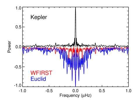
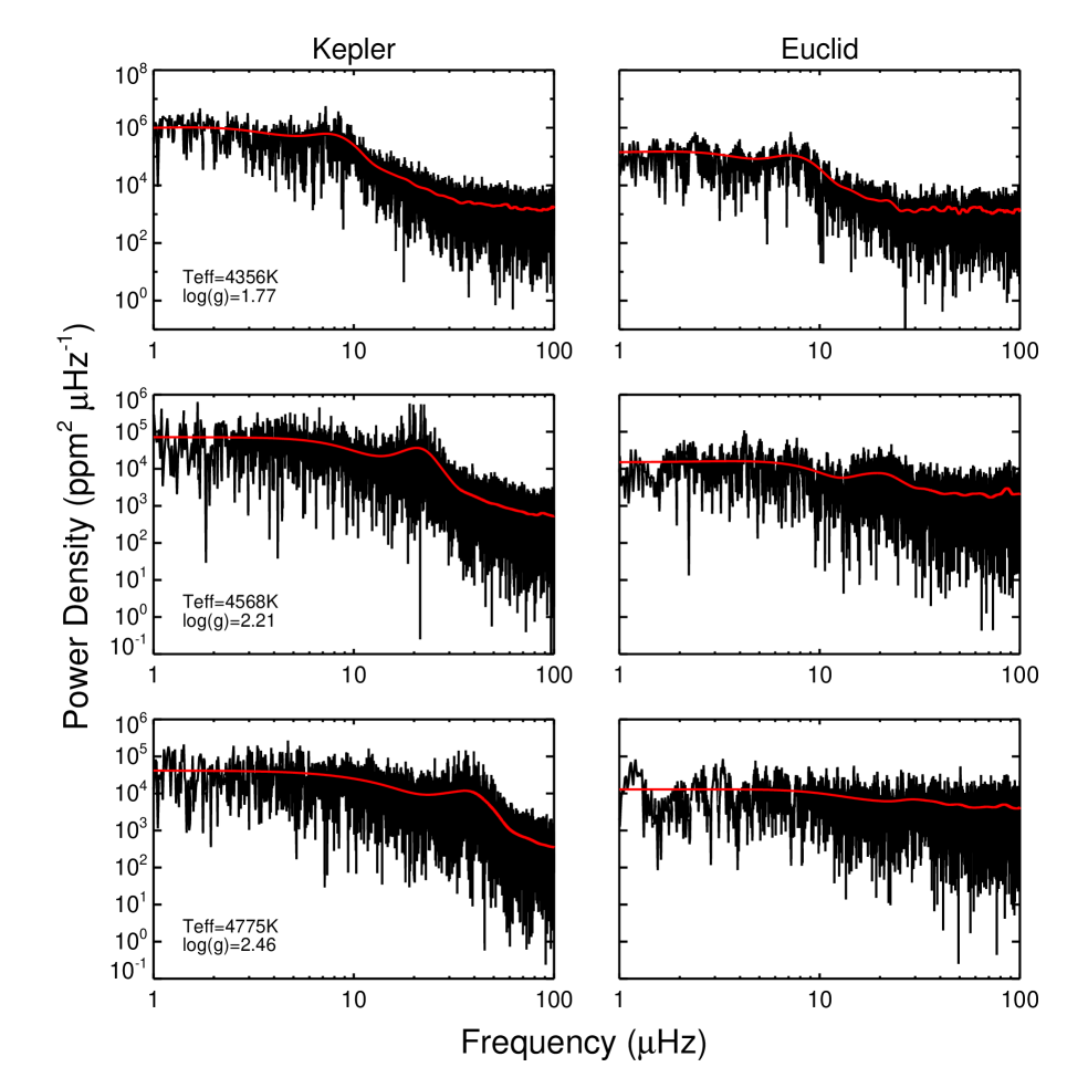
Figures 1, 2, are the Euclid analogs of Figures 3, and 4 from Gould et al. (2015) for WFIRST, while Figure 3 illustrates the same physics as Figure 5 from Gould et al. (2015). In addition to incorporating the analytic formulae summarized in Section 3.3, they also take account of the following assumptions about the Euclid microlensing observations. First, they assume an 18 minute observing cycle (compared to 15 minutes for WFIRST). Second, they assume four 30-day observing campaigns (compared to six 72-day campaigns for WFIRST). Finally, we adopt a specific “on-off” (bold, normal) schedule of (30,124,30,335,30,181,30) days. This schedule has been chosen to be consistent with the Euclid sun-exclusion angle and to have two campaigns in each of the spring and autumn (useful for parallaxes) but is otherwise arbitrary.

The area under the spectral window function in Figure 1 is about 2.4 times larger than for WFIRST due to the fact that the campaigns are a factor $72/30=2.4$ times shorter. Nevertheless, the FWHM of this envelope is still only about 500 nHz, which is far less than the $\nu_{\rm max}\sim 8\,\mu$Hz for the brightest star shown in Figure 2. Hence, it is only for extremely bright stars that the width of this envelope will degrade the measurement of $\nu_{\rm max}$.

Figure 2 is qualitatively similar to Figure 4 from Gould et al. (2015). Note that as for the WFIRST simulations, the Kepler time series has been shorted to the assumed full duration (with gaps, 760 days) of the Euclid run to allow a direct comparison of the effects of sampling. As shown in Sections 3.1 and 3.3, the individual photometric measurements have very similar precision for WFIRST and Euclid in the relevant magnitude range. However, Euclid has a factor $(18/15)\times(72/30)\times(6/4)=4.0$ times fewer of them, which leads to a factor 2.0 less sensitivity. This means that the “noise floor” kicks in at a power density of about $10^{3.3}\,\rm ppm^{2}\,\mu Hz^{-1}$ rather than $10^{3.0}$. This is the reason that in the bottom panel, the $\nu_{\rm max}$ peak is not visible above the floor, whereas for WFIRST it is robustly visible (middle panel of Figure 4 of Gould et al. 2015). On the other hand, the $\nu_{\rm max}$ peak in the top panel is about equally robust in simulated WFIRST and Euclid data. The middle panel represents the approximate limit of Euclid’s ability to measure $\nu_{\rm max}$.

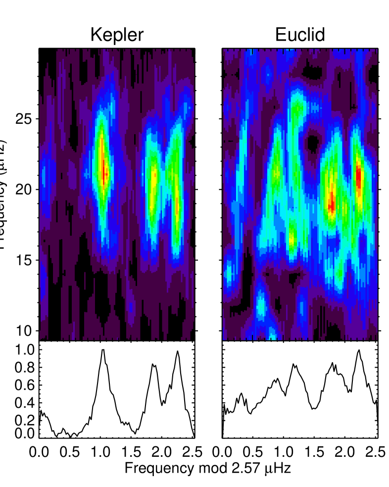
Figure 3 is an échelle diagram for the spectrum shown in the middle panel of Figure 2, i.e., the one just described that is at the limit of Euclid’s ability to measure $\nu_{\rm max}$. Figure 3 shows that this star is also just above the limit of Euclid’s ability to measure the other key asteroseismic parameter, the large frequency spacing $\Delta\nu$. In these diagrams, the abscissa designates frequency modulo the adopted $\Delta\nu$, while the ordinate is frequency. Hence, they represent the power spectrum divided into $\Delta\nu$-wide bins and stacked one above the other. If the adopted $\Delta\nu$ is correct (and the data are of sufficient quality) then the diagram should look like a series of vertical streaks, one for each mode degree $(l=1,2,0)$ comprising a series of overtones. This is clearly the case for the original Kepler data. While the ridges in the simulated Euclid data are heavily smeared out due to the window function, an identification of the correct $\Delta\nu$ is still possible. Hence both $\nu_{\rm max}$ and $\Delta\nu$ are measurable for this star. These quantities should also be measurable for brighter giants because these have both larger amplitude oscillations and smaller photometric errors, although for the most luminous giants the frequency resolution for a typical Euclid observing run will be too low to resolve $\Delta\nu$.

Figure 1: Spectral window function for a typical Kepler time series (top panel, black) and after degrading the time series to a typical duty cycle expected for Euclid and WFIRST (bottom panel, blue, red). Note that while the Euclid peak is much broader than for Kepler the power is still contained within $\sim 0.5\,\mu$Hz, which is substantially narrower than most spectral features of interest for most stars.

Figure 2: Power spectra of Kepler observations (left panels) and simulated Euclid observations (right panels) for three red giants in different evolutionary stages: high-luminosity red giant (top panels), 0.8 mag above red clump (middle panels) and red clump star (bottom panels). Red lines show the power spectra smoothed with a Gaussian with a full-width half-maximum of $2\Delta\nu$. Estimated stellar properties are given in the left panels, with a more complete description given in Table 1.

Figure 3: Échelle diagram for KIC 2425631 (corresponding to middle panel of Figure 2) for Kepler (left) and simulated Euclid (right) data. The abscissa is the frequency offset relative to the beginning of each order, which are separated by (an adopted) large-frequency spacing $\Delta\nu=2.57\,\mu$Hz. Hence, for example, at the frequency of maximum power $\nu_{\rm max}\sim 20\,\mu$Hz, the ordinate corresponds to the eighth order. In the Kepler échelle, the three mode degrees $l=1,2,0$ from left to right are easily discerned, which is not true of the Euclid échelle. However, the Euclid échelle does display clear vertical “streaking” which is the signature that the adopted $\Delta\nu=2.57\,\mu$Hz is the correct one.

3.5 Role of Euclid Parallaxes

In Gould et al. (2015), we argued that WFIRST parallaxes could help resolve ambiguities in the measurement of $\Delta\nu$ due to aliasing. That is, from color-surface brightness relations, one approximately knows the angular radius, which combined with the measured parallax, gives the physical radius $R$. By combining $R$, $\nu_{\rm max}$, and general scaling relations, one can approximately predict $\Delta\nu$, and so determine which of the alias-peaks should be centroided to find a more precise value.

However, this does not work for Euclid. From Equation (13) and the fact that there are a total of $\sim 10,000$ observations, it follows that the parallax errors are

$$\sigma(\pi) = 8\,{\mu\rm as}\,\sqrt{{\ln 10\over 2.5}(H-8.8)+1}\quad(8.8<H<12)$$

$$\sigma(\pi) = 15\,{\mu\rm as}\,10^{(1/5)(H-12)}\quad(H>12)$$ (14)

Hence, at the brightness of targets near the boundary of measurability, $H\sim 13$, the parallax errors are roughly 20%, which provides essentially no information. Even for the rarer targets at $H\sim 12$, the parallax measurements do little more than confirm that the star is in the bulge, which is already basically known in most cases. Nevertheless, these parallaxes are substantially better than Gaia parallaxes for the same stars and so could be useful for other purposes.

4 Kuiper Belt Objects

Gould (2014) carried out analytic calculations to assess how well WFIRST could detect and characterize Kuiper Belt Objects (KBOs), including orbits, binarity, and radii. Here we apply these analytic formulae to Euclid.

In contrast to WFIRST, Euclid will observe in two channels simultaneously, using an optical/IR dichroic beam-splitter. Because the microlensing targets will be heavily extincted in the optical, and also because bandwidth considerations restrict the optical downloads to once per hour (vs. once per 18 minutes for the IR), the optical data will provide only supplementary information for microlensing events. Similarly, for the heavily reddened (and intrinsically red) asteroseismology targets, the optical images will also be of secondary importance, and so were not considered in Section 3. However, KBOs lie in front of all the dust and hence both the optical and IR channels should be considered.

4.1 Euclid IR Observations of KBOs

We remind the reader that, in contrast to asteroseismology targets, KBOs are below the sky level and therefore are in a completely different scaling regime. In order to make use of the analytic formulae of Gould (2014), we first note that the Euclid point spread function (PSF) is slightly more undersampled than that of WFIRST by a factor $(0.30/0.11)\times(1.2/2.4)\times(1.5/1.7)=1.2$. We therefore adopt an effective sky background of $6B$, where $B=209\,e^{-}$ is the effective background in a single pixel (compared to $3B$ for the oversampled limit). That is, $H_{\rm sky}=23.5-2.5\log(6B/52)=20$, i.e., 1.7 mag brighter than for WFIRST. Then, following Equation (3) of Gould (2014), we estimate the astrometric precision of each measurement as

$$\sigma_{\rm ast}=\sqrt{2}{\sigma_{\rm psf}\over{\rm SNR}}={\rm 212\,mas\over SNR},$$ (15)

i.e., exactly twice the value for WFIRST (because the mirror is two times smaller). Here, the signal-to-noise ratio (SNR) of 5 co-added consecutive observations is given by

$${\rm SNR}=10^{0.4(H_{\rm zero}-H)},\qquad H_{\rm zero}=22.6.$$ (16)

Comparing this to Equation (1) of Gould (2014), we see that $H_{\rm zero}$ is 3.5 mag brighter than for WFIRST.

Before continuing, we remark on the issue of smeared images, which is potentially more severe for Euclid than WFIRST because the full duration of the 5 co-added exposures is about 5.5 times longer than the WFIRST exposure. However, due to the shorter duration of the observing window and the fact that this window has one end roughly at quadrature (and the other 30 days toward opposition), the typical relative velocities of the KBO and satellite are only about $5\,{\rm km}\,{\rm s}^{-1}$, which corresponds to $\sim 10\,{\mu\rm as}\,{\rm min}^{-1}$, which is still too small to substantially smear out the PSF, even in $\sim 5\,$min exposures.

Although the area of the Euclid field is only about half the size of the WFIRST field, the fact that the campaign duration is only 40% as long together with the very slow mean relative motion of the KBOs (previous paragraph) implies that this is even less of an issue than for WFIRST, which Gould (2014) showed was already quite minor. We therefore ignore it.

As with WFIRST, we assume that only 90% of the observations are usable, due to contamination of the others by bright stars. This balances the opposite impact of two effects: larger pixels increase the chance that a given bright star lands on the central pixel, while brighter $H_{\rm zero}$ decreases the pool of bright stars that can contribute to contamination. We also assume that 10% of the observing time is spent on other bands. These will provide important color information but are difficult or impossible to integrate into initial detection algorithms. Hence the total number of epochs per campaign is $N_{\rm cam}=1920$, i.e., a factor $\sim 3$ smaller than for WFIRST.

To determine the minimum total SNR required for a detection, we must determine the number of trials. We begin by rewriting Equation (18) of Gould (2014) as

$$N_{\rm try}=7\times 10^{14}\biggl{(}{\Delta t\over{\rm day}}\biggr{)}^{5}\biggl{(}{N_{\rm pix}\over 3\times 10^{9}}\biggr{)}\biggl{(}{\theta_{\rm pix}\over 110\,{\rm mas}}\biggr{)}^{-4}$$ (17)

where $N_{\rm pix}=3\times 8000^{2}=2\times 10^{8}$ is the total number of pixels in 3 Euclid fields, $\Delta t=30\,$day is the duration of a Euclid campaign, and $\theta_{\rm pix}=300\,$mas is the size of a Euclid pixel. Therefore $N_{\rm try}=2\times 10^{19}$. This is almost five orders of magnitude smaller than the corresponding number for WFIRST. Hence, the challenges posed by limitations of computing power that were discussed by Gould (2014) are at most marginally relevant for Euclid. Therefore, we ignore them here.

Then to find the limiting SNR at which a KBO can be detected, we solve Equation (17) from Gould (2014), i.e.,

$${\rm SNR}\gtrsim N_{\rm cam}^{-1/2}\sqrt{2\ln{N_{\rm try}\over{\rm SNR}}-\ln N_{\rm cam}}=0.22,$$ (18)

where $N_{\rm cam}$ is the of observations during a single-season observing campaign. Hence, the limiting magnitude is $H\lesssim 24.2$.

4.2 Euclid Optical Observations of KBOs

To compare optical with IR observations, we first note that the field of view is the same, but with pixels that are smaller by a factor 3. This means that the optical data are nearly critically sampled (100 mas pixels and 180 mas FWHM). The “RIZ” band is centered in $I$ band and has a flux zero point of $I_{\rm vega}=25.1$. As noted above, band-width constraints limit the number of optical images that can be downloaded (in addition to the primary IR images) to one per hour (for each of the three fields).

Taking into account the read noise of $4.5\,e^{-}$, a sky background of $I=21.0\,\rm arcsec^{-2}$, and the nearly critical sampling, we find the analog of Equation (16) to be

$${\rm SNR}=10^{0.4(I_{\rm zero}-I)},\qquad I_{\rm zero}=27.4$$ (19)

for 270 s exposures. Even allowing for the fact that there are only 30% as many $I$-band observations and that the typical color of a KBO is $I-H\sim 1$, this still represents an improvement of $27.4-22.6-1+2.5\log(0.3)=2.5$ magnitudes relative to $H$ band. Thus, the $I$-band observations will be the primary source of information about KBOs and we henceforth focus on these.

An important benchmark for understanding the relative sensitivity of WFIRST and Euclid is that at the KBO luminosity function break ($R=26.5$, $I=26.0$, $H=25.1$), we have SNR$\sim 2.5$ for WFIRST and SNR$\sim 3.6$ for Euclid.

For fixed field size and $\Delta t$, the number of trials (Eq. (17)) scales $N_{\rm try}\propto\theta_{\rm pix}^{-6}$, i.e., $N_{\rm try}\sim 10^{22}$, a factor $10^{2.9}$ higher for the optical than the IR. This implies that reaching the theoretical detection limit will require roughly $10^{26}$ floating point operations (FLOPs). While this is three orders of magnitude lower than WFIRST, it is not trivially achieved (Gould, 2014). For the moment we evaluate the detection limit assuming that it can be achieved and then qualify this conclusion further below. Assuming that 10% of observations are lost to bright stars and then solving Equation (18) yields SNR$\gtrsim 0.39$, i.e., a detection limit of $I\lesssim 28.4$. Considering that the break in the KBO luminosity function is $R\sim 26.5$ and that typically $R-I\sim 0.45$, this is about 1.5 mag below the break. Hence, Euclid optical observations will be a powerful probe of KBOs.

4.3 Detections

The main characteristics of the Euclid optical KBO survey can now be evaluated by comparing to the results of Gould (2014). The total number detected up to the break (and also the total number detected per magnitude between the break and the faint cutoff) will be $(4/6)/2.1=32\%$ smaller than for WFIRST (Figure 4 from Gould 2014) because there are 4 campaigns (rather than 6) and the survey area is a factor 2.1 times smaller.

Thus, there will be a total of 400 KBOs discovered that are brighter than the break and 530 per magnitude fainter than the break. In fact, this distribution is only known to be flat for about 1.5 mag. Euclid observations will reach about 2.4 mag below the break, provided that the computational challenges can be solved. However, as we discuss in Section 4.7, even if they cannot be solved, this will pull back the magnitude limit by only a few tenths.

Hence, Euclid will discover at least 800 KBOs down to the point that the KBO luminosity function is measured, and perhaps a few hundred beyond that.

4.4 Orbital Precision

To determine the precision of the orbit solutions, we first note that the PSF is almost exactly the same size (both mirror and observing wavelength are half as big). Hence, Equation (12) from Gould (2014) remains valid:

$$\sigma(v_{r})\over v_{\oplus}\sqrt{\Pi}$$ (20)

$$= {3.8\times 10^{-3}\over{\rm SNR}}\biggl{(}{N\over 5600}\biggr{)}^{-1/2}\biggl{(}{\Delta t\over 72\rm d}\biggr{)}^{-3}\biggl{(}{r\over 40\,{\rm AU}}\biggr{)}^{5/2}$$ (21)

$$= {0.15\over{\rm SNR}}\biggl{(}{N\over 650}\biggr{)}^{-1/2}\biggl{(}{\Delta t\over 30\rm d}\biggr{)}^{-3}\biggl{(}{r\over 40\,{\rm AU}}\biggr{)}^{5/2}.$$ (22)

Here $v_{r}$ is the instantaneous KBO radial velocity, $r$ is the KBO distance, $\Pi={\rm AU}/r$, $v_{\oplus}$ is Earth’s orbital velocity, and $N$ is the number of contributing images. Gould (2014) argued that because $v_{r}$ was by far the worst measured KBO Cartesian coordinate, all orbital-parameter errors would scale with this number, and in particular for the period $P$ (his Equation (13)),

$${\sigma(P)\over P}\simeq{3v_{r}\over v_{\oplus}\Pi^{1/2}}{\sigma(v_{r})\over v_{\oplus}\Pi^{1/2}}.$$ (23)

Hence, at fixed SNR (per observation), Euclid period errors are a factor 40 larger than for WFIRST. The primary reason for this is the factor 2.4 shorter observing campaign, which enters as the third power. In addition, there are about 7 times fewer observations, which enters as the square root. At the break ($I\sim 26$), we have from Equation (19), SNR$\simeq 3.6$. Following Gould (2014), we adopt $v_{r}\sim 0.2v_{\oplus}\Pi^{1/2}$, and derive $\sigma(P)/P\sim 2.5\%$. This means that orbital precisions for KBOs below the break will be good enough to determine orbital families, but in most cases not good enough to detect detailed subtle structures.

4.5 Binaries

Microlensing-style observations can detect KBOs through two distinct channels: resolved companions and unresolved companions detected from center-of-light motion Gould (2014).

For resolved companions, the situation for Euclid is essentially identical to WFIRST. That is, the resolution is the same, and gain in sensitivity from reduction in trials is nearly the same. Therefore, Euclid can detect binaries down to $I\lesssim 29.3$. Note that because of the relatively small number of trials, this limit is independent of whether the computational challenges to reaching the $I=28.4$ detection limit can actually be achieved.

Once the companion is detected, its proper motion (relative to the primary) can be measured with a precision (Eq. (21) of Gould 2014)

$$\sigma(\Delta\mu)=\sqrt{24\over N}{\sigma_{\rm ast}\over\Delta t}={250\,\rm mas\,yr^{-1}\over SNR},$$ (24)

where $\sigma_{\rm ast}=105\,$mas is the Gaussian width of the PSF. This is a factor $\sim 7$ larger error than for WFIRST. Considering that single-epoch SNR for Euclid is 3.6/2.5 = 1.44 better than for WFIRST, Equation (22) of Gould (2014) becomes $\Delta\mu\sim 83({\rm SNR})^{1/2}\eta^{-1/2}$ where $\eta$ represents the binary separation relative to the Hills-sphere radius. Therefore, a 3-sigma detection of the proper motion requires $\eta\lesssim({\rm SNR}/4.3)^{3}$. Hence, for example, at the break, $\eta\lesssim 0.6$. Since for KBOs at the break (diameter $D\sim 50\,$km), and for orbits with $a\sim 40\,{\rm AU}$, the Hills sphere is at roughly $7^{\prime\prime}$, this still leaves plenty of room for detections with proper motion measurements. Such measurement can be used to statistically constrain the masses of the KBOs. However, the main problem is that most observed KBO companions are at much closer separations, indeed too close to be resolved.

Gould (2014) therefore investigated how well these could be detected from center-of-light motion. This requires that the companion be separated by less than a pixel (otherwise not unresolved), the period be shorter than the duration of observations (otherwise center-of-light internal motion cannot be disentangled from center-of-mass motion around the Sun), and high-enough ($\gtrsim 7\,$ sigma) detection to distinguish from noise spikes.

From Equation (23) of Gould (2014) for such detection, we have

$${\rm SNR}\gtrsim 7\sqrt{2\over 650}{p\over f_{\rm cl}\theta_{c}}\gtrsim 4.85{p\over\theta_{c}}\biggl{(}{f_{\rm cl}\over 0.08}\biggr{)}^{-1},$$ (25)

where $\theta_{c}$ is the binary projected separation and $f_{cl}$ is the ratio of center-of-light to binary motion, which has a broad peak $0.07\lesssim f_{\rm cl}\lesssim 0.09$ (Gould, 2014). This corresponds to $I<25.6$, i.e., almost a half mag above the break.

The requirement that the period obey $P_{c}<\Delta t$ implies that $\eta=(a/{\rm AU})^{-1}(P_{c}/{\rm yr})^{2/3}=0.0047$. Hence, imposing $\theta_{c}=p$ (maximum unresolved orbit) yields a KBO diameter $D=pD_{\odot}/\eta=145\,$km, corresponding to $I\sim 23.5$, i.e., 2.5 mag above the break.

These analytic estimates imply that detection of binaries from light-centroid motion is much more difficult than with WFIRST, a conclusion that is confirmed by Figure 4, which is the analog of Figure 2 from Gould (2014). It shows that such detections are impossible for $I>24$ and begin to cover a wide range of separations only for $I<23$. The total numbers of expected KBO detections in these ranges are $\sim 25$ and $\sim 6$, respectively. Hence, there will be very few binaries detected through the light-centroid channel.

Figure 4: Signal-to-noise ratio $[(\Delta\chi^{2})^{1/2}]$ for orbiting KBOs at a range of separations that are less than the Euclid optical pixel size $\theta_{c}<p=100\,$mas. The KBO brightness ranges from $I=23$ to $I=25$ as indicated. Tracks end to the right when the orbital period $P=\Delta t=30\,$days, the duration of an observing campaign. Longer period orbits would have substantially lower signal. The calculations assume $f_{\rm cl}=8\%$ (see Fig. 1 of Gould 2014). The region of partial (broad) sensitivity $I<24$ ($I<23$) will have only about 25 (6) detected KBOs, so not many binaries will be detected via this channel (in strong contrast to WFIRST.

4.6 Occultations

Similarly, Euclid will detect very few KBO occultations compared to the ${\cal O}(1000)$ occultations expected for WFIRST. First, the total number of (epochs)$\times$(sky area) is smaller by a factor 27. Second, the exposure times are longer by a factor $\sim 5$. Since the occultations are typically shorter than the WFIRST exposure time, this means that the signal is $\sim 5$ times weaker for otherwise equivalent stars. This factor does also imply that the number of occultations is in principle larger by this same factor $\sim 5$ for similar trajectories, but having more occultations is of no help if they are each unobservably faint. Finally, because the fields are moderately extincted, the occulted stars are fainter in the $I$-band than in $H$. Therefore, we conclude that Euclid KBO occultations will not provide much information about KBOs.

4.7 Computational Challenges

As mentioned in Section 4.2, a total of $10^{26}$ FLOPs would be required to reach the detection limit of $I=28.4$. By contrast, Gould (2014) argued that it would be straightforward today to carry out $10^{23.5}$ FLOPs per year, and that perhaps in 10 years Moore’s Law might raise this number to $10^{25}$. This would leave a shortfall of $q=10^{2.5}$ or $q=10^{1}$, in the two cases, respectively. If these shortfalls could not be overcome, then according to the argument given in Section 6 of Gould (2014), this would lead to a cutback of the magnitude limit by $\Delta I\sim(2.5/12)\log q$, which is 0.5 or 0.2 mag in the two cases, respectively. Note that in both cases, the limit would still be beyond the current limit where the luminosity function is measured (i.e., 1.5 mag beyond the break). Hence, even if such computational challenges cannot be overcome, this will not compromise Euclid’s capability to explore new regimes of KBO parameter space.

5 Conclusion

We have applied to the Euclid mission analytic formulae that were previously derived for WFIRST in order to assess the implications of microlensing observations for asteroseismology and KBO science. In contrast to WFIRST, Euclid does not at present have a dedicated microlensing component. We have therefore used the survey parameters presented by Penny et al. (2013) as a guideline to a microlensing program that is being actively considered.

We find that for asteroseismology, Euclid observations are nearly as good as WFIRST on a star-by-star bases, although there are only half as many stars (due to half as much viewing area). This is somewhat surprising because of Euclid’s 4 times smaller aperture, 2.7 times lower throughput, and 4 times fewer epochs. However, these factors are partially compensated by having 5 times longer exposures. In addition, having a larger PSF is actually helpful, since fewer photons wind up in saturated pixels. In the end, however, the Euclid limit is about 0.8 mag brighter than for WFIRST, but this still implies that it will obtain excellent asteroseismology on about 100,000 stars.

We find that it is Euclid’s optical images that provide the best information about KBOs. These observations are auxiliary for the primary microlensing program because there are fewer of them and the stars are significantly extincted in the $I$ band. The main microlensing use is to provide colors, which are important in the interpretation of the events. However, they are especially useful for KBO observations, first because KBOs (unlike stars) are not extincted, and second because the smaller PSF (and pixels) reduces the background and improves the astrometry.

We find that Euclid will detect about 400 KBOs below the break and about 530 per magnitude above the break, down to about $I=27.9$–28.4 (depending on whether the computational challenges can be solved). At the break, the periods (and other orbital parameters) will be measured to $\sim 2.5\%$. At other magnitudes, the errors scale inversely with flux. Euclid will be roughly equally sensitive (compared to WFIRST) to resolved binary companions, going down to about $I=29.3$. However, in contrast to WFIRST, it will not detect many unresolved binaries via center-of-light motion.