Strongly interacting few-fermion systems in a trap

Abstract

Few- and many-fermion systems on the verge of stability, and consisting of strongly interacting particles, appear in many areas of physics. The theoretical modeling of such systems is a very difficult problem. In this work we present a theoretical framework that is based on the rigged Hilbert space formulation. The few-body problem is solved by exact diagonalization using a basis in which bound, resonant, and non-resonant scattering states are included on an equal footing. Current experiments with ultracold atoms offer a fascinating opportunity to study universal properties of few-body systems with a high degree of control over parameters such as the external trap geometry, the number of particles, and even the interaction strength. In particular, particles can be allowed to tunnel out of the trap by applying a magnetic-field gradient that effectively lowers the potential barrier. The result is a tunable open quantum system that allows detailed studies of the tunneling mechanism. In this Contribution we introduce our method and present results for the decay rate of two distinguishable fermions in a one-dimensional trap as a function of the interaction strength. We also study the numerical convergence. Many of these results have been previously published (R. Lundmark, C. Forssén, and J. Rotureau, arXiv: 1412.7175). However, in this Contribution we present several technical and numerical details of our approach for the first time.

1 Introduction

The tunneling of particles, energetically confined by a potential barrier, is a fascinating quantum phenomenon which plays an important role in many physical systems. An exciting recent development in the context of multiparticle tunneling is the experimental realization of few-body Fermi systems with ultracold atoms [18; 20]. These setups are extremely versatile as they are associated with a high degree of experimental control over key parameters such as the number of particles and the shape of the confining potential. In addition, the interaction between particles can be tuned using Feshbach resonances [2], which in the case of trapped particles turns into a confinement-induced resonance [14; 19]. The resulting interparticle interaction is of very short range compared to the size of the systems, and can be modeled with high accuracy by a zero-range potential. Such tunable open quantum systems provides a unique opportunity to investigate the mechanism of tunneling as a function of the trap geometry and the strength of the interparticle interaction.

In this Contribution we will consider a system of interacting, two-component fermions in a finite-depth potential trap. The trap is not deep enough to support a single-particle (s.p.) bound state, but does provide a quasi-bound state with a finite lifetime. We employ an effective 1D potential corresponding to the stated potential for the experimental setup in Ref. [20]

$$V(x)=pV_{0}\left(1-\frac{1}{1+\left(\frac{x}{x_{R}}\right)^{2}}\right)-c_{B,\sigma}\mu_{B}B^{\prime}x.,$$ (1)

where $pV_{0}$, $x_{R}$, and $B^{\prime}$ are tunable parameters and $c_{B,\sigma}\approx 1$. This potential is illustrated in Fig. 1(a).

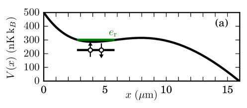
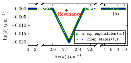
Figure 1: Panel (a): Trap potential, indicating the position of s.p. and two-body resonance states. Panel (b): Complex-momentum contour and Berggren basis states, highlighting the position of the s.p. resonance pole.

We recently introduced the rigged Hilbert space approach to the study of such open quantum systems [8]. This method extends beyond the domain of Hermitian quantum mechanics and includes also time-asymmetric processes such as decays (see e.g. Ref. [9] and references therein). In nuclear physics this formulation has been employed in the Gamow Shell Model [10; 17; 7; 12; 15; 16] to study threshold states and decay processes. Recently, it has also been used to model near-threshold, bound states of dipolar molecules [4].

2 Method

We will obtain solutions of the many-body Hamiltonian for interacting particles using an expansion of s.p. states in the so-called Berggren basis [1]. This complex-momentum basis includes S-matrix poles (bound and resonant states) as well as non-resonant scattering states. The use of this basis, constituting a rigged Hilbert space, is key to our approach as it allows to consistently include the continuum when finding eigensolutions of the open quantum system. The corresponding completeness relation is a generalization of the Newton completeness relation [13] (defined only for real energy states) and reads

$$\sum_{n}|u_{n}\rangle\langle\tilde{u}_{n}|+\int_{L^{+}}dk|u_{k}\rangle\langle\tilde{u}_{k}|=1,$$ (2)

where $|u_{n}\rangle$ correspond to poles of the S-matrix, and the integral of states along the contour $L^{+}$, extending below the resonance poles in the fourth quadrant of the complex-momentum plane, represents the contribution from the non-resonant scattering continuum [1]. This basis also features a non-conjugated inner product.

Single-particle basis

In order to generate the s.p. Berggren basis to be used in the many-body calculation, we start with a complex-momentum basis

$$\left\langle x\vphantom{k,\Pi}\right|\left.k,\Pi\vphantom{x}\right\rangle=\left\{\begin{array}[]{ll}\sqrt{\frac{2}{\pi}}\sin(kx)&(\Pi=0)\\ \sqrt{\frac{2}{\pi}}\cos(kx)&(\Pi=1)\end{array}\right.$$ (3)

that is equivalent to a combination of left- and right-travelling plane waves. In fact, this set corresponds to the Berggren basis for a s.p. Hamiltonian with $V=0$. In practice, the momentum integral of Eq. (2) is performed using Gauss-Legendre quadrature and the momentum basis states are discretized accordingly.

We will use the short-hand notation $\left|k_{i}\right>$ to denote an eigenstate with complex momentum $k_{i}$ and parity $\Pi_{i}$. The matrix representation

$$h_{ij}=\left\langle k_{i}\vphantom{hk_{j}}\right|h\left|k_{j}\vphantom{k_{i}h}\right\rangle$$ (4)

of the one-body Hamiltonian

$$h(x)=-\hbar^{2}/(2m)d^{2}/dx^{2}+V(x)$$ (5)

is in general not Hermitian and not symmetric. The latter property can be recovered by redefining $\tilde{h}_{ij}=\sqrt{\frac{w_{i}}{w_{j}}}h_{ij}$, where $w_{i,j}$ are the Gauss-Legendre weights. The complex-momentum contour $L^{+}$ is selected such that the s.p. resonance energy, which is one of the eigenvalues, appears above the contour in the fourth quadrant. A specific example is shown in Fig. 1(b), in which the contour $L^{+}$ consists of four segments and is truncated at $k=k_{\mathrm{max}}$. The s.p. resonance eigenstate $|u_{\mathrm{res}}\rangle$ can be described as a Gamow state [5]. Such a state behaves asymptotically as an outgoing wave with a complex-energy $e_{\mathrm{res}}=e_{r}-i\gamma_{r}/2$. The imaginary part of the energy corresponds to the decay width $\gamma_{r}$ and gives the half-life of the s.p. state, $t_{1/2}=\ln{(2)}\hbar/\gamma_{r}$, and the s.p. tunneling rate $\gamma_{1}=\gamma_{r}/\hbar$. The full set of eigenvectors to the s.p. Hamiltonian (5) includes the resonance state, as well as non-resonant scattering states with complex momenta very close to the original contour. Together, these eigenstates correspond to our s.p. basis states $U_{1}\equiv\{|u_{i}\rangle\}$ [12].

Many-body problem

The interaction between fermionic atoms in different hyperfine states is modeled by the zero-range potential $V_{12}(x_{1},x_{2})=g\delta\left(x_{1}-x_{2}\right)$, with $g$ the tunable interaction strength. The fermions will be referred to according to their hyperfine spin state as “spin-up” ($\uparrow$) and “spin-down” ($\downarrow$), thus making an obvious connection with systems of spin 1/2 particles (e.g. electrons or nucleons).

We will consider two particles in the trap, being the simplest example of a many-body system. The Hamiltonian is

$$H(x_{1},x_{2})=\sum_{i=1}^{2}\left[-\frac{\hbar^{2}}{2m}\frac{d^{2}}{dx_{i}^{2}}+V(x_{i})\right]+g\delta(x_{1}-x_{2}).$$ (6)

The two-particle basis $T_{2}$ is then naturally constructed from the s.p. bases for the spin-up and -down fermions as $T_{2}\equiv U_{1}(\uparrow)\otimes U_{1}(\downarrow)$. Note that the spin-dependent $c_{B,\sigma}$-term in the trap potential (1) will, in general, result in different s.p. bases for different spin states. In the following we will not directly compare to experimental results and will therefore restrict ourselves to spin-independent trap potentials with $c_{B,\sigma}=1$. Let us first consider the situation of two non-interacting particles, i.e. $g=0$. In this case, the ground state of the system, $|\Phi^{(0)}\rangle$, corresponds to the two distinguishable fermions both occupying the resonant (quasi-bound) state $|u_{\mathrm{res}}\rangle$. In this configuration, both particles are localized in the trap for a finite amount of time, before tunneling out through the potential barrier.

In order to construct the many-body Hamiltonian matrix we first need to evaluate the interaction matrix elements between Berggren states. Note that the basis functions along the complex contour diverge for $x\rightarrow\infty$. As a consequence, the matrix elements of the two-body interaction are not finite in the Berggren basis. We solve this issue by regularizing the two-body matrix elements between states in $T_{2}$ using an expansion in the harmonic oscillator (HO) basis [7]

$$\left\langle u_{i},u_{j}\vphantom{V_{12}u_{l},u_{m}}\right|V_{12}\left|u_{l},u_{m}\vphantom{u_{i},u_{j}V_{12}}\right\rangle=\sum_{\begin{array}[]{l}n_{\alpha},n_{\beta}\\ n_{\gamma},n_{\delta}\end{array}}^{n_{\mathrm{max}}}\left\langle u_{i}\vphantom{n_{\alpha}}\right|\left.n_{\alpha}\vphantom{u_{i}}\right\rangle\left\langle u_{j}\vphantom{n_{\beta}}\right|\left.n_{\beta}\vphantom{u_{j}}\right\rangle\left\langle u_{l}\vphantom{n_{\gamma}}\right|\left.n_{\gamma}\vphantom{u_{l}}\right\rangle\left\langle u_{m}\vphantom{n_{\delta}}\right|\left.n_{\delta}\vphantom{u_{m}}\right\rangle\left\langle n_{\alpha},n_{\beta}\vphantom{V_{12}n_{\gamma},n_{\delta}}\right|V_{12}\left|n_{\gamma},n_{\delta}\vphantom{n_{\alpha},n_{\beta}V_{12}}\right\rangle,$$ (7)

where the sum runs over all HO states up to some truncation $n_{\mathrm{max}}$. In the end, our Hamiltonian (6) matrix in this rigged Hilbert space will be non-Hermitian, but complex symmetric. The spectrum will include bound, resonant and scattering many-body states.

Diagonalization

We will now turn to the problem of finding the resonance state in the eigenspectrum of the many-body Hamiltonian matrix. While there are several algorithms available for finding extreme eigenvalues of Hermitian matrices, our problem is different. We are searching for many-body resonance solutions, $|\Phi_{\mathrm{res}}\rangle$, that are characterized by outgoing boundary conditions and a complex energy $E_{\mathrm{res}}=E_{r}-i\Gamma_{r}/2$, where $\Gamma_{r}$ is the decay width due to the emission of particles out of the trap. In general, these physical states will correspond to specific complex eigenvalues in the interior part of the eigenvalue spectrum. Such eigenstates can be identified by the property that they will be independent of the particular choice of ${L^{+}}$ as long as the Berggren completeness relation (2) holds, i.e. $k_{\mathrm{max}}$ and the number of discretization points both need to be large enough.

However, there exists a simpler method to distinguish these states from the continuum of many-body scattering solutions. The resonance state is usually the state with the largest overlap (in modulus) with $|\Phi^{(0)}\rangle$, referred to as the pole approximation [10]. With the aim of targeting this state we employ the Davidson algorithm for diagonalization [3; 11]. The Davidson method is very efficient at finding eigenvalues for diagonally dominant matrices. The basic idea of this algorithm is that a search space can be constructed by targeting a certain eigenpair. An approximation $\left(|{\phi}_{k}\rangle,\hat{E}_{k}\right)$ for the desired eigenpair $\left(|{\phi}\rangle,E\right)$ is constructed in a subspace of dimension $k$ that is much smaller than the full dimension. The search space is extended iteratively, as in many other methods, but the Davidson algorithm does not rely on a Krylov subspace. At each iteration, we select the Ritz pair $\left(|{\hat{\phi}_{k}}\rangle,\hat{E}_{k}\right)$ that has the largest overlap with the pole approximation, $|\Phi^{(0)}\rangle$. The search space is then extended in the direction of the residual vector $|{r_{k}}\rangle=H|{\hat{\phi}_{k}}\rangle-\hat{E}_{k}|{\hat{\phi}_{k}}\rangle$. Convergence is achieved when the norm of the residual vector approaches zero. The main computational cost of the method is the matrix-vector multiplication that is required at each iteration. For the problems that we consider here, convergence is usually reached within 10-20 iterations as demonstrated in Fig. 2.

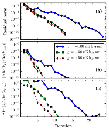
Figure 2: Convergence of the resonance state for three different interaction strengths using the Davidson method. The model space dimension is 57600, corrsponding to $N_{\mathrm{pts}}=240$. Panel (a): Residual norm of the eigenstate. Panel (b): Relative convergence (distance from converged value) of the real part of the eigenvalue. Panel (c): Same as (b) but for the imaginary part of the eigenvalue. The converged eigenvalue is denoted $k_{r,\infty}$.

Many-body tunneling rate

Concerning the tunneling rate we want to stress that there is a priori no simple relation between the decay width and the half life for a many-body system, contrary to the case of a s.p. Gamow state. Assuming exponential decay we would estimate the tunneling rate $\gamma_{\Gamma}=\Gamma_{r}/\hbar=-2\mathrm{Im}(E_{\mathrm{res}})/\hbar$. However, having access to the resonant wave function, $\Phi_{\mathrm{res}}(x_{1},x_{2})\equiv\Phi_{\mathrm{res}}(\mathbf{x})$, we can alternatively compute the decay rate using an integral formalism [6]. The rate of particle emissions can be obtained by integrating the outward flux of particles at large distance ${x_{\mathrm{out}}}$ from the center of the trap, and normalizing by the number of particles on the inside

$$\begin{split}\gamma_{\mathrm{flux}}=\frac{\hbar}{imN({{x_{\mathrm{out}}}})}\sum_{i}\int_{0}^{{x_{\mathrm{out}}}}\prod_{j\neq i}dx_{j}\left[\Phi_{\mathrm{res}}^{*}(\mathbf{x})\frac{d}{dx_{i}}\Phi_{\mathrm{res}}(\mathbf{x})\right.\\ \left.-\left(\frac{d}{dx_{i}}\Phi_{\mathrm{res}}^{*}(\mathbf{x})\right){\Phi_{\mathrm{res}}(\mathbf{x})}\right]_{x_{i}={{x_{\mathrm{out}}}}},\end{split}$$ (8)

with $N({x_{\mathrm{out}}})=\int_{0}^{x_{\mathrm{out}}}\prod_{j}dx_{j}|\Phi_{\mathrm{res}}(\mathbf{x})|^{2}$.

3 Results

In this Contribution we restrict ourselves to the simplest instance of the described tunable open quantum system, the case of two interacting fermions in different spin states in an open 1D potential trap. However, we want to stress that the formalism can be applied to higher-dimensional traps and to systems with more particles. For comparison with experimental results we will use molecular units, in which energy is given in $\mathrm{nK\,k_{B}}$, time in $\mathrm{\mu s}$, and distances in $\mathrm{\mu m}$. In these units we have $\hbar=7638.2\,\mathrm{nK\,k_{B}\,\mu s}$, the Bohr magneton $\mu_{B}=6.7171\cdot 10^{8}\,\mathrm{nK\,k_{B}\,T^{-1}}$ and $\hbar^{2}/m=80.645\,\mathrm{nK\,k_{B}\,\mu m^{2}}$, where $m$ is the mass of a ⁶Li atom.

In Fig. 1(a) we show for illustrative purpose the trap potential with $pV_{0}=2.123\cdot 10^{3}\,\mathrm{nK\,k_{B}}$, $x_{R}=9.975\,\mathrm{\mu m}$, $B^{\prime}=18.90\cdot 10^{-8}\,\mathrm{T\,\mu m^{-1}}$, $c_{B,\sigma}=1$, which closely resemble the parameters extracted from experimental data (see also discussion below). In order to handle the linear term $B^{\prime}x$ we truncate the potential at $x_{\mathrm{cut}}$, sufficiently far away from the relevant trap region. In practice, this is achieved by applying a positive energy shift $E_{\mathrm{shift}}$ so that $V(x_{\mathrm{cut}})+E_{\mathrm{shift}}=0$. The energy shift is subtracted at the end, and we have verified that the fluctuations in the s.p. energy (tunneling rate) with the choice of $E_{\mathrm{shift}}$ was less than $0.04\,\mathrm{\%}$ ($2\,\mathrm{\%}$).

The s.p. Schrödinger equation is solved using the method described above. The discrete set of complex-momentum states $\{\left|k_{i}\right>\}$ that span the contour $L^{+}$ is shown as blue dots in Fig. 1(b). The energy shift that was used is $E_{\mathrm{shift}}=500\,\mathrm{nK\,k_{B}}$. The resulting set of eigenstates (green circles) lies very close to the contour with the exception of one isolated state. The former states correspond to non-resonant scattering solutions, while the latter is a resonance. Together, these eigenstates form the complete set of s.p. basis states, $\{\left|u_{i}\right>\}$, that will be used in the many-body calculation.

The number of points on the contour is increased until convergence of the s.p. resonance energy is achieved. Note that the resonance pole will always remain fixed while the set of scattering states will depend on the choice of the contour $L^{+}$. For illustrative purposes, the contour shown in Fig. 1 consists of only $N_{\mathrm{pts}}=100$ basis states while full calculations were performed with $N_{\mathrm{pts}}=\text{240--320}$. For this set of potential parameters we find $e_{\mathrm{res}}=(301.415-0.08548i)\;\mathrm{nK\,k_{B}}$, which translates into a tunneling rate $\gamma_{1}=22.38\;s^{-1}$.

We now consider the solution of the interacting two-fermion system, projected on the full Berggren basis. We define the interaction energy as

$$E_{\mathrm{int}}\equiv\mathrm{Re}(E_{\mathrm{res}})-2e_{r},$$ (9)

where $\mathrm{Re}(E_{\mathrm{res}})=E_{r}$ is the real part of the resonance energy. Results for the two-particle resonance state as a function of the interaction strength $g$ are shown in Fig. 3.

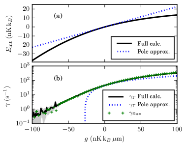
Figure 3: Two-fermion resonance state as a function of the interaction strength $g$ for $c_{B,\sigma}=1$. Panel (a): Interaction energy (9) compared with the corresponding energy obtained using the pole approximation. Panel (b): Tunneling rates obtained from the imaginary part of the resonance energy (from the full calculation and the pole approximation, respectively) compared with the rate obtained from the flux calculation (8).

For $g=0$, the two fermions tunnel out independently and the tunneling rate is equal to $\gamma=2\gamma_{1}=44.76~{}s^{-1}$. However, as the interaction becomes more attractive, the real part of the resonance energy decreases, and the effective barrier seen by the two particles increases. As a consequence the tunneling rate decreases as seen in Fig. 3(b).

Along with the full calculations, we show in Fig. 3 also results obtained in the pole approximation, which corresponds to the single configuration where the two distinguishable fermions occupy the s.p. resonant state. This comparison clearly demonstrates the importance of continuum correlations. The resonance energy and width are both decreased due to configuration mixing between the s.p. resonance pole and non-resonant scattering states. In particular, the energy width, which translates into a decay rate, is very sensitive to these correlations. These results highlight the importance of properly taking the openness of the system into account.

The agreement between the tunneling rate computed from the decay width of the resonance and from the flux formula (8) demonstrates the quality of our numerical approach. It also shows that the tunneling is well approximated by an exponential decay law for this system.

4 Numerical convergence

The stability of the results for the resonance energy, with respect to different model-space parameters, may be investigated in order to assess the numerical precision of the method. We have performed a series of such convergence studies for systems with different interaction strengths ($g=+100,-20,-100\,\mathrm{nK\,k_{B}\,\mu m}$). Panels (a) and (b) of Fig. 4 show the relative change of the resonance energy position for different contours $L^{+}$ and different number of discretization points. Panels (c) and (d) of Fig. 4 demonstrate the convergence with increasing HO truncation in the computation of interaction matrix elements (7). Based on these results we quantify the numerical precision for a specific interaction strength by adding (in quadrature) the amplitudes of variations when the model-space parameters were altered one by one. We found that the precision of the real part of the interaction energy was on the order of $\lesssim 2\,\mathrm{\%}$ for the entire range of interaction strengths. However, the precision of the computed imaginary energy was found to have a lower bound since variations of the computed decay rate was never smaller than 0.5 $s^{-1}$. This becomes obvious when the interaction is strongly attractive and the absolute value of the decay rate is ($\sim$1 $s^{-1}$), see Fig. 4(a).

The larger relative variations in the tunneling rates compared to the interaction energies, as demonstrated in this section, are most likely due to the fact that the imaginary part of the energy is several orders of magnitude smaller than the real part. This means that in order to get precise results for the tunneling rates, an even more precise result for the modulus of the energy is needed. The estimated uncertainties from these numerical studies are shown as shaded bands in both panels of Fig. 3, but is only visible in the tunneling rate for the most attractive interactions ($g\lesssim-60\,\mathrm{nK\,k_{B}\,\mu m}$).

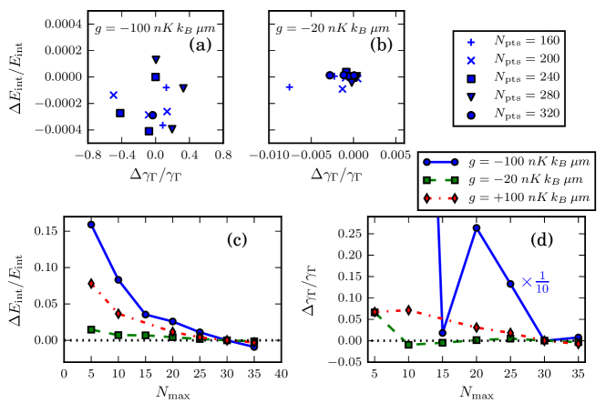
Figure 4: Convergence study for the two-body problem with different interaction strengths. The upper row shows relative changes of the resonance pole position with different contours and different number of dicretization points, for strong attraction (panel a) and intermediate attraction (panel b). The two lower rows show the relative change of the real part (panel c) and imaginary part (panel d) of the resonance energy with increasing HO truncation in the calculation of two-body matrix elements (7).

5 Concluding remarks

The tunneling of few fermions from low-dimensional traps were measured by Zürn et al [20]. The analysis of data from this experiment is quite complicated and involves the use of the WKB approximation to extract the trap potential parameters. More precisely, $pV_{0}$ and $B^{\prime}$ in Eq. (1) were adjusted such that the s.p. tunneling rates obtained in the WKB approximation matched the experimental results. We studied this experiment in a recent publication [8] using the method outlined in this Contribution. Using the set of parameters given in Ref. [20] as input to our exact diagonalization approach we found a good agreement for the s.p. energies (with a difference of at most a few percent), while s.p. tunneling rates were almost two times larger than the ones published in Ref. [20]. The main conclusion from these findings is that that the WKB method should not be expected to produce reliable estimates for the tunneling rate and that the analysis of experimental results for open quantum systems is highly sensitive to the determination of trap parameters.