Random matrix ensembles involving Gaussian Wigner and Wishart matrices,
and biorthogonal structure
Abstract
We consider four nontrivial ensembles involving Gaussian Wigner and Wishart matrices. These are relevant to problems ranging from multiantenna communication to random supergravity. We derive the matrix probability density, as well as the eigenvalue densities for these ensembles. In all cases the joint eigenvalue density exhibits a biorthogonal structure. A determinantal representation, based on a generalization of Andréief’s integration formula, is used to compactly express the -point correlation function of eigenvalues. This representation circumvents the complications encountered in the usual approaches, and the answer is obtained immediately by examining the joint density of eigenvalues. We validate our analytical results using Monte Carlo simulations.
pacs:
05.45.-a, 02.10.Yn, 02.50.Sk, 89.70.-aI Introduction
Wigner and Wishart matrices have been the cornerstones of random matrix theory. They find numerous applications in varied fields of knowledge Mehta2004 ; Forrester2010 ; Handbook2011 . The inception of Wigner matrices was due to Wigner who investigated some special large dimensional random matrices to predict properties of the eigenfunctions and eigenvalues of complicated quantum mechanical systems, in particular heavy nuclei Wigner1955a ; Wigner1958 . It turns out that certain spectral characteristics of these matrices, such as semicircular distribution of eigenvalues, are universal and in fact shared by a wider class of matrices which are now collectively referred to as Wigner matrices. See, for example, Refs. Erdos2011 ; TV2012 for recent surveys. An important family of Wigner matrices is realized when the matrix elements are taken as Gaussian random variables. The resulting ensembles are referred to as Gaussian ensembles Mehta2004 ; Forrester2010 ; Dyson1972 . In the present work we use the terms Wigner and Gaussian Wigner interchangeably to mean complex Wigner matrices with Gaussian entries, more specifically matrices from the Gaussian unitary ensemble Mehta2004 ; Forrester2010 ; Dyson1972 . Wishart matrices predate even Wigner matrices and have their origin in the field of multivariate statistics. These were introduced by Wishart who derived the generalized product-moment distribution in normal multivariate population samples Wishart1928 . This distribution is now referred to as the Wishart distribution. In what follows, we will be concerned with ensembles comprising complex Wishart matrices.
While Wigner and Wishart matrices themselves offer plenty of aspects to explore, interestingly, various combinations of these also turn out to be of crucial importance. Many such matrix ensembles have their origin in the area of multivariate statistics GN1999 ; Anderson2003 ; Muirhead2005 . A classic example is the Jacobi (MANOVA) ensemble which incorporates two Wishart matrices in a nontrivial manner, and arises in the problems of quantum conductance SM2006 ; Forrester2006 ; SSW2008 ; KSS2009 ; KP2010a ; KP2010b and multiple channel fiber optics communication DFS2013 ; KMV2014 . Remarkably, it also pops up in something as remote as a microscopic model of bus transport system BBDS2006 . In recent years several other important matrix models have been explored. Some notable examples include product of complex Ginibre matrices AIK2013 ; AKW2013 ; KZ2014 ; WZCT2014 ; AI2015 ; ZWSMHC2015 ; Kieburg2015 , Cauchy-Lorentz Kieburg2015 ; Brouwer1995 ; BJJNPZ2002 ; MMSV2014 ; KKG2014 ; WWKK2015 , sum involving Wigner and Wishart matrices MMW2012 ; PW2014 ; LMM2014 ; Kumar2014 ; KGGC2015 ; CKW2015 , and product of truncated unitary matrices ABKN2014 . In addition to their natural connection with multivariate statistics, these are of interest to the fields of telecommunication AIK2013 ; KGGC2015 ; ZWSMHC2015 , finance BJNPZ2003 ; BJNPZ2004 , and random supergravity theory MMW2012 ; PW2014 ; LMM2014 .
In the present work we proceed further in exploring such exotic ensembles and consider four important matrix models involving Wigner and Wishart matrices. The first one comprises a ratio involving two Wishart matrices, the second one consists of the weighted sum of a Wigner matrix and a Wishart matrix, the third is the product of a Wigner matrix and a Wishart matrix, and the fourth one embodies the weighted sum of two Wishart matrices. We derive the probability density function for these matrices, and then work out the eigenvalue statistics. The joint density of eigenvalues for these matrix models exhibit biorthogonal structure. A determinantal representation, based on a generalization of Andréief’s integration formula Andreief1883 ; KG2010a ; KG2010b , is used to compactly express the -point correlation function for all these ensembles.
The rest of the paper is organized as follows. We start with a brief discussion of biorthogonal ensembles in Sec. II, and present the result for -level correlation function for eigenvalues. Sections III–VI are devoted to the exact results for the above mentioned matrix ensembles which involve nontrivial combinations of Wigner and Wishart matrices. We conclude in Sec. VII with a brief summary and outlook. Some relevant derivations are presented in the Appendices.
II Biorthogonal ensembles
Biorthogonal ensembles arise naturally in the study of eigenvalue statistics of two matrix models BE2006 ; Bertola2007 . Moreover, matrix ensembles with a unitary invariance breaking external source also give rise to biorthogonal structure BK2004 ; BH1996 ; BH1998 . These ensembles exhibit rich mathematical structure and, at the same time, find applications in several important problems which range from quantum transport to multiple antenna telecommunication, to two-dimensional gravity Muttalin1995 ; Frahm1995 ; Borodin1998 ; DF2008 ; ZCW2009 ; AIK2013 ; AKW2013 ; KZ2014 ; WZCT2014 ; Zhang2015 ; DKK1993 .
We are interested here in biorthogonal ensembles of the Borodin type Borodin1998 , which possess the following structure for joint density of its eigenvalues ():
| (1) |
Here is a well-behaved weight function in the desired domain, and represents determinant. Also, is the Vandermonde determinant,
| (2) |
The normalization factor follows by expanding the determinants and performing the integrals. The ensuing expression can again be represented as a determinant, as asserted by Andréief identity Andreief1883 . We have
| (3) |
where
| (4) |
For the special case of , we obtain the joint probability density of eigenvalues for a unitary random matrix ensemble. We note that if we replace by some other determinant , then we have the most general form of biorthogonal ensemble, as defined by Borodin Borodin1998 . The approach for calculating correlation function, as discussed below, extends to these as well.
We would like to remark that the biorthogonal ensemble of Borodin type emerges after integrating out one set of eigenvalues (corresponding to one of the matrices) from the joint probability density of eigenvalues for two-matrix model; see for example Appendix B.
The -point correlation function corresponding to Eq. (1) is defined as Mehta2004
| (5) |
The evaluation of this correlation function usually relies on the explicit construction of biorthogonal polynomials. In Borodin1998 a recipe has been provided to write down the correlation function in terms of a determinant of a -dimensional matrix with entries containing certain two-point kernel. However, it requires inversion of a matrix.
In the following we use a generalization of Andréief’s integration formula to express the -point correlation function in terms of the determinant of an -dimensional matrix KG2010a ; KG2010b :
| (6) |
In the above expression represents block with all entries 0, and are as appearing in Eqs. (1) and (4), respectively. In Appendix A we provide a proof of Eq. (II) based on mathematical induction. The above representation for correlation function altogether circumvents the complications encountered in the approaches described above, and an explicit answer is obtained at once. For small Eq. (II) is advantageous in the sense that it can be readily implemented and evaluated in computational packages such as Mathematica Mathematica . In particular the first-order marginal density of eigenvalues, which is related to the one-point correlation function as , is given by
| (7) |
A similar form has been used in RKGZ2012 ; Kumar2014 to express the marginal density of eigenvalues. On the other extreme, if we consider , then the determinant in Eq. (II) collapses to the product of determinants and , along with the factor , and thereby yields , as expected.
As discussed in the Introduction, in the following sections we consider four matrix ensembles where such biorthogonal structure emerges. The joint density of eigenvalues for these ensembles appear in the form of Eq. (1), and hence the -point correlation function can be written down immediately with the aid of Eq. (II).
III Ratio involving two Wisharts
III.1 Matrix model and probability density
We consider an ensemble of dimensional complex matrices
| (8) |
where and are some non-negative scalars (for definiteness), and and are positive-definite Hermitian matrices, respectively, from the complex Wishart distributions
| (9) |
Here are the respective degrees of freedom for the two distributions. We may refer to the ensemble described by Eq. (8) as a quotient ensemble. For we have the usual complex Wishart, while the limit leads to the ensemble , which is a multivariate generalization of the beta distribution of the second kind Kumar2015 . We also note that , and share the identical nonnegative eigenvalues as they correspond to the same generalized eigenvalue problem and lead to the secular equation . We will see below that the above construction leads to a very interesting matrix model whose probability density involves confluent hypergeometric function of the second kind (Tricomi’s function) with matrix argument JJ1985 . Moreover, this matrix model is of direct relevance to the problem of multiple antenna relay systems TV2005 .
The probability density of can be calculated as
| (10) |
Here the delta function with matrix argument represents the product of delta functions with scalar arguments, one for each independent real and imaginary component of . Also, , etc. represent the flat measure involving the product of the differentials of all independent variables occurring within the matrix. Implementation of the Fourier representation for delta function and the cyclic invariance property of trace gives
| (11) |
The matrix in the above equation possesses symmetry properties identical to those of . Using Eq. (9), reordering the integrals, and considering the transformation , we obtain
| (12) |
Integration over yields
| (13) |
The integral can be identified as a variant of Ingham-Siegel-Fyodorov integral F2002 and leads to
| (14) |
We may write
| (15) |
where
| (16) |
can be expressed in terms of the confluent hypergeometric function of the second kind (Tricomi’s function) with matrix argument JJ1985 ,
| (17) |
as
| (18) |
Here is the multivariate Gamma function:
| (19) |
Thus, we finally have the result
| (20) |
III.2 Eigenvalue statistics
We now derive the joint density of eigenvalues for the matrix model of Eq. (8). As implied by the result in Appendix B, of Eq. (17) admits the following determinantal representation in terms of elements involving hypergeometric function of the second kind (Tricomi’s function) with scalar argument BE1953 ; AS1972 :
| (21) |
Here ’s are the eigenvalues of . The joint density of eigenvalues () of , therefore, follows immediately from Eq. (III.1), and possesses the biorthogonal structure as in Eq. (1) with
| (22) |
| (23) |
The of Eq. (4) is obtained as
| (24) |
We used here the integral result
| (25) |
which holds whenever the integral is convergent. Therefore, -point correlation function and the marginal density follow immediately from Eqs. (II) and (7).
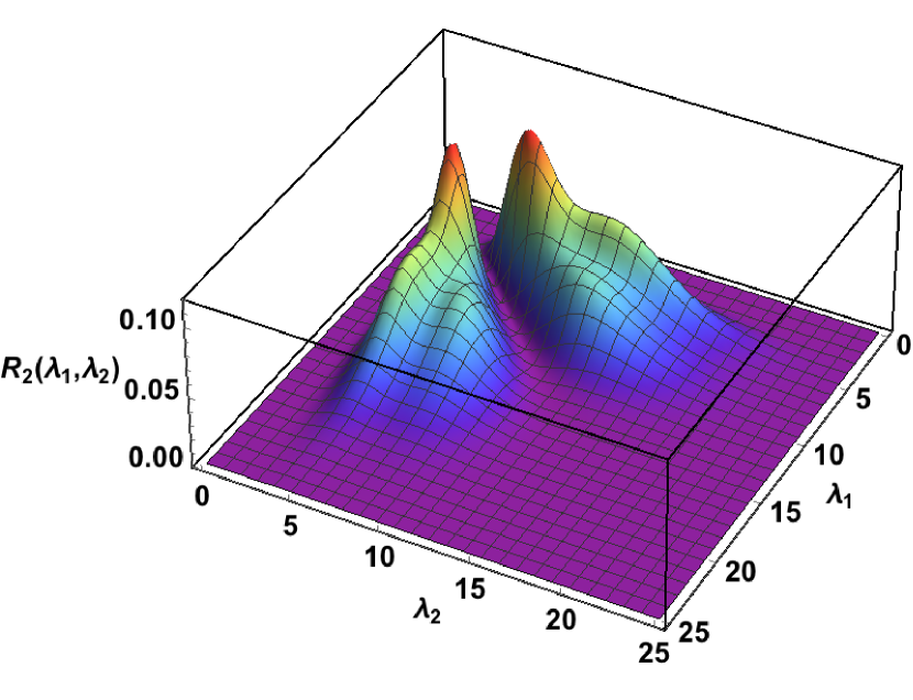
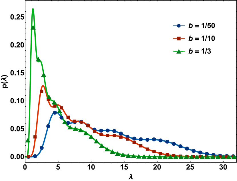
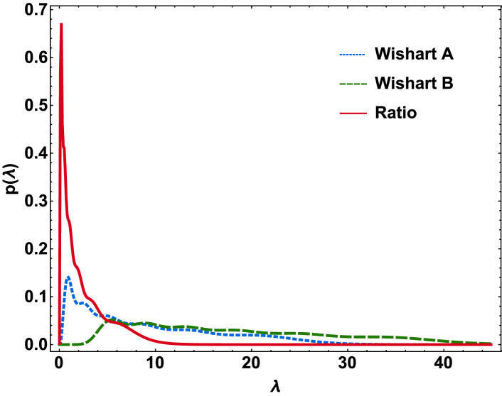
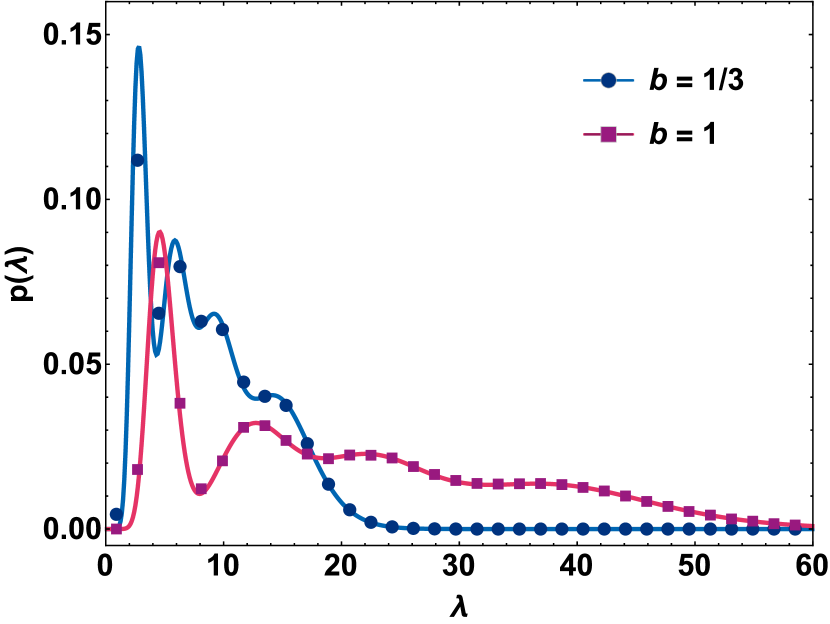
In Fig. 1(a) we show the two-point correlation function for parameter values indicated in the caption. Although not shown here for the sake of clarity, a two-dimensional histogram obtained using Monte-Carlo simulation agrees well with the analytical plot. In Fig. 1(b) marginal density of eigenvalues is shown for parameter values mentioned in the caption. In this case simulation results are also depicted with the aid of symbols, and are in excellent agreement with the analytical curves. As already indicated, the parameters and give freedom to realize a variety of densities using two Wishart matrices, the exact outcome being dependent on the dimensions of the constituent matrices. As an example, in Fig. 2 we show the density corresponding to the quotient ensemble defined by Eq. (8) along with the densities of the constituent Wishart matrices, which can be calculated using the result
| (26) |
Here represents associated Laguerre polynomial of degree , and the parameter is given by or , i.e., it is the difference of degree of freedom and dimension of the Wishart matrix. We should underline that the resulting spectra, tunable by and , can have a crucial role in deciding the behavior of metric which follow from the eigenvalue statistics, such as channel capacity and outage probability in the case of multiple access channel (MAC) and interference channel (IC) in multiple-input multiple-output (MIMO) communication TV2005 .
IV Weighted sum of a Wigner and a Wishart
IV.1 Matrix model and probability density
We now consider an ensemble comprising weighted sum of Wigner and Wishart matrices:
| (27) |
Here and are respectively -dimensional Hermitian and positive-definite-Hermitian matrices from the distributions
| (28) |
and , as before, are non-negative scalars. Also, . For , with , we have the Wigner (Gaussian unitary) ensemble. On the other hand, for , with , we obtain the Wishart (Laguerre unitary) ensemble. Therefore, by considering , and by varying between 0 and 1, we have an ensemble which interpolates between the Wishart and Wigner ensembles. To the best of our knowledge, for this matrix model only the first order marginal density of eigenvalues is known in the large asymptotic regime using the tools of free probability Speicher1993 . A matrix ensemble similar to that in Eq. (27) has been used to model the Hessian matrix in the context of supergravity MMW2012 ; PW2014 ; LMM2014 .
To obtain the probability density function for we introduce the Fourier representation of delta function as in Eq. (III.1). Reordering of the integrals, and use of the cyclic invariance property of trace then gives
| (29) |
Evaluation of the Gaussian integral involving leads to
| (30) |
The Gaussian integral over can also be performed and yields
| (31) |
where
| (32) |
IV.2 Eigenvalue statistics
We now calculate the eigenvalue statistics corresponding to Eq. (31). Using the result in Appendix B we know that is determined solely by the eigenvalues () of as
| (33) |
where
| (34) |
This integral can be evaluated in terms of confluent hypergeometric function of the first kind (Kummer’s function) BE1953 ; AS1972 , and leads to the joint density, Eq. (1), with 111For , a much simpler representation is possible in terms of confluent hypergeometric function of the second kind.
| (35) |
The weight function is read from Eq. (31) as
| (36) |
In this case obtaining a closed form for requires some effort. A possible representation is in terms of hypergeometric BE1953 ; AS1972 :
| (37) |
With the above explicit results, the -point correlation function of Eq. (II) is readily obtained.
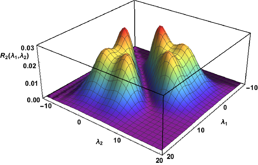
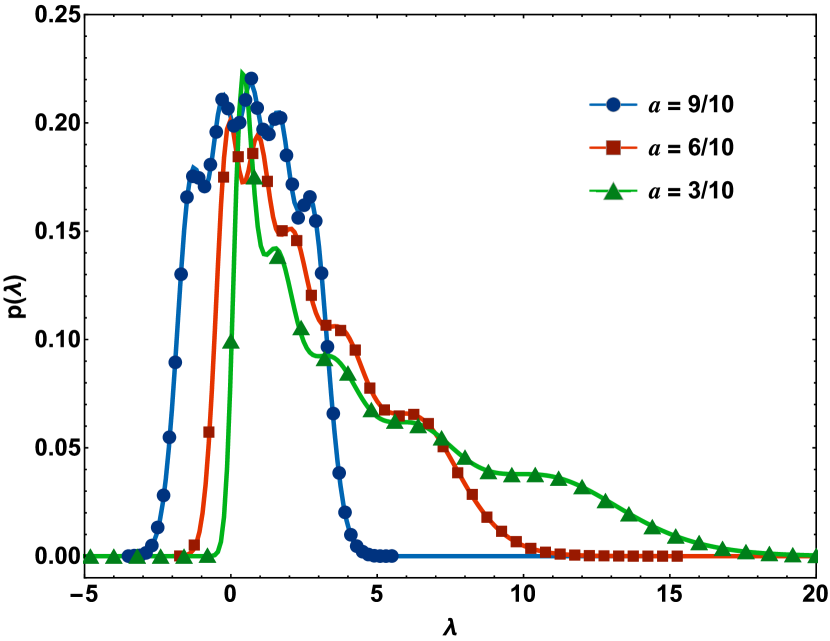
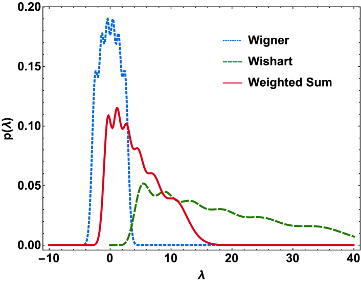
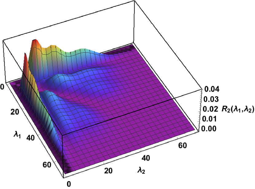
We show the two-point correlation function surface in Fig. 3(a). The marginal density is shown along with the Monte-Carlo simulation outcome in Fig. 3(b). In particular, for Fig. 3(b) we have considered . Therefore, a crossover is seen from Wigner density (semicircle type) to Wishart density (Marčenko-Pastur type). In Fig. 4 we compare the eigenvalue density of the composite ensemble with the eigenvalue density for the constituent Wishart ensemble given by Eq. (III.2) and that of the Gaussian Wigner ensemble evaluated using
| (38) |
Here represents the Hermite polynomial of degree . We can see that the Wishart constituent of the composite matrix tends to keep the eigenvalues in the positive half of the real line, while the Wigner part pulls them toward the negative half and tries to make the density symmetric about zero, thereby giving rise to an interesting hybrid density.
V Product of a Wigner and a Wishart
V.1 Matrix model and probability density
We now consider an ensemble defined by
| (39) |
where and , respectively, are Wigner and Wishart matrices from the distributions given in (28). We note here that is Hermitian but is Hermitian and positive-definite as well; therefore, the signs of eigenvalues of are decided by the respective signs of eigenvalues of Serre2010 . As a consequence we expect the resultant first order marginal density to be symmetric about the origin, similar to that in the Wigner case.
We introduce the matrix delta function, as in Eq. (III.1), to obtain
| (40) |
We reorder the integrals and use the cyclic invariance of trace to get
| (41) |
Integral over can be done to give
| (42) |
We now employ the transformation , which leads to
| (43) |
The -integral can now be performed F2002 and yields
| (44) |
with
| (45) |
Here represents the Heaviside theta function and requires to be positive-definite for a non-vanishing result.
V.2 Eigenvalue statistics
With a little modification the result in Appendix B implies that is determined by the eigenvalues () of as
| (46) |
where
| (47) |
with for and for . This integral can be evaluated compactly in terms of Meijer G-function BE1953 as
| (50) |
Meijer G-functions have also appeared in the correlation kernels for product of complex Ginibre matrices AIK2013 ; AKW2013 ; KZ2014 ; WZCT2014 ; AI2015 ; ZWSMHC2015 ; Kieburg2015 , and product of truncated unitary matrices ABKN2014 . The weight function , in view of Eq. (44), is
| (51) |
which leads to the following expression of :
| (52) |
Equation (II) now determines correlation functions of all orders for the matrix model (39).
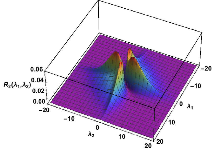
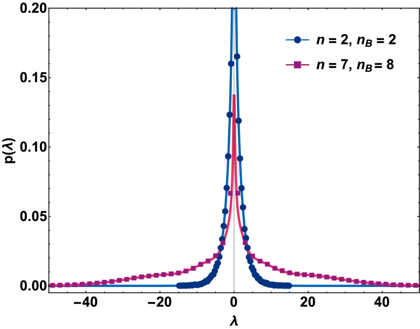
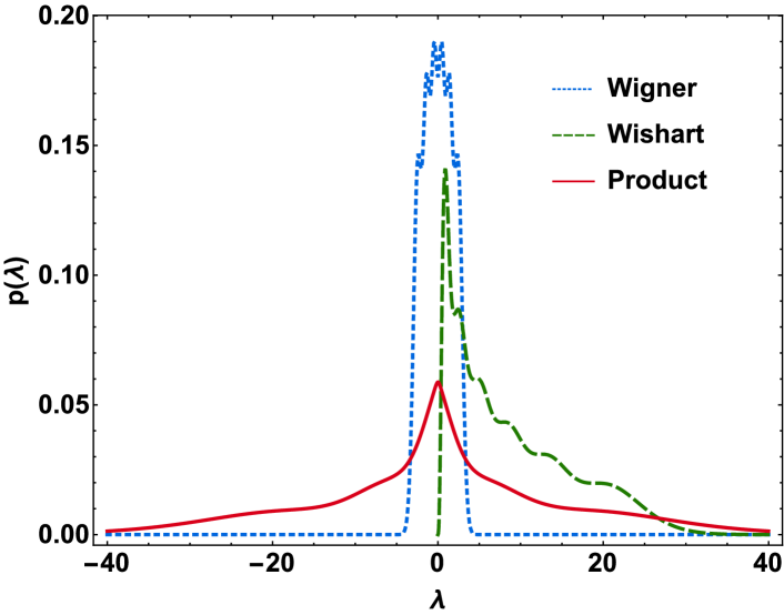
Figure 5(a) shows the two-point correlation function of eigenvalues, while Fig. 5(b) depicts the marginal density. For the density exhibits a logarithmic singularity at . This can be seen in plot in Fig. 5(b). In Fig. 6 we display the eigenvalue density for the product of Wigner and Wishart matrices, along with the densities for the constituent matrices calculated using Eqs. (III.2) and (38). Figure 6 should be compared with Fig. 4 where we have used matrices with dimensions same as in the present case. The distinct nature of the resultant densities in these two cases is expected because of very different characteristics of the underlying composition. The shapes of the marginal density curves here are reminiscent of the density of eigenvalues of adjacency matrices in scale free networks JB2007 ; BJ2007 ; NR2008 and matrices defined on Poissonian random graphs Kuhn2008 .
VI Weighted sum of two Wisharts
VI.1 Matrix model and probability density
We finally consider the matrix model
| (53) |
where and are -dimensional positive-definite-Hermitian matrices, respectively, from the distributions
| (54) |
with . The parameters are again non-negative scalars. We have taken the covariance matrix equal to identity matrix for , while for we have assumed an arbitrary (positive definite) covariance matrix. The latter constitutes the correlated variant of the Wishart ensemble. The above matrix model has been considered in Kumar2014 and exact results have been obtained for the matrix probability density, the joint probability density of eigenvalues, as well as the first order marginal density.
We would like to remark that if one considers covariance matrices proportional to identity matrix only, then the problem can be solved for the weighted sum of arbitrary number of Wishart matrices. Such a scenario has been considered in KGGC2015 and the results used for the analysis of multiuser communication employing multiantenna elements such as multiple-input multiple-output (MIMO) multiple access channel (MAC).
For the matrix model of Eq. (53), with parameter , the probability density function satisfied by matrix reads Kumar2014
| (55) |
where is confluent hypergeometric function of the first kind (Kummer’s function) with matrix argument:
| (56) |
Here is the multivariate beta function:
| (57) |
Similar to the beta function with scalar arguments, it is related to multivariate gamma function in Eq. (19) as
| (58) |
VI.2 Eigenvalue statistics
The joint probability density of eigenvalues () for Eq. (53) is given by Eq. (1) with
| (59) |
| (60) |
where are the eigenvalues of Kumar2014 . Also, can be obtained using the result
| (61) |
valid for convergent scenarios, as
| (62) |
Consequently, we obtain an explicit result for the -point correlation function.
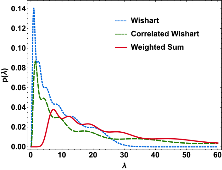
Figure 7(a) shows the two-point correlation function of eigenvalues for matrix model given in Eq. (53), while Fig. 7(b) depicts the marginal density. In Fig. 8 we compare the densities of Wishart, correlated-Wishart and their weighted sum. For density of the correlated-Wishart we have used the following result, which also follows with the aid of Eq. (7):
| (63) |
where . We note that while matrix models (8) and (53) can lead to similar densities in particular scenarios (e.g. when ), in general they exhibit different behavior. For instance, the present model can not lead to the multivariate-beta-distribution kind of density which can be achieved using Eq. (8) for .
VII Conclusion and Outlook
We considered four important matrix models which lead to biorthogonal structure in their joint eigenvalue densities. These matrix ensembles play important roles in several areas, which range from multiple antenna communication theory to supergravity theory. We evaluated the matrix distribution, as well as the joint eigenvalue density for these ensembles. With the information of joint density, we also presented determinantal expression for eigenvalue correlation function of arbitrary order. This representation follows from a generalization of Andréief’s integration formula. Since knowledge of the correlation function gives access to the prediction of statistical behavior of observables of interest in a given problem, we believe that the exact results derived here will find interesting applications in several fields.
As continuation of the present work, an immediate direction to pursue could be the investigation of the behavior of extreme eigenvalues of the composite matrix models, and its comparison with that of the extreme eigenvalues of the constituent matrices. This will give a better insight into the mechanism by which the redistribution of eigenvalues takes place. Since all the matrix models considered here possess biorthogonal structure in their joint eigenvalue density expressions, exact results are possible for the gap probabilities and densities of extreme eigenvalues Kumar2015 .
While we considered here ensembles comprising complex matrices, the cases of real and quaternion matrices are also important and can be explored. However, solving these ensembles poses serious challenges because of unavailability of group integral results similar to those in the case of unitary group. Another interesting direction can be the analysis of the spectra of the composite matrices in large dimension limit, and to look for universalities.
Appendix A Correlation function
We will use mathematical induction to prove Eq. (II). Equations (5) and (II) are defined for 222 One may define being equal to 1.. From the definition of correlation function, Eq. (5), it is clear that
| (64) |
For Eq. (II) clearly holds, since in this case the determinant in Eq. (II) factorizes into the product of two determinants and produces . Let us assume it is correct for . We will prove that given this, Eq. (II) holds for as well. Using Eq. (64) we obtain
| (65) |
We expand the determinant using the ’th row:
| (66) |
We now insert the in the ’th column, and perform the integral. Using the definition of given in Eq. (4) , we obtain
| (67) |
Performing separate row interchanges in the determinants appearing in the sum, we arrive at
| (68) |
where is the Kronecker-delta function. Using multilinearity property in first rows in determinant appearing in each of the terms in the above summation, we find that it gives rise to
| (69) |
Plugging this back in Eq. (65), we obtain an expression for which is consistent with Eq. (II), and hence the desired result follows.
Appendix B Matrix Integral
Consider -dimensional Hermitian matrices and . We are interested in evaluating integral of the form
| (70) |
where is a scalar and is a unitarily invariant expression involving , such that the above integral is convergent. We note that Eq. (70) is a matrix generalization of Laplace transform. If and are the diagonal matrices consisting of eigenvalues of and , then
| (71) |
where represents the Haar measure over the group of -dimensional unitary matrices. The unitary group integral can be performed using the celebrated Harish-Chandra–Itzykson-Zuber formula HC1956 ; IZ1980 and leads to
| (72) |
Now if is expressible in terms of certain weight functions as , then integral over can be performed and results in
| (73) |
where
| (74) |
Note that we may consider (or/and ) for within the determinant in (1) and then accordingly modify the rest of the results in Sec. II which depend on .
References
- (1) M. L. Mehta, Random Matrices (Academic Press, New York, 2004).
- (2) P. J. Forrester, Log-Gases and Random Matrices (LMS-34) (Princeton University Press, Princeton, NJ, 2010).
- (3) Handbook of Random Matrix Theory, edited by G. Akemann, J. Baik, and P. Di Francesco (Oxford Press, New York, 2011).
- (4) E. P. Wigner, Ann. Math. 62, 548 (1955); 65, 203 (1957).
- (5) E. P. Wigner, Ann. Math. 67, 325 (1958).
- (6) L. Erdős, Russ. Math. Surv. 66, 507 (2011).
- (7) T. Tao and V. Vu, in Proceedings of Symposia in Applied Mathematics, Vol. 72, edited by Van H. Vu (Yale University, New Haven, CT, 2014), p. 121.
- (8) F. J. Dyson, J. Math. Phys. 13, 90 (1972).
- (9) J. Wishart, Biometrika A 20, 32 (1928).
- (10) A. K. Gupta and D. K. Nagar, Matrix Variate Distributions, (CRC Press, Boca Raton, FL, 1999), Vol. 104 .
- (11) T. W. Anderson, An Introduction to Multivariate Statistical Analysis, 3rd ed. (John Wiley & Sons, New York, 2003).
- (12) R. J. Muirhead, Aspects of Multivariate Statistical Theory (Wiley Interscience, New York, 2005).
- (13) S. H. Simon and A. L. Moustakas, Phys. Rev. Lett. 96, 136805 (2006).
- (14) P. J. Forrester, J. Phys. A: Math. Gen. 39, 6861 (2006).
- (15) D. V. Savin, H.-J. Sommers, and W. Wieczorek, Phys. Rev. B 77, 125332 (2008).
- (16) B. A. Khoruzhenko, D. V. Savin, and H.-J. Sommers, Phys. Rev. B 80, 125301 (2009).
- (17) S. Kumar and A. Pandey, J. Phys. A: Math. Theor. 43, 085001 (2010).
- (18) S. Kumar and A. Pandey, J. Phys. A: Math. Theor. 43, 285101 (2010).
- (19) R. Dar, M. Feder, and M. Shtaif, IEEE Trans. Inf. Theor. 59, 2426 (2013).
- (20) A. Karadimitrakis, A. L. Moustakas, and P. Vivo, IEEE Trans. Inf. Theor. 60, 4370 (2014).
- (21) J. Baik, A. Borodin, P. Deift, and T. Suidan, J. Phys. A: Math. Gen. 39, 8965 (2006).
- (22) G. Akemann, J. R. Ipsen, and M. Kieburg, Phys. Rev. E 88, 052118 (2013).
- (23) G. Akemann, M. Kieburg, and L. Wei, J. Phys. A: Math. Theor. 46, 275205 (2013).
- (24) A. B. J. Kuijlaars and L. Zhang, Commun. Math. Phys. 332, 759 (2014).
- (25) L. Wei, Z. Zheng, J. Corander, and G. Taricco, IEEE Trans. Commun. 63, 1700 (2015).
- (26) Z. Zheng, L. Wei, R. Speicher, R. Müller, J. Hämäläinen, and J. Corander, arXiv:1502.05516.
- (27) G. Akemann and J. R. Ispen, arXiv:1502.01667.
- (28) M. Kieburg, arXiv:1502.00550.
- (29) P. W. Brouwer, Phys. Rev. B 51 16878 (1995).
- (30) Z. Burda, R. A. Janik, J. Jurkiewicz, M. A. Nowak, G. Papp, and I. Zahed, Phys. Rev. E 65, 021106 (2002).
- (31) R. Marino, S. N. Majumdar, G. Schehr, and P. Vivo, J. Phys. A: Math. Theor. 47, 055001 (2014).
- (32) V. Kaymak, M. Kieburg and T. Guhr, J. Phys. A: Math. Theor. 47, 295201 (2014).
- (33) T. Wirtz, D. Waltner, M. Kieburg, and S. Kumar, arXiv:1505.00675.
- (34) D. Marsh, L. McAllister, and T. Wrase, J. High Energy Phys. 1203,102 (2012).
- (35) F. G. Pedro and A. Westphal, Phys. Lett. B 739 439 (2014).
- (36) C. Long, L. McAllister, and P. McGuirk, J. High Energy Phys. 10, 187 (2014).
- (37) S. Kumar, Europhys. Lett. 107, 60002 (2014).
- (38) S. Kumar, G. F. Pivaro, G. Fraidenraich, and C. F. Dias, arXiv:1504.00222.
- (39) T. Claeys, A. B. J. Kuijlaars, and D. Wang, arXiv:1505.00610.
- (40) G. Akemann, Z. Burda, M. Kieburg, and Taro Nagao, J. Phys. A: Math. Theor. 47, 255202 (2014).
- (41) Z. Burda, J. Jurkiewicz, M. A. Nowak, G. Papp, and I. Zahed, Acta Phys. Pol. B 34, 4747 (2003).
- (42) Z. Burda, J. Jurkiewicz, M. A. Nowak, G. Papp, and I. Zahed, Physica A 343, 694 (2004).
- (43) C. Andréief, Mém. de la Soc. Sci. Bordeaux 2, 1 (1883).
- (44) M. Kieburg and T. Guhr, J. Phys. A: Math. Theor. 43, 075201 (2010).
- (45) M. Kieburg and T. Guhr, J. Phys. A: Math. Theor. 43, 135204 (2010).
- (46) M. Bertola and B. Eynard, Math. Phys. Anal. Geom. 9, 23 (2006).
- (47) M. Bertola, J. Approx. Theor. 144, 162 (2007).
- (48) P. M. Bleher and A. B. J. Kuijlaars, Commun. Math. Phys. 252, 43 (2004).
- (49) E. Brézin and S. Hikami, Nucl. Phys. B 479, 697 (1996).
- (50) E. Brézin and S. Hikami, Phys. Rev. E 58, 7176 (1998).
- (51) J.-M. Daul, V. A. Kazakov, and I. K. Kostov, Nucl. Phys. B 409, 311 (1993).
- (52) K. A. Muttalib, J. Phys. A: Math. Gen. 28, L159 (1995).
- (53) K. Frahm, Phys. Rev. Lett. 74, 4706 (1995).
- (54) A. Borodin, Nucl. Phys. B 536, 704 (1998).
- (55) P. Desrosiers and P. J. Forrester, J. Approx. Theor. 152, 167 (2008).
- (56) A. Zanella, M. Chiani, and M. Z. Win, IEEE Trans. Commun. 57, 1050 (2009).
- (57) L. Zhang, J. Stat. Phys. (to be published), arXiv:1502.03160
- (58) Wolfram Research Inc., Mathematica Version 10.0, Champaign, IL, 2014.
- (59) C. Recher, M. Kieburg, T. Guhr, and M. R. Zirnbauer, J. Stat. Phys. 148, 981 (2012).
- (60) S. Kumar, arXiv:1507.08830
- (61) R. M. Joshi and J. M. C. Johsi, Indian J. Pure Appl. Math. 16 627 (1985).
- (62) D. Tse and P. Viswanath, Fundamentals of Wireless Communication (Cambridge University Press, Cambridge, UK, 2005).
- (63) Y. V. Fyodorov, Nucl. Phys. B 621, 643 (2002).
- (64) H. Bateman and A. Erdélyi, Higher Transcendental Functions, Vol. I (McGraw-Hill, New York, 1953).
- (65) Handbook of Mathematical Functions with Formulas, Graphs, and Mathematical Tables, edited by M. Abramowitz and I. A. Stegun (Dover, New York, 1972).
- (66) R. Speicher, Publ. RIMS Kyoto Univ. 29, 731 (1993).
- (67) D. Serre, Matrices: Theory and Applications, 2nd ed. (Springer, New York, 2010), p. 109.
- (68) J. N. Bandyopadhyay and S. Jalan, Phys. Rev. E 76, 026109 (2007).
- (69) S. Jalan and J. N. Bandyopadhyay, Phys. Rev. E 76, 046107 (2007).
- (70) T. Nagao and G. J. Rodgers, J. Phys. A: Math. Theor. 41, 265002 (2008).
- (71) R. Kühn, J. Phys. A: Math. Theor 41, 295002 (2008).
- (72) Harish-Chandra, Amer. J. Math. 79, 87 (1957).
- (73) C. Itzykson and J.-B. Zuber, J. Math. Phys. 21, 411 (1980).