Modal Analysis Using Sparse and Co-prime Arrays

Pooria Pakrooh,  Louis L. Scharf, , and Ali Pezeshki,  This work is supported in part by NSF under grants CCF-1018472 and CCF-1422658.A preliminary version of a subset of the results reported here was presented at the 2014 Asilomar Conference on Signals, Systems, and Computers, Pacific Grove, CA, Nov. 2-5, 2014, in a paper entitled “Characterization of orthogonal subspaces for alias-free reconstruction of damped complex exponential modes in sparse arrays,” by P. Pakrooh, A. Pezeshki, and L. L. Scharf.P. Pakrooh is with the Department of Electrical and Computer Engineering, Colorado State University, Fort Collins, CO 80523, USA (e-mail: Pooria.Pakrooh@colostate.edu).L. L. Scharf is with the Department of Mathematics and the Department of Statistics, Colorado State University, Fort Collins, CO 80523, USA (e-mail: Louis.Scharf@colostate.edu).A. Pezeshki is with the Department of Electrical and Computer Engineering and the Department of Mathematics, Colorado State University, Fort Collins, CO 80523, USA (e-mail: Ali.Pezeshki@colostate.edu).
Abstract

Let a measurement consist of a linear combination of damped complex exponential modes, plus noise. The problem is to estimate the parameters of these modes, as in line spectrum estimation, vibration analysis, speech processing, system identification, and direction of arrival estimation. Our results differ from standard results of modal analysis to the extent that we consider sparse and co-prime samplings in space, or equivalently sparse and co-prime samplings in time. Our main result is a characterization of the orthogonal subspace. This is the subspace that is orthogonal to the signal subspace spanned by the columns of the generalized Vandermonde matrix of modes in sparse or co-prime arrays. This characterization is derived in a form that allows us to adapt modern methods of linear prediction and approximate least squares, such as iterative quadratic maximum likelihood (IQML), for estimating mode parameters. Several numerical examples are presented to demonstrate the validity of the proposed modal estimation methods, and to compare the fidelity of modal estimation with sparse and co-prime arrays, versus SNR. Our calculations of Cramér-Rao bounds allow us to analyze the loss in performance sustained by sparse and co-prime arrays that are compressions of uniform linear arrays.

Index Terms:
Co-pime array, IQML, modal analysis, orthogonal subspaces, sparse array

I Introduction

In this paper, we investigate the problem of estimating the parameters of damped complex exponentials from the observation of non-uniform samples of their weighted sum. This problem arises in many applications such as modal analysis, speech processing, system identification, and direction of arrival (DOA) estimation.

There is a vast literature on different modal estimation methods from uniformly sampled time or space series data, starting with the work of Prony [1]. Other methods include approximate least squares or maximum likelihood estimation [2], [3], reduced rank linear prediction [4], [5], MUSIC [6], and ESPRIT [7], [8]. While there are extensions of MUSIC and ESPRIT for direction of arrival estimation from non-uniformly sampled data (see, e.g., [9]-[13]), Prony-like methods have mainly been developed for uniformly sampled data, and extending such methods to non-uniformly sampled data has not received much attention (exceptions being [14] and [15]).

Non-uniform sensor array geometries, without aliasing ambiguities, have a long history in sensor array processing, dating back to minimum-redundancy arrays [16]. The introduction of co-prime arrays in [17], [18], and [19] has created renewed interest in such geometries. In this paper, we consider two specific cases of non-uniform sensor arrays. These are sparse arrays and co-prime arrays. Both of these geometries can be viewed as subsampled (or compressed) versions of a dense uniform line array, whose consecutive elements are separated by a half wavelength in space.111If we were sampling in time, then the dense sequence of uniform samples would have had spacings equal to the Nyquist interval. Specifically, the sparse array can be thought of as a subsampled version of a dense uniform line array, plus an extra sensor that is positioned at a location on the array that allows us to resolve aliasing ambiguities. The co-prime array consists of two uniform subarrays, each obtained by uniformly subsampling a dense uniform line array with co-prime subsampling factors. The co-prime property allows for resolving aliasing ambiguities.

Naturally, any subsampling in space results in a reduction in signal-to-noise ratio (SNR), by the compression factor, and leads to a loss in estimation performance. Our studies in [20], [21], and [22] address the effect of compression on Fisher information, the Cramér-Rao bound, and the probability of a swap between signal and noise subspaces. Assuming that the loss in SNR due to compression has tolerable effects on estimation or detection, or can be compensated by collecting more temporal snapshots (requiring a scene to remain stationary for a longer period), the question is how can methods of linear prediction and approximate least squares be adapted to the estimation of mode parameters in sparse and co-prime arrays? In this paper, we address this question.

We determine a parameterization of the orthogonal subspace. This is the subspace that is orthogonal to the signal subspace spanned by the columns of a generalized Vandermonde matrix of the modes in sparse and co-prime arrays. This parameterization is of a form that is particularly suitable for utilizing approximate least squares, such as iterative quadratic maximum likelihood (IQML) (see [2], [3], and [23]), for estimating the modes. Although we present our numerical results in the context of sensor array processing, all of our results apply to the estimation of complex exponential modes from time series data. Our numerical results here, and in [20], [21], and [22] , show that there is a loss in performance sustained by sparse and co-prime arrays that are compressions of uniform linear arrays. A rough rule of thumb is that effective SNR is reduced by 10log10C10losubscriptg10𝐶10\mathrm{log}_{10}C, where C𝐶C is the compression ratio. For example, in our experiments a 505050-element array is subsampled to a 141414-element co-prime array, for a compression ratio of 50/14501450/14. The loss in SNR is roughly 5.55.55.5 dB.

Remark 1: A small number of other authors have also considered estimating the parameters of complex exponentials from non-uniformly sampled data using Prony-like methods. In [14], the authors approach the modal estimation problem by fitting a polynomial to the non-uniform samples and estimating the parameters of the exponentials using linear regression. For the case that the modes are on the unit circle, in [15] a truncated window function is fitted to the non-uniform measurements in the least squares sense, and then an approximate Prony method is proposed to estimate the frequencies of the exponentials. These approaches are different from ours and do not involve characterization of orthogonal subspaces for utilizing modern methods of linear prediction.

II Problem Statement

Consider a non-uniform line array of m𝑚m sensors at locations 𝕀={i0,i1,,im1}𝕀subscript𝑖0subscript𝑖1subscript𝑖𝑚1\mathbb{I}=\{i_{0},i_{1},\ldots,i_{m-1}\} in units of half wavelength in space. We assume, without loss of generality, that i0=0subscript𝑖00i_{0}=0. Suppose the array is observing a weighted superposition of p𝑝p damped complex exponentials (modes). These modes are determined by the mode parameters zk=ρkejθksubscript𝑧𝑘subscript𝜌𝑘superscript𝑒𝑗subscript𝜃𝑘z_{k}=\rho_{k}e^{j\theta_{k}}, k=1,2,,p𝑘12𝑝k=1,2,\ldots,p, where the k𝑘kth mode has a damping factor ρksubscript𝜌𝑘\rho_{k} and an electrical angle θk(π,π]subscript𝜃𝑘𝜋𝜋\theta_{k}\in(-\pi,\pi]. Suppose the array collects N𝑁N temporal snapshots. Then, the measurement equation for the l𝑙lth sensor (located at ilsubscript𝑖𝑙i_{l}) can be written as

yl[n]=k=1pxk[n]zkil+el[n],n=0,1,,N1,formulae-sequencesubscript𝑦𝑙delimited-[]𝑛superscriptsubscript𝑘1𝑝subscript𝑥𝑘delimited-[]𝑛superscriptsubscript𝑧𝑘subscript𝑖𝑙subscript𝑒𝑙delimited-[]𝑛𝑛01𝑁1y_{l}[n]=\sum_{k=1}^{p}x_{k}[n]z_{k}^{i_{l}}+e_{l}[n],\quad n=0,1,\ldots,N-1, (1)

where n𝑛n is the snapshot index, xk[n]subscript𝑥𝑘delimited-[]𝑛x_{k}[n] denotes the amplitude (or weight) of the k𝑘kth mode at index n𝑛n, and el[n]subscript𝑒𝑙delimited-[]𝑛e_{l}[n] is the measurement noise at sensor l𝑙l. In vector form, we have 𝐲[n]m𝐲delimited-[]𝑛superscript𝑚{\bf y}[n]\in\mathbb{C}^{m},

𝐲[n]=𝐕(𝐳,𝕀)𝐱[n]+𝐞[n],n=0,1,,N1,formulae-sequence𝐲delimited-[]𝑛𝐕𝐳𝕀𝐱delimited-[]𝑛𝐞delimited-[]𝑛𝑛01𝑁1{\bf y}[n]={\bf V}({\bf z},\mathbb{I}){\bf x}[n]+{\bf e}[n],\quad n=0,1,\ldots,{N-1}, (2)

where 𝐲[n]=[y0[n],y1[n],,ym1[n]]T𝐲delimited-[]𝑛superscriptsubscript𝑦0delimited-[]𝑛subscript𝑦1delimited-[]𝑛subscript𝑦𝑚1delimited-[]𝑛𝑇{\bf y}[n]=[y_{0}[n],y_{1}[n],\ldots,y_{m-1}[n]]^{T} is the array measurement vector, 𝐱[n]=[x1[n],x2[n],,xp[n]]T𝐱delimited-[]𝑛superscriptsubscript𝑥1delimited-[]𝑛subscript𝑥2delimited-[]𝑛subscript𝑥𝑝delimited-[]𝑛𝑇{\bf x}[n]=[x_{1}[n],x_{2}[n],\break\ldots,x_{p}[n]]^{T} is the vector of mode amplitudes at index n𝑛n, 𝐞[n]=[e0[n],e1[n],,em1[n]]T𝐞delimited-[]𝑛superscriptsubscript𝑒0delimited-[]𝑛subscript𝑒1delimited-[]𝑛subscript𝑒𝑚1delimited-[]𝑛𝑇{\bf e}[n]=[e_{0}[n],e_{1}[n],\ldots,e_{m-1}[n]]^{T} is the noise vector at index n𝑛n, and 𝐕(𝐳,𝕀)m×p𝐕𝐳𝕀superscript𝑚𝑝{\bf V}({\bf z},\mathbb{I})\in\mathbb{C}^{m\times p} is a generalized Vandermonde matrix of the modes 𝐳=[z1,z2,,zp]T𝐳superscriptsubscript𝑧1subscript𝑧2subscript𝑧𝑝𝑇{\bf z}=[z_{1},z_{2},\dots,z_{p}]^{T}, given by

𝐕(𝐳,𝕀)=[z1i0z2i0zpi0z1i1z2i1zpi1z1im1z2im1zpim1].𝐕𝐳𝕀matrixsuperscriptsubscript𝑧1subscript𝑖0superscriptsubscript𝑧2subscript𝑖0superscriptsubscript𝑧𝑝subscript𝑖0superscriptsubscript𝑧1subscript𝑖1superscriptsubscript𝑧2subscript𝑖1superscriptsubscript𝑧𝑝subscript𝑖1superscriptsubscript𝑧1subscript𝑖𝑚1superscriptsubscript𝑧2subscript𝑖𝑚1superscriptsubscript𝑧𝑝subscript𝑖𝑚1{\bf V}({\bf z},\mathbb{I})=\begin{bmatrix}z_{1}^{i_{0}}&z_{2}^{i_{0}}&\cdots&z_{p}^{i_{0}}\\ z_{1}^{i_{1}}&z_{2}^{i_{1}}&\cdots&z_{p}^{i_{1}}\\ \vdots&\vdots&\ddots&\vdots\\ z_{1}^{i_{m-1}}&z_{2}^{i_{m-1}}&\cdots&z_{p}^{i_{m-1}}\end{bmatrix}. (3)

We consider the case where 𝐱[n]𝐱delimited-[]𝑛{\bf x}[n] is free to change with n𝑛n, and assume that the 𝐞l[n]subscript𝐞𝑙delimited-[]𝑛{\bf e}_{l}[n]’s, are i.i.d. complex normal with mean zero and variance σ2superscript𝜎2\sigma^{2}. This means that the measurement vectors 𝐲[n]𝐲delimited-[]𝑛{\bf y}[n], n=0,1,,N1𝑛01𝑁1n=0,1,\ldots,N-1 are i.i.d proper complex normal with mean 𝐕(𝐳,𝕀)𝐱[n]𝐕𝐳𝕀𝐱delimited-[]𝑛{\bf V}({\bf z},\mathbb{I}){\bf x}[n] and covariance σ2𝐈superscript𝜎2𝐈\sigma^{2}\mathbf{I}. Under this measurement model, the least squares estimation and the maximum likelihood estimation of the modes {zk}k=1psuperscriptsubscriptsubscript𝑧𝑘𝑘1𝑝\{z_{k}\}_{k=1}^{p} and mode weights {𝐱[n]}n=0N1superscriptsubscript𝐱delimited-[]𝑛𝑛0𝑁1\{{\bf x}[n]\}_{n=0}^{N-1} are equivalent and can be posed as

min𝐳,𝐱[0],,𝐱[N1]n=0N1𝐲[n]𝐕(𝐳,𝕀)𝐱[n]22.subscript𝐳𝐱delimited-[]0𝐱delimited-[]𝑁1superscriptsubscript𝑛0𝑁1superscriptsubscriptnorm𝐲delimited-[]𝑛𝐕𝐳𝕀𝐱delimited-[]𝑛22\min_{{\bf z},{\bf x}[0],\dots,{\bf x}[N-1]}\sum_{n=0}^{N-1}\|{\bf y}[n]-{\bf V}({\bf z},\mathbb{I}){\bf x}[n]\|_{2}^{2}. (4)

The least squares estimate of 𝐱[n]𝐱delimited-[]𝑛{\bf x}[n] is

𝐱^[n]=𝐕+(𝐳,𝕀)𝐲[n],^𝐱delimited-[]𝑛superscript𝐕𝐳𝕀𝐲delimited-[]𝑛\hat{{\bf x}}[n]={{\bf V}^{+}({\bf z},\mathbb{I})}{\bf y}[n], (5)

where 𝐕+(𝐳,𝕀)=(𝐕H(𝐳,𝕀)𝐕(𝐳,𝕀))1𝐕H(𝐳,𝕀)superscript𝐕𝐳𝕀superscriptsuperscript𝐕𝐻𝐳𝕀𝐕𝐳𝕀1superscript𝐕𝐻𝐳𝕀{\bf V}^{+}({\bf z},\mathbb{I})=({\bf V}^{H}({\bf z},\mathbb{I}){\bf V}({\bf z},\mathbb{I}))^{-1}{\bf V}^{H}({\bf z},\mathbb{I}) is the Moore-Penrose pseudoinverse of 𝐕(𝐳,𝕀)𝐕𝐳𝕀{\bf V}({\bf z},\mathbb{I}). The least squares estimate of the modes is obtained as

𝐳^^𝐳\displaystyle\hat{{\bf z}} =argmin𝐳n=0N1𝐲H[n](𝐈𝐏𝐕(𝐳,𝕀))𝐲[n]absentsubscript𝐳superscriptsubscript𝑛0𝑁1superscript𝐲𝐻delimited-[]𝑛𝐈subscript𝐏𝐕𝐳𝕀𝐲delimited-[]𝑛\displaystyle=\arg\min_{{\bf z}}\sum_{n=0}^{N-1}{\bf y}^{H}[n](\mathbf{I}-\mathbf{P}_{{\bf V}({\bf z},\mathbb{I})}){\bf y}[n]
=argmin𝐳n=0N1𝐲H[n]𝐏𝐀(𝐳,𝕀)𝐲[n],absentsubscript𝐳superscriptsubscript𝑛0𝑁1superscript𝐲𝐻delimited-[]𝑛subscript𝐏𝐀𝐳𝕀𝐲delimited-[]𝑛\displaystyle=\arg\min_{{\bf z}}\sum_{n=0}^{N-1}{\bf y}^{H}[n]\mathbf{P}_{{\bf A}({\bf z},\mathbb{I})}{\bf y}[n], (6)

where 𝐀(𝐳,𝕀)𝐀𝐳𝕀{\bf A}({\bf z},\mathbb{I}) is a full column rank matrix that satisfies

𝐀H(𝐳,𝕀)𝐕(𝐳,𝕀)=𝟎(mp)×p,superscript𝐀𝐻𝐳𝕀𝐕𝐳𝕀subscript0𝑚𝑝𝑝{\bf A}^{H}({\bf z},\mathbb{I}){\bf V}({\bf z},\mathbb{I})=\mathbf{0}_{(m-p)\times p}, (7)

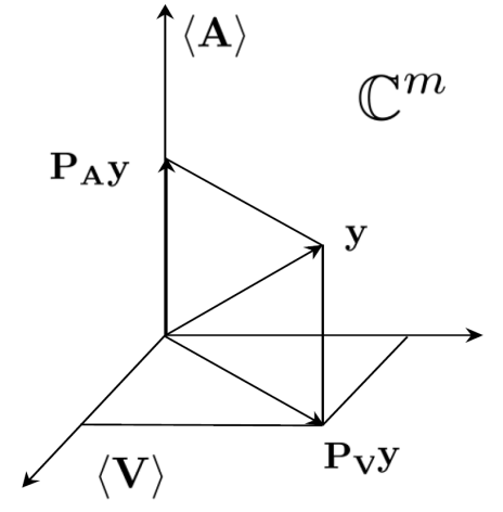
and 𝐏𝐕(𝐳,𝕀)subscript𝐏𝐕𝐳𝕀\mathbf{P}_{{\bf V}({\bf z},\mathbb{I})} and 𝐏𝐀(𝐳,𝕀)=𝐈𝐏𝐕(𝐳,𝕀)subscript𝐏𝐀𝐳𝕀𝐈subscript𝐏𝐕𝐳𝕀\mathbf{P}_{{\bf A}({\bf z},\mathbb{I})}=\mathbf{I}-\mathbf{P}_{{\bf V}({\bf z},\mathbb{I})} are the orthogonal projections onto the column spans of 𝐕(𝐳,𝕀)𝐕𝐳𝕀{\bf V}({\bf z},\mathbb{I}) and 𝐀(𝐳,𝕀)𝐀𝐳𝕀{\bf A}({\bf z},\mathbb{I}), respectively. We denote these column spans by the subspaces 𝐕(𝐳,𝕀)delimited-⟨⟩𝐕𝐳𝕀\langle{\bf V}({\bf z},\mathbb{I})\rangle and 𝐀(𝐳,𝕀)delimited-⟨⟩𝐀𝐳𝕀\langle{\bf A}({\bf z},\mathbb{I})\rangle. We call 𝐕(𝐳,𝕀)delimited-⟨⟩𝐕𝐳𝕀\langle{\bf V}({\bf z},\mathbb{I})\rangle the signal subspace and 𝐀(𝐳,𝕀)delimited-⟨⟩𝐀𝐳𝕀\langle{\bf A}({\bf z},\mathbb{I})\rangle the orthogonal subspace. Note that 𝐀(𝐳,𝕀)=𝐕(𝐳,𝕀)delimited-⟨⟩𝐀𝐳𝕀superscriptdelimited-⟨⟩𝐕𝐳𝕀perpendicular-to\langle{\bf A}({\bf z},\mathbb{I})\rangle=\langle{\bf V}({\bf z},\mathbb{I})\rangle^{\perp}. See Figure 1.

Refer to caption
Figure 1: The signal subspace 𝐕(𝐳,𝕀)delimited-⟨⟩𝐕𝐳𝕀\langle{\bf V}({\bf z},\mathbb{I})\rangle and the orthogonal subspace 𝐀(𝐳,𝕀)=𝐕(𝐳,𝕀)delimited-⟨⟩𝐀𝐳𝕀superscriptdelimited-⟨⟩𝐕𝐳𝕀perpendicular-to\langle{\bf A}({\bf z},\mathbb{I})\rangle=\langle{\bf V}({\bf z},\mathbb{I})\rangle^{\perp}. In the figure, we have dropped (𝐳,,𝕀)({\bf z},,\mathbb{I}) and have simply used 𝐀𝐀{\bf A}, 𝐕𝐕{\bf V}, 𝐀delimited-⟨⟩𝐀\langle{\bf A}\rangle, and 𝐕delimited-⟨⟩𝐕\langle{\bf V}\rangle.

For a given array geometry, the basis matrix 𝐕(𝐳,𝕀)𝐕𝐳𝕀{\bf V}({\bf z},\mathbb{I}) given in (3), and the subspace 𝐕(𝐳,𝕀)delimited-⟨⟩𝐕𝐳𝕀\langle{\bf V}({\bf z},\mathbb{I})\rangle, are fully characterized by the p𝑝p modes 𝐳=[z1,z2,,zp]T𝐳superscriptsubscript𝑧1subscript𝑧2subscript𝑧𝑝𝑇{\bf z}=[z_{1},z_{2},\dots,z_{p}]^{T}. This subspace, parameterized by 𝐳𝐳{\bf z}, is an element of a Grassmanian manifold of dimension p𝑝p. Now, let us rewrite 𝐕(𝐳,𝕀)𝐕𝐳𝕀{\bf V}({\bf z},\mathbb{I}), using elementary operations, and with some abuse of notation, as

𝐕(𝐳,𝕀)=[𝐕1(𝐳,𝕀)𝐕2(𝐳,𝕀)],𝐕𝐳𝕀matrixsubscript𝐕1𝐳𝕀subscript𝐕2𝐳𝕀{\bf V}({\bf z},\mathbb{I})=\begin{bmatrix}{\bf V}_{1}({\bf z},\mathbb{I})\\ {\bf V}_{2}({\bf z},\mathbb{I})\\ \end{bmatrix}, (8)

where 𝐕1(𝐳,𝕀)p×psubscript𝐕1𝐳𝕀superscript𝑝𝑝{\bf V}_{1}({\bf z},\mathbb{I})\in\mathbb{C}^{p\times p} is invertible and 𝐕2(𝐳,𝕀)(mp)×psubscript𝐕2𝐳𝕀superscript𝑚𝑝𝑝{\bf V}_{2}({\bf z},\mathbb{I})\in\mathbb{C}^{(m-p)\times p}. Then the basis matrix 𝐀(𝐳,𝕀)𝐀𝐳𝕀{\bf A}({\bf z},\mathbb{I}) for the orthogonal subspace is the Hermitian transpose of

𝐀H(𝐳,𝕀)=[𝐕2(𝐳,𝕀)𝐕11(𝐳,𝕀)|𝐈mp].superscript𝐀𝐻𝐳𝕀delimited-[]conditionalsubscript𝐕2𝐳𝕀superscriptsubscript𝐕11𝐳𝕀subscript𝐈𝑚𝑝{\bf A}^{H}({\bf z},\mathbb{I})=[-{\bf V}_{2}({\bf z},\mathbb{I}){\bf V}_{1}^{-1}({\bf z},\mathbb{I})\ |\ \mathbf{I}_{m-p}]. (9)

Although these p𝑝p-dimensional characterizations of the signal and orthogonal subspaces have minimum parameterization 𝐳p𝐳superscript𝑝{\bf z}\in\mathbb{C}^{p}, it is not easy to solve the least squares problem (II) using these characterizations.

For an m𝑚m-element uniform line array, a particular p𝑝p-parameter characterization of 𝐀(𝐳,𝕀)𝐀𝐳𝕀{\bf A}({\bf z},\mathbb{I}) exists that makes solving (II) relatively simple [1]. We will review this characterization in Section III. Then, we derive such suitable parameterizations of 𝐀(𝐳,𝕀)𝐀𝐳𝕀{\bf A}({\bf z},\mathbb{I}) for two specific non-uniform arrays: sparse and co-prime.

  • Sparse array: In this case, the location set 𝕀𝕀\mathbb{I} is given by 𝕀s={0,d,2d,,(m2)d,M}subscript𝕀𝑠0𝑑2𝑑𝑚2𝑑𝑀\mathbb{I}_{s}=\{0,d,2d,\dots,(m-2)d,M\}, where M𝑀M and d𝑑d are co-prime integers, that is, (M,d)=1𝑀𝑑1(M,d)=1, and d>1𝑑1d>1. This array may be thought of as two subarrays. The first is a downsampled version, by a factor d𝑑d, of an (m1)d𝑚1𝑑(m-1)d-element uniform line array (ULA) with half wavelength interelement spacings. The second is a single sensor at location M𝑀M in the line array such that M𝑀M and d𝑑d are co-prime. We call this the sparse array because of the single element that sits apart from the origin of the first subarray. We note that M𝑀M need not be greater than (m2)d𝑚2𝑑(m-2)d.

  • Co-prime array: In this case, 𝕀=𝕀1𝕀2𝕀subscript𝕀1subscript𝕀2\mathbb{I}=\mathbb{I}_{1}\cup\mathbb{I}_{2}, where 𝕀1={0,m2,2m2,,(m11)m2}subscript𝕀10subscript𝑚22subscript𝑚2subscript𝑚11subscript𝑚2\mathbb{I}_{1}=\{0,m_{2},2m_{2},\dots,(m_{1}-1)m_{2}\}, 𝕀2={m1,2m1,,(2m21)m1}subscript𝕀2subscript𝑚12subscript𝑚12subscript𝑚21subscript𝑚1\mathbb{I}_{2}=\{m_{1},2m_{1},\dots,(2m_{2}-1)m_{1}\}, and (m1,m2)=1subscript𝑚1subscript𝑚21(m_{1},m_{2})=1. Again the array is composed of two subarrays. The first is an m1subscript𝑚1m_{1}-element ULA with interelement spacings of m2subscript𝑚2m_{2} and sensor locations 𝕀1subscript𝕀1\mathbb{I}_{1}. The second is a (2m21)2subscript𝑚21(2m_{2}-1)-element ULA with interelement spacings of m1subscript𝑚1m_{1} and sensor locations 𝕀2subscript𝕀2\mathbb{I}_{2}. This co-prime geometry was recently introduced in [17] and [18].

Remark 2: In both cases, the co-prime constraint guarantees that aliasing ambiguities due to undersampling can be resolved. Although a sparse array can be viewed as a special case of a co-prime array, we consider them separately, because it is easier to first derive a suitable characterization of the orthogonal subspace 𝐀delimited-⟨⟩𝐀\langle{\bf A}\rangle for a sparse array, and then generalize it to a co-prime array. Our parameterizations are not minimal. They involve 2p2𝑝2p parameters, instead of p𝑝p, but as we will show in Section IV, they are specifically designed to utilize modern methods of linear prediction and approximate least squares, such as IQML.

Remark 3: By now it should be clear that 𝐀(𝐳,𝕀)𝐀𝐳𝕀{\bf A}({\bf z},\mathbb{I}), and therefore its parameterization, depend on both the mode vector 𝐳𝐳{\bf z} and the array geometry 𝕀𝕀\mathbb{I}. Therefore, from here on, we may drop (𝐳,𝕀)𝐳𝕀({\bf z},\mathbb{I}) and simply use 𝐀𝐀{\bf A}, 𝐕𝐕{\bf V}, 𝐀delimited-⟨⟩𝐀\langle{\bf A}\rangle, and 𝐕delimited-⟨⟩𝐕\langle{\bf V}\rangle.

III Characterization of the Orthogonal Subspace for Uniform Line Arrays

Consider a uniform line array of m𝑚m equidistant sensors located at 𝕀u={0,1,2,,m1}subscript𝕀𝑢012𝑚1\mathbb{I}_{u}=\{0,1,2,\dots,m-1\}, taking measurements from the superposition of p𝑝p modes as in (2). The signal subspace in this case is characterized by the Vandermonde matrix 𝐕𝐕{\bf V} in (3) with 𝕀=𝕀u𝕀subscript𝕀𝑢\mathbb{I}=\mathbb{I}_{u}. To characterize the orthogonal subspace 𝐀delimited-⟨⟩𝐀\langle{\bf A}\rangle, consider the polynomial A(z)𝐴𝑧A(z):

A(z)𝐴𝑧\displaystyle A(z) =k=1p(1zkz1)absentsuperscriptsubscriptproduct𝑘1𝑝1subscript𝑧𝑘superscript𝑧1\displaystyle=\prod_{k=1}^{p}(1-z_{k}z^{-1})
=i=0paizi;a0=1formulae-sequenceabsentsuperscriptsubscript𝑖0𝑝subscript𝑎𝑖superscript𝑧𝑖subscript𝑎01\displaystyle=\sum_{i=0}^{p}a_{i}z^{-i};\hskip 14.22636pta_{0}=1 (10)

which has (z1,z2,,zp)subscript𝑧1subscript𝑧2subscript𝑧𝑝(z_{1},z_{2},\dots,z_{p}) as its p𝑝p complex roots. The (mp)𝑚𝑝(m-p) dimensional orthogonal subspace 𝐀delimited-⟨⟩𝐀\langle{\bf A}\rangle is spanned by the mp𝑚𝑝m-p linearly independent columns of 𝐀𝐀{\bf A}:

𝐀=[apap1a11000ap00apa11]H.𝐀superscriptmatrixsubscript𝑎𝑝subscript𝑎𝑝1subscript𝑎11000subscript𝑎𝑝missing-subexpressionmissing-subexpressionmissing-subexpressionmissing-subexpressionmissing-subexpressionmissing-subexpression00subscript𝑎𝑝subscript𝑎11𝐻\mathbf{A}=\begin{bmatrix}a_{p}&a_{p-1}&\cdots&a_{1}&1&0&\cdots&0\\ 0&a_{p}&&&&\ddots&\ddots&\vdots\\ \vdots&\ddots&\ddots&&&&\ddots&\vdots\\ 0&\cdots&0&a_{p}&\cdots&\cdots&a_{1}&1\\ \end{bmatrix}^{H}. (11)

Since 𝐀H𝐕=𝟎superscript𝐀𝐻𝐕0{\bf A}^{H}{\bf V}=\mathbf{0}, and the columns of 𝐀𝐀{\bf A} are linearly independent, 𝐕𝐕{\bf V} and 𝐀𝐀{\bf A} span orthogonal subspaces 𝐕delimited-⟨⟩𝐕\langle{\bf V}\rangle and 𝐀delimited-⟨⟩𝐀\langle{\bf A}\rangle in msuperscript𝑚\mathbb{C}^{m}. The above parameterization is at the heart of methods of linear prediction, approximate least squares, and IQML (see, e.g., [2][5]).

Using the p𝑝p-parameter representation for 𝐀delimited-⟨⟩𝐀\langle{\bf A}\rangle in (11) we may re-write the least squares problem of (II) as

𝐚^=argmin𝐚=[a1,,ap]Tpn=0N1𝐲H[n]𝐏𝐀𝐲[n].^𝐚subscriptargmin𝐚superscriptsubscript𝑎1subscript𝑎𝑝𝑇superscript𝑝superscriptsubscript𝑛0𝑁1superscript𝐲𝐻delimited-[]𝑛subscript𝐏𝐀𝐲delimited-[]𝑛\hat{\mathbf{a}}=\mathop{\mathrm{argmin}}_{\mathbf{a}=[a_{1},\dots,a_{p}]^{T}\in\mathbb{C}^{p}}\sum_{n={\color[rgb]{0,0,0}{0}}}^{{\color[rgb]{0,0,0}{N-1}}}{\bf y}^{H}[n]\mathbf{P}_{{\bf A}}{\bf y}[n]. (12)

There are many algorithms to approximately solve the nonlinear least squares problem in (12). One approach is to ignore the (𝐀H𝐀)1superscriptsuperscript𝐀𝐻𝐀1({\bf A}^{H}{\bf A})^{-1} term in the projection matrix 𝐏𝐀=𝐀(𝐀H𝐀)1𝐀Hsubscript𝐏𝐀𝐀superscriptsuperscript𝐀𝐻𝐀1superscript𝐀𝐻\mathbf{P}_{{\bf A}}={\bf A}({\bf A}^{H}{\bf A})^{-1}{\bf A}^{H} and solve the following modified least squares or linear prediction problem:

𝐚^=argmin𝐚pn=0N1𝐲H[n]𝐀𝐀H𝐲[n].^𝐚subscriptargmin𝐚superscript𝑝superscriptsubscript𝑛0𝑁1superscript𝐲𝐻delimited-[]𝑛superscript𝐀𝐀𝐻𝐲delimited-[]𝑛\displaystyle\hat{\mathbf{a}}=\mathop{\mathrm{argmin}}_{\mathbf{a}\in\mathbb{C}^{p}}\sum_{n={\color[rgb]{0,0,0}{0}}}^{{\color[rgb]{0,0,0}{N-1}}}{\bf y}^{H}[n]{\bf A}{\bf A}^{H}{\bf y}[n]. (13)

The iterative quadratic maximum likelihood (IQML) algorithm (see [2], [3], and [23]) is another method to approximately solve (12). In the l𝑙lth iteration of IQML, the parameters 𝐚lsubscript𝐚𝑙\mathbf{a}_{l} are estimated by iteratively minimizing the quadratic form

𝐚^l=argmin𝐚lp𝐚lH[n=0N1𝐘H[n](𝐀l1H𝐀l1)1𝐘[n]]𝐚l,subscript^𝐚𝑙subscriptargminsubscript𝐚𝑙superscript𝑝superscriptsubscript𝐚𝑙𝐻delimited-[]superscriptsubscript𝑛0𝑁1superscript𝐘𝐻delimited-[]𝑛superscriptsuperscriptsubscript𝐀𝑙1𝐻subscript𝐀𝑙11𝐘delimited-[]𝑛subscript𝐚𝑙\displaystyle\hat{\mathbf{a}}_{l}=\mathop{\mathrm{argmin}}_{\mathbf{a}_{l}\in\mathbb{C}^{p}}~{}\mathbf{a}_{l}^{H}\left[\sum_{n=0}^{N-1}{\bf Y}^{H}[n]({\bf A}_{l-1}^{H}{\bf A}_{l-1})^{-1}{\bf Y}[n]\right]\mathbf{a}_{l}, (14)

where 𝐀l1subscript𝐀𝑙1{\bf A}_{l-1} is formed as in (11) using the estimated parameters 𝐚^l1subscript^𝐚𝑙1\hat{\mathbf{a}}_{l-1} from iteration (l1)𝑙1(l-1) and 𝐲[n]𝐲delimited-[]𝑛{\bf y}[n] is the following (mp)×p𝑚𝑝𝑝(m-p)\times p Hankel data matrix for snapshot n𝑛n:

𝐘[n]=[y0[n]yp1[n]yp[n]y1[n]yp[n]yp+1[n]ym1p[n]ym2[n]ym1[n]].𝐘delimited-[]𝑛matrixsubscript𝑦0delimited-[]𝑛subscript𝑦𝑝1delimited-[]𝑛subscript𝑦𝑝delimited-[]𝑛subscript𝑦1delimited-[]𝑛subscript𝑦𝑝delimited-[]𝑛subscript𝑦𝑝1delimited-[]𝑛missing-subexpressionsubscript𝑦𝑚1𝑝delimited-[]𝑛subscript𝑦𝑚2delimited-[]𝑛subscript𝑦𝑚1delimited-[]𝑛{\bf Y}[n]=\begin{bmatrix}y_{0}[n]&\cdots&y_{p-1}[n]&y_{p}[n]\\ y_{1}[n]&\cdots&y_{p}[n]&y_{p+1}[n]\\ \vdots&&\vdots&\vdots\\ y_{m-1-p}[n]&\cdots&y_{m-2}[n]&y_{m-1}[n]\end{bmatrix}. (15)

After a number of these iterations the sequence {𝐚^l}subscript^𝐚𝑙\{\hat{\mathbf{a}}_{l}\} converges to an estimate 𝐚^=[a^1,,a^p]T\hat{\mathbf{a}}=[\hat{a}_{1},\ldots,\hat{a}_{p}]{\color[rgb]{0,0,0}{{}^{T}}}. The polynomial A^(z)=i=0pa^izi^𝐴𝑧superscriptsubscript𝑖0𝑝subscript^𝑎𝑖superscript𝑧𝑖\hat{A}(z)=\sum_{i=0}^{p}\hat{a}_{i}z^{-i} is then formed from this estimate and its roots are taken as the mode estimates (z^1,z^2,,z^p)subscript^𝑧1subscript^𝑧2subscript^𝑧𝑝(\hat{z}_{1},\hat{z}_{2},\dots,\hat{z}_{p}).

IV Characterization of the Orthogonal Subspaces for Sparse and Co-prime Arrays

In this section, we present simple characterizations of the orthogonal subspace 𝐀delimited-⟨⟩𝐀\langle{\bf A}\rangle for the sparse and co-prime arrays discussed in Section II. Based on our characterizations, we adopt IQML for approximate least squares estimation of complex exponential modes in such arrays.

IV-A Sparse Array

Consider the sparse array described in Section II. The set of sensor locations for this array is 𝕀s={0,d,2d,,(m2)d,M}subscript𝕀𝑠0𝑑2𝑑𝑚2𝑑𝑀\mathbb{I}_{s}=\{0,d,2d,\dots,(m-2)d,M\}. The generalized Vandermonde matrix 𝐕𝐕{\bf V} in this case is

𝐕(𝐳,𝕀s)=[111z1dz2dzpdz1(m2)dz2(m2)dzp(m2)dz1Mz2MzpM].𝐕𝐳subscript𝕀𝑠matrix111superscriptsubscript𝑧1𝑑superscriptsubscript𝑧2𝑑superscriptsubscript𝑧𝑝𝑑superscriptsubscript𝑧1𝑚2𝑑superscriptsubscript𝑧2𝑚2𝑑superscriptsubscript𝑧𝑝𝑚2𝑑superscriptsubscript𝑧1𝑀superscriptsubscript𝑧2𝑀superscriptsubscript𝑧𝑝𝑀{\bf V}({\bf z},\mathbb{I}_{s})=\begin{bmatrix}1&1&\cdots&1\\ z_{1}^{d}&z_{2}^{d}&\cdots&z_{p}^{d}\\ \vdots&\vdots&\ddots&\vdots\\ z_{1}^{(m-2)d}&z_{2}^{(m-2)d}&\cdots&z_{p}^{(m-2)d}\\ z_{1}^{M}&z_{2}^{M}&\cdots&z_{p}^{M}\end{bmatrix}. (16)

For d>1𝑑1d>1 it is clear that without the use of the last sensor at location M𝑀M, we cannot unambiguously estimate the modes, because any two modes zksubscript𝑧𝑘z_{k} and zkej2πq/d,q=1,2,,d1formulae-sequencesubscript𝑧𝑘superscript𝑒𝑗2𝜋𝑞𝑑𝑞12𝑑1z_{k}e^{j2\pi q/d},~{}q=1,2,\cdots,d-1 produce the same measurement. This is the aliasing problem for subsampled arrays.

To characterize the (mp)𝑚𝑝(m-p)-dimensional orthogonal subspace 𝐀delimited-⟨⟩𝐀\langle{\bf A}\rangle, determined by the modes {zk}k=1psuperscriptsubscriptsubscript𝑧𝑘𝑘1𝑝\{z_{k}\}_{k=1}^{p}, we first form the polynomial A(z)𝐴𝑧A(z) from the d𝑑dth powers of zksubscript𝑧𝑘z_{k}, namely the wk=zkdsubscript𝑤𝑘superscriptsubscript𝑧𝑘𝑑w_{k}=z_{k}^{d}, k=1,2,,p𝑘12𝑝k=1,2,\dots,p:

A(z)𝐴𝑧\displaystyle A(z) =k=1p(1wkz1)=i=0paizi;a0=1.formulae-sequenceabsentsuperscriptsubscriptproduct𝑘1𝑝1subscript𝑤𝑘superscript𝑧1superscriptsubscript𝑖0𝑝subscript𝑎𝑖superscript𝑧𝑖subscript𝑎01\displaystyle=\prod_{k=1}^{p}(1-w_{k}z^{-1})=\sum_{i=0}^{p}a_{i}z^{-i};\quad a_{0}=1. (17)

Since {wk}k=1psuperscriptsubscriptsubscript𝑤𝑘𝑘1𝑝\{w_{k}\}_{k=1}^{p} are the roots of A(z)𝐴𝑧A(z), the first mp1𝑚𝑝1m-p-1 columns 𝐀0subscript𝐀0\mathbf{A}_{0} of 𝐀m×(mp)𝐀superscript𝑚𝑚𝑝\mathbf{A}\in\mathbb{C}^{m\times(m-p)}, which is to satisfy 𝐀H𝐕=𝟎superscript𝐀𝐻𝐕0\mathbf{A}^{H}{\bf V}=\mathbf{0}, can be written as

𝐀0H=[apap1a11000ap00apa110].superscriptsubscript𝐀0𝐻matrixsubscript𝑎𝑝subscript𝑎𝑝1subscript𝑎110missing-subexpression00subscript𝑎𝑝missing-subexpressionmissing-subexpressionmissing-subexpressionmissing-subexpressionmissing-subexpressionmissing-subexpressionmissing-subexpressionmissing-subexpression00subscript𝑎𝑝subscript𝑎110\mathbf{A}_{0}^{H}=\begin{bmatrix}a_{p}&a_{p-1}&\cdots&a_{1}&1&0&\cdots&&0\\ 0&a_{p}&&&&\ddots&\ddots&&\vdots\\ \vdots&\ddots&\ddots&&&&\ddots&&\vdots\\ 0&\cdots&0&a_{p}&\cdots&\cdots&a_{1}&1&0\\ \end{bmatrix}. (18)

But of course any mode of the form zkej2πq/dsubscript𝑧𝑘superscript𝑒𝑗2𝜋𝑞𝑑z_{k}e^{j2\pi q/d}, q=1,,d1𝑞1𝑑1q=1,\ldots,d-1, would produce the same wksubscript𝑤𝑘w_{k} and therefore the same 𝐀0subscript𝐀0{\bf A}_{0}. This is the ambiguity caused by aliasing.

Now, consider the polynomial

B(z)=zM+i=1pbiz(pi)d.𝐵𝑧superscript𝑧𝑀superscriptsubscript𝑖1𝑝subscript𝑏𝑖superscript𝑧𝑝𝑖𝑑B(z)=z^{M}+\sum\limits_{i=1}^{p}b_{i}z^{(p-i)d}. (19)

Suppose the coefficient vector 𝐛=[b1,b2,,bp]T𝐛superscriptsubscript𝑏1subscript𝑏2subscript𝑏𝑝𝑇\mathbf{b}=[b_{1},b_{2},\cdots,b_{p}]^{T} is such that the actual modes {zk}k=1psuperscriptsubscriptsubscript𝑧𝑘𝑘1𝑝\{z_{k}\}_{k=1}^{p} are the roots of B(z)𝐵𝑧B(z). That is, B(zk)=0fork=1,2,,pformulae-sequence𝐵subscript𝑧𝑘0for𝑘12𝑝B(z_{k})=0~{}\makebox{for}~{}k=1,2,\dots,p. Then, since M𝑀M and d𝑑d are co-prime, for 1qd11𝑞𝑑11\leq q\leq d-1 and 1kp1𝑘𝑝1\leq k\leq p we have

B(zkej2πq/d)𝐵subscript𝑧𝑘superscript𝑒𝑗2𝜋𝑞𝑑\displaystyle B(z_{k}e^{j2\pi q/d}) =zkMej2πMq/d+i=1pbizk(pi)dabsentsuperscriptsubscript𝑧𝑘𝑀superscript𝑒𝑗2𝜋𝑀𝑞𝑑superscriptsubscript𝑖1𝑝subscript𝑏𝑖superscriptsubscript𝑧𝑘𝑝𝑖𝑑\displaystyle=z_{k}^{M}e^{j2\pi Mq/d}+\sum\limits_{i=1}^{p}b_{i}z_{k}^{(p-i)d}
=zkM(ej2πMq/d1)absentsuperscriptsubscript𝑧𝑘𝑀superscript𝑒𝑗2𝜋𝑀𝑞𝑑1\displaystyle=z_{k}^{M}(e^{j2\pi Mq/d}-1)
0forq=1,2,,d1.formulae-sequenceabsent0for𝑞12𝑑1\displaystyle\neq 0~{}~{}\makebox{for}~{}q=1,2,\dots,d-1. (20)

Therefore, the only common roots of B(z)𝐵𝑧B(z), and the d𝑑dth roots of {wk}k=1psuperscriptsubscriptsubscript𝑤𝑘𝑘1𝑝\{w_{k}\}_{k=1}^{p}, are {zk}k=1psuperscriptsubscriptsubscript𝑧𝑘𝑘1𝑝\{z_{k}\}_{k=1}^{p}, which are the actual modes to be estimated. In this way, B(z)𝐵𝑧B(z) resolves the ambiguities.

Now suppose {wk}k=1psuperscriptsubscriptsubscript𝑤𝑘𝑘1𝑝\{w_{k}\}_{k=1}^{p} are known (or estimated). Then from (19), 𝐛𝐛\mathbf{b} can be found by solving the linear system of equations

(bpbp1b1)(111z1dz2dzpdz1(p1)dz2(p1)dzp(p1)d)=(z1Mz2MzpM),matrixsubscript𝑏𝑝subscript𝑏𝑝1subscript𝑏1matrix111superscriptsubscript𝑧1𝑑superscriptsubscript𝑧2𝑑superscriptsubscript𝑧𝑝𝑑superscriptsubscript𝑧1𝑝1𝑑superscriptsubscript𝑧2𝑝1𝑑superscriptsubscript𝑧𝑝𝑝1𝑑matrixsuperscriptsubscript𝑧1𝑀superscriptsubscript𝑧2𝑀superscriptsubscript𝑧𝑝𝑀\begin{pmatrix}b_{p}&b_{p-1}&\ldots&b_{1}\end{pmatrix}\begin{pmatrix}1&1&\cdots&1\\ z_{1}^{d}&z_{2}^{d}&\cdots&z_{p}^{d}\\ \vdots&\vdots&\ddots&\vdots\\ z_{1}^{(p-1)d}&z_{2}^{(p-1)d}&\cdots&z_{p}^{(p-1)d}\end{pmatrix}=-\begin{pmatrix}z_{1}^{M}&z_{2}^{M}&\ldots&z_{p}^{M}\end{pmatrix}, (21)

which if zidzjdsuperscriptsubscript𝑧𝑖𝑑superscriptsubscript𝑧𝑗𝑑z_{i}^{d}\neq z_{j}^{d} for ij𝑖𝑗i\neq j (as we assume) has a unique solution.

Using the 2p2𝑝2p coefficients {ai}i=1psuperscriptsubscriptsubscript𝑎𝑖𝑖1𝑝\{a_{i}\}_{i=1}^{p} and {bi}i=1psuperscriptsubscriptsubscript𝑏𝑖𝑖1𝑝\{b_{i}\}_{i=1}^{p}, we can characterize 𝐀delimited-⟨⟩𝐀\langle{\bf A}\rangle by writing 𝐀m×(mp)𝐀superscript𝑚𝑚𝑝{\bf A}\in\mathbb{C}^{m\times(m-p)} as

𝐀=[apap1a11000ap00apa110bpbp1b1001]H.𝐀superscriptmatrixsubscript𝑎𝑝subscript𝑎𝑝1subscript𝑎11000subscript𝑎𝑝missing-subexpressionmissing-subexpressionmissing-subexpressionmissing-subexpressionmissing-subexpressionmissing-subexpression00subscript𝑎𝑝subscript𝑎110subscript𝑏𝑝subscript𝑏𝑝1subscript𝑏1001𝐻\mathbf{A}=\begin{bmatrix}a_{p}&a_{p-1}&\cdots&a_{1}&1&0&\cdots&0\\ 0&a_{p}&&&&\ddots&\ddots&\vdots\\ \vdots&\ddots&\ddots&&&&\ddots&\vdots\\ 0&\cdots&0&a_{p}&\cdots&a_{1}&1&0\\ b_{p}&b_{p-1}&\cdots&b_{1}&0&\cdots&0&1\end{bmatrix}^{H}. (22)

To estimate 𝐚=[a1,,ap]T𝐚superscriptsubscript𝑎1subscript𝑎𝑝𝑇\mathbf{a}=[a_{1},\cdots,a_{p}]^{T} and 𝐛=[b1,,bp]T𝐛superscriptsubscript𝑏1subscript𝑏𝑝𝑇\mathbf{b}=[b_{1},\cdots,b_{p}]^{T}, we need to solve the following problem:

min𝐚,𝐛n=0N1𝐲H[n]𝐏𝐀𝐲[n],subscript𝐚𝐛superscriptsubscript𝑛0𝑁1superscript𝐲𝐻delimited-[]𝑛subscript𝐏𝐀𝐲delimited-[]𝑛\displaystyle\min_{\mathbf{a,b}}\sum_{n=0}^{N-1}{\bf y}^{H}[n]\mathbf{P}_{{\bf A}}{\bf y}[n], (23)

We approximate the solution to this problem in two steps. First, we ignore the last column of 𝐀𝐀{\bf A} and estimate 𝐚𝐚\mathbf{a} as

𝐚^=argmin𝐚n=0N1𝐲H[n]𝐏𝐀0𝐲[n].^𝐚subscriptargmin𝐚superscriptsubscript𝑛0𝑁1superscript𝐲𝐻delimited-[]𝑛subscript𝐏subscript𝐀0𝐲delimited-[]𝑛\displaystyle\hat{\mathbf{a}}=\mathop{\mathrm{argmin}}_{\mathbf{a}}\sum_{n=0}^{N-1}{\bf y}^{H}[n]\mathbf{P}_{{\bf A}_{0}}{\bf y}[n]. (24)

In the noiseless case, where the 𝐲[n]𝐲delimited-[]𝑛{\bf y}[n], n=0,1,,N1𝑛01𝑁1n=0,1,\ldots,N-1, lie in 𝐕delimited-⟨⟩𝐕\langle{\bf V}\rangle, it can be shown that if m2p+1𝑚2𝑝1m\geq 2p+1 then the solution to (24) is unique and yields the coefficients of the polynomial A(z)𝐴𝑧A(z) with roots (w1,w2,,wp)subscript𝑤1subscript𝑤2subscript𝑤𝑝(w_{1},w_{2},\dots,w_{p}). See Appendix A.

The minimization problem in (24) can be solved using IQML. Now, given 𝐚^^𝐚\hat{\mathbf{a}}, we form the polynomial

A^(z)^𝐴𝑧\displaystyle\hat{A}(z) =1+i=1pa^iziabsent1superscriptsubscript𝑖1𝑝subscript^𝑎𝑖superscript𝑧𝑖\displaystyle=1+\sum_{i=1}^{p}\hat{a}_{i}z^{-i}
=k=1p(1w^kz1)absentsuperscriptsubscriptproduct𝑘1𝑝1subscript^𝑤𝑘superscript𝑧1\displaystyle=\prod_{k=1}^{p}(1-\hat{w}_{k}z^{-1}) (25)

and derive its roots as {w^k}k=1psuperscriptsubscriptsubscript^𝑤𝑘𝑘1𝑝\{\hat{w}_{k}\}_{k=1}^{p}. But we know from the structure of the problem that w^k=z^kdsubscript^𝑤𝑘superscriptsubscript^𝑧𝑘𝑑\hat{w}_{k}=\hat{z}_{k}^{d}, and any of the d𝑑d-th roots of z^kdsuperscriptsubscript^𝑧𝑘𝑑\hat{z}_{k}^{d} is a candidate solution. Therefore, we construct the candidate set,

={\displaystyle\mathcal{R}=\{ (z^1ej2πq1/d,z^2ej2πq2/d,,z^pej2πqp/d)|0q1,q2,,qpd1},\displaystyle(\hat{z}_{1}e^{j2\pi q_{1}/d},\hat{z}_{2}e^{j2\pi q_{2}/d},\cdots,\hat{z}_{p}e^{j2\pi q_{p}/d})|0\leq q_{1},q_{2},\dots,q_{p}\leq d-1\}, (26)

which contains all modes and their aliased versions.

In the second step, to find the p𝑝p actual modes and resolve aliasing ambiguities, we solve the following constrained linear prediction problem:

𝐛^^𝐛\displaystyle\mathbf{\hat{b}} =argmin𝜻n=0N1|ym1[n]+𝜻T𝐮[n]|2absentsubscriptargmin𝜻superscriptsubscript𝑛0𝑁1superscriptsubscript𝑦𝑚1delimited-[]𝑛superscript𝜻𝑇𝐮delimited-[]𝑛2\displaystyle=\mathop{\mathrm{argmin}}_{\bm{\zeta}}\sum_{n=0}^{N-1}|y_{m-1}[n]+\bm{\zeta}^{T}\mathbf{u}[n]|^{2}
s.t.B𝜻(𝐳^)=0,𝐳^,\displaystyle\mathrm{s.t.}\ \ B_{\bm{\zeta}}(\hat{{\bf z}})=0,\ \ \hat{{\bf z}}\in\mathcal{R}, (27)

where 𝐮[n]=[y0[n],y1[n],,yp1[n]]T𝐮delimited-[]𝑛superscriptsubscript𝑦0delimited-[]𝑛subscript𝑦1delimited-[]𝑛subscript𝑦𝑝1delimited-[]𝑛𝑇\mathbf{u}[n]=[y_{0}[n],y_{1}[n],\dots,y_{p-1}[n]]^{T}, and the polynomial B𝜻(z)subscript𝐵𝜻𝑧B_{\bm{\zeta}}(z) is obtained from replacing 𝐛𝐛\mathbf{b} by 𝜻𝜻\bm{\zeta} in (19).

In the noiseless case, where 𝐲[n]𝐲delimited-[]𝑛{\bf y}[n], n=0,1,,N1𝑛01𝑁1n=0,1,\ldots,N-1 lie in 𝐕delimited-⟨⟩𝐕\langle{\bf V}\rangle, the solution 𝐛^^𝐛\hat{\mathbf{b}} to (IV-A) satisfies (21) and yields the actual modes. See Appendix B.

Our algorithm for estimating modes in a sparse array may be summarized in the following steps:

  1. 1.

    Estimate 𝐚^=[a^1,a^2,,a^p]T^𝐚superscriptsubscript^𝑎1subscript^𝑎2subscript^𝑎𝑝𝑇\hat{\mathbf{a}}=[\hat{a}_{1},\hat{a}_{2},\dots,\hat{a}_{p}]^{T} from (24) using IQML;

  2. 2.

    Root A^(z)^𝐴𝑧\hat{A}(z) to return roots {w^k}k=1psuperscriptsubscriptsubscript^𝑤𝑘𝑘1𝑝\{\hat{w}_{k}\}_{k=1}^{p}. Then, recognizing that the d𝑑dth roots of w^ksubscript^𝑤𝑘\hat{w}_{k} are z^kej2πq/dsubscript^𝑧𝑘superscript𝑒𝑗2𝜋𝑞𝑑\hat{z}_{k}e^{j2\pi q/d} for some q{0,1,2,,d1}𝑞012𝑑1q\in\{0,1,2,\dots,d-1\}, form the set of candidate modes \mathcal{R} as in (26);

  3. 3.

    Solve (IV-A) for 𝐛^^𝐛\hat{\mathbf{b}};

  4. 4.

    Intersect the roots of B^(z)^𝐵𝑧\hat{B}(z) with \mathcal{R}.

IV-B Co-prime Array

Consider an m=m1+2m21𝑚subscript𝑚12subscript𝑚21m=m_{1}+2m_{2}-1 element co-prime array, consisting of two uniform subarrays: one with m1subscript𝑚1m_{1} elements at locations 𝕀1={0,m2,2m2,,(m11)m2}subscript𝕀10subscript𝑚22subscript𝑚2subscript𝑚11subscript𝑚2\mathbb{I}_{1}=\{0,m_{2},2m_{2},\dots,(m_{1}-1)m_{2}\} and the other with 2m212subscript𝑚212m_{2}-1 elements at locations 𝕀2={m1,2m1,,(2m21)m1}subscript𝕀2subscript𝑚12subscript𝑚12subscript𝑚21subscript𝑚1\mathbb{I}_{2}=\{m_{1},2m_{1},\dots,(2m_{2}-1)m_{1}\}, where (m1,m2)=1subscript𝑚1subscript𝑚21(m_{1},m_{2})=1 and m1>m2subscript𝑚1subscript𝑚2m_{1}>m_{2}. In this case, the generalized Vandermonde matrix 𝐕m×p𝐕superscript𝑚𝑝{\bf V}\in\mathbb{C}^{m\times p} of modes may be partitioned as

𝐕=[𝐕(𝐳,𝕀1)𝐕(𝐳,𝕀2)],𝐕matrix𝐕𝐳subscript𝕀1𝐕𝐳subscript𝕀2{\bf V}=\begin{bmatrix}{\bf V}({\bf z},\mathbb{I}_{1})\\ {\bf V}({\bf z},\mathbb{I}_{2})\end{bmatrix}, (28)

where

𝐕(𝐳,𝕀1)=[111z1m2z2m2zpm2z12m2z22m2zp2m2z1(m11)m2z2(m11)m2zp(m11)m2]𝐕𝐳subscript𝕀1matrix111superscriptsubscript𝑧1subscript𝑚2superscriptsubscript𝑧2subscript𝑚2superscriptsubscript𝑧𝑝subscript𝑚2superscriptsubscript𝑧12subscript𝑚2superscriptsubscript𝑧22subscript𝑚2superscriptsubscript𝑧𝑝2subscript𝑚2superscriptsubscript𝑧1subscript𝑚11subscript𝑚2superscriptsubscript𝑧2subscript𝑚11subscript𝑚2superscriptsubscript𝑧𝑝subscript𝑚11subscript𝑚2{\bf V}({\bf z},\mathbb{I}_{1})=\begin{bmatrix}1&1&\cdots&1\\ z_{1}^{m_{2}}&z_{2}^{m_{2}}&\cdots&z_{p}^{m_{2}}\\ z_{1}^{2m_{2}}&z_{2}^{2m_{2}}&\cdots&z_{p}^{2m_{2}}\\ \vdots&\vdots&\ddots&\vdots\\ z_{1}^{(m_{1}-1)m_{2}}&z_{2}^{(m_{1}-1)m_{2}}&\cdots&z_{p}^{(m_{1}-1)m_{2}}\\ \end{bmatrix} (29)

and

𝐕(𝐳,𝕀2)=[z1m1z2m1zpm1z12m1z22m1zp2m1z1(2m21)m1z2(2m21)m1zp(2m21)m1]𝐕𝐳subscript𝕀2matrixsuperscriptsubscript𝑧1subscript𝑚1superscriptsubscript𝑧2subscript𝑚1superscriptsubscript𝑧𝑝subscript𝑚1superscriptsubscript𝑧12subscript𝑚1superscriptsubscript𝑧22subscript𝑚1superscriptsubscript𝑧𝑝2subscript𝑚1superscriptsubscript𝑧12subscript𝑚21subscript𝑚1superscriptsubscript𝑧22subscript𝑚21subscript𝑚1superscriptsubscript𝑧𝑝2subscript𝑚21subscript𝑚1{\bf V}({\bf z},\mathbb{I}_{2})=\begin{bmatrix}z_{1}^{m_{1}}&z_{2}^{m_{1}}&\cdots&z_{p}^{m_{1}}\\ z_{1}^{2m_{1}}&z_{2}^{2m_{1}}&\cdots&z_{p}^{2m_{1}}\\ \vdots&\vdots&\ddots&\vdots\\ z_{1}^{(2m_{2}-1)m_{1}}&z_{2}^{(2m_{2}-1)m_{1}}&\cdots&z_{p}^{(2m_{2}-1)m_{1}}\\ \end{bmatrix} (30)

are the Vandermonde matrices for the two individual subarrays of the co-prime array.

Let 𝐀1m1×(m1p)subscript𝐀1superscriptsubscript𝑚1subscript𝑚1𝑝{\bf A}_{1}\in\mathbb{C}^{m_{1}\times(m_{1}-p)} and 𝐁1(2m21)×(2m21p)subscript𝐁1superscript2subscript𝑚212subscript𝑚21𝑝\mathbf{B}_{1}\in\mathbb{C}^{(2m_{2}-1)\times(2m_{2}-1-p)} be matrices that are orthogonal to 𝐕(𝐳,𝕀1)𝐕𝐳subscript𝕀1{\bf V}({\bf z},\mathbb{I}_{1}) and 𝐕(𝐳,𝕀2)𝐕𝐳subscript𝕀2{\bf V}({\bf z},\mathbb{I}_{2}), respectively. That is, 𝐀1H𝐕(𝐳,𝕀1)=𝟎superscriptsubscript𝐀1𝐻𝐕𝐳subscript𝕀10{\bf A}_{1}^{H}{\bf V}({\bf z},\mathbb{I}_{1})=\mathbf{0} and 𝐁1H𝐕(𝐳,𝕀2)=𝟎superscriptsubscript𝐁1𝐻𝐕𝐳subscript𝕀20\mathbf{B}_{1}^{H}{\bf V}({\bf z},\mathbb{I}_{2})=\mathbf{0}. Following our results in the sparse case, we may parameterize 𝐀1m1×(m1p)subscript𝐀1superscriptsubscript𝑚1subscript𝑚1𝑝{\bf A}_{1}\in\mathbb{C}^{m_{1}\times(m_{1}-p)} as

𝐀1H=[apap1a1100ap000apa11],superscriptsubscript𝐀1𝐻matrixsubscript𝑎𝑝subscript𝑎𝑝1subscript𝑎1100subscript𝑎𝑝missing-subexpressionmissing-subexpression0missing-subexpressionmissing-subexpression00subscript𝑎𝑝subscript𝑎11\mathbf{A}_{1}^{H}=\begin{bmatrix}a_{p}&a_{p-1}&\cdots&a_{1}&1&\cdots&0\\ 0&a_{p}&\cdots&&&\cdots&0\\ \vdots&\ddots&\ddots&&\cdots&&\vdots\\ 0&\cdots&0&a_{p}&\cdots&a_{1}&1\\ \end{bmatrix}, (31)

where {ai}i=1psuperscriptsubscriptsubscript𝑎𝑖𝑖1𝑝\{a_{i}\}_{i=1}^{p} are the coefficients of a polynomial A(z)𝐴𝑧A(z), whose roots are wk=zkm2subscript𝑤𝑘superscriptsubscript𝑧𝑘subscript𝑚2w_{k}=z_{k}^{m_{2}}, k=1,2,,p𝑘12𝑝k=1,2,\dots,p. That is,

A(z)𝐴𝑧\displaystyle A(z) =k=1p(1wkz1)absentsuperscriptsubscriptproduct𝑘1𝑝1subscript𝑤𝑘superscript𝑧1\displaystyle=\prod_{k=1}^{p}(1-w_{k}z^{-1})
=i=0paizi,a0=1.formulae-sequenceabsentsuperscriptsubscript𝑖0𝑝subscript𝑎𝑖superscript𝑧𝑖subscript𝑎01\displaystyle=\sum_{i=0}^{p}a_{i}z^{-i},\ \ a_{0}=1. (32)

Similarly, we parameterize 𝐁1(2m21)×(2m21p)subscript𝐁1superscript2subscript𝑚212subscript𝑚21𝑝{\bf B}_{1}\in\mathbb{C}^{(2m_{2}-1)\times(2m_{2}-1-p)} as

𝐁1H=[bpbp1b1100bp000bpb11],superscriptsubscript𝐁1𝐻matrixsubscript𝑏𝑝subscript𝑏𝑝1subscript𝑏1100subscript𝑏𝑝missing-subexpressionmissing-subexpression0missing-subexpressionmissing-subexpression00subscript𝑏𝑝subscript𝑏11\mathbf{B}_{1}^{H}=\begin{bmatrix}b_{p}&b_{p-1}&\cdots&b_{1}&1&\cdots&0\\ 0&b_{p}&\cdots&&&\cdots&0\\ \vdots&\ddots&\ddots&&\cdots&&\vdots\\ 0&\cdots&0&b_{p}&\cdots&b_{1}&1\\ \end{bmatrix}, (33)

where {bi}i=1psuperscriptsubscriptsubscript𝑏𝑖𝑖1𝑝\{b_{i}\}_{i=1}^{p} are the coefficients of a polynomial B(z)𝐵𝑧B(z), whose roots are sk=zkm1subscript𝑠𝑘superscriptsubscript𝑧𝑘subscript𝑚1s_{k}=z_{k}^{m_{1}}, k=1,2,,p𝑘12𝑝k=1,2,\dots,p. That is,

B(z)𝐵𝑧\displaystyle B(z) =k=1p(1skz1)absentsuperscriptsubscriptproduct𝑘1𝑝1subscript𝑠𝑘superscript𝑧1\displaystyle=\prod_{k=1}^{p}(1-s_{k}z^{-1})
=i=0pbizi,b0=1.formulae-sequenceabsentsuperscriptsubscript𝑖0𝑝subscript𝑏𝑖superscript𝑧𝑖subscript𝑏01\displaystyle=\sum_{i=0}^{p}b_{i}z^{-i},\ \ b_{0}=1. (34)

Note that we still need p𝑝p more independent columns to fully characterize the basis matrix 𝐀𝐀{\bf A} for the orthogonal subspace 𝐀delimited-⟨⟩𝐀\langle{\bf A}\rangle. However, using our partial characterization, we can estimate the modes (with no aliasing ambiguities) in the following steps:

  1. 1.

    Separate the measurements of the two subarrays as 𝐮[n]={𝐲i[n]|i𝕀1}𝐮delimited-[]𝑛conditional-setsubscript𝐲𝑖delimited-[]𝑛𝑖subscript𝕀1\mathbf{u}[n]=\{{\bf y}_{i}[n]|i\in\mathbb{I}_{1}\} and 𝐯[n]={𝐲i[n]|i𝕀2}𝐯delimited-[]𝑛conditional-setsubscript𝐲𝑖delimited-[]𝑛𝑖subscript𝕀2\mathbf{v}[n]=\{{\bf y}_{i}[n]|i\in\mathbb{I}_{2}\};

  2. 2.

    Estimate 𝐚^=[a^1,a^2,,a^p]T^𝐚superscriptsubscript^𝑎1subscript^𝑎2subscript^𝑎𝑝𝑇\hat{\mathbf{a}}=[\hat{a}_{1},\hat{a}_{2},\dots,\hat{a}_{p}]^{T} using IQML on 𝐮[n]𝐮delimited-[]𝑛\mathbf{u}[n];

  3. 3.

    Root A^(z)^𝐴𝑧\hat{A}(z) to return the roots {w^k}k=1psuperscriptsubscriptsubscript^𝑤𝑘𝑘1𝑝\{\hat{w}_{k}\}_{k=1}^{p}. Then, recognizing that the m2subscript𝑚2m_{2}th roots of w^ksubscript^𝑤𝑘\hat{w}_{k} are z^kej2πq/m2subscript^𝑧𝑘superscript𝑒𝑗2𝜋𝑞subscript𝑚2\hat{z}_{k}e^{j2\pi q/m_{2}} for some q{0,1,,m21}𝑞01subscript𝑚21q\in\{0,1,\dots,m_{2}-1\}, form the set of candidate modes 1subscript1\mathcal{R}_{1} as

    1={(z^1ej2πk1/m2,z^2ej2πk2/m2,,z^pej2πkp/m2)|0k1,k2,,kpm21};subscript1conditional-setsubscript^𝑧1superscript𝑒𝑗2𝜋subscript𝑘1subscript𝑚2subscript^𝑧2superscript𝑒𝑗2𝜋subscript𝑘2subscript𝑚2subscript^𝑧𝑝superscript𝑒𝑗2𝜋subscript𝑘𝑝subscript𝑚2formulae-sequence0subscript𝑘1subscript𝑘2subscript𝑘𝑝subscript𝑚21\mathcal{R}_{1}=\{(\hat{z}_{1}e^{j2\pi k_{1}/m_{2}},\hat{z}_{2}e^{j2\pi k_{2}/m_{2}},\cdots,\hat{z}_{p}e^{j2\pi k_{p}/m_{2}})\hskip 5.69054pt|\hskip 5.69054pt0\leq k_{1},k_{2},\dots,k_{p}\leq m_{2}-1\}; (35)
  4. 4.

    Estimate 𝐛^=[b^1,b^2,,b^p]T^𝐛superscriptsubscript^𝑏1subscript^𝑏2subscript^𝑏𝑝𝑇\hat{\mathbf{b}}=[\hat{b}_{1},\hat{b}_{2},\dots,\hat{b}_{p}]^{T} using IQML on 𝐯[n]𝐯delimited-[]𝑛\mathbf{v}[n];

  5. 5.

    Root B^(z)^𝐵𝑧\hat{B}(z) to return the roots {s^k}k=1psuperscriptsubscriptsubscript^𝑠𝑘𝑘1𝑝\{\hat{s}_{k}\}_{k=1}^{p}. Then, recognizing that the m1subscript𝑚1m_{1}th roots of s^ksubscript^𝑠𝑘\hat{s}_{k} are z^kej2πq/m1subscript^𝑧𝑘superscript𝑒𝑗2𝜋𝑞subscript𝑚1\hat{z}_{k}e^{j2\pi q/m_{1}} for some q{0,1,,m11}𝑞01subscript𝑚11q\in\{0,1,\dots,m_{1}-1\}, form the set of candidate modes 2subscript2\mathcal{R}_{2} as

    2={(z^1ej2πk1/m1,z^2ej2πk2/m1,,z^pej2πkp/m1)|0k1,k2,,kpm11};subscript2conditional-setsubscript^𝑧1superscript𝑒𝑗2𝜋subscript𝑘1subscript𝑚1subscript^𝑧2superscript𝑒𝑗2𝜋subscript𝑘2subscript𝑚1subscript^𝑧𝑝superscript𝑒𝑗2𝜋subscript𝑘𝑝subscript𝑚1formulae-sequence0subscript𝑘1subscript𝑘2subscript𝑘𝑝subscript𝑚11\mathcal{R}_{2}=\{(\hat{z}_{1}e^{j2\pi k_{1}/m_{1}},\hat{z}_{2}e^{j2\pi k_{2}/m_{1}},\cdots,\hat{z}_{p}e^{j2\pi k_{p}/m_{1}})\hskip 5.69054pt|\hskip 5.69054pt0\leq k_{1},k_{2},\dots,k_{p}\leq m_{1}-1\}; (36)
  6. 6.

    Intersect 1subscript1\mathcal{R}_{1} and 2subscript2\mathcal{R}_{2}, in other words look for the closest (based on the Euclidean metric) p𝑝p members of the set 1subscript1\mathcal{R}_{1} to the set 2subscript2\mathcal{R}_{2}.

Remark 4: To complete the 2plimit-from2𝑝2p-parameterization of the basis matrix 𝐀𝐀{\bf A} for the orthogonal subspace 𝐀delimited-⟨⟩𝐀\langle{\bf A}\rangle, consider the standard representation of 𝐀𝐀{\bf A} given in (9). Define 𝐕1=𝐕(𝐳,𝕀p1)subscript𝐕1𝐕𝐳subscript𝕀subscript𝑝1{\bf V}_{1}={\bf V}({\bf z},\mathbb{I}_{p_{1}}) and 𝐕2=𝐕(𝐳,𝕀p2)subscript𝐕2𝐕𝐳subscript𝕀subscript𝑝2{\bf V}_{2}={\bf V}({\bf z},\mathbb{I}_{p_{2}}) where 𝕀p1={0,m2,,(p1)m2}subscript𝕀subscript𝑝10subscript𝑚2𝑝1subscript𝑚2\mathbb{I}_{p_{1}}=\{0,m_{2},\dots,(p-1)m_{2}\} and 𝕀p2={m1,2m1,,pm1}subscript𝕀subscript𝑝2subscript𝑚12subscript𝑚1𝑝subscript𝑚1\mathbb{I}_{p_{2}}=\{m_{1},2m_{1},\dots,pm_{1}\}. Then, from (9) the p𝑝p remaining columns of 𝐀𝐀{\bf A} may be represented in 𝐂1n×psubscript𝐂1superscript𝑛𝑝\mathbf{C}_{1}\in\mathbb{C}^{n\times p} as:

𝐂1H=[𝐂0H|𝟎p×(m1p)|𝐈p|𝟎p×(2m21p)]superscriptsubscript𝐂1𝐻delimited-[]conditionalsuperscriptsubscript𝐂0𝐻subscript0𝑝subscript𝑚1𝑝subscript𝐈𝑝subscript0𝑝2subscript𝑚21𝑝{\bf C}_{1}^{H}=[\mathbf{C}_{0}^{H}|\hskip 5.69054pt\mathbf{0}_{p\times(m_{1}-p)}\hskip 2.84526pt|\hskip 5.69054pt\mathbf{I}_{p}\hskip 2.84526pt|\hskip 5.69054pt\mathbf{0}_{p\times(2m_{2}-1-p)}] (37)

where 𝟎k×lsubscript0𝑘𝑙\mathbf{0}_{k\times l} denotes a k×l𝑘𝑙k\times l matrix with zero entries, 𝐈psubscript𝐈𝑝\mathbf{I}_{p} is the p×p𝑝𝑝p\times p identity matrix, and

𝐂0H=𝐕(𝐳,𝕀p2)𝐕1(𝐳,𝕀p1)p×p.superscriptsubscript𝐂0𝐻𝐕𝐳subscript𝕀subscript𝑝2superscript𝐕1𝐳subscript𝕀subscript𝑝1superscript𝑝𝑝{\bf C}_{0}^{H}=-{\bf V}({\bf z},\mathbb{I}_{p_{2}}){\bf V}^{-1}({\bf z},\mathbb{I}_{p_{1}})\in\mathbb{C}^{p\times p}. (38)

From (37) and (38) we can see that 𝐂1subscript𝐂1\mathbf{C}_{1} only depends on {zkm1}k=1psuperscriptsubscriptsuperscriptsubscript𝑧𝑘subscript𝑚1𝑘1𝑝\{z_{k}^{m_{1}}\}_{k=1}^{p} and {zkm2}k=1psuperscriptsubscriptsuperscriptsubscript𝑧𝑘subscript𝑚2𝑘1𝑝\{z_{k}^{m_{2}}\}_{k=1}^{p} which are obtained from 𝐚𝐚\mathbf{a} and 𝐛𝐛\mathbf{b} by rooting A𝐚(z)subscript𝐴𝐚𝑧A_{\mathbf{a}}(z) and B𝐛(z)subscript𝐵𝐛𝑧B_{\mathbf{b}}(z) in (IV-B) and (IV-B), respectively. Therefore, the full, and minimally parameterized, characterization of the orthogonal subspace for the co-prime array may be written as

𝐀=[𝐀10𝐂10𝐁1].𝐀delimited-[]subscript𝐀10missing-subexpressionmissing-subexpressionmissing-subexpressionsubscript𝐂10subscript𝐁1missing-subexpression{\bf A}=\left[\begin{array}[]{cc|c}{\bf A}_{1}&0&\vspace{-3mm}\hfil\\ &&{\bf C}_{1}\vspace{-3mm}\\ 0&{\bf B}_{1}&\end{array}\right]. (39)

We note that we do not need this full characterization for estimating the modes. The partial characterization using 𝐀1subscript𝐀1{\bf A}_{1} and 𝐁1subscript𝐁1{\bf B}_{1} suffices, at the expense of p𝑝p fitting equations.

V Numerical Results

In this section we present numerical results for the estimation of damped complex exponential modes in co-prime, sparse and uniform line arrays. We consider a ULA of 505050 elements. We form our co-prime and sparse arrays with 141414 elements by subsampling this ULA. For the sparse array, we subsample the measurements of the ULA by a factor of d=4𝑑4d=4 and place a sensor at M=3𝑀3M=3. For the co-prime array, the first subarray includes m1=7subscript𝑚17m_{1}=7 elements with interelement spacing of m2=4subscript𝑚24m_{2}=4, and the second subarray includes 2m21=72subscript𝑚2172m_{2}-1=7 elements with interelement spacing of m1=7subscript𝑚17m_{1}=7.

It is insightful to first look at the beampatterns of sparse, co-prime, and uniform line arrays for the problem of estimating undamped modes. In this case, the beam pattern B(θ)𝐵𝜃B(\theta) is

B(θ)=l=0m1ejilθ.𝐵𝜃superscriptsubscript𝑙0𝑚1superscript𝑒𝑗subscript𝑖𝑙𝜃B(\theta)=\sum_{l=0}^{m-1}e^{ji_{l}\theta}. (40)

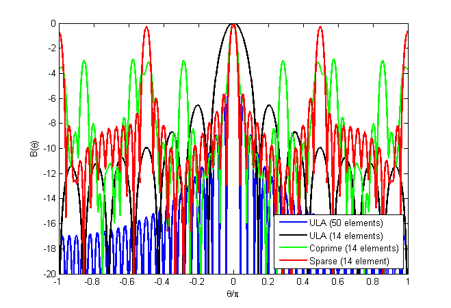
Figure 2 shows the beam patterns for different array geometries. Although the co-prime and sparse arrays of 141414 elements have the same aperture and the same main lobe width as the ULA with 505050 elements, we see that they suffer from higher sidelobes, suggesting that there will be performance losses in resolving closely spaced modes using these arrays, relative to the ULA.
Refer to caption
Figure 2: Beampatterns for ULAs with 141414 and 505050 elements, a sparse array with 141414 elements, d=4𝑑4d=4, and M=3𝑀3M=3, and a co-prime array with 141414 elements, m1=7subscript𝑚17m_{1}=7, and m2=4subscript𝑚24m_{2}=4.

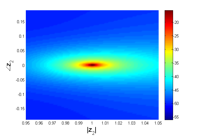
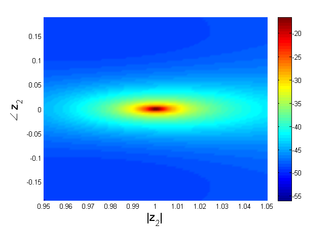
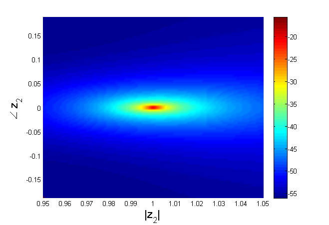
Let us also look at numerical results for the Cramér-Rao bound (CRB) associated with the co-prime, sparse and uniform line arrays (See Appendix C). Figure 3 shows the CRB in the estimation of the mode z1=1subscript𝑧11z_{1}=1 in the presence of an interfering mode z2subscript𝑧2z_{2}. The per sensor SNR is 101010 dB. As the interfering mode z2subscript𝑧2z_{2} gets closer to z1subscript𝑧1z_{1}, the CRB in the estimation of the z1subscript𝑧1z_{1} increases. The CRB for the sparse and co-prime arrays are similar, but they are higher than the CRB for the ULA. Since the aperture of the three arrays are equal, the fewer number of sensors in the sparse and co-prime arrays can be considered the only reason for this difference in the CRB.
Refer to caption
(a) ULA
Refer to caption
(b) Sparse array
Refer to caption
(c) Co-prime array
Figure 3: The CRB in dB for estimating z1=1subscript𝑧11z_{1}=1 in the presence of an interfering mode z2subscript𝑧2z_{2}: (a) ULA with 505050 elements. (b) sparse array with 141414 elements d=4𝑑4d=4 and M=3𝑀3M=3. (c) co-prime array with 232323 elements m1=7subscript𝑚17m_{1}=7 and m2=4subscript𝑚24m_{2}=4. For all arrays per sensor SNR is 101010 dB.

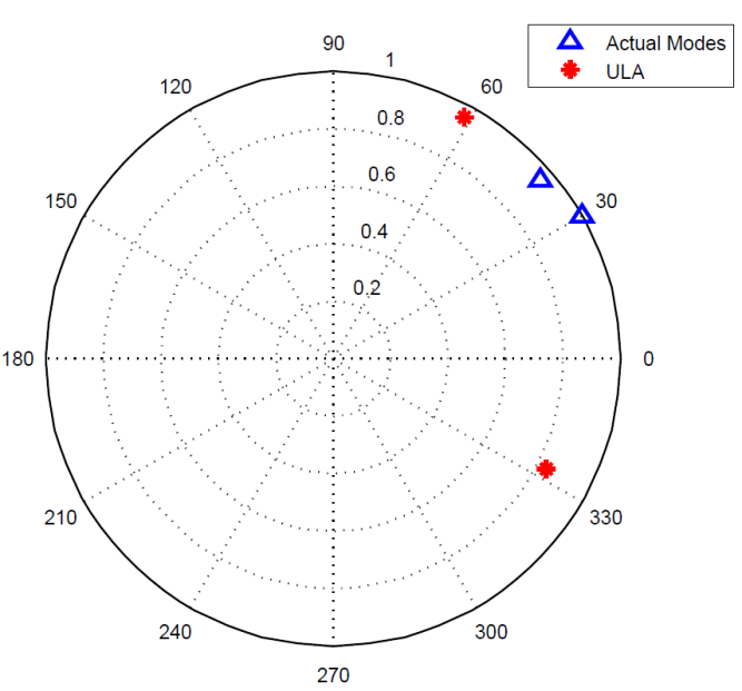
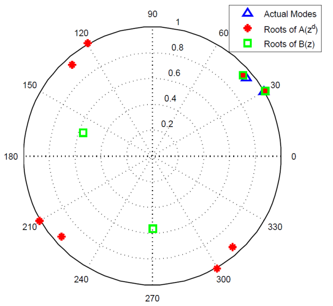
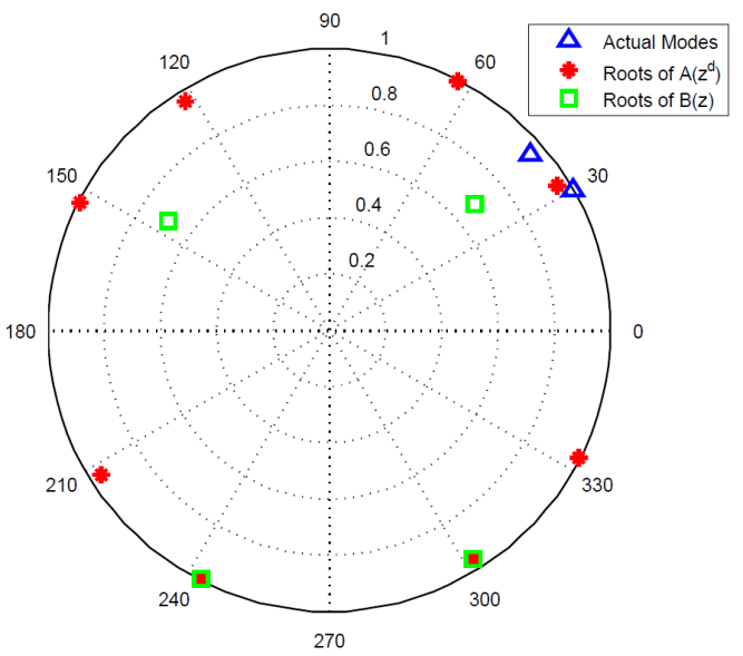
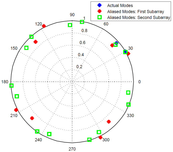
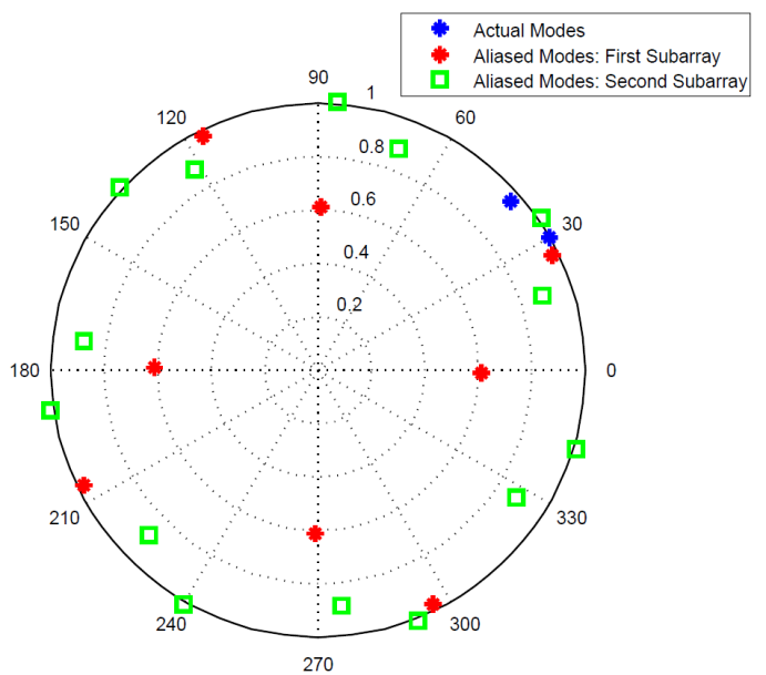
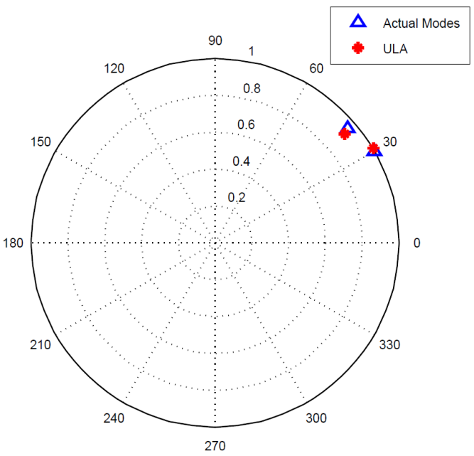
We now consider the performance of the approximate least squares estimation methods, shown in Figs. 4-6. The two modes to be estimated here are z1=ej0.52subscript𝑧1superscript𝑒𝑗0.52z_{1}=e^{j0.52} and z2=0.95ej0.69subscript𝑧20.95superscript𝑒𝑗0.69z_{2}=0.95e^{j0.69}. We choose the per sensor SNR values for the sparse and co-prime arrays to be 555 dB higher than the SNR for the ULA, based on our insight in [22] about the threshold SNR for ULA and co-prime arrays. When SNR is decreased, there comes a point where some of the components of the orthogonal subspace better approximate the measurements than some of the components of the signal subspace. This leads to a performance breakdown in the estimation of the modes. The SNR at which this catastrophic breakdown occurs is called the threshold SNR (see [24] and [22]). For the compression ratio of 50/14501450/14, the threshold SNR for the co-prime and sparse arrays is almost 555 dB more than its value for the ULA, which is a consequence of the subsamplings by these arrays. We emphasize that any compression increases the SNR threshold. The use of a co-prime or sparse array instead of a dense uniform line array is only justified in applications where SNR is high enough for the desired estimation resolution, or when SNR can be built up from temporal snapshots using long observation periods. The latter of course requires the scene to remain stationary over the longer estimation period.
Refer to caption Refer to caption
(a) (b)
Figure 4: Estimating two closely spaced modes z1=ej0.52subscript𝑧1superscript𝑒𝑗0.52z_{1}=e^{j0.52} and z2=0.95ej0.69subscript𝑧20.95superscript𝑒𝑗0.69z_{2}=0.95e^{j0.69} using a ULA with 505050 elements: (a) Per sensor SNR =0absent0=0 dB. (b) Per sensor SNR =5absent5=-5 dB.
Refer to caption Refer to caption
(a) (b)
Figure 5: Estimating two closely spaced modes z1=ej0.52subscript𝑧1superscript𝑒𝑗0.52z_{1}=e^{j0.52} and z2=0.95ej0.69subscript𝑧20.95superscript𝑒𝑗0.69z_{2}=0.95e^{j0.69} using a sparse array with 141414 elements, d=4𝑑4d=4 and M=3𝑀3M=3: (a) Per sensor SNR =5absent5=5 dB (b) Per sensor SNR =0absent0=0 dB.
Refer to caption Refer to caption
(a) (b)
Figure 6: Estimating two closely spaced modes z1=ej0.52subscript𝑧1superscript𝑒𝑗0.52z_{1}=e^{j0.52} and z2=0.95ej0.69subscript𝑧20.95superscript𝑒𝑗0.69z_{2}=0.95e^{j0.69} using a co-prime array with 141414 elements, m1=7subscript𝑚17m_{1}=7 and m2=4subscript𝑚24m_{2}=4: (a) Per sensor SNR =5absent5=5 dB (b) Per sensor SNR =0absent0=0 dB.

Appendix A

Let m>2p𝑚2𝑝m>2p and zidzjdsuperscriptsubscript𝑧𝑖𝑑superscriptsubscript𝑧𝑗𝑑z_{i}^{d}\neq z_{j}^{d} for ij𝑖𝑗i\neq j. Also, let 𝐚=(a1,a2,,ap)T𝐚superscriptsubscript𝑎1subscript𝑎2subscript𝑎𝑝𝑇\mathbf{a}=(a_{1},a_{2},\dots,a_{p})^{T} be the solution to (24). That is,

𝐚=argmin𝜶n=0N1𝐲H[n]𝐏𝐀0(𝜶)𝐲[n],𝐚subscriptargmin𝜶superscriptsubscript𝑛0𝑁1superscript𝐲𝐻delimited-[]𝑛subscript𝐏subscript𝐀0𝜶𝐲delimited-[]𝑛\displaystyle\mathbf{a}=\mathop{\mathrm{argmin}}_{\bm{\alpha}}\sum_{n=0}^{N-1}{\bf y}^{H}[n]\mathbf{P}_{{\bf A}_{0}(\bm{\alpha})}{\bf y}[n], (41)

where 𝐀0(𝜶)subscript𝐀0𝜶{{\bf A}_{0}}(\bm{\alpha}) denotes an 𝐀0subscript𝐀0{\bf A}_{0} of the form (18), with αisubscript𝛼𝑖\alpha_{i}’s replacing aisubscript𝑎𝑖a_{i}’s for i=1,2,,p𝑖12𝑝i=1,2,\ldots,p. We wish to show that in the noiseless case the roots of the polynomial A(z)=1+i=1paizi𝐴𝑧1superscriptsubscript𝑖1𝑝subscript𝑎𝑖superscript𝑧𝑖A(z)=1+\sum_{i=1}^{p}a_{i}z^{-i} are wk=zkdsubscript𝑤𝑘superscriptsubscript𝑧𝑘𝑑w_{k}=z_{k}^{d} for k=1,2,,p𝑘12𝑝k=1,2,\dots,p (the d𝑑dth power of the actual modes).

Without loss of generality we assume that N=1𝑁1N=1. Let 𝐲=𝐲[0]𝐲𝐲delimited-[]0{\bf y}={\bf y}[0]. In the noiseless case, the minimum value of the objective function 𝐲H𝐏𝐀0(𝜶)𝐲superscript𝐲𝐻subscript𝐏subscript𝐀0𝜶𝐲{\bf y}^{H}\mathbf{P}_{{\bf A}_{0}(\bm{\alpha})}{\bf y} is zero, and because 𝐀0H(𝜶)𝐀0(𝜶)superscriptsubscript𝐀0𝐻𝜶subscript𝐀0𝜶{\bf A}_{0}^{H}(\bm{\alpha}){\bf A}_{0}(\bm{\alpha}) is always full rank, for the solution vector 𝐚𝐚\mathbf{a}, we have 𝐀0H(𝐚)𝐲=𝟎superscriptsubscript𝐀0𝐻𝐚𝐲0{\bf A}_{0}^{H}(\mathbf{a}){\bf y}=\mathbf{0}. Now, in the noiseless case, 𝐲=𝐕(𝐳,𝕀s)𝐱𝐲𝐕𝐳subscript𝕀𝑠𝐱{\bf y}={\bf V}({\bf z},\mathbb{I}_{s}){\bf x}, where 𝐕(𝐳,𝕀s)𝐕𝐳subscript𝕀𝑠{\bf V}({\bf z},\mathbb{I}_{s}) is given by (16) and 𝐱=[x1,x2,,xp]T𝐱superscriptsubscript𝑥1subscript𝑥2subscript𝑥𝑝𝑇{\bf x}=[x_{1},x_{2},\ldots,x_{p}]^{T} is the vector of mode weights. Therefore, we have

𝐀0H(𝐚)𝐕(𝐳,𝕀s)𝐱=𝟎,superscriptsubscript𝐀0𝐻𝐚𝐕𝐳subscript𝕀𝑠𝐱0{\bf A}_{0}^{H}(\mathbf{a}){\bf V}({\bf z},\mathbb{I}_{s}){\bf x}=\mathbf{0}, (42)

which we can reorder to get

[111z1dz2dzpdz1(mp1)dz2(mp1)dzp(mp1)d][x1000x2000xp][A(w1)A(w2)A(wp)]=𝟎.matrix111superscriptsubscript𝑧1𝑑superscriptsubscript𝑧2𝑑superscriptsubscript𝑧𝑝𝑑superscriptsubscript𝑧1𝑚𝑝1𝑑superscriptsubscript𝑧2𝑚𝑝1𝑑superscriptsubscript𝑧𝑝𝑚𝑝1𝑑matrixsubscript𝑥1000subscript𝑥2000subscript𝑥𝑝matrix𝐴subscript𝑤1𝐴subscript𝑤2𝐴subscript𝑤𝑝0\begin{bmatrix}1&1&\cdots&1\\ z_{1}^{d}&z_{2}^{d}&\cdots&z_{p}^{d}\\ \vdots&\vdots&\ddots&\vdots\\ z_{1}^{(m-p-1)d}&z_{2}^{(m-p-1)d}&\cdots&z_{p}^{(m-p-1)d}\end{bmatrix}\begin{bmatrix}x_{1}&0&\cdots&0\\ 0&x_{2}&\cdots&0\\ \vdots&\vdots&\ddots&\vdots\\ 0&0&\cdots&x_{p}\end{bmatrix}\begin{bmatrix}A(w_{1})\\ A(w_{2})\\ \vdots\\ A(w_{p})\end{bmatrix}=\mathbf{0}. (43)

Because the matrix on the left hand side of (43) is a full column rank Vandermonde matrix, and the diagonal matrix in the middle is nonsingular (by the assumption of having p𝑝p actual modes), the above equality holds iff

A(wk)=0fork=1,,p.formulae-sequence𝐴subscript𝑤𝑘0for𝑘1𝑝A(w_{k})=0\hskip 8.53581pt\textrm{for}\hskip 5.69054ptk=1,\dots,p. (44)

Appendix B

Let m>2p𝑚2𝑝m>2p and zidzjdsuperscriptsubscript𝑧𝑖𝑑superscriptsubscript𝑧𝑗𝑑z_{i}^{d}\neq z_{j}^{d} for ij𝑖𝑗i\neq j. Also, let 𝜷𝜷\bm{\beta} be the solution to (IV-A) in the noiseless case. Here we use 𝜷𝜷\bm{\beta} instead of 𝐛^^𝐛\hat{\mathbf{b}} for the solution to distinguish noiseless and noisy cases. We show 𝜷𝜷\bm{\beta} solves (21) and therefore resolves aliasing.

Again, without loss of generality, we assume N=1𝑁1N=1. Based on our argument in Appendix A, in the noiseless case we have

={(z1ej2πk1/d,z2ej2πk2/d,,zpej2πkp/d)|0k1,k2,,kpd1},conditional-setsubscript𝑧1superscript𝑒𝑗2𝜋subscript𝑘1𝑑subscript𝑧2superscript𝑒𝑗2𝜋subscript𝑘2𝑑subscript𝑧𝑝superscript𝑒𝑗2𝜋subscript𝑘𝑝𝑑formulae-sequence0subscript𝑘1subscript𝑘2subscript𝑘𝑝𝑑1\mathcal{R}=\{(z_{1}e^{j2\pi k_{1}/d},z_{2}e^{j2\pi k_{2}/d},\cdots,z_{p}e^{j2\pi k_{p}/d})\hskip 5.69054pt|\hskip 5.69054pt0\leq k_{1},k_{2},\dots,k_{p}\leq d-1\}, (45)

where {zi}i=1psuperscriptsubscriptsubscript𝑧𝑖𝑖1𝑝\{z_{i}\}_{i=1}^{p} are the actual modes. In this case (IV-A) can be rewritten as:

𝜷=argmin𝜻|ym1+𝜻T𝐮|2s.t.𝐕pT(𝜼)𝜻=𝜼M,𝜼,formulae-sequence𝜷subscript𝜻superscriptsubscript𝑦𝑚1superscript𝜻𝑇𝐮2stformulae-sequencesuperscriptsubscript𝐕𝑝𝑇𝜼𝜻superscript𝜼direct-productabsent𝑀𝜼\bm{\beta}=\arg\min_{\bm{\zeta}}|y_{m-1}+\bm{\zeta}^{T}\mathbf{u}|^{2}\hskip 14.22636pt\mathrm{s.t.}\hskip 5.69054pt{\bf V}_{p}^{T}(\bm{\eta})\bm{\zeta}=-\bm{\eta}^{\odot M},\hskip 5.69054pt\bm{\eta}\in\mathcal{R}, (46)

where 𝜼=(η1,η2,,ηp)𝜼subscript𝜂1subscript𝜂2subscript𝜂𝑝\bm{\eta}=(\eta_{1},\eta_{2},\ldots,\eta_{p}), 𝜼M=[η1M,η2M,,ηpM]Tsuperscript𝜼direct-productabsent𝑀superscriptsuperscriptsubscript𝜂1𝑀superscriptsubscript𝜂2𝑀superscriptsubscript𝜂𝑝𝑀𝑇\bm{\eta}^{\odot M}=[\eta_{1}^{M},\eta_{2}^{M},\ldots,\eta_{p}^{M}]^{T} and

𝐕p(𝜼)=[111η1dη2dηpdη1(p1)dη2(p1)dηp(p1)d].subscript𝐕𝑝𝜼matrix111superscriptsubscript𝜂1𝑑superscriptsubscript𝜂2𝑑superscriptsubscript𝜂𝑝𝑑superscriptsubscript𝜂1𝑝1𝑑superscriptsubscript𝜂2𝑝1𝑑superscriptsubscript𝜂𝑝𝑝1𝑑{\bf V}_{p}(\bm{\eta})=\begin{bmatrix}1&1&\cdots&1\\ \eta_{1}^{d}&\eta_{2}^{d}&\cdots&\eta_{p}^{d}\\ \vdots&\vdots&\ddots&\vdots\\ \eta_{1}^{(p-1)d}&\eta_{2}^{(p-1)d}&\cdots&\eta_{p}^{(p-1)d}\end{bmatrix}. (47)

In the noiseless case, 𝐮=𝐕p(𝐳)𝐱𝐮subscript𝐕𝑝𝐳𝐱\mathbf{u}={\bf V}_{p}({\bf z}){\bf x}, ym1=i=1pxiziMsubscript𝑦𝑚1superscriptsubscript𝑖1𝑝subscript𝑥𝑖superscriptsubscript𝑧𝑖𝑀y_{m-1}=\sum_{i=1}^{p}x_{i}z_{i}^{M} and 𝐕p(𝜼)=𝐕p(𝐳)subscript𝐕𝑝𝜼subscript𝐕𝑝𝐳{\bf V}_{p}(\bm{\eta})={\bf V}_{p}({\bf z}). Therefore, we have

|ym1+𝜷T𝐮|2superscriptsubscript𝑦𝑚1superscript𝜷𝑇𝐮2\displaystyle|y_{m-1}+\bm{\beta}^{T}\mathbf{u}|^{2} =|i=1pxiziM+𝜷T𝐕p(𝐳)𝐱|absentsuperscriptsubscript𝑖1𝑝subscript𝑥𝑖superscriptsubscript𝑧𝑖𝑀superscript𝜷𝑇subscript𝐕𝑝𝐳𝐱\displaystyle=|\sum_{i=1}^{p}x_{i}z_{i}^{M}+\bm{\beta}^{T}{\bf V}_{p}({\bf z}){\bf x}|
=|i=1pxi(ziMηiM)|0.absentsuperscriptsubscript𝑖1𝑝subscript𝑥𝑖superscriptsubscript𝑧𝑖𝑀superscriptsubscript𝜂𝑖𝑀0\displaystyle=|\sum_{i=1}^{p}x_{i}(z_{i}^{M}-\eta_{i}^{M})|\geq 0. (48)

Now, because 𝜷𝜷\bm{\beta} is the solution to (46), then in the noiseless case |ym1+𝜷T𝐮|2=0superscriptsubscript𝑦𝑚1superscript𝜷𝑇𝐮20|y_{m-1}+\bm{\beta}^{T}\mathbf{u}|^{2}=0 and from (Appendix B) we have 𝜼M=𝐳Msuperscript𝜼direct-productabsent𝑀superscript𝐳direct-productabsent𝑀\bm{\eta}^{\odot M}=\mathbf{z}^{\odot M} almost surely. Therefore,

𝜷𝜷\displaystyle\bm{\beta} =(𝐕PT(𝜼))1𝜼Mabsentsuperscriptsuperscriptsubscript𝐕𝑃𝑇𝜼1superscript𝜼direct-productabsent𝑀\displaystyle=-({\bf V}_{P}^{T}(\bm{\eta}))^{-1}\bm{\eta}^{\odot M}
=(𝐕PT(𝐳))1𝐳Mabsentsuperscriptsuperscriptsubscript𝐕𝑃𝑇𝐳1superscript𝐳direct-productabsent𝑀\displaystyle=-({\bf V}_{P}^{T}({\bf z}))^{-1}{\bf z}^{\odot M}
=𝐛,absent𝐛\displaystyle=\mathbf{b}, (49)

where 𝐛𝐛\mathbf{b} is the solution to (21). ~{}\blacksquare

Appendix C

The Fisher information matrix for the measurement model in (2) may be written as

𝐉(𝐳)=n=1N𝐉n(𝐳),n=0,1,,N1,formulae-sequence𝐉𝐳superscriptsubscript𝑛1𝑁subscript𝐉𝑛𝐳𝑛01𝑁1\mathbf{J}({\bf z})=\sum_{n=1}^{N}\mathbf{J}_{n}({\bf z}),\quad n=0,1,\ldots,N-1, (50)

where 𝐉n(𝐳)subscript𝐉𝑛𝐳\mathbf{J}_{n}({\bf z}) is the Fisher information matrix for the estimation of the modes 𝐳=[z1,z2,,zp]T𝐳superscriptsubscript𝑧1subscript𝑧2subscript𝑧𝑝𝑇\mathbf{z}=[z_{1},z_{2},\cdots,z_{p}]^{T} from 𝐲[n]𝐲delimited-[]𝑛{\bf y}[n] in (2). That is,

𝐉n(𝐳)=1σ2𝐆nH(𝐳)𝐆n(𝐳),subscript𝐉𝑛𝐳1superscript𝜎2superscriptsubscript𝐆𝑛𝐻𝐳subscript𝐆𝑛𝐳\mathbf{J}_{n}({\bf z})=\frac{1}{\sigma^{2}}{\bf G}_{n}^{H}({\bf z}){\bf G}_{n}({\bf z}), (51)

where 𝐆n(𝐳)=[𝐠1[n],𝐠2[n],,𝐠p[n]]subscript𝐆𝑛𝐳subscript𝐠1delimited-[]𝑛subscript𝐠2delimited-[]𝑛subscript𝐠𝑝delimited-[]𝑛{\bf G}_{n}({\bf z})=[\mathbf{g}_{1}[n],\mathbf{g}_{2}[n],\cdots,\mathbf{g}_{p}[n]], and

𝐠l[n]=[i0zli01i1zli11i(m1)zli(m1)1]xl[n]subscript𝐠𝑙delimited-[]𝑛matrixsubscript𝑖0superscriptsubscript𝑧𝑙subscript𝑖01subscript𝑖1superscriptsubscript𝑧𝑙subscript𝑖11subscript𝑖𝑚1superscriptsubscript𝑧𝑙subscript𝑖𝑚11subscript𝑥𝑙delimited-[]𝑛\mathbf{g}_{l}[n]=\begin{bmatrix}i_{0}z_{l}^{i_{0}-1}\\ i_{1}z_{l}^{i_{1}-1}\\ \vdots\\ i_{(m-1)}z_{l}^{i_{(m-1)}-1}\end{bmatrix}x_{l}[n] (52)

is the l𝑙lth sensitivity vector, for 1lp1𝑙𝑝1\leq l\leq p. The CRB for the estimation of the k𝑘kth mode zksubscript𝑧𝑘z_{k} is the k𝑘kth diagonal element of 𝐉1(𝐳)superscript𝐉1𝐳\mathbf{J}^{-1}({\bf z}).

VI Acknowledgment

The authors thank Prof. Chris Peterson for pointing out the minimal, p𝑝p-dimensional, characterization of the orthogonal subspace in (9).

References

  • [1] R. Prony, “Essai expérimental et analytique sur les lois de la dilatabilité des fluides élastiques, et sur celles de la force expansive de la vapeur de l’eau et de la vapeur de l’alkool, á différentes températures,” Journal de L’École Polytechnique (Paris), vol. 1, no. 2, pp. 24–76, 1795.
  • [2] R. Kumaresan, L. L. Scharf, and A. K. Shaw, “An algorithm for pole-zero modeling and spectral analysis,” IEEE Transactions on Acoustics, Speech and Signal Processing, vol. 34, no. 3, pp. 637–640, Jun. 1986.
  • [3] Y. Bresler and A. Macovski, “Exact maximum likelihood parameter estimation of superimposed exponential signals in noise,” IEEE Transactions on Acoustics, Speech and Signal Processing, vol. 34, no. 5, pp. 1081–1089, Oct. 1986.
  • [4] R. Kumaresan and D. W. Tufts, “Estimating the angles of arrival of multiple plane waves,” IEEE Transactions on Aerospace and Electronic Systems, vol. AES-19, no. 1, pp. 134–139, Jan. 1983.
  • [5] R. Kumaresan, D. W. Tufts, and L. L. Scharf, “A Prony method for noisy data: Choosing the signal components and selecting the order in exponential signal models,” Proceedings of the IEEE, vol. 72, no. 2, pp. 230–233, Feb. 1984.
  • [6] R. O. Schmidt, “Multiple emitter location and signal parameter estimation,” IEEE Transactions on Antennas and Propagation, vol. 34, no. 3, pp. 276–280, Mar. 1986.
  • [7] A. Paulraj, R. Roy, and T. Kailath, “Estimation of signal parameters via rotational invariance techniques – ESPRIT,” in Conf. Rec. Nineteeth Asilomar Conference on Circuits, Systems and Computers, Pacific Grove, CA, Nov. 6-8 1985, pp. 83–89.
  • [8] R. Roy and T. Kailath, “ESPRIT – estimation of signal parameters via rotational invariance techniques,” IEEE Transactions on Acoustics, Speech and Signal Processing, vol. 37, no. 7, pp. 984–995, Jul. 1989.
  • [9] F. Belloni, A. Richter, and V. Koivunen, “Extension of root-MUSIC to non-ULA array configurations,” in Proc. IEEE International Conference on Acoustics, Speech and Signal Processing (ICASSP), vol. 4, Toulouse, France, May. 2006, pp. 897–900.
  • [10] M. Rubsamen and A. B. Gershman, “Direction-of-arrival estimation for nonuniform sensor arrays: from manifold separation to fourier domain MUSIC methods,” IEEE Transactions on Signal Processing, vol. 57, no. 2, pp. 588–599, Feb. 2009.
  • [11] B. Friedlander and A. J. Weiss, “Direction finding using spatial smoothing with interpolated arrays,” IEEE Transactions on Aerospace and Electronic Systems, vol. 28, no. 2, pp. 574–587, Apr. 1992.
  • [12] B. Friedlander, “The root-MUSIC algorithm for direction finding with interpolated arrays,” Signal Processing, vol. 30, no. 1, pp. 15–29, Jun. 1993.
  • [13] F. Gao and A. B. Gershman, “A generalized ESPRIT approach to direction-of-arrival estimation,” IEEE signal processing letters, vol. 12, no. 3, pp. 254–257, Mar. 2005.
  • [14] L. Coluccio, A. Eisinberg, and G. Fedele, “A prony-like method for non-uniform sampling,” Signal Processing, vol. 87, no. 10, pp. 2484–2490, Oct. 2007.
  • [15] T. Peter, D. Potts, and M. Tasche, “Nonlinear approximation by sums of exponentials and translates,” SIAM Journal on Scientific Computing, vol. 33, no. 4, pp. 1920–1947, Aug. 2011.
  • [16] A. Moffet, “Minimum-redundancy linear arrays,” IEEE Trans. Antennas and Propagation, vol. 16, no. 2, pp. 172–175, Mar. 1968.
  • [17] P. Pal and P. P. Vaidyanathan, “Coprime sampling and the MUSIC algorithm,” in IEEE Digital Signal Processing Workshop and IEEE Signal Processing Education Workshop (DSP/SPE), Coolum, Queensland, Australia, Jan. 2011, pp. 289–294.
  • [18] P. P. Vaidyanathan and P. Pal, “Sparse sensing with co-prime samplers and arrays,” IEEE Transactions on Signal Processing, vol. 59, no. 2, pp. 573–586, Feb. 2011.
  • [19] ——, “Why does direct-MUSIC on sparse-arrays work?” in Conf. Rec. Asilomar Conference on Signals, Systems and Computers, Pacific Grove, CA, Nov. 2013, pp. 2007–2011.
  • [20] P. Pakrooh, L. L. Scharf, A. Pezeshki, and Y. Chi, “Analysis of Fisher information and the Cramer-Rao bound for nonlinear parameter estimation after compressed sensing,” in Proc. IEEE International Conference on Acoustics, Speech and Signal Processing (ICASSP), Vancouver, BC, Canada, May 2013, pp. 6630–6634.
  • [21] P. Pakrooh, A. Pezeshki, L. L. Scharf, D. Cochran, and S. D. Howard, “Analysis of Fisher information and the Cramér-Rao bound for nonlinear parameter estimation after compressed sensing,” IEEE Transactions on Signal Processing, submitted Feb. 2015.
  • [22] P. Pakrooh, A. Pezeshki, and L. L. Scharf, “Threshold effects in parameter estimation from compressed data,” in Proc. IEEE Global Conference on Signal and Information Processing (GlobalSIP), Austin, Tx, Dec. 2013, pp. 997–1000.
  • [23] J. McClellan and D. Lee, “Exact equivalence of the Steiglitz-McBride iteration and IQML,” IEEE Transactions on Signal Processing, vol. 39, no. 2, pp. 509–512, Feb. 1991.
  • [24] J. K. Thomas, L. L. Scharf, and D. W. Tufts, “The probability of a subspace swap in the SVD,” IEEE Transactions on Signal Processing, vol. 43, no. 3, pp. 730–736, Mar. 1995.