On the $BMAP_{1},BMAP_{2}/PH/g,c$ retrial queueing system

Abstract

In this paper, we analyze a retrial queueing system with Batch Markovian Arrival Processes and two types of customers. The rate of individual repeated attempts from the orbit is modulated according to a Markov Modulated Poisson Process. Using the theory of multi-dimensional asymptotically quasi-Toeplitz Markov chain, we obtain the stability condition and the algorithm for calculating the stationary state distribution of the system. Main performance measures are presented. Furthermore, we investigate some optimization problems. The algorithm for determining the optimal number of guard servers and total servers is elaborated. Finally, this queueing system is applied to the cellular wireless network. Numerical results to illustrate the optimization problems and the impact of retrial on performance measures are provided. We find that the performance measures are mainly affected by the two types of customers’ arrivals and service patterns, but the retrial rate plays a less crucial role.

Keywords: Queueing; Markov Modulated Poisson Process; Asymptotically quasi-Toeplitz Markov chains; Cellular wireless networks; Performance evaluation

1.  Introduction

Most queueing systems assume that the arrival process is a stationary Poisson process. But such a process does not characterize the typical features of traffic in modern telecommunication networks such as correlation and burstiness. The batch Markovian arrival process (BMAP) is a useful and appropriate model for describing such features. The BMAP is a generalization of many well-known processes including the Markovian arrival process (MAP), the Markov-modulated Poisson process (MMPP), the PH-renewal process and the Poisson process. Furthermore, the BMAP preserves the tractable Markovian structure. The origins of the BMAP can be traced to the development of the versatile Markovian point process by Neuts (1979). The currently used denotations were introduced in Neuts (1989). It is widely employed in research for queueing systems, inventory systems, reliability engineering, manufacturing systems, computer communication systems, insurance problems and so on. Chakravarthy (1999) gave a detailed survey of the results about the queues which the input flow is BMAP. Heyman & Lucantoni (2003) presented an application of the BMAP for modeling the information flows in the modern telecommunication networks.

Retrial queues are very good mathematical models for cellular wireless networks, telephone switching systems, local area networks under the protocols of random multiple access, computer systems for competing to gain service from a central processor unit, etc. Over recent years it has been a rapid growth in the literature on retrial queues. The reader can refer to the survey papers by Falin (1990), Artalejo (1990, 2010), Yang & Templeton (1987) for a review of main results and methods. Most of the papers and books are focused on single server retrial queues. Multi-server retrial queues are more complicated for research and even the model M/M/c is studied until now only algorithmically via different truncation schemes. The multi-server retrial queues with the BMAP are still not well investigated in literature. In Breuer et al. (2002), the classical BMAP/PH/N retrial queue was analyzed by means of discrete-time multi-dimensional asymptotically quasi-Toeplitz Markov chain. He et al. (2000) gave the stable condition for the BMAP/PH/S/S+K retrial queue with PH-retrial times. Recently, Klimenok et al. (2007) analyzed the BMAP/PH/N retrial queue with impatient customers. Later, Kim et al. (2008) studied the BMAP/PH/N retrial queue with Markovian flow of breakdowns. Subsequently, Kim et al. (2010) considered the BMAP/PH/N retrial queueing system operating in Markovian random environment. Dudin & Klimenok (2012) investigated the BMAP/PH/N retrial queue with Markov modulated retrials. Particularly, for the retrial queues with two types of customers, the single server retrial queues have received considerable attention in the literature. For example, using the supplementary variable method, Choi & Park (1990) dealt with an $M_{1},M_{2}/G/1$ retrial queue with two types of customers and non-preemptive resume priority. After that, Choi and Park’s model was extended to an $M_{1},M_{2}/G_{1},G_{2}/1$ retrial queue with priority customers by Falin et al. (1993). Later, Choi et al. (1995) investigated an $M/G/1$ retrial queue with two types of customers and finite capacity. Furthermore, using the matrix analytic method, Martin & Artalejo (1995) studied an $M_{1},M_{2}/G_{1},G_{2}/1/1$ retrial queue with impatient customers. In addition, Choi & Chang (1999) presented a survey of single server retrial queue with two types of customers and priority. Recently, Wu & Lian (2013) introduced negative customers into the retrial queues with two types of customers. However, to the best of our knowledge, little work has been done on multi-server retrial queues with two types of customers, and no work on BMAP/PH/N retrial queue with two types of customers is found in the queueing literature.

Our model can be successfully studied by means of asymptotically quasi-Toeplitz Markov chains. Here, we briefly introduce the continuous-time multi-dimensional asymptotically quasi-Toeplitz Markov chains. For a comprehensive and excellent overview of multi-dimensional asymptotically quasi-Toeplitz Markov chains with discrete and continuous time, readers may refer to the paper Klimenok & Dudin (2006). The next definition and propositions follow Klimenok & Dudin (2006). Let $\xi_{t}=\{i_{t},\mathbf{a}_{t}\}$, $t\geq 0$, be a regular irreducible continuous time Markov chain with the state space $\Omega=\{(i,\mathbf{a}),\mathbf{a}\in L_{i},i=0,1,\cdots,i^{0};(i,\mathbf{a}),\mathbf{a}\in L,i>i^{0}\}$. Enumerate the states of the chain $\{\xi_{t}$, $t\geq 0\}$ as follows: the states $(i,\mathbf{a})$ are numerated in ascending order of the component $i$ and for fixed $i$, the states $(i,\mathbf{a})$ are arranged in lexicographic order. We denote the block matrix $Q=(Q_{i,j})$ as the generator of the chain, where the block $Q_{i,j}$ is formed by intensities $q_{(i,\mathbf{a});(j,\mathbf{b})}$ of the chain, transition from the state $(i,\mathbf{a})$ to the state $(j,\mathbf{b})$.

Definition 1.1.

A regular irreducible continuous time Markov chain $\{\xi_{t},t\geq 0\}$ is called asymptotically quasi-Toeplitz Markov chain if

1. $Q_{i,j}=0$ for $j<i-1$, $i>0$.

2. There exit matrices $Y_{n},n\geq 0$, such that

   $$Y_{n} =\lim_{i\to\infty}\Lambda_{i}^{-1}Q_{i,i+n-1},\ \ \ n=0,2,3,\cdots,$$

   $$Y_{1} =\lim_{i\to\infty}\Lambda_{i}^{-1}Q_{i,i}+I,$$

   and the matrix $\sum_{n=0}^{\infty}Y_{n}$ is stochastic.

3. The jump chain $\{\xi_{n},n\geq 1\}$ of the process $\{\xi_{t},t\geq 0\}$ is non-periodic,

where the diagonal matrix $\Lambda_{i}$ defines the diagonal entries of the block $-Q_{ii}$, $i\geq 0$.

Let $Y(z)=\sum_{k=0}^{\infty}Y_{k}z^{k}$ be the matrix generating function characterizing the limiting Markov chain. The following two propositions present the ergodicity conditions for the Markov chain $\{\xi_{t},t\geq 0\}$ in terms of the generating function $Y(z)$ based on whether the matrix $Y(1)$ is an irreducible matrix or not.

Proposition 1.1.

If $Y(1)$ is an irreducible matrix and assume that

1. the series $\sum_{n=1}^{\infty}nQ_{i,i+n-1}\mathbf{e}$ converges for $i=\overline{0,i^{0}}$,

2. the series $\sum_{n=1}^{\infty}nQ_{i,i+n-1}\mathbf{e}$ converges for $i>i^{0}$, and there exists a positive integer $i^{*}>i^{0}$ such that this series converges uniformly in the region $i\geq i^{*}$,

3. the sequence $\Lambda_{i}^{-1}$, $i\geq 0$, has an upper bound,

then the sufficient condition for the Markov chain $\{\xi_{t},t\geq 0\}$ ergodicity is the fulfillment of the inequality

$$\left[\det(zI-Y(z))\right]^{\prime}|_{z=1}>0.$$

If $Y(1)$ is a reducible matrix, then it can be presented in a normal form which has the following structure:

$$Y(z)=\left(\begin{array}[]{ccccc}Y^{(1)}(z)&&&&\\ &Y^{(2)}(z)&&&\\ &&\ddots&&\\ &&&Y^{(l)}(z)&\\ Y^{(l+1,1)}(z)&Y^{(l+1,2)}(z)&\cdots&Y^{(l+1,l)}(z)&Y^{(l+1)}(z)\end{array}\right),$$

where $Y^{(i)}(z)$, $i=\overline{1,l}$, are irreducible square matrices.

Proposition 1.2.

If $Y(1)$ is a reducible matrix of the above form and the conditions of (i)-(iii) of Proposition 1.1 are satisfied, then the sufficient condition for the Markov chain $\{\xi_{t},t\geq 0\}$ ergodicity is the fulfillment of the inequality

$$\left[\det(zI-Y^{(i)}(z))\right]^{\prime}|_{z=1}>0,\ \ \ i=\overline{1,l}.$$

The rest of the paper is organized as follows. The model description is given in Section 2. The Markov chain associated with the system is analyzed in Section 3 where we formulate the model as a multi-dimensional asymptotically quasi-Toeplitz Markov chain and obtain the ergodicity condition of the Markov chain. The algorithms for calculating the stationary state probabilities are elaborated in Section 4. A set of performance measures is demonstrated in Section 5. Two optimization problems and an algorithm for calculating the optimal values are provided in Section 6. An application for the model under discussion and some numerical examples are shown in Section 7. Finally, summary of the results is presented in Conclusion.

2.  Model Description

We consider a multi-server retrial queueing system. Two types of customers (primary customers and priority customers) arrive to the system according to two independent BMAPs (denoted by $BMAP_{1}$ and $BMAP_{2}$). The notion of the BMAP and its detailed description were given by Neuts (1989). We denote the directing process of the $BMAP_{1}$ by $\{\nu_{t},t\geq 0\}$ with the state space $\{1,\cdots,W\}$ and the directing process of the $BMAP_{2}$ by $\{\gamma_{t},t\geq 0\}$ with the state space $\{1,\cdots,V\}$. The two directing processes behave as two independent irreducible continuous-time Markov chains. Denote the matrix sequences $(D_{n}:n\in\mathbb{N}_{0})$ and $(E_{n}:n\in\mathbb{N}_{0})$ as the sequences of characterizing matrices for the $BMAP_{1}$ and $BMAP_{2}$, respectively. Introduce the matrix generating functions $D(z)=\sum_{n=0}^{\infty}D_{n}$ and $E(z)=\sum_{n=0}^{\infty}E_{n}$, $|z|<1$. We assume the matrix functions $D(z)$ and $E(z)$ satisfy all assumptions of Lucantoni (1991). Therefore, the matrix $D(1)$ is the generator of the process $\{\nu_{t},t\geq 0\}$ and the matrix $E(1)$ is the generator of the process $\{\gamma_{t},t\geq 0\}$. Suppose that the two arrival processes $BMAP_{1}$ and $BMAP_{2}$ start with the initial phase probability distributions $\alpha_{1}$ and $\alpha_{2}$, respectively. Let $\theta_{1}$ and $\theta_{2}$ be the stationary probability vectors of $D(1)$ and $E(1)$, respectively. Then $\lambda_{1}=\theta_{1}D^{\prime}(1)\mathbf{e}$ is the stationary arrival rate of the primary customers and $\lambda_{2}=\theta_{2}E^{\prime}(1)\mathbf{e}$ is the stationary arrival rate of the priority customers. Moreover, we define $\lambda_{b1}=\theta_{1}(-D_{0})\mathbf{e}$ and $\lambda_{b2}=\theta_{2}(-E_{0})\mathbf{e}$ as the intensities of group primary arrivals and group priority arrivals, respectively. Here $\mathbf{e}$ is a column vector of appropriate size with all elements equal to 1.

The service facility consists of $c$ ($c\geq 2$) identical servers which are identical and operate independently of each other. All customers have the same independent, identical PH distributed service times $S$ which is governed by the irreducible continuous time Markov chain $\{m_{t},t\geq 0\}$ with the state space $\{1,\cdots,M\}$. The transitions of the Markov chain $\{m_{t},t\geq 0\}$, which do not lead to service completion, are defined by the irreducible matrix $S$ of size $M\times M$. The transitions of the Markov chain $\{m_{t},t\geq 0\}$, which lead to service completion, are defined by the vector $S_{0}=-S\mathbf{e}$. At the service beginning epoch, the state of the process $\{m_{t},t\geq 0\}$, is determined by the probabilistic row vector $\varsigma$ of size $1\times M$. The service time distribution function has the form $B(x)=1-\varsigma e^{Sx}\mathbf{e}$. The mean rate of service is $\mu=[-\varsigma S^{-1}\mathbf{e}]^{-1}$. A more detailed information about the PH type distribution can be seen in the books Neuts (1981), Latouche & Ramaswami (1999) and He (2014).

When a batch of priority customers arrives at the system and there are several servers being idle, the priority customers occupy the corresponding number of the servers. If the number of the idle servers is insufficient (or all the servers are busy) the rest of the batch (or all the batch) enters the retrial group (called orbit). When a batch of primary customers arrives at the system and meets no more than $g-1$ ($1\leq g\leq c-1$) busy servers, the primary customers occupy the corresponding number of the servers (If the number of the idle servers is insufficient, the rest of the batch goes to the orbit); otherwise, the whole batch of primary customers is blocked and goes to the orbit. These customers in orbit are said to be repeated customers and the orbit capacity is assumed to be unlimited. For all customers in the orbit, the individual repeated attempts are governed by a common Markov Modulated Poisson Process (MMPP). The directing process of the Markov Modulated Poisson Process is denoted by $\{r_{t},t\geq 0\}$ which is an irreducible continuous time Markov chain with the state space $\{1,\cdots,R\}$. Transition intensities of the Markov chain $\{r_{t},t\geq 0\}$, which are not related with customers retrials, are defined by the matrix $T_{0}$, and transition intensities, which are accompanied by retrial, are described by the diagonal matrix $T_{1}=\mbox{diag}\{\sigma_{1},\cdots,\sigma_{R}\}$. The matrices $T=T_{0}+T_{1}$ is the infinitesimal generators of the processes $\{r_{t},t\geq 0\}$. That is, when the process $r_{t}$ stays in the state $r$, $r=1,\cdots,R$, each customer from the orbit makes attempts to seek the service at exponentially distributed time intervals with mean $1/\sigma_{r}$. Hence, the total rate of retrials is equal to $n\sigma_{r},\sigma_{r}>0$, when the process $r_{t}$ is in the state $r$ and the orbit size (the number of calls on the orbit) is equal to $n$, $n>0$. Let $\theta_{0}$ be the stationary probability vector of $T$. Then $\sigma=\theta_{0}T_{1}\mathbf{e}$ is the stationary retrial rate of the repeated calls in the orbit. On retrial, an orbiting customer obtains service immediately from one of the idle servers if the number of busy servers is no more than $g-1$; otherwise it will return to the orbit for later retrial. We understand that there are $c-g$ servers (called guard servers) opening only for the priority customers.

For the use in the sequel, let us introduce the following notations:
$\star$ $\mathbf{e}$ is a column vector of ones of suitable size. When needed we will identify the dimension of this vector with a subindex;
$\star$ $I$ is an identity matrix of appropriate size. When needed we will identify the dimension of this matrix with a subindex;
$\star$ $O_{L}$ is a zero matrix of size $L\times L$;
$\star$ $\mbox{\emph{diag}}\{a_{r},r=\overline{1,L}\}$ is a diagonal matrix with diagonal entries $a_{r}$, $r=\overline{1,L}$;
$\star$ $\otimes$ and $\oplus$ are the symbols of Kronecker product and sum of matrices, see, e.g. Graham (1981);
$\star$ $\Omega^{\otimes l}=\underbrace{\Omega\otimes\cdots\otimes\Omega}\limits_{l}$, $l\geq 1$, $\Omega^{\otimes 0}=1,\Omega^{\oplus 0}=0$;
$\star$ $\Omega^{\oplus l}=\sum\limits_{m=0}^{l-1}I_{n^{m}}\otimes\Omega\otimes I_{n^{l-m-1}}$, $l\geq 1$, for the matrix $\Omega$ having $n$ rows.

Our work objectives are to derive the stability condition, to calculate the stationary state distribution, to derive the main performance measures of the system and optimize the values of $g$ and $c$.

3.  Analysis

In this section, we first adopt a layered approach for the description of the state space to construct the infinitesimal generator $\mathbf{Q}$ of the Markov chain which can represent the model. We then derive the ergodicity condition of the Markov chain.

Let
$\ast$ $o_{t}$ be the number of repeated customers in the orbit, at the epoch $t$, $t\geq 0$, $o_{t}\geq 0$;
$\ast$ $b_{t}$ be the number of busy servers, at the epoch $t$, $t\geq 0$, $b_{t}=\overline{0,c}$;
$\ast$ $r_{t}$ be the state of the directing process of the MMPP of repeated customers, at the epoch $t$, $t\geq 0$, $r_{t}=\overline{1,R}$;
$\ast$ $\nu_{t}$ be the state of the directing process of the BMAP of primary customers, at the epoch $t$, $t\geq 0$, $\nu_{t}=\overline{1,W}$;
$\ast$ $\gamma_{t}$ be the state of the directing process of the BMAP of priority customers, at the epoch $t$, $t\geq 0$, $\gamma_{t}=\overline{1,V}$;
$\ast$ $m_{t}^{(j)}$ be the state of the directing process of the service on the $j$th busy server, at the epoch $t$, $t\geq 0$, $m_{t}^{(j)}=\overline{1,M}$, $j=\overline{1,b_{t}}$. Here, we assume that the busy servers are numerated in order of their occupying, i.e., the server, which begins the service, is appointed the maximal number among all busy servers; when some server finishes the service and is released, the servers are correspondingly enumerated.

Then, the process of the model can be described by the regular irreducible continuous time multi-dimensional Markov chain:

$$\xi=\{\xi_{t},t\geq 0\}=\left\{o_{t},b_{t},r_{t},\nu_{t},\gamma_{t},m_{t}^{(1)},\cdots,m_{t}^{(b_{t})},t\geq 0\right\},$$

with the state space

$$\Omega = \left\{\left(o,b,r,\nu,\gamma,m^{(1)},\cdots,m^{(b)}\right);\right.$$

$$\left.o\geq 0,b=\overline{0,c},r=\overline{1,R},\nu=\overline{1,W},\gamma=\overline{1,V},m^{(i)}=\overline{1,M},i=\overline{1,b}\right\},$$

and the dimension of the state space of the Markov chain $\{\xi_{t},t\geq 0\}$ is equal to $K=RWV\frac{1-M^{c+1}}{1-M}$. We note that the dimension $K$ can be very large. E.g., if the array $(c,R,W,V,M)$ is equal to $(10,2,2,2,2)$, then $K=16376$.

We suppose that the states of the Markov chain $\{\xi_{t},t\geq 0\}$ are enumerated in lexicographic order. By means of considering the probabilities of the Markov chain transitions during an infinitesimal time interval, the infinitesimal generator matrix $\mathbf{Q}$ of the Markov chain $\{\xi_{t},t\geq 0\}$ has the following structure:

$$\mathbf{Q}=\left(\begin{array}[]{ccccc}\mathbf{Q}_{00}&\mathbf{Q}_{01}&\mathbf{Q}_{02}&\mathbf{Q}_{03}&\cdots\\ \mathbf{Q}_{10}&\mathbf{Q}_{11}&\mathbf{Q}_{12}&\mathbf{Q}_{13}&\cdots\\ &\mathbf{Q}_{21}&\mathbf{Q}_{22}&\mathbf{Q}_{23}&\cdots\\ &&\mathbf{Q}_{32}&\mathbf{Q}_{33}&\cdots\\ &&&\ddots&\ddots\end{array}\right),$$ (3.6)

where the blocks $\mathbf{Q}_{ij}$ of size $K\times K$ are defined by:

$$(\mathbf{Q}_{i,i})_{l,l^{\prime}}=\left\{\begin{array}[]{ll}O,&l^{\prime}<l-1,l=\overline{2,c},\\ I_{RWV}\otimes S_{0}^{\oplus l},&l^{\prime}=l-1,l=\overline{1,c},\\ T_{0}\oplus D_{0}\oplus E_{0}\oplus S^{\oplus l}-iT_{1}\otimes I_{WVM^{l}},&l^{\prime}=l,l=\overline{0,g-1},\\ T_{0}\oplus D_{0}\oplus E_{0}\oplus S^{\oplus l},&l^{\prime}=l,l=\overline{g,c},\\ I_{R}\otimes(D_{r}\oplus E_{r})\otimes I_{M^{l}}\otimes\varsigma^{\otimes r},&l^{\prime}=l+r,r=\overline{1,g-l},l=\overline{0,g-1},\\ I_{RW}\otimes E_{r}\otimes I_{M^{l}}\otimes\varsigma^{\otimes r},&l^{\prime}=l+r,r=\overline{g+1-l,c-l},l=\overline{0,g-1},\\ I_{RW}\otimes E_{r}\otimes I_{M^{l}}\otimes\varsigma^{\otimes r},&l^{\prime}=l+r,r=\overline{1,c-l},l=\overline{g,c-1}.\end{array}\right.\ \ \ i\geq 0,$$

$$\mathbf{Q}_{i,i-1}=i\bordermatrix{&\scriptstyle 0&\scriptstyle 1&\scriptstyle 2&\cdots&\scriptstyle g&\cdots&\scriptstyle c\cr\scriptstyle 0&&T_{1}\otimes I_{WV}\otimes\varsigma&&&&&\cr\scriptstyle 1&&&T_{1}\otimes I_{WVM}\otimes\varsigma&&&&\cr\vdots&&&&\ddots&&&\cr\scriptstyle g-1&&&&&T_{1}\otimes I_{WVM^{g-1}}\otimes\varsigma&&\cr\scriptstyle g&&&&&&&\cr\vdots&&&&&&&\cr\scriptstyle c&&&&&&&},\ \ \ i\geq 1,$$

$$\mathbf{Q}_{i,i+k}=\bordermatrix{&\scriptstyle 0&\scriptstyle 1&\cdots&\cdots&\scriptstyle g&\cdots&\scriptstyle c-1&\scriptstyle c\cr\scriptstyle 0&&&&&I_{R}\otimes D_{k+g}\otimes I_{V}\otimes\varsigma^{\otimes g}&&&I_{RW}\otimes E_{k+c}\otimes\varsigma^{\otimes c}\cr\scriptstyle 1&&&&&I_{R}\otimes D_{k+g-1}\otimes I_{VM}\otimes\varsigma^{\otimes(g-1)}&&&I_{RW}\otimes E_{k+c-1}\otimes I_{M}\otimes\varsigma^{\otimes(c-1)}\cr\vdots&&&&&\vdots&&&\vdots\cr\scriptstyle g-1&&&&&I_{R}\otimes D_{k+1}\otimes I_{VM^{g-1}}\otimes\varsigma&&&\vdots\cr\scriptstyle g&&&&&I_{R}\otimes D_{k}\otimes I_{VM^{g}}&&&\vdots\cr\vdots&&&&&&\ddots&&\vdots\cr\scriptstyle c-1&&&&&&&I_{R}\otimes D_{k}\otimes I_{VM^{c-1}}&I_{RW}\otimes E_{k+1}\otimes I_{M^{c-1}}\otimes\varsigma\cr\scriptstyle c&&&&&&&&I_{R}\otimes D_{k}\otimes I_{VM^{c}}+I_{RW}\otimes E_{k}\otimes I_{M^{c}}},$$

$i\geq 0$, $k\geq 1$.

Remark 3.1.

When $E_{n}=0$, $n=0,1,\cdots$ and $c=g$, the present system reduces to a retrial BMAP/PH/c queueing system with Markov modulated retrials. It may be noted that the results above after putting $E_{n}=0$, $n=0,1,\cdots$ and $c=g$ agree with the result presented in Dudin & Klimenok (2012).

In the following sections, we analyze the queueing system by using the theory of multi-dimensional asymptotically quasi-Toeplitz Markov chains.

The diagonal blocks of the generator $\mathbf{Q}$ are given by

$$(Q_{ii})_{l,l}=\left\{\begin{array}[]{ll}T_{0}\oplus D_{0}\oplus E_{0}\oplus S^{\oplus l}-iT\otimes I_{WVM^{l}},&l=\overline{0,g-1},\\ T_{0}\oplus D_{0}\oplus E_{0}\oplus S^{\oplus l},&l=\overline{g,c},\end{array}\right.,\ \ \ i\geq 0.$$

Denote the diagonal entries of the matrices $D_{0}$, $E_{0}$ and $S$ as $\{-\lambda^{(1)}_{w},w=\overline{1,W}\}$, $\{-\lambda^{(2)}_{v},v=\overline{1,V}\}$ and $\{-s_{m},m=\overline{1,M}\}$ respectively. Then the diagonal matrix $\Lambda_{i}$ in Definition 1.1 is given by:

$$\Lambda_{i}=\Delta+i\tilde{T}_{1}\hat{I},$$ (3.7)

where

$$\Delta= \mbox{\emph{diag}}\{\mbox{\emph{diag}}\{\sigma_{r},r=\overline{1,R}\}\oplus\mbox{\emph{diag}}\{\lambda^{(1)}_{w},w=\overline{1,W}\}$$

$$\oplus\mbox{\emph{diag}}\{\lambda^{(2)}_{v},v=\overline{1,V}\}\oplus[\mbox{\emph{diag}}\{s_{m},m=\overline{1,M}\}]^{\oplus l},l=\overline{0,c}\},$$

$$\tilde{T}_{1}=\mbox{\emph{diag}}\{T_{1}\otimes I_{WVM^{l}},l=\overline{0,c}\},$$

$$\hat{I}=\left(\begin{array}[]{cc}I_{RWV\sum_{n=0}^{g-1}M^{n}}&\\ &O_{RWV\sum_{n=g}^{c}M^{n}}\end{array}\right).$$

Further, introduce the matrices $\bar{I}$, $\Upsilon$ and $\Gamma_{k}$, $k\geq 0$, of size $K\times K$:

$$\bar{I}=I-\hat{I}=\left(\begin{array}[]{cc}O_{RWV\sum_{n=0}^{g-1}M^{n}}&\\ &I_{RWV\sum_{n=g}^{c}M^{n}}\end{array}\right),$$

$$\Upsilon=\bordermatrix{&\scriptstyle 0&\scriptstyle 1&\scriptstyle 2&\cdots&\scriptstyle g&\cdots&\scriptstyle c\cr\scriptstyle 0&O_{RWV}&I_{RWV}\otimes\varsigma&&&&&\cr\scriptstyle 1&&O_{RWVM}&I_{RWVM}\otimes\varsigma&&&&\cr\vdots&&&\ddots&\ddots&&&\cr\scriptstyle g-1&&&&\ddots&I_{RWVM^{g-1}}\otimes\varsigma&&\cr\scriptstyle g&&&&&O_{RWVM^{g}}&&\cr\vdots&&&&&&\ddots&\cr\scriptstyle c&&&&&&&O_{RWVM^{c}}},$$

$$(\Gamma_{0})_{l,l^{\prime}}=\left\{\begin{array}[]{ll}O,&l^{\prime}<l-1,l=\overline{2,c},\\ I_{RWV}\otimes S_{0}^{\oplus l},&l^{\prime}=l-1,l=\overline{1,c},\\ T_{0}\oplus D_{0}\oplus E_{0}\oplus S^{\oplus l},&l^{\prime}=l,l=\overline{0,c},\\ I_{R}\otimes(D_{r}\oplus E_{r})\otimes I_{M^{l}}\otimes\varsigma^{\otimes r},&l^{\prime}=l+r,r=\overline{1,g-l},l=\overline{0,g-1},\\ I_{RW}\otimes E_{r}\otimes I_{M^{l}}\otimes\varsigma^{\otimes r},&l^{\prime}=l+r,r=\overline{g+1-l,c-l},l=\overline{0,g-1},\\ I_{RW}\otimes E_{r}\otimes I_{M^{l}}\otimes\varsigma^{\otimes r},&l^{\prime}=l+r,r=\overline{1,c-l},l=\overline{g,c-1}.\end{array}\right.$$

$$\Gamma_{k}=Q_{i,i+k},\ \ \ k\geq 1.$$

We obtain:

$$\lim_{i\to\infty}\Lambda_{i}^{-1}=\Delta^{-1}\bar{I},$$ (3.8)

$$Y_{0}=\lim_{i\to\infty}\Lambda_{i}^{-1}Q_{i,i-1}=\Upsilon,$$ (3.9)

$$Y_{1}=\lim_{i\to\infty}\Lambda_{i}^{-1}Q_{ii}+I=\Delta^{-1}\bar{I}\Gamma_{0}+\bar{I},$$ (3.10)

$$Y_{k}=\lim_{i\to\infty}\Lambda_{i}^{-1}Q_{i,i+k-1}=\Delta^{-1}\bar{I}\Gamma_{k-1},\ \ \ k\geq 2,$$ (3.11)

and

$$\sum_{k=0}^{\infty}Y_{k}\mathbf{e}=\mathbf{e}.$$ (3.12)

It can be easily verified that the Markov chain $\{\xi_{t},t\geq 0\}$ satisfies Definition 1.1. Hence, it belongs to the class of asymptotically quasi-Toeplitz Markov chain. From (3.9)-(3.11), we get

$$Y(z)=\Upsilon+\bar{I}z+\Delta^{-1}\bar{I}\Gamma(z)z,\ \ \ |z|<1,$$ (3.13)

where

$$(\Gamma(z))_{l,l^{\prime}} =\left(\sum_{k=0}^{\infty}\Gamma_{k}z^{k}\right)_{l,l^{\prime}}$$

$$=\left\{\begin{array}[]{ll}O,&l^{\prime}<l-1,l=\overline{2,c},\\ I_{RWV}\otimes S_{0}^{\oplus l},&l^{\prime}=l-1,l=\overline{1,c},\\ T_{0}\oplus D_{0}\oplus E_{0}\oplus S^{\oplus l},&l^{\prime}=l,l=\overline{0,g-1},\\ \Xi_{g-l}(z),&l^{\prime}=g,l=\overline{0,g-1},\\ \Theta_{l}(z),&l^{\prime}=l,l=\overline{g,c},\\ I_{R}\otimes(D_{r}\oplus E_{r})\otimes I_{M^{l}}\otimes\varsigma^{\otimes r},&l^{\prime}=l+r,r=\overline{1,g-1-l},l=\overline{0,g-2},\\ I_{RW}\otimes E_{r}\otimes I_{M^{l}}\otimes\varsigma^{\otimes r},&l^{\prime}=l+r,r=\overline{g+1-l,c-1-l},l=\overline{0,g-1},\\ I_{RW}\otimes E_{r}\otimes I_{M^{l}}\otimes\varsigma^{\otimes r},&l^{\prime}=l+r,r=\overline{1,c-1-l},l=\overline{g,c-2},\\ \Psi_{c-l}(z),&l^{\prime}=c,l=\overline{0,c-1},\end{array}\right.$$

here

$$\Xi_{n}(z)=I_{R}\otimes\left[I_{W}\otimes E_{n}+z^{-n}\left(D(z)-\sum_{k=0}^{n-1}D_{k}z^{k}\right)\otimes I_{VM^{g-n}}\right]\otimes\varsigma^{\otimes n},\ \ \ n=\overline{1,g},$$

$$\Theta_{n}(z)=T_{0}\oplus D(z)\oplus E_{0}\oplus S^{\oplus n},\ \ \ n=\overline{g,c-1},$$

$$\Theta_{c}(z)=T_{0}\oplus D(z)\oplus E(z)\oplus S^{\oplus c},$$

$$\Psi_{n}(z)=I_{RW}\otimes z^{-n}\left(E(z)-\sum_{k=0}^{n-1}E_{k}z^{k}\right)\otimes I_{M^{c-n}}\otimes\varsigma^{\otimes n},\ \ \ n=\overline{1,c}.$$

Substituting the expressions of the matrices $\Upsilon$, $\bar{I}$, $\Delta$ and $\Gamma(z)$ in to (3.13), we see that the matrix function $\Gamma(z)$ is of the form

$$Y(z)=\left(\begin{array}[]{cc}Y_{11}&Y_{12}\\ &Y_{22}(z)\end{array}\right),$$ (3.16)

where

$$Y_{11}=\bordermatrix{&\scriptstyle 0&\scriptstyle 1&\scriptstyle 2&\cdots&\scriptstyle g-2\cr\scriptstyle 0&O_{RWV}&I_{RWV}\otimes\varsigma&&&\cr\scriptstyle 1&&\ddots&I_{RWVM}\otimes\varsigma&&\cr\vdots&&&\ddots&\ddots&\cr\scriptstyle g-3&&&&\ddots&I_{RWVM^{g-3}}\otimes\varsigma\cr\scriptstyle g-2&&&&&O_{RWVM^{g-2}}}_{RWV\sum_{i=0}^{g-2}M^{i}},$$

$$Y_{12}=\bordermatrix{&&&&&\cr\scriptstyle 0&&&&&\cr\scriptstyle 1&&&&&\cr\vdots&&&&&\cr\scriptstyle g-2&I_{RWVM^{g-2}}\otimes\varsigma&&&&}_{RWV\sum_{i=0}^{g-2}M^{i}\times RWV\sum_{i=g-1}^{c}M^{i}},$$

$$Y_{22}(z)=\left(\begin{array}[]{cc}O_{RWVM^{g-1}}&Y_{22}^{12}\\ Y_{22}^{21}(z)&Y_{22}^{22}(z)\end{array}\right),$$

$$Y_{22}^{12}=\left(I_{RWVM^{g-1}}\otimes\varsigma,O_{RWVM^{g-1}\times RWV\sum_{n=(g+1)}^{c}M^{n}}\right),$$

$$Y_{22}^{21}(z)=\left(z\Delta_{gg}^{-1}\cdot I_{RWV}\otimes H_{0}^{\oplus g},O_{RWVM^{g-1}\times RWV\sum_{n=(g+1)}^{c}M^{n}}\right)^{T},$$

$$Y_{22}^{22}(z)=z\left(\begin{array}[]{ccccc}\Delta_{gg}^{-1}\Theta_{g}(z)+I&\Delta_{gg}^{-1}\Gamma_{g,g+1}&\cdots&\Delta_{gg}^{-1}\Gamma_{g,c-1}&\Delta_{gg}^{-1}\Psi_{c-g}(z)\\ \Delta_{g+1,g+1}^{-1}\cdot I_{RWV}\otimes H_{0}^{\oplus g+1}&\Delta_{g+1,g+1}^{-1}\Theta_{g+1}(z)+I&\cdots&\Delta_{g+1,g+1}^{-1}\Gamma_{g+1,c-1}&\Delta_{g+1,g+1}^{-1}\Psi_{c-g-1}(z)\\ &\Delta_{g+2,g+2}^{-1}\cdot I_{RWV}\otimes H_{0}^{\oplus g+2}&\cdots&\Delta_{g+2,g+2}^{-1}\Gamma_{g+2,c-1}&\Delta_{g+2,g+2}^{-1}\Psi_{c-g-2}(z)\\ &&\ddots&\vdots&\vdots\\ &&&\Delta_{c-1,c-1}^{-1}\Theta_{c-1}(z)+I&\Delta_{c-1,c-1}^{-1}\Psi_{1}(z)\\ &&&\Delta_{c,c}^{-1}\cdot I_{RWV}\otimes H_{0}^{\oplus c}&\Delta_{c,c}^{-1}\Theta_{c}(z)+I\end{array}\right),$$

here

$$\Delta_{l,l}= \mbox{\emph{diag}}\{\sigma_{r},r=\overline{1,R}\}\oplus\mbox{\emph{diag}}\{\lambda^{(1)}_{w},w=\overline{1,W}\}$$

$$\oplus\mbox{\emph{diag}}\{\lambda^{(2)}_{v},v=\overline{1,V}\}\oplus[\mbox{\emph{diag}}\{s_{m},m=\overline{1,M}\}]^{\oplus l},\ \ \ l=\overline{g,c},$$

$$\Gamma_{l,l^{\prime}}=I_{RW}\otimes E_{r}\otimes I_{M^{l}}\otimes\varsigma^{\otimes r},\ \ \ l^{\prime}=l+r,r=\overline{1,c-1-l},l=\overline{g,c-2}.$$

It is seen from (3.16) that the matrix $Y(z)$ is reducible and the matrix $Y(1)$ contains only one irreducible stochastic diagonal block $Y_{22}(1)$. According to the Proposition 1.2, we get a sufficient condition for ergodicity of the Markov chain $\{\xi_{t},t\geq 0\}$ which is the fulfillment of the following inequality:

$$\left[\det(zI-Y_{22}(z))\right]^{\prime}|_{z=1}>0.$$ (3.17)

A more constructive form of ergodicity condition (3.17) in our system is given by the following theorem.

Theorem 3.1.

A sufficient condition for ergodicity of the Markov chain $\{\xi_{t},t\geq 0\}$, is the fulfillment of the inequality

$$\frac{\lambda_{1}}{\bar{\mu}_{1}}+\frac{\lambda_{2}}{\bar{\mu}_{2}}<1,$$

where

$$\bar{\mu}_{1}=\mathbf{X}_{1}S_{0}^{\oplus g}\mathbf{e}_{M^{g-1}},\ \ \ \bar{\mu}_{2}=\mathbf{X}_{2}S_{0}^{\oplus c}\mathbf{e}_{M^{c-1}},$$

and $\mathbf{X}_{i}$, $i=1,2$, are the unique solutions of the following system of linear algebraic equations:

$$\left\{\begin{array}[]{l}\mathbf{X}_{1}[S^{\oplus g}+S_{0}^{\oplus g}(I_{M^{g-1}}\otimes\varsigma)]=0,\\ \mathbf{X}_{1}\mathbf{e}=1,\end{array}\right.$$

$$\left\{\begin{array}[]{l}\mathbf{X}_{2}[S^{\oplus c}+S_{0}^{\oplus c}(I_{M^{c-1}}\otimes\varsigma)]=0,\\ \mathbf{X}_{2}\mathbf{e}=1.\end{array}\right.$$

Proof. The proof of this theorem follows the steps given in the paper Breuer et al. (2002) and consequently we omit the details here.

Next, we assume that the stability condition is fulfilled. Denote the steady state probabilities of the Markov chain as

$$P\left(o,b,\nu,\gamma,m^{(1)},\cdots,m^{(b)}\right)$$

$$=\lim_{t\to\infty}P\left\{o_{t}=o,b_{t}=b,\nu_{t}=\nu,\gamma_{t}=\gamma,m_{t}^{(1)}=m^{(1)},\cdots,m_{t}^{(b_{t})}=m^{(b)}\right\}.$$

Let the row-vector $\mathbf{P}_{i}$ of dimension $K$ denote the stationary-state probabilities

$$\mathbf{P}_{i}=P\left(i,b,\nu,\gamma,m^{(1)},\cdots,m^{(b)}\right),\ \ \ i\geq 0,$$

and define the infinite-dimensional probability vector $\mathbf{P}=(\mathbf{P}_{1},\mathbf{P}_{2},\cdots)$. When the system is stable, $\mathbf{P}$ is the unique solution to $\mathbf{P}\mathbf{Q}=0$ and $\mathbf{P}\mathbf{e}=1$. However, it is still an open problem to express $\mathbf{P}$ in the closed form (e.g., generating function), and even though $\mathbf{Q}$ is highly structured, $\mathbf{P}$ cannot be expressed in a tractable analytical form. In the following, we will adopt the algorithm of asymptotically quasi-Toeplitz Markov chains to solve the equilibrium equation $\mathbf{P}\mathbf{Q}=0$.

4.  Algorithm

In this section, we use the numerically stable algorithm which has been elaborated in Klimenok & Dudin (2006) to calculate the stationary distribution of the system. The algorithm is based on censoring technique of the asymptotically quasi-Toeplitz Markov chain and consists of some essential steps which are given in the following Algorithm 4.1.

Algorithm 4.1.

Computing the probability vectors $\mathbf{P}_{i}$:
Step 1: Calculate the matrix $G$ as the minimal nonnegative solution to the non-linear matrix equation:

$$G=Y(G).$$ (4.1)

We should note that the first $RWV\frac{1-M^{g}}{1-M}$ rows of the matrix $G$ coincide with corresponding rows of the the matrix $Y(1)$ and the rest $RWV\sum_{n=g}^{c}M^{n}$ entries of the matrix $G$ can be calculated by the iterative method which is available in Lucantoni (1991).
Step 2: Chose the integer $k_{0}$ as a minimal value of $k$ for which the norm $\|G-\sum_{n=k}^{\infty}Q_{k+1,n}G^{n-k}\|$ of the residual is less than the preassigned value $\epsilon$.
Step 3: Calculate the matrices $G_{k_{0}-1}$, $G_{k_{0}-2}$ , $\cdots$, $G_{0}$ from the following recursive equation

$$G_{k}=\left(-\sum_{j=k+1}^{\infty}Q_{k+1,n}G_{j-1}G_{j-2}\cdots G_{k+1}\right)^{-1}Q_{k+1,k},$$ (4.2)

$k=0,1,\cdots,k_{0}-1$, with the boundary condition $G_{k}=G$, $k\geq k_{0}$.
Step 4: Calculate the matrices $\bar{H}_{i,j}$, $j\geq i$, $i\geq 0$,using the formulae

$$\bar{H}_{i,j}=H_{i,j}+\sum_{k=j+1}^{\infty}H_{i,k}G_{k-1}G_{k-2}\cdots G_{j},\ \ \ j\geq i,\ \ \ i\geq 0,$$ (4.3)

where $G_{k}=G$, $k\geq k_{0}$.
Step 5: Calculate the matrices $F_{j}$, $j\geq 0$, according to the recursive relation

$$F_{0}=I,\ \ \ F_{j}=\sum_{i=0}^{j-1}F_{i}\bar{H}_{i,j}(-\bar{H}_{j,j})^{-1},\ \ \ j\geq 1.$$ (4.4)

Step 6: Calculate the vector $\mathbf{P}_{0}$ as the unique solution to the system of the linear equations

$$\left\{\begin{array}[]{l}\mathbf{P}_{0}(-\bar{H}_{0,0})=\mathbf{0},\\ \mathbf{P}_{0}\sum\limits_{j=0}^{\infty}F_{j}\mathbf{e}=1.\end{array}\right.$$

Step 7: Calculate the vectors $\mathbf{P}_{j}$, $j\geq 1$, as

$$\mathbf{P}_{j}=\mathbf{P}_{0}F_{j},\ \ \ j\geq 1.$$

Remark 4.1.

We can eliminate the infinite sums in Step 6 as the following method: pick $N>k_{0}$, and replace the second equation in Step 6 with $\mathbf{P}_{0}\sum\limits_{j=0}^{N}F_{j}\mathbf{e}=1$, such that the inequality $\mathbf{P}_{N}\mathbf{e}<\epsilon_{0}$ is satisfied, where $\epsilon_{0}$ is some preassigned small number. Note that the inverse matrices that appear in the algorithm exist and are nonnegative. So the computation of the algorithm is stable. The algorithm can be realized in framework of extension of “SIRIUS++” software Dudin et al. (2002) that was developed using the results of the asymptotically quasi-Toeplitz Markov chains. As such the determination of the stationary distribution is straightforward.

5.  performance measures

Having the stationary distribution $\mathbf{P}_{i},i\geq 0$ been calculated, we are able to calculate some stationary performance measures of the system under consideration in this section.
Let $\mathbf{P}_{i}=(\mathbf{P}_{i0},\mathbf{P}_{i1},\cdots,\mathbf{P}_{ic})$, $i\geq 0$, where $\mathbf{P}_{ib}$ of size $1\times RWVM^{b}$ is a row vector, $0\leq b\leq c$. Denote $P(i,b)$ the joint probability to have $i$ repeated customers in the orbit and $b$ customers on the servers at arbitrary time. From the results of the above section, we get

$$P(i,b)=\mathbf{P}_{ib}\mathbf{e} =\sum_{r=1}^{R}\sum_{\nu=1}^{W}\sum_{\gamma=1}^{V}\sum_{m^{(1)}=1}^{M}\cdots\sum_{m^{(b)}=1}^{M}P\left(i,b,r,\nu,\gamma,m^{(1)},\cdots,m^{(b)}\right)$$

$$=\mathbf{P}_{i}\mathbf{e}\left[WV\frac{1-M^{b}}{1-M}+1,WV\frac{1-M^{b+1}}{1-M}\right],$$

where $\mathbf{e}\left[RWV\frac{1-M^{b}}{1-M}+1,RWV\frac{1-M^{b+1}}{1-M}\right]$ of size $K\times 1$ is a column vector of suitable size having ones as its $RWV\frac{1-M^{b}}{1-M}+1$th to $RWV\frac{1-M^{b+1}}{1-M}$th entries and zeros as the rest entries.

Corollary 5.1.

1. The probability that there are $i$ repeated customers in the orbit at arbitrary time

   $$P(i,\bullet)=\sum\limits_{b=0}^{c}P(i,b)=\mathbf{P}_{i}\mathbf{e},\ \ \ i\geq 0.$$

2. The probability that there are $b$ busy servers at arbitrary time

   $$P(\bullet,b)=\sum\limits_{i=0}^{\infty}P(i,b),\ \ \ b=\overline{0,c}.$$

3. The mean number of busy servers

   $$L_{b}=\sum\limits_{b=1}^{c}bP(\bullet,b).$$

4. The mean number of repeated customers in the orbit

   $$L_{orb}=\sum\limits_{i=1}^{\infty}i\mathbf{P}_{i}\mathbf{e}.$$

5. The mean number of customers (primary customers and priority customers) in the system

   $$L_{s}=L_{orb}+L_{b}.$$

6. The blocking probability for an arbitrary primary customer

   $$P_{b1}=1-\frac{1}{\lambda_{1}}\sum_{n=1}^{g}\sum_{i=0}^{\infty}P(i,g-n)\sum_{k=0}^{n}(k-n)(I_{R}\otimes D_{k}\otimes I_{VM^{g-n}})\mathbf{e}.$$

7. The blocking probability for an arbitrary batch of primary customers

   $$P_{bb1}=1-\frac{1}{\lambda_{b1}}\sum_{n=1}^{g}\sum_{i=0}^{\infty}P(i,g-n)\sum_{k=1}^{n}(I_{R}\otimes D_{k}\otimes I_{VM^{g-n}})\mathbf{e}.$$

8. The blocking probability for an arbitrary priority customer

   $$P_{b2}=1-\frac{1}{\lambda_{2}}\sum_{n=1}^{c}\sum_{i=0}^{\infty}P(i,c-n)\sum_{k=0}^{n}(k-n)(I_{RW}\otimes E_{k}\otimes I_{M^{c-n}})\mathbf{e}.$$

9. The blocking probability for an arbitrary batch of priority customer

   $$P_{bb2}=1-\frac{1}{\lambda_{b2}}\sum_{n=1}^{c}\sum_{i=0}^{\infty}P(i,c-n)\sum_{k=1}^{n}(I_{RW}\otimes E_{k}\otimes I_{M^{c-n}})\mathbf{e}.$$

10. Busy period: If we define the busy period $B$ of this queueing system with repeated customers as the period that starts at the epoch when an arriving batch of customers (primary or priority) finds an empty system (all servers are idle and no repeated customer in the orbit) and ends at the departure epoch at which the system is empty again, then the mean busy period is given by

    $$E(B)=\frac{1}{\lambda_{1}+\lambda_{2}}\left(\frac{1}{P(0,0)}-1\right).$$

Moreover, using the approach based on Markov renewal processes, we can obtain the following statement.

Proposition 5.1.

The generating function $\Pi(z)$ of the queue state stationary distribution at the departure epochs is characterized by the following functional-differential equation:

$$\Pi^{\prime}(z)=\Pi(z)A(z),$$

where

$$A(z)=B^{-1}(z)B^{\prime}(z)-B^{-1}(z)\Delta(T_{1}^{-1}\otimes I_{WV\sum_{k=0}^{c}M^{k}})z^{-1}B(z)+z^{-1}(T_{1}^{-1}\otimes I_{WV\sum_{k=0}^{c}M^{k}})B(z),$$

$$B(z)=[\Upsilon-z\hat{I}-\Delta^{-1}\hat{I}z\Gamma(z)][\Upsilon-z\hat{I}-\Delta^{-1}\bar{I}z\Gamma(z)]^{-1}.$$

Proof. The proof can be implemented similarly as the proof of Breuer et al. (2002) and is omitted here.

6.  Optimization

In this section, we borrow some ideas and methods from Trivedi et al. (2000) to investigate the optimization problem that how to choose the optimal values of $g$ and $c$ so as to minimize the priority customer blocking probability as well as the primary customer blocking probability. Therefore, we obtain a multi-objective optimization problem in which the number of total servers $c$ and the parameter $g$ which is equal to the number of non-guard servers are the decision variables. However, due to the complexity, we may fix $c$ and only consider $g$ as the decision variable to simply the optimization problem. In the case of the two objectives, we can choose either $P_{b1}$ or $P_{b2}$ as the objective function to be minimized and impose a constraint on the other one. If we regard the two blocking probabilities as two binary functions of $g$ and $c$ two variables, then we write two representative optimization problems as follows:

1. Given $T_{k},D_{k},E_{k},k=0,1,\cdots,S$ and $c$ determine the optimal integer values of $g$ such that

   $$\mbox{Mininize}\ \ \ P_{b1}(g)$$

   $$\mbox{subject to}\ \ \ P_{b2}(g)\leq p_{0}.$$

2. Given $T_{k},D_{k},E_{k},k=0,1,\cdots,S$ determine the optimal integer values of $g$ and $c$ such that

   $$\mbox{Mininize}\ \ \ c$$

   $$\mbox{subject to}\ \ \ P_{b1}(g,c)\leq p_{1},\ \ \ \mbox{and}\ \ \ P_{b2}(g,c)\leq p_{2}.$$

Here, the constants $p_{0}$, $p_{1}$ and $p_{2}$ are three preassigned numbers.

We first consider the optimization problem (I). It is clear that $P_{b2}(g)>P_{b2}(g-1)$ (see Fig. 3). Thus, we can get the largest value of $g$ such that $P_{b2}(g)\leq p_{0}$. Then based on the monotonicity property $P_{b1}(g)>P_{b1}(g+1)$, we know that such a value of $g$ will minimize $P_{b1}(g)$. Therefore, we can obtain the optimal value of $g$ using a simple one dimensional search over the range $\{1,\cdots,c-1\}$ for $g$ such that $g^{*}=\max\{g|P_{b2}(g)\leq p_{0}\}$.

Then we study the optimization problem (II). Since we cannot derive the analytical solution of this system, in the next section, we will resort to the numerical examples to illustrate the optimization problem (II). Here, we provide an algorithm to obtain the minimum value of $c$.

Algorithm 6.1.

Solving the optimization problem (II)
Step 1: Set the values $p_{1}$ and $p_{2}$ and let c=2;
Step 2: For $g=1$ to $c-1$, find the feasible region for $g$:

$$\Theta=\{g|P_{b1}(g,c)\leq p_{1},\ \ \ \mbox{and}\ \ \ P_{b2}(g,c)\leq p_{2}\};$$

Step 3: If $\Theta\neq\emptyset$, then stop and obtain $c^{*}=c$. Otherwise, put $c=c+1$ and goto step 2;
Step 4: Obtain $c^{*}=c$.

7.  Application to cellular wireless networks and numerical examples

In this section, we present an application to cellular wireless networks for the model under discussion and some numerical results that show the effect of the system parameters on the performance measures and channel allocation schemes in the cellular mobile networks. In the cellular mobile wireless network, the regional service area is divided into multiple adjacent cells, each of them served by a base station (BS) with a limited number of channels. Here, we assume the number of channels is equal to $c$, $c\geq 2$. A mobile subscriber who has wireless terminal such as mobile phone for voice service, wireless data terminal for data service, dual terminal for voice and data, and so on, communicates via radio links to a BS, one for each cell. Generally, there are two types of calls in a specific cell in the cellular mobile networks: originating calls, i.e., calls originating in that cell, and handoff calls, i.e., current ongoing calls caused by mobile users moving from one cell to that cell. We assume that the originating calls arrive at the system according to a BMAP with the characterizing matrix sequence $(D_{n}:n\in\mathbb{N}_{0})$ and the handoff calls arrive at the system according to a BMAP with the characterizing matrix sequence $(E_{n}:n\in\mathbb{N}_{0})$. When a batch of new calls originates in that cell, some idle channels are required to the BS for the new calls setup. If there are idle channels in the BS of that cell, then the BS assigns some idle channels to the originating calls; otherwise some new calls (maybe all the batch) in that batch are blocked and the blocked mobile subscribers may try their luck later. Similarly, if some idle channels are available in the BS of that cell, the batch of handoff calls is successfully handed over without an interruption; otherwise some handoff calls (or all the batch) are blocked and retry for service after a short period. Any blocked call (originating or handoff) retries for service where the rates of the retrials depend on a changing environment. Thus, we use the MMPP with the characterizing matrices $(T_{0},T_{1})$ to model the retrial process. The quality of service is disturbed seriously if a handoff call becomes blocked when it crosses the cell boundary. Generally, the base station gives priority to a handoff call over an originating call. The usual way to do this is the scheme with guard channels, see Guerin (1988) and Hong & Rappaport (1996). Here, we assume the number of non-guard channels is equal to $g$. Thus, the number of guard channels is equal to $c-g$. Furthermore, we suppose the conversation time of an ongoing call (originating or handoff) by a channel is of PH type with a representation $(\varsigma,S)$. Then the cellular mobile wireless network can be modeled as a $BMAP_{1},BMAP_{2}/PH/g,c$ retrial queueing system where the rate of individual repeated attempts from the orbit is modulated according to a MMPP. The originating calls can be regarded as primary customers and the handoff calls can be regarded as priority customers.

In the following, we give some simple numerical examples that illustrate the effects of various parameters on the system performance measures of the cellular mobile wireless network. The algorithms 4.1 and 6.1 developed in sections 4 and 6 have been written into some MATLAB programs. Realization of these algorithms on computer does not meet any difficulty. Only the calculation time can be long especially when the dimension of the system is large. For example, if we let $c=8$, then the dimension $K=4088$, and the calculation time is 98s. For $c=100$, the dimension is equal to 1.0141e+031, and the calculation time is very long. Thus, the calculation time increases drastically with the increase of the number of servers $c$. Note that in all the below examples, we choose the parametric values in a way such that the system is stable. Numerical results are showed in Tabs. 1-3 and Figs. 1-3. For comparison, in each of the pictures, we also plot three curves which correspond to $\sigma=6.6429$, $13.2857$ and $26.5714$.

For the convenience of the numerical calculation, here, we suppose that handoff calls and originating calls arrive to the system according to two independent special BMAPs (In fact, they are MAPs) which are characterized by the following matrices:

$$D_{0}=\lambda_{o}\left(\begin{array}[]{cc}-11&2\\ 5&-20\end{array}\right),\ D_{1}=\lambda_{o}\left(\begin{array}[]{cc}8&1\\ 3&12\end{array}\right),\ D_{k}=O_{2},\ k\geq 2,$$

$$E_{0}=\lambda_{h}\left(\begin{array}[]{cc}-3&0\\ 1&-2\end{array}\right),\ E_{1}=\lambda_{h}\left(\begin{array}[]{cc}1&2\\ 0&1\end{array}\right),\ E_{k}=O_{2},\ k\geq 2,$$

This means the stationary arrival rates of the originating calls and the handoff calls are $\lambda_{1}=10.6364\lambda_{o}$ and $\lambda_{2}=1.6667\lambda_{h}$, respectively.

The repeated calls in the orbit repeat there attempts to reach a server according to the MMPP which is defined by the matrices:

$$T_{0}=\lambda_{r}\left(\begin{array}[]{cc}-15&3\\ 4&-19\end{array}\right),\ \ \ T_{1}=\lambda_{r}\left(\begin{array}[]{cc}12&0\\ 0&15\end{array}\right),$$

Thus, the mean retrial rate for the mobile engaged in the cell is $\sigma=13.2857\lambda_{r}$.

The PH service process is defined by the matrices:

$$S=\left(\begin{array}[]{cc}-23&9\\ 14&-17\end{array}\right),\ \ \ \varsigma=(0.4,0.6).$$

So that the mean rate of service is $\mu=8.1288$.

From the above descriptions, we have $W=2,V=2,M=2$ and $R=2$.

Tab. 1: The stationary join distribution of the system with $(c,g,\lambda_{o},\lambda_{h},\lambda_{r})=(8,6,2,2,2)$

$i$ $\backslash$ $b$	0	1	2	3	4	5	6	7	8	$sum$
0	0.0467	0.1413	0.2136	0.2148	0.1604	0.0923	0.0376	0.0016	0.0001	0.9084
1	0.0001	0.0006	0.0020	0.0047	0.0091	0.0149	0.0208	0.0013	0.0001	0.0536
2	0.0000	0.0000	0.0002	0.0008	0.0023	0.0054	0.0109	0.0008	0.0000	0.0206
3	0.0000	0.0000	0.0000	0.0002	0.0007	0.0022	0.0055	0.0005	0.0000	0.0092
4	0.0000	0.0000	0.0000	0.0001	0.0002	0.0009	0.0028	0.0003	0.0000	0.0043
5	0.0000	0.0000	0.0000	0.0000	0.0001	0.0004	0.0014	0.0001	0.0000	0.0020
	1.0e-003 $\times$
6	0.0000	0.0001	0.0007	0.0055	0.0334	0.1661	0.6986	0.0667	0.0051	0.9761
	1.0e-003 $\times$
7	0.0000	0.0000	0.0002	0.0019	0.0130	0.0731	0.3474	0.0337	0.0027	0.4721
	1.0e-003$\times$
8	0.0000	0.0000	0.0001	0.0007	0.0052	0.0325	0.1724	0.0169	0.0014	0.2291
	1.0e-004$\times$
9	0.0000	0.0000	0.0002	0.0025	0.0211	0.1460	0.8533	0.0846	0.0069	1.1145
	1.0e-004$\times$
10	0.0000	0.0000	0.0001	0.0009	0.0087	0.0660	0.4217	0.0421	0.0035	0.5429
$sum$	0.0468	0.1419	0.2158	0.2206	0.1728	0.1162	0.0800	0.0047	0.0002	0.999

Tab. 2: The the optimal value $g^{*}$ for the optimization problem (I) with $(c,\lambda_{o},p_{0})=(20,10,0.0001)$

$\lambda_{r}$ $\backslash$ $\lambda_{h}$	1	2	3	4	5	6	7	8	9	10	11	12	13	14	15	20
1	18	18	18	17	17	17	16	16	16	16	15	15	15	14	14	13
10	18	18	18	17	17	17	16	16	16	16	15	15	15	14	14	13
20	18	18	18	17	17	17	16	16	16	16	15	15	15	14	14	13

Tab. 3: The optimal value $c^{*}$ for the optimization problem (II) with $(\lambda_{r},p_{1},p_{2})=(10,0.001,0.0001)$

$\lambda_{h}$ $\backslash$ $\lambda_{o}$	1	2	3	4	5	6	7	8	9	10	11	12	13	14	15	20
1	8	11	14	16	18	20	22	24	26	28	29	31	33	35	37	45
5	10	13	15	17	19	21	23	25	27	29	30	32	34	36	38	46
10	13	15	17	19	21	23	25	27	29	31	32	34	36	37	39	47

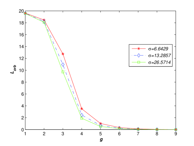
Fig. 1: $L_{orb}$ as function of the parameter $g$ with $(c,\lambda_{o},\lambda_{h})=(10,2,2)$.

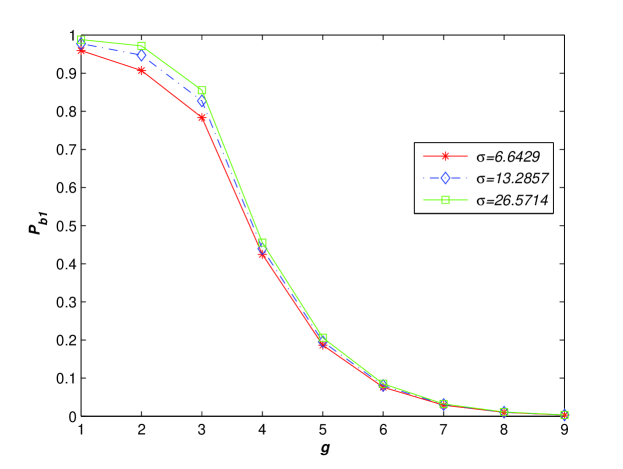
Fig. 2: Dependence of the blocking probability for originating calls on the value $g$ with $(c,\lambda_{o},\lambda_{h})=(10,2,2)$.

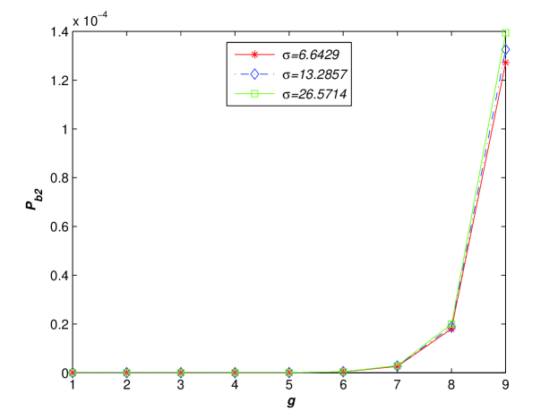
Fig. 3: Dependence of the blocking probability for handoff calls on the value $g$ with $(c,\lambda_{o},\lambda_{h})=(10,2,2)$.

The joint distribution of the number of busy channels and the number of repeated calls in the orbit is presented in Tab. 1 with $(c,g,\lambda_{o},\lambda_{h})=(8,6,2,2)$. From Tab. 1, we observe that the joint probability that there are three busy channels and zero repeated call at arbitrary time is equal to 0.2148 which is the maximum value and the probability that there is no repeated call in the orbit is equal to 0.9084 which is the maximum value of the marginal probabilities (lateral). The probability that there are three busy channels at arbitrary time is equal to 0.2206 which is the maximum value of the marginal probabilities (longitudinal).

The effects of the retrial rate and the arrival rate of the originating calls on the optimal value of $g$ for the optimization problem (I) with the set of parameters $(c,\lambda_{h},\theta_{0})=(20,10,0.0001)$ are reported in Tab. 2. We observe that the optimal value $g^{*}$ decreases monotonously as the arrival rate of the handoff calls increases. From this, we can predict that the optimal value $g^{*}$ increases monotonously as the arrival rate of the originating calls increases. However, the retrial rate of the repeated calls in the orbit has no significant impact on the optimal value $g^{*}$. The appearance of this phenomenon may be based on the fact that the mean number of repeated calls is very small compared to the mean number of arriving calls. Hence it may be concluded that the arrival rates of the two types of calls are the major factors in deciding the optimal numbers of guard channels.

Tab. 3 shows the effects of the arrival rates of the originating calls and the handoff calls on the optimal value $c^{*}$ for the optimization problem (II), where we set $(\lambda_{r},p_{1},p_{2})=(10,0.001,0.0001)$. As is to be expected, when the arrival rates of the two types of calls increase, the optimal value $c^{*}$ increases. Moreover, we observe that the optimal value $c^{*}$ increases faster with the arrival rates of the originating calls than that with the arrival rates of the handoff calls. Therefore, we understand that the arrival of originating calls plays a most significant role in deciding the optimal value $c^{*}$. In other word, this type of calls whose arrival rate is largest will most strongly affect the optimal design of the system.

Fig. 1 illustrates the dependence of the mean number of repeated calls in the orbit on the value of parameter $g$ where we set $(c,\lambda_{o},\lambda_{h})=(10,2,2)$. As it can be seen from Fig. 1 that $L_{orb}$ decreases monotonously as the value $g$ increases, especially when $g\leq 6$. But when $g\geq 7$, the curves of the values $L_{orb}$ are almost overlapping with $x$-axis. That is to say, there are very few repeated customers in the orbit when the number of guard channels is small.

Figs. 2 and 3 show the dependence of the blocking probability for an arbitrary originating call and handoff call on the value of parameter $g$ respectively when $(c,\lambda_{o},\lambda_{h})=(10,2,2)$. From Figs. 2 and 3, we find that the blocking probability for an arbitrary originating call $P_{b1}$ decreases monotonously, but the blocking probability for an arbitrary handoff call $P_{b2}$ increases monotonously as the value $g$ increases, which agrees with the intuitive expectations. In addition, when $g\leq 6$, the curves of the values $P_{b2}$ are almost overlapping with $x$-axis. It means that the blocking probability for an arbitrary handoff call $P_{b2}$ is roughly equal to zero when the number of guard channels is large.

We must note that, in each of the pictures, the three curves are almost overlapping. This phenomenon tells us that the retrial rate $\sigma$ has little impact on the system performance measures.

From what has been described above, we can draw the conclusion that the performance measures are mainly affected by the two types of calls’ arrivals and service patterns, but the retrial rate plays a less crucial role.

8.  Conclusions

In this paper, we have investigated the BMAP/PH/N type retrial queue with two types of customers. Our work can be considered as an extension of Breuer et al. (2002) and Dudin & Klimenok (2012). The behavior of this model is described by a multi-dimensional continuous-time asymptotically quasi-Toeplitz Markov chain. Sufficient condition for the ergodicity of the Markov chain is given. An algorithm for computing the stationary distribution is presented. Expressions for calculation of main performance measures of the model are derived. The optimization problem how to choose the optimal values of $g$ and $c$ is discussed and an algorithm is also provided. An application of the model to the cellular wireless network is implemented. The dependences of the main performance characteristics of the model on its parameters are graphically demonstrated. We obtain the results that the retrial pattern has very little impact on the optimal values of guard channels and total channels, the number of busy channels and the blocking probabilities for the two types of calls.

Future work will consider the BMAP/PH/c retrial queues with vacations or working vacations and their applications to computer communication networks.

Compliance with Ethical Standards

This study was funded by the National Natural Science Foundation of China (11201489, 11271373, 11371374). The authors declare that they have no conflict of interest.

References

• Artalejo (1990) Artalejo, J. R. (1990). A classified bibliography of research on retrial queues: Progress in 1990-1999. Top, 7, 187–211.
• Artalejo (2010) Artalejo, J. R. (2010). Accessible bibliography on retrial queues: Progress in 2000-2009. Mathematical and Computer Modelling, 51, 1071–1081.
• Breuer et al. (2002) Breuer, L., Dudin, A., & Klimenok, V. (2002). A retrial $BMAP/PH/N$ system. Queueing Systems, 40, 433–457.
• Chakravarthy (1999) Chakravarthy, S. (1999). The batch markovian arrival process: a review and future work. In Advances in Probability Theory and Stochastic Processes (pp. 21–49). New Jersey: Notable Publications.
• Choi & Chang (1999) Choi, B., & Chang, Y. (1999). Single server retrial queues with priority calls. Mathematical and Computer Modelling, 30, 7–32.
• Choi et al. (1995) Choi, B. D., Choi, K. B., & Lee, Y. W. (1995). M/G/1 retrial queueing system with two types of calls and finite capacity. Queueing Systems, 19, 215–229.
• Choi & Park (1990) Choi, B. D., & Park, K. (1990). The M/G/1 retrial queue with bernoulli schedule. Queueing Systems, 7, 219–227.
• Dudin & Klimenok (2012) Dudin, A., & Klimenok, V. (2012). A retrial $BMAP/PH/N$ queueing system with markov modulated retrials. In 2012 2nd Baltic Congress on Future Internet Communications (pp. 246–251). IEEE.
• Dudin et al. (2002) Dudin, A., Tsarenkov, G., & Klimenok, V. (2002). Software “sirius++” for performance evaluation of modern communication networks. In Modelling and Simulation 2002. 16th European Simulation Multi-conference (pp. 489–493). Darmstadt.
• Falin (1990) Falin, G. I. (1990). A survey of retrial queues. Queueing Systems, 7, 127–167.
• Falin et al. (1993) Falin, G. I., Artalejo, J. R., & Martin, M. (1993). On the single server retrial queue with priority customers. Queueing Systems, 14, 439–455.
• Graham (1981) Graham, A. (1981). Kronecker Products and Matrix Calculus with Applications. Cichester: Ellis Horwood.
• Guerin (1988) Guerin, R. (1988). Queueing blocking system with two arrival streams and guard channels. IEEE Transations in Communications, 36, 153–163.
• He (2014) He, Q. (2014). Fundamentals of Matrix-Analytic Methods. New York: Springer.
• He et al. (2000) He, Q., Li, H., & Zhao, Y. (2000). Ergodicity of the $BMAP/PH/S/S+K$ retrial queue with ph-retrial times. Queueing Systems, 35, 323–347.
• Heyman & Lucantoni (2003) Heyman, D., & Lucantoni, D. (2003). Modelling multiple ip traffic streams with rate limits. IEEE /ACM Transactions on Networking, 11, 948–958.
• Hong & Rappaport (1996) Hong, D., & Rappaport, S. (1996). Traffic model and performance analysis for cellular mobile radio telephone systems with prioritized and nonprioritized handoff procedures. IEEE Transactions on Vehicular Technology, 35, 77–99.
• Kim et al. (2010) Kim, C., Klimenok, V., Mushko, V., & Dudin, A. (2010). The $BMAP/PH/N$ retrial queueing system operating in markovian random environment. Computers and Operations Research, 37, 1228–1237.
• Kim et al. (2008) Kim, C., Klimenok, V., & Orlovsky, D. (2008). The $BMAP/PH/N$ retrial queue with markovian flow of breakdowns. European Journal of Operational Research, 189, 1057–1072.
• Klimenok & Dudin (2006) Klimenok, V., & Dudin, A. (2006). Multi-dimensional asymptotically quasi-toeplitz markov chains and their application in queueing theory. Queueing Systems, 54, 245–259.
• Klimenok et al. (2007) Klimenok, V., Orlovsky, D., & Dudin, A. (2007). A $BMAP/PH/N$ system with impatient repeated calls. Asia-Pacific Journal of Operational Research, 24, 293–312.
• Latouche & Ramaswami (1999) Latouche, G., & Ramaswami, V. (1999). Introduction to Matrix Analytic Methods in Stochastic Modeling. SIAM.
• Lucantoni (1991) Lucantoni, D. (1991). New results on the single server queue with a batch markovian arrival process. Stochastic Models, 7, 1–46.
• Martin & Artalejo (1995) Martin, M., & Artalejo, J. (1995). Analysis of an M/G/1 queue with two types of impatient units. Advances in Applied Probability, 27, 840–861.
• Neuts (1979) Neuts, M. (1979). A versatile markovian point process. Journal of Applied Probability, 16, 764–779.
• Neuts (1981) Neuts, M. (1981). Matrix-Geometric Solutions in Stochastic Models - An Algorithmic Approach. Baltimore: Johns Hopkins Press.
• Neuts (1989) Neuts, M. (1989). Structured Stochastic Matrices of M/G/1-type and their Applications. New York: Marcel Dekker.
• Trivedi et al. (2000) Trivedi, K., Dharmaraja, S., & Ma, X. (2000). Analytic modeling of handoffs in wireless cellular networks. Information Sciences, 148, 155–166.
• Wu & Lian (2013) Wu, J., & Lian, Z. (2013). Analysis of $M_{1},M_{2}/G/1$ g-queueing system with retrial customers. Nonlinear Analysis: Real World Applications, 14, 365–382.
• Yang & Templeton (1987) Yang, T., & Templeton, J. G. C. (1987). A survey on retrial queue. Queueing Systems, 2, 201–233.