Dual Decomposition from the Perspective of
Relax, Compensate and then Recover

Abstract

Relax, Compensate and then Recover (RCR) is a paradigm for approximate inference in probabilistic graphical models that has previously provided theoretical and practical insights on iterative belief propagation and some of its generalizations. In this paper, we characterize the technique of dual decomposition in the terms of RCR, viewing it as a specific way to compensate for relaxed equivalence constraints. Among other insights gathered from this perspective, we propose novel heuristics for recovering relaxed equivalence constraints with the goal of incrementally tightening dual decomposition approximations, all the way to reaching exact solutions. We also show empirically that recovering equivalence constraints can sometimes tighten the corresponding approximation (and obtaining exact results), without increasing much the complexity of inference.

1 Introduction

Relax, Compensate and then Recover (RCR) is a paradigm for approximate inference that is based on performing three steps [1]. First, one relaxes equivalence constraints in a given model to obtain a simplified model that is tractable for exact inference. Second, one compensates for the relaxed equivalences by enforcing a weaker notion of equivalence. Finally, by recovering equivalence constraints in a selective way, one can incrementally obtain increasingly accurate approximations, all the way to exact solutions. This paradigm is flexible enough to characterize existing algorithms for approximate inference, such as iterative belief propagation (IBP) [2, 3, 4]. Moreover, a system based on RCR was also successfully employed in the UAI 2010 evaluation of approximate inference, where it was the leading system in two of the most time-constrained categories evaluated [5].

Dual decomposition is a popular and effective approach for approximating MPE problems in probabilistic graphical models [6, 7, 8]. This technique has a number of desirable properties. For example, it provides an upper bound on the original MPE problem, which in some cases, can be tight. Moreover, algorithms for solving the corresponding dual optimization problem have desirable theoretical properties, such as monotonic improvements as in block coordinate descent algorithms.

In this paper, we formulate dual decomposition as an instance of RCR. In particular, we view dual decomposition as a particular way of restoring a weaker notion of equivalence when one relaxes an equivalence constraint. From the viewpoint of RCR, this perspective gives rise to a new family of compensations with distinctive properties, such as upper bounds on MPE problems, but also upper bounds on the partition function. From the viewpoint of dual decomposition, this perspective (a) gives rise to a new approach to tightening upper bounds, based on new heuristics for recovering equivalence constraints; (b) expands the reach of dual decomposition by allowing its application to other inference tasks beyond MPE; and (c) positions dual decomposition to capitalize on the vast literature on exact inference in addition to its classical capitalization on the optimization literature.

Empirically, we show that the recovery of equivalence constraints in our RCR formulation of dual decomposition can incrementally and effectively tighten the upper bounds of dual decomposition, leading to optimal solutions in some cases while recovering only a few equivalence constraints, and without increasing much the complexity of inference.

2 Dual Decomposition

We first illustrate the technique of dual decomposition using a concrete example, deferring the reader to references such as [8] for a more general treatment.

Consider the MRF $\psi(A,B,C)=\psi_{1}(A,B)\psi_{2}(B,C)\psi_{3}(A,C)$, where the goal is to find an instantiation $a,b,c$ of variables $A,B,C$ that maximizes $\psi(a,b,c)$. We refer to this as the MPE problem. We also refer to $\max_{a,b,c}\psi(a,b,c)$ as the MPE value and to the maximizing instantiation $a,b,c$ as an MPE instantiation. Finally, an MRF induces the probability distribution ${\it Pr}(A,B,C)=\frac{1}{Z}\psi(A,B,C)$, where we refer to $Z=\sum_{a,b,c}\psi(a,b,c)$ as the partition function.

Dual decomposition is a technique for approximating the MPE problem, which can be described concretely as follows. We first clone the occurrence of each variable in each factor, leading to auxiliary variables $A_{1},B_{1}$ and $B_{2},C_{2}$ and $A_{3},C_{3}$. We now have the fully decomposed MRF:

$$\psi(A,B,C,A_{1},B_{1},B_{2},C_{2},A_{3},C_{3})=\psi_{1}(A_{1},B_{1})\>\psi_{2}(B_{2},C_{2})\>\psi_{3}(A_{3},C_{3})\\ {eq}(A,A_{1})\>{eq}(A,A_{3})\>{eq}(B,B_{1})\>{eq}(B,B_{2})\>{eq}(C,C_{2})\>{eq}(C,C_{3}),$$

where ${eq}(X,X_{i})$ is an equivalence constraint. That is, ${eq}(x,x_{i})=1$ when $x=x_{i}$ and ${eq}(x,x_{i})=0$ when $x\neq x_{i}$. Note that $\psi(a,b,c,a_{1},b_{1},b_{2},c_{2},a_{3},c_{3})=\psi(a,b,c)$ when $a=a_{1}=a_{3}$, $b=b_{1}=b_{2}$ and $c=c_{2}=c_{3}$; otherwise, $\psi(a,b,c,a_{1},b_{1},b_{2},c_{2},a_{3},c_{3})=0$. Hence,

$$\max_{a,b,c}\psi(a,b,c)=\max_{a,b,c,a_{1},b_{1},b_{2},c_{2},a_{3},c_{3}}\psi(a,b,c,a_{1},b_{1},b_{2},c_{2},a_{3},c_{3}).$$

The original and fully decomposed MRFs are then equivalent as far as computing the MPE value.

We now relax the equivalence constraints (i.e., drop them), while replacing each constraint ${eq}(X,X_{i})$ by ${\theta}_{j}(X)/{\theta}_{j}(X_{i})$ (which is equal to one when $x=x_{i}$), leading to:

$$\psi(A,B,C,A_{1},B_{1},B_{2},C_{2},A_{3},C_{3})=\\ \psi_{1}(A_{1},B_{1})\>\psi_{2}(B_{2},C_{2})\>\psi_{3}(A_{3},C_{3})\frac{{\theta}_{1}(A){\theta}_{3}(A)}{{\theta}_{1}(A_{1}){\theta}_{3}(A_{3})}\frac{{\theta}_{1}(B){\theta}_{2}(B)}{{\theta}_{1}(B_{1}){\theta}_{2}(B_{2})}\frac{{\theta}_{2}(C){\theta}_{3}(C)}{{\theta}_{2}(C_{2}){\theta}_{3}(C_{3})}.$$

Note that $\psi(a,b,c,a_{1},b_{1},b_{2},c_{2},a_{3},c_{3})=\psi(a,b,c)$ when $a=a_{1}=a_{3}$, $b=b_{1}=b_{2}$ and $c=c_{2}=c_{3}$; otherwise, $\psi(a,b,c,a_{1},b_{1},b_{2},c_{2},a_{3},c_{3})$ is incomparable to $\psi(a,b,c)$. Hence,

$$\max_{a,b,c}\psi(a,b,c) \leq \max_{a,b,c,a_{1},b_{1},b_{2},c_{2},a_{3},c_{3}}\psi(a,b,c,a_{1},b_{1},b_{2},c_{2},a_{3},c_{3})$$

$$= \left[\max_{a}{\theta}_{1}(a){\theta}_{3}(a)\right]\left[\max_{b}{\theta}_{1}(b){\theta}_{2}(b)\right]\left[\max_{c}{\theta}_{2}(c){\theta}_{3}(c)\right]$$

$$\left[\max_{a_{1},b_{1}}\frac{\psi_{1}(a_{1},b_{1})}{{\theta}_{1}(a_{1}){\theta}_{1}(b_{1})}\right]\left[\max_{b_{2},c_{2}}\frac{\psi_{2}(b_{2},c_{2})}{{\theta}_{2}(b_{2}){\theta}_{2}(c_{2})}\right]\left[\max_{a_{3},c_{3}}\frac{\psi_{3}(a_{3},c_{3})}{{\theta}_{3}(a_{3}){\theta}_{3}(c_{3})}\right]$$

This is called the dual objective and is guaranteed to provide an upper bound on the MPE value, $\max_{a,b,c}\psi(a,b,c)$, regardless of the specific values chosen for multipliers ${\theta}_{j}(x)>0$. However, one can improve the upper bound by searching for multipliers ${\theta}_{i}(x)$ that minimize the dual objective.

Minimization problems such as this one can be tackled using techniques from the optimization literature. For example, subgradient methods are applicable to objective functions that are not differentiable, such as the one above. They are also guaranteed to minimize the dual objective to optimality, with appropriate choice of step sizes. For another example, block coordinate descent methods monotonically decrease the dual objective at each step, and can yield faster convergence rates than subgradient methods. However, they are not necessarily guaranteed to minimize the dual objective. See [8] for a more thorough introduction to dual decomposition, and algorithms for the dual optimization problem.

3 Relax, Compensate, and then Recover

RCR is an approximate inference framework, which is based on three steps. The first step relaxes equivalence constraints from the original model. The second step compensates for the relaxed equivalences by enforcing some weaker notion of equivalence. The third step recovers back some of the equivalences in an anytime fashion, with the goal of improving the approximation. The main computational work performed by RCR is in the compensation step, which requires exact inference on the relaxed model (any exact inference algorithm can be used for this purpose). The recovery step may also entail computational work, although this depends largely on the recovery heuristics (some heuristics can be computed as a side effect of the compensation step, as we show later).

We will next illustrate the three steps of RCR using the same example discussed above. For a more general treatment of RCR, however, the reader is referred to [1].

3.1 Relax

The first step of RCR is similar to the one used by dual decomposition: We clone variables and introduce equivalence constraints, leading to the following model:

$$\psi(A,B,C,A_{1},B_{1},B_{2},C_{2},A_{3},C_{3})=\psi_{1}(A_{1},B_{1})\>\psi_{2}(B_{2},C_{2})\>\psi_{3}(A_{3},C_{3})\\ {eq}(A,A_{1})\>{eq}(A,A_{3})\>{eq}(B,B_{1})\>{eq}(B,B_{2})\>{eq}(C,C_{2})\>{eq}(C,C_{3}).$$

We can then relax an equivalence constraint by simply dropping it from the model. For example, relaxing all equivalence constraints leads to the following model, which is fully decomposed:

$$\psi(A,B,C,A_{1},B_{1},B_{2},C_{2},A_{3},C_{3})=\psi_{1}(A_{1},B_{1})\>\psi_{2}(B_{2},C_{2})\>\psi_{3}(A_{3},C_{3}).$$

In principle, one can relax as many constraints as one wishes—normally, until the model is disconnected enough to be feasible for exact inference. RCR, however, typically relaxes enough equivalence constraints to render the model fully decomposed. It then recovers some of these constraints incrementally and selectively, until it runs out of time or until the model becomes too connected to be feasible for exact inference. More on this later.

3.2 Compensate

Compensating for a relaxed equivalence constraint, say, ${eq}(A,A_{1})$, is done by adding factors ${\theta}_{A_{1}}(A)$ and ${\theta}_{A}(A_{1})$ in lieu of factor ${eq}(A,A_{1})$, leading to the compensated model:

$$\psi(A,B,C,A_{1},B_{1},B_{2},C_{2},A_{3},C_{3})=\psi_{1}(A_{1},B_{1})\>\psi_{2}(B_{2},C_{2})\>\psi_{3}(A_{3},C_{3})\\ \underline{{\theta}_{A_{1}}(A){\theta}_{A}(A_{1})}\>{eq}(A,A_{3})\>{eq}(B,B_{1})\>{eq}(B,B_{2})\>{eq}(C,C_{2})\>{eq}(C,C_{3}).$$

The added factors, ${\theta}_{A_{1}}(A)$ and ${\theta}_{A}(A_{1})$, are sometimes called compensation factors. Note that we shall omit the subscripts $X_{i}$ and $X$ when it is clear that factors ${\theta}(X)$ and ${\theta}(X_{i})$ refer to the compensation factors for equivalence constraint ${eq}(X,X_{i})$. Moreover, whenever we refer to a state $x$ of variable $X$, we will denote the corresponding state of variable $X_{i}$ by $x_{i}$, unless otherwise stated.

A compensation scheme is a set of conditions on the values of compensating factors. Each compensation scheme leads to a class of approximations. In phrasing such conditions, we will write $\mathsf{mpe}(a)$ to denote the MPE marginal, $\max_{b,c}\psi(a,b,c)$. We will also write $Z(a)$ to denote the partition function marginal, $\sum_{b,c}\psi(a,b,c)$.

The following is a common condition used by different RCR compensation schemes.

Definition 1

A compensation scheme for relaxed equivalence ${eq}(X,X_{i})$ satisfies pr-equivalence iff the distribution induced by the compensated model satisfies ${\it Pr}(x)={\it Pr}(x_{i})$ for all values $x$ and their corresponding values $x_{i}$. Moreover, it satisfies mpe-equivalence iff $\mathsf{mpe}(x)=\mathsf{mpe}(x_{i})$ for all values $x$ and their corresponding values $x_{i}$.

A common and powerful technique for deriving further conditions on the compensation scheme is based on considering a single relaxed equivalence, under some idealized situation, and finding out what that idealization implies. Suppose, for example, that relaxing the equivalence constraint ${eq}(X,X_{i})$ splits the model into two disconnected components, one containing variable $X$ and another containing variable $X_{i}$. This idealized situation implies the following condition, which is the only condition that leads to exact node marginals.

Definition 2

A compensation scheme for relaxed equivalence ${eq}(X,X_{i})$ satisfies model-split iff the distribution induced by the compensated model satisfies pr-equivalence and

$${\it Pr}(x)=\frac{{\theta}(x){\theta}(x_{i})}{\sum_{x}{\theta}(x){\theta}(x_{i})}.$$

On fully decomposed models, this compensation scheme leads to IBP approximations  [3, 9], and further the Bethe free energy approximation of the partition function [10, 4].

3.3 Finding compensations

The main computational work performed by RCR is in finding compensations that satisfy some stated conditions. This is usually done by deriving a characterization of the compensation, which yields fixed-point iterative equations. For example, compensations that satisfy model-split have been characterized as follows [3].

Theorem 1

A compensation scheme for relaxed equivalence constraint ${eq}(X,X_{i})$ satisfies model-split iff the partition function $Z$ of the compensated model satisfies

$$\theta(x) =\alpha\frac{Z(x_{i})}{\theta(x_{i})} \theta(x_{i}) =\alpha\frac{Z(x)}{\theta(x)}$$ (1)

for all states $x,$ and their corresponding states $x_{i}$. Here, $\alpha$ is an arbitrary normalizing constant.

This theorem identifies update equations which form the basis of an iterative fixed-point algorithm that searches for model-split compensations. In fact, the message-passing updates of IBP are precisely the fixed-point iterative updates implied by Equation 1 [3].

3.4 Recover

RCR typically relaxes enough equivalence constraints to yield a fully decomposed model. It then recovers equivalence constraints incrementally and selectively, until it runs out of time or the model becomes too connected to be feasible for exact inference. The recovery process is based on a heuristic, called a recovery heuristic, that tries to identify the constraints whose relaxation has been most damaging to the quality of an approximation.

A number of recovery heuristics have been proposed previously. One of these heuristics is based on mutual information [3] and is designed for the use with the compensation scheme that satisfies model-split. Another heuristic was used by RCR at the UAI’10 approximate inference evaluation [5, 1], which was critical to the performance (and success) of RCR in that evaluation.

Combining recovery, with compensations that satisfy model-split, yields approximations that correspond to iterative joingraph propagation (IJGP) approximations [13, 14, 3].

4 A New Compensation Scheme: Dual Decomposition

We will now consider a new compensation scheme for RCR, which gives rise to dual decomposition approximations of Section 2 when the inference task of RCR is that of computing MPE.

We start with the following family of compensation schemes.

Definition 3

A compensation scheme for relaxed equivalence ${eq}(X,X_{i})$ satisfies upper-bound iff

$$\theta(x)\theta(x_{i})=1,\mbox{ for all values $x$ and their corresponding values $x_{i}$}.$$ (2)

The above condition leads to the following interesting guarantee.

Theorem 2

A compensation scheme that satisfies upper-bound leads to a compensated model whose partition function is an upper bound on the exact partition function, and whose MPE value is an upper bound on the exact MPE value.

Combining the upper-bound condition with pr/mpe-equivalence leads to a compensation scheme that characterizes and generalizes dual decomposition approximations, as we show next.

Definition 4

A compensation scheme satisfies pr-dd iff it satisfies upper-bound and pr-equivalence. Moreover, it satisfies mpe-dd iff it satisfies upper-bound and mpe-equivalence.

The following theorem provides a characterization of the pr-dd and mpe-dd compensation schemes, which can be used to search for compensations in fully decomposed models.

Theorem 3

For a single equivalence constraint ${eq}(X,X_{i})$, a compensation scheme satisfies pr-dd iff for all values $x,$ and their corresponding values $x_{i},$ the compensated model satisfies

$$\theta(x)=\left(\frac{Z(x_{i})/\theta(x_{i})}{Z(x)/\theta(x)}\right)^{\frac{1}{2}}\quad\quad\theta(x_{i})=\left(\frac{Z(x)/\theta(x)}{Z(x_{i})/\theta(x_{i})}\right)^{\frac{1}{2}}$$ (3)

The scheme satisfies mpe-dd iff it satisfies the above condition with $\mathsf{mpe}(.)$ substituted for $Z(.)$.

There is one subtlety about the above theorem, in comparison to Theorem 1. The equation given in this theorem can be used as an update equation only when variables $X$ and $X_{i}$ are independent in the compensated model (otherwise, the left-hand side will depend on the right-hand side). When the compensated model is fully decomposed, this condition is met (after taking into account the division of the compensating factors from the partition function marginals). More generally, when relaxing the equivalence constraint ${eq}(X,X_{i})$ splits the model into two disconnected components, one containing $X$ and the other containing $X_{i}$, the condition is also met.

In fully decomposed models, one can use the above update equation to search for compensations that satisfy pr-dd or mpe-dd, in the same way that Equation 1 can be used to search for compensations that satisfy model-split (see Section 3.3). We actually have a stronger result.

Theorem 4

When the compensated model is fully decomposed, the fixed-point iterative updates of Equation 3 correspond precisely to the block coordinate descent updates of the sum-product and max-sum diffusion algorithms, respectively.

This theorem has the following main implication: When computing MPE using RCR with an mpe-dd compensation scheme, one obtains approximations that correspond precisely to those computed by the dual decomposition technique of Section 2 (assuming a fully decomposed model). In particular, the MPE computed using RCR corresponds precisely to one computed at a fixed-point of a block coordinate descent algorithm such as max-sum diffusion [6, 7, 8].

We finally point out that the fixed-point iterative algorithm suggested by Equation 3 also inherits properties that make block coordinate descent algorithms so popular, such as monotonic improvements of the approximation (i.e., MPE value or partition function), when equivalence constraints are updated one at a time [18].

5 New Recovery Heuristics for Dual Decomposition

Our main result thus far is that the dual decomposition technique for computing MPE corresponds to an instance of RCR in which (a) enough equivalence constraints are relaxed to yield a fully decomposed model and (b) the relaxed equivalences are compensated using the mpe-dd condition.

This, however, corresponds to the degenerate case of RCR. One can obtain much better approximations by recovering some of the relaxed equivalence constraints, which can be done incrementally and selectively. In the general RCR framework, this recovery process usually continues until one runs out of time or until the model is too connected to be accessible to exact inference (which is needed to search for compensations). As we show in the next section, however, this process can actually terminate much earlier, as we may be able to detect when the computed MPE is exact.

In this section, however, we will focus our attention on two tasks. First, we design heuristics for recovering equivalence constraints in the context of pr-dd and mpe-dd compensation scheme. Second, we identify a more general update equation than the one of Theorem 3, which, as mentioned earlier, is only applicable in restricted settings. Such an update equation is necessary if we were to search for compensations in a model that is not fully decomposed.

Theorem 5

For a single equivalence constraint ${eq}(X,X_{i})$, with binary variables $X$ and $X_{i}$, a compensation scheme satisfies pr-dd iff the compensated model satisfies

$$\frac{\theta(x)}{\theta(\bar{x})}=\left(\frac{Z(\bar{x},x_{i})/\theta(\bar{x})\theta(x_{i})}{Z(x,\bar{x}_{i})/\theta(x)\theta(\bar{x}_{i})}\right)^{\frac{1}{2}}\qquad\qquad\frac{\theta(x_{i})}{\theta(\bar{x}_{i})}=\left(\frac{Z(x,\bar{x}_{i})/\theta(x)\theta(\bar{x}_{i})}{Z(\bar{x},x_{i})/\theta(\bar{x})\theta(x_{i})}\right)^{\frac{1}{2}}$$ (4)

The scheme satisfies mpe-dd iff it satisfies the above condition with $\mathsf{mpe}(.)$ substituted for $Z(.)$.

There are two differences between Equation 4 and the earlier Equation 3. First, the new equation is applicable even when variables $X$ and $X_{i}$ are not independent in the compensated model. Hence, we can use this equation to implement a fixed-point iterative algorithm that searches for compensations in any model. Second, the new equation is restricted to binary variables as we have yet to derive a version of this for multi-valued variables. Similar to Equation 3, however, the new equation monotonically improves the approximation, when equivalence constraints are updated one at a time.

We now turn our attention to recovery heuristics. Our first observation is as follows: One can efficiently compute the exact effect of recovering a single equivalence constraint on the quality of an approximation (i.e., partition function or MPE value). In particular, the improvement due to recovering a single equivalence constraint can be computed as a side effect of the fixed-point update by Equation 4. Thus, our first recovery heuristic imposes no additional overhead as we can compute the exact impact of recovering each equivalence constraint during the compensation phase.

This first heuristic, however, may not distinguish each equivalence constraint sufficiently (many constraints may have the same impact upon recovery). Thus, we propose a secondary recovery heuristic which is specific to mpe-dd and motivated as follows. Given a current model, suppose that the recovered MPE instantiation is ${\bf x}$ and has value $m$. In general, $m$ is only an upper bound on the exact MPE value as instantiation ${\bf x}$ may violate some relaxed equivalence constraints, ${eq}(X,X_{i})$—that is, instantiation ${\bf x}$ may set $X$ and $X_{i}$ to different values. However, if instantiation ${\bf x}$ does not violate any of the relaxed equivalence constraints, then $m$ must be the exact MPE value. Our secondary recovery heuristic will therefore recover those equivalence constraints that are currently violated by the instantiation ${\bf x}$. By recovering such equivalence constraints, we hope to reduce the number of violated equivalence constraints in our approximate MPE instantiation, and thus hope to recover an exact MPE instantiation; cf. reducing the duality gap as in [19].

Consider, in contrast, the “recovery” heuristic suggested by [19], which introduced local consistency constraints to tighten a linear programming (LP) relaxation that corresponds to the dual objective of dual decomposition. This heuristic sought to tighten an outer bound on the marginal polytope, which would normally require exponentially many linear constraints in an LP that would exactly solve an MPE problem. The “recovery” heuristic suggested by [19], introduces local consistency constraints over triplet clusters, which was particularly effective at solving challenging classes of MPE problems, such as protein design problems [20]. However, introducing triplet constraints by themselves may not be sufficient to completely tighten the dual bound, and otherwise, there are exponentially many local consistency constraints available to choose from. In contrast, the RCR recovery process yields an incremental and full spectrum of approximations, leading up to exact inference when all equivalence constraints have been recovered. Thus, we view RCR recovery as a complementary approach to the techniques of [19], when triplet constraints are not sufficient to extract the exact MPE solution.

6 An Empirical Perspective

We evaluate our new recovery heuristics based on their ability to extract an exact MPE solution for a given probabilistic graphical model. In our first set of experiments, our goal is to illustrate that RCR can obtain an exact MPE solution by recovering equivalence constraints, without impacting much the complexity of inference. For our second set of experiments, we compared RCR with MPLP in their ability to find exact MPE solutions based on their respective approaches to tightening a relaxation, which is by adding triplet clusters in the case of MPLP [19]. Our goal here is to illustrate that recovering equivalence constraints can also be a viable option for models where introducing triplet clusters alone is not sufficient to tighten the dual objective of dual decomposition.

For RCR, starting with a fully decomposed model, we iteratively recover $5$ equivalence constraints at a time, as described in the previous section. For MPLP, we used the default settings, which introduced 5 triplet clusters at a time. RCR was set, as MPLP was, to run for at most 1000 iterations, before recovering equivalence constraints and introducing triplet clusters.

As the RCR approach requires only a black-box inference engine to execute its compensation phase (which requires only marginals, or alternatively, partial derivatives), we can take advantage of state-of-the-art systems for exact inference. This includes advanced approaches for inference based on arithmetic circuits (ACs), which can effectively exploit local structure [21, 22]. We use such an inference engine for our experiments, although the benchmarks that we considered do not necessarily have much local structure. Using arithmetic circuits, we can also more efficiently compute quantities such as $\mathsf{mpe}(x,x_{i})/\theta(x)\theta(x_{i})$ via lazy evaluation in an arithmetic circuit [23].

We first performed experiments on 50 randomly parameterized grid models, which we generated using MPLP with default parameters, but assuming binary variables. The resulting $10\times 10$ grids corresponded to pairwise MRFs with mixed attractive and repulsive couplings. The following table summarizes the number of equivalence constraints (out of 360 relaxed) that needed to be recovered for RCR to obtain an optimal MPE solution, and the corresponding complexity of inference (on average). Note that the complexity of inference using arithmetic circuits is linear in the size of the AC, i.e., the number of nodes and edges in the resulting circuit.

edges recovered	91–120	121–150	151–180	181–210	211–240	241–270	271–300	301–330
% instances	4%	16%	12%	18%	24%	12%	6%	8%
% increase in AC size	88.11%	93.58%	89.31%	103.17%	100.43%	113.78%	195.41%	308.39%

Observe that RCR was able to recover up to $240$ equivalence constraints, and solve $74\%$ of all MPE problems, without increasing much—even decreasing in many cases—the complexity of inference. Note that we start with a fully decomposed approximation, and it is easily possible to recover many equivalence constraints without impacting much the treewidth of a model (it is possible to recover 200 and only obtain a spanning tree). Moreover, AC size can decrease since there are fewer compensating factors to maintain. MPLP is also effective on this benchmark, where it can introduce square clusters into its relaxation [19], although such a technique is restricted to grids.

We next performed experiments on Bayesian networks induced from haplotype data (over 201 binary variables), which are networks with bounded treewidth [24]. These networks do not necessarily have as regular a structure that can suggest a natural way of introducing clusters, such as in grids. Moreover, note that triplet clusters alone may not be sufficient to tighten the dual objective, i.e., to close the duality gap. In these benchmarks, there were 69 models, of which 13 models were cases where MPLP failed to find the optimal MPE solution, given 1000 attempts to tighten its relaxation (i.e., to introduce local consistency constraints). In contrast, RCR was able to obtain the optimal MPE solution in all cases, after recovering a small number of equivalence constraints.

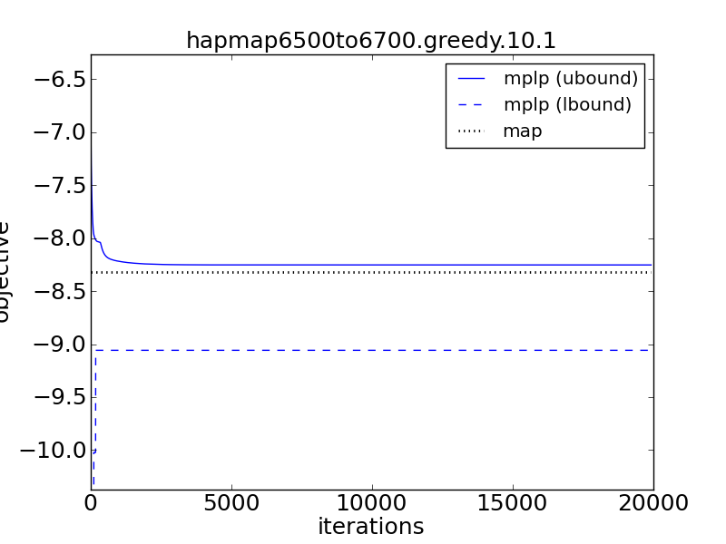
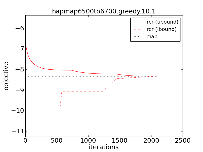
Figure 1: Recovering triplet clusters and equivalence constraints in MPLP (left) and RCR (right). Solid lines indicate the value of the dual objective (upper bound), dashed lines indicate the value of the current best assignment (lower bound), and the dotted line denotes the optimal MPE solution.

Figure 1 illustrates an example run of both MPLP and RCR, in a model where MPLP failed to find an optimal MPE solution. For the case of MPLP, one observes that MPLP starts to tighten the gap between its upper and lower bounds, but fails to tighten it further after some number of iterations. In fact, for this particular model, MPLP fails to find triplet clusters to introduce into its relaxation. On the other hand, RCR obtains the optimal solution after recovering only 70 of 451 equivalence constraints. When we look at the arithmetic circuits used to do inference in our simplified model, the size goes down from 38555 to 36729 nodes and edges after recovering 70 equivalence constraints.

In the following table, we summarized the number of recovered equivalence constraints needed to obtain an optimal solution, and the complexity of inference, for the two cases:

	# of models	avg. % recovered	avg. % increase in AC size
MPLP did not solve	13	26.93%	124.97%
RCR and MPLP solved	56	3.56%	99.65%

In the models that were left unsolved by MPLP, RCR was able to find exact MPE solutions by recovering only a quarter of the relaxed equivalence constraints, on average. This came with only a modest increase in the complexity of inference, i.e., AC size. In the models solved by both MPLP and RCR, very few equivalence constraints needed to be recovered on average, and in fact led to a very slight decrease in the complexity of inference.

We finally remark that the second set of experiments involved models that are not necessarily well suited for recovering triplet clusters with MPLP. Moreover, our comparisons with RCR were limited since we were restricted to models over binary variables (as recovery requires the use of a compensation algorithm like the one implied by Theorem 5, which is specific to binary variables). We plan more thorough empirical comparisons in future work.

7 Conclusion

In this paper, we formulated the technique of dual decomposition in the terms of Relax, Compensate and then Recover (RCR). By formulating dual decomposition in the more general terms of RCR, we have broadened the scope of the technique by (a) proposing new recovery heuristics for tightening the dual objective of dual decomposition, (b) extending it to other inference tasks, such as bounding the partition function (although this was not evaluated here), and (c) formulating it in terms that allows it to easily take advantage of the vast literature on exact inference, for the purposes of more effective approximate inference. Empirically, we showed how these new recovery heuristics can sometimes be used to obtain exact solutions to MPE problems, without increasing much the complexity of inference—in particular, on problems which existing systems based on dual decomposition are not as well suited for.

Acknowledgments

This work has been partially supported by NSF grant #IIS-1118122.

Appendix A Proofs

We first review and refine some notation and some definitions, for the purposes of our proofs. Here, variables are denoted by upper case letters ($X$) and their instantiations by lower case letters ($x$). Moreover, sets of variables are denoted by bold upper case letters (${\bf X}$) and their instantiations by bold lower case letters (${\bf x}$).

An MRF $\psi({\bf X})$, over a set of variables ${\bf X}$, is a product of factors $\psi_{i}$, which induces a probability distribution ${\it Pr}({\bf X})$:

$$\psi({\bf X})=\prod_{i}\psi_{i}({\bf X}_{i})\qquad\qquad\qquad{\it Pr}({\bf X})=\frac{1}{Z}\psi({\bf X}).$$

Here, each factor $\psi_{i}({\bf X}_{i})$ is a function mapping an instantiation ${\bf x}_{i}$ of variables ${\bf X}_{i}$, to a non-negative real number. Moreover, $Z=\sum_{{\bf x}}\psi({\bf x})$ is a normalizing constant called the partition function.

We are interested in approximations to the partition function, and the most probable explanation (MPE):

$$\mathsf{mpe}=\max_{{\bf x}}\psi({\bf x})$$

We refer to $\mathsf{mpe}$ as the MPE value, and a maximizing ${\bf x}$ as an MPE instantiation. We are also interested in MPE marginals $\mathsf{mpe}(x)$ and partition function marginals $Z(x)$:

$$\mathsf{mpe}(x)=\max_{{\bf x}\models x}\psi({\bf x})\qquad\qquad\qquad Z(x)=\sum_{{\bf x}\models x}\psi({\bf x})$$

where $\mathsf{mpe}(x)$ can be interpreted as the MPE value of our model, assuming variable $X$ takes on the value $x$; similarly for partition function marginals.

We may augment an MRF so that it contains factors ${eq}(X,Y)$ that represent equivalence constraints $X\equiv Y$ between pairs of variables $X$ and $Y$ in ${\bf X}$. For the purposes of this paper, we will assume that equivalence constraints arise by cloning a variable $X$ that appears in a factor $\psi_{i}({\bf X}_{i})$ (although our results hold for equivalence constraints in general). We will denote this clone by $X_{i}$, and assume an equivalence constraint ${eq}(X,X_{i})$. We continue to denote the set of original variables by ${\bf X}$, but we now denote the set of clone variables by ${\bf X}^{c}$. Our MRF with equivalence constraints is thus:

$$\psi({\bf X},{\bf X}^{c})=\prod_{i}\psi_{i}({\bf X}^{c}_{i})\cdot\prod_{X\equiv X_{i}}{eq}(X,X_{i})$$

Note that the distribution and the MPE problem (over the original variables ${\bf X}$), as well as the partition function, are all invariant to the introduction of equivalence constraints, as described above. Moreover, whenever we refer to a state $x$ of variable $X$, we will denote the corresponding state of the clone $X_{i}$ by $x_{i}$, unless otherwise stated.

We can relax an equivalence constraint ${eq}(X,X_{i})$ by removing its factor from the MRF, and then compensate for the relaxation by introducing two unit factors $\theta(X)$ and $\theta(X_{i})$. Doing so, for all equivalence constraints, we obtain a simpler MRF and distribution

$$\psi^{\prime}({\bf X},{\bf X}^{c})=\prod_{i}\psi_{i}({\bf X}^{c}_{i})\cdot\prod_{X\equiv X_{i}}\theta(X)\theta(X_{i})\qquad\qquad\qquad{\it Pr^{\prime}}({\bf X})=\frac{1}{Z^{\prime}}\psi^{\prime}({\bf X})$$

where $Z^{\prime}$ is the corresponding partition function. Note that each constraint ${eq}(X,X_{i})$ is associated with unique factors $\theta(X)$ and $\theta(X_{i})$, which we may sometimes distinguish by $\theta_{X_{i}}(X)$ and $\theta_{X}(X_{i})$.

Theorem 1

A compensation scheme for relaxed equivalence constraint ${eq}(X,X_{i})$ satisfies model-split iff the partition function $Z^{\prime}$ of the compensated model satisfies

$$\theta(x) =\alpha\frac{Z^{\prime}(x_{i})}{\theta(x_{i})} \theta(x_{i}) =\alpha\frac{Z^{\prime}(x)}{\theta(x)}$$ (1)

for all states $x,$ and their corresponding states $x_{i}$. Here, $\alpha$ is an arbitrary normalizing constant.

• See [3].   $\Box$

Theorem 2

A compensation scheme that satisfies upper-bound leads to a compensated model whose partition function is an upper bound on the exact partition function, and whose MPE value is an upper bound on the exact MPE value.

• Consider an equivalence constraint ${eq}(X,X_{i})$. If variable $X$ is set to the value $x$, and its clone $X_{i}$ is set to the corresponding value $x_{i}$, then ${eq}(x,x_{i})=1=\theta(x)\theta(x_{i})$ for a compensation satisfying upper-bound. When $x\neq x_{i}$, we have ${eq}(x,x_{i})=0\leq\theta(x)\theta(x_{i}).$ Moreover, $\psi({\bf x})=\psi^{\prime}({\bf x},{\bf x}^{c})$ if instantiation ${\bf x},{\bf x}^{c}$ satisfies all equivalence constraints, and $\psi({\bf x})=0\leq\psi^{\prime}({\bf x},{\bf x}^{c})$ when instantiation ${\bf x},{\bf x}^{c}$ does not. Thus, $0\leq\psi({\bf x})\leq\psi^{\prime}({\bf x},{\bf x}^{c})$ for all instantiations ${\bf x}$ and ${\bf x}^{c}$.

  The MPE of a compensated model is thus an upper bound on the MPE of the original:

  $$\max_{{\bf x}}\psi({\bf x})=\max_{{\bf x},{\bf x}^{c}:X\equiv X_{i}}\psi^{\prime}({\bf x},{\bf x}^{c})\leq\max_{{\bf x},{\bf x}^{c}}\psi^{\prime}({\bf x},{\bf x}^{c}).$$

  Here the second maximization is constrained to assignments ${\bf x},{\bf x}^{c}$ that satisfy all equivalence constraints ${eq}(X,X_{i})$. Similarly, for the partition function:

  $$Z=\sum_{{\bf x}}\psi({\bf x})=\sum_{{\bf x},{\bf x}^{c}:X\equiv X_{i}}\psi^{\prime}({\bf x},{\bf x}^{c})\leq\sum_{{\bf x},{\bf x}^{c}}\psi^{\prime}({\bf x},{\bf x}^{c})=Z^{\prime}.$$

  $\Box$

Theorem 3

For a single equivalence constraint ${eq}(X,X_{i})$, a compensation scheme satisfies pr-dd iff for all values $x,$ and their corresponding values $x_{i},$ the compensated model satisfies

$$\theta(x)=\left(\frac{Z^{\prime}(x_{i})/\theta(x_{i})}{Z^{\prime}(x)/\theta(x)}\right)^{\frac{1}{2}}\quad\quad\theta(x_{i})=\left(\frac{Z^{\prime}(x)/\theta(x)}{Z^{\prime}(x_{i})/\theta(x_{i})}\right)^{\frac{1}{2}}$$ (3)

The scheme satisfies mpe-dd iff it satisfies the above condition with $\mathsf{mpe}^{\prime}(.)$ substituted for $Z^{\prime}(.)$.

• From the definition of a pr-equivalence, we first have:

  $${\it Pr^{\prime}}(x)=\frac{1}{Z^{\prime}}\frac{\partial Z^{\prime}}{\partial\theta(x)}\theta(x)=\frac{1}{Z^{\prime}}\frac{\partial Z^{\prime}}{\partial\theta(x_{i})}\theta(x_{i})={\it Pr^{\prime}}(x_{i})$$

  for all values $x$, and $x_{i}$ respectively. For a compensation satisfying upper-bound, we can substitute $\theta(x_{i})=\frac{1}{\theta(x)}$ and solve for $\theta(x)$, giving us fixed-point conditions:

  $$\theta(x)=\left(\frac{\partial Z^{\prime}/\partial\theta(x_{i})}{\partial Z^{\prime}/\partial\theta(x)}\right)^{\frac{1}{2}}$$

  We further remark that $\frac{\partial Z^{\prime}}{\partial\theta(x)}$ is independent of the unit factor $\theta(x)$ since the partition function $Z^{\prime}$ is linear in $\theta(x)$. Moreover, we can compute $\frac{\partial Z^{\prime}}{\partial\theta(x)}$ by $\frac{Z^{\prime}(x)}{\theta(x)}$, when $\theta(x)$ is positive. Otherwise, partial derivatives can be computed efficiently in traditional frameworks for inference, as in [11, 12].

  The derivation is analogous for MPE, starting from the definition of mpe-equivalence.   $\Box$

Theorem 4

When the compensated model is fully decomposed, the fixed-point iterative updates of Equation 3 correspond precisely to the block coordinate descent updates of the sum-product and max-sum diffusion algorithms, respectively.

• Consider an MRF found by taking each factor $\psi_{i}({\bf X}_{i})$ and each variable $X\in{\bf X}_{i}$, and then:

  1. replace variable $X$ with a unique clone variable $X_{i}$, and

  2. introduce an equivalence constraint ${eq}(X,X_{i})$.

  When we relax all equivalence constraints, the resulting model is fully decomposed, where all of the factors $\psi_{i}({\bf X}^{c}_{i})$, now over clone variables ${\bf X}^{c}_{i}$, are disconnected. We add compensating factors $\theta_{X_{i}}(X)$ and $\theta_{X}(X_{i})$, where $X$ denotes the original variable and $X_{i}$ for each equivalence constraint ${eq}(X,X_{i})$ relaxed. The resulting MRF, over original variables ${\bf X}$ and clone variables ${\bf X}^{c}$ is:

  $$\psi^{\prime}({\bf X},{\bf X}^{c}) =\Big{[}\prod_{i}\psi_{i}({\bf X}^{c}_{i})\Big{]}\cdot\Big{[}\prod_{X\equiv X_{i}}\theta_{X_{i}}(X)\theta_{X}(X_{i})\Big{]}$$

  $$=\prod_{i}\Big{[}\psi_{i}({\bf X}^{c}_{i})\prod_{X_{i}\in{\bf X}^{c}_{i}}\theta_{X}(X_{i})\Big{]}\cdot\Big{[}\prod_{X}\prod_{i:X\in{\bf X}_{i}}\theta_{X_{i}}(X)\Big{]}.$$

  Note that each factor $\psi_{i}({\bf X}^{c}_{i})$ is now associated with a unit factor $\theta_{X}(X_{i})$ for each equivalence constraint ${eq}(X,X_{i})$ that the factor was involved in: one for each $X_{i}\in{\bf X}^{c}_{i}$. Each variable $X$ is associated with a unit factor $\theta_{X_{i}}(X)$ for each equivalence constraint ${eq}(X,X_{i})$ that variable $X$ was involved in: one for each factor $\psi_{i}({\bf X}_{i}),$ where $X\in{\bf X}_{i}$. Figure 2 highlights a decomposition for a simple MRF.

  

  

  Figure 2: On the left, is an MRF with two factors, $\psi_{1}(A,C,D)$ and $\psi_{2}(A,B,D)$. On the right, is the MRF found by cloning all variables, and then relaxing the 6 resulting equivalence constraints (indicated by dashed lines). Besides the two original factors, now over cloned variables, $\psi_{1}(A_{1},C_{1},D_{1})$ and $\psi_{2}(A_{2},B_{2},D_{2})$, we now have twelve compensating factors, two each for the six equivalence constraint relaxed: one factor $\theta(X)$ at each of the six cloned variables $X$, and one factor $\theta(X_{i})$ each for variables $B$ and $C$ (involved in one equivalence constraint), and two factors $\theta(X_{i})$ each for variables $A$ and $D$ (involved in two equivalence constraints).

Now, consider an equivalence constraint ${eq}(X,X_{i})$ in our compensated MRF $\mathcal{M}^{\prime}$. Since the MRF is disconnected, the factor $\theta_{X_{i}}(X)$ interacts only with the compensating factors over variable $X$. Similarly, the factor $\theta_{X}(X_{i})$ interacts only with the factor $\psi_{i}({\bf X}^{c}_{i})$, and the other compensating factors over the other clone variables in ${\bf X}^{c}_{i}$. Thus, our partial derivatives have the following form:

$$\frac{\partial Z^{\prime}}{\partial\theta_{X_{i}}(x)} \propto\prod_{\begin{subarray}{c}j:X\in{\bf X}_{j}\\ j\neq i\end{subarray}}\theta_{X_{j}}(x)$$

$$\frac{\partial Z^{\prime}}{\partial\theta_{X}(x_{i})} \propto\sum_{{\bf x}^{c}_{i}\models x_{i}}\psi({\bf x}^{c}_{i})\cdot\prod_{\begin{subarray}{c}Y_{i}\in{\bf X}^{c}_{i}:\\ Y\neq X\end{subarray}}\theta_{Y}(y_{i})$$

Note again that we can compute the partial derivatives $\frac{\partial Z^{\prime}}{\partial\theta_{X_{i}}(x)}$ by $\frac{Z^{\prime}(x)}{\theta_{X_{i}}(x)}$, when $\theta_{X_{i}}(x)$ is positive.

For the MPE problem, we are interested in computing $\frac{\mathsf{mpe}^{\prime}(x)}{\theta_{X_{i}}(x)}$, which has a form analogous to the above, except with maximizations instead of summations. Moreover, $\frac{\mathsf{mpe}^{\prime}(x)}{\theta_{X_{i}}(x)}$ is independent of the parameter $\theta_{X_{i}}(x)$ (after taking into account the division). The resulting fixed-point updates for the log parameters, are now:

$$\log\theta_{X_{i}}(x) =-\frac{1}{2}\frac{\mathsf{mpe}^{\prime}(x)}{\theta_{X_{i}}(x)}+\frac{1}{2}\frac{\mathsf{mpe}^{\prime}(x_{i})}{\theta_{X}(x_{i})}$$

$$=-\frac{1}{2}\sum_{\begin{subarray}{c}j:X\in{\bf X}_{j}\\ j\neq i\end{subarray}}\log\theta_{X_{j}}(x)+\frac{1}{2}\max_{{\bf x}^{c}_{i}\models x_{i}}\left[\log\psi_{i}({\bf x}^{c}_{i})+\sum_{\begin{subarray}{c}Y_{i}\in{\bf X}^{c}_{i}:\\ Y\neq X\end{subarray}}\log\theta_{Y}(y_{i})\right]+\log\alpha$$

$$=-\frac{1}{2}\sum_{\begin{subarray}{c}j:X\in{\bf X}_{j}\\ j\neq i\end{subarray}}\log\theta_{X_{j}}(x)+\frac{1}{2}\max_{{\bf x}^{c}_{i}\models x_{i}}\left[\log\psi_{i}({\bf x}^{c}_{i})-\sum_{\begin{subarray}{c}Y_{i}\in{\bf X}^{c}_{i}:\\ Y\neq X\end{subarray}}\log\theta_{Y_{i}}(y)\right]+\log\alpha$$

where we substitute $\log\theta_{Y}(y_{i})$ with $-\log\theta_{Y_{i}}(y)$, from our upper-bound condition. Here, $\alpha$ can be treated as a normalizing constant, which we can ignore, since it is canceled out in the joint distribution of the compensated MRF. We thus arrive at the block coordinate descent update of the max-sum diffusion algorithm, as in [8, Equation 1.17].   $\Box$

Theorem 5

For a single equivalence constraint ${eq}(X,X_{i})$, with binary variables $X$ and $X_{i}$, a compensation scheme satisfies pr-dd iff the compensated model satisfies

$$\frac{\theta(x)}{\theta(\bar{x})}=\left(\frac{Z^{\prime}(\bar{x},x_{i})/\theta(\bar{x})\theta(x_{i})}{Z^{\prime}(x,\bar{x}_{i})/\theta(x)\theta(\bar{x}_{i})}\right)^{\frac{1}{2}}\qquad\qquad\frac{\theta(x_{i})}{\theta(\bar{x}_{i})}=\left(\frac{Z^{\prime}(x,\bar{x}_{i})/\theta(x)\theta(\bar{x}_{i})}{Z^{\prime}(\bar{x},x_{i})/\theta(\bar{x})\theta(x_{i})}\right)^{\frac{1}{2}}$$ (4)

The scheme satisfies mpe-dd iff it satisfies the above condition with $\mathsf{mpe}^{\prime}(.)$ substituted for $Z^{\prime}(.)$.

• First, note that:

  $$\frac{Z^{\prime}(x,x_{i})}{\theta(x)\theta(x_{i})}=\frac{\partial^{2}Z^{\prime}}{\partial\theta(x)\partial\theta(x_{i})}$$ (5)

  which is a quantity that is independent of both of the unit factors $\theta(x)$ and $\theta(x_{i})$, since the partition function $Z^{\prime}$ is linear in $\theta(x)$, and linear in $\theta(x_{i})$.

  For binary variables $X$ and $X_{i}$ we have

  $${\it Pr}^{\prime}(x) = {\it Pr}^{\prime}(x,x_{i})+{\it Pr}^{\prime}(x,\bar{x}_{i})=\frac{1}{Z^{\prime}}\frac{\partial^{2}Z^{\prime}}{\partial\theta(x)\partial\theta(x_{i})}\theta(x)\theta(x_{i})+\frac{1}{Z^{\prime}}\frac{\partial^{2}Z^{\prime}}{\partial\theta(x)\partial\theta(\bar{x}_{i})}\theta(x)\theta(\bar{x}_{i})$$

  $${\it Pr}^{\prime}(x_{i}) = {\it Pr}^{\prime}(x,x_{i})+{\it Pr}^{\prime}(\bar{x},x_{i})=\frac{1}{Z^{\prime}}\frac{\partial^{2}Z^{\prime}}{\partial\theta(x)\partial\theta(x_{i})}\theta(x)\theta(x_{i})+\frac{1}{Z^{\prime}}\frac{\partial^{2}Z^{\prime}}{\partial\theta(\bar{x})\partial\theta(x_{i})}\theta(\bar{x})\theta(x_{i})$$

  After substituting $\theta(x_{i})=\frac{1}{\theta(x)}$ (from our upper-bounds condition), equating the above marginals, we get the desired result after some rearranging.   $\Box$

References

- [1] Arthur Choi and Adnan Darwiche. Relax, compensate and then recover. In Takashi Onada, Daisuke Bekki, and Eric McCready, editors, New Frontiers in Artificial Intelligence, volume 6797 of Lecture Notes in Computer Science, pages 167–180. Springer Berlin / Heidelberg, 2011.
- [2] Judea Pearl. Probabilistic Reasoning in Intelligent Systems: Networks of Plausible Inference. Morgan Kaufmann Publishers, Inc., San Mateo, California, 1988.
- [3] Arthur Choi and Adnan Darwiche. An edge deletion semantics for belief propagation and its practical impact on approximation quality. In Proceedings of the 21st AAAI Conference on Artificial Intelligence (AAAI), pages 1107–1114, 2006.
- [4] Arthur Choi and Adnan Darwiche. Approximating the partition function by deleting and then correcting for model edges. In Proceedings of the 24th Conference on Uncertainty in Artificial Intelligence (UAI), pages 79–87, 2008.
- [5] Gal Elidan and Amir Globerson. Summary of the 2010 UAI approximate inference challenge. http://www.cs.huji.ac.il/project/UAI10/summary.php, 2010.
- [6] Jason K. Johnson, Dmitry M. Malioutov, and Alan S. Willsky. Lagrangian relaxation for MAP estimation in graphical models. In Proceedings of the 45th Allerton Conference on Communication, Control and Computing, pages 672–681, 2007.
- [7] Nikos Komodakis, Nikos Paragios, and Georgios Tziritas. MRF optimization via dual decomposition: Message-passing revisited. In ICCV, pages 1–8, 2007.
- [8] David Sontag, Amir Globerson, and Tommi Jaakkola. Introduction to dual decomposition for inference. In Suvrit Sra, Sebastian Nowozin, and Stephen J. Wright, editors, Optimization for Machine Learning. MIT Press, 2011.
- [9] Arthur Choi and Adnan Darwiche. Relax then compensate: On max-product belief propagation and more. In Proceedings of the Twenty-Third Annual Conference on Neural Information Processing Systems (NIPS), pages 351–359, 2009.
- [10] Jonathan Yedidia, William Freeman, and Yair Weiss. Constructing free-energy approximations and generalized belief propagation algorithms. IEEE Transactions on Information Theory, 51(7):2282–2312, 2005.
- [11] Adnan Darwiche. A differential approach to inference in bayesian networks. Journal of the ACM, 50(3):280–305, 2003.
- [12] James Park and Adnan Darwiche. A differential semantics for jointree algorithms. Artificial Intelligence, 156:197–216, 2004.
- [13] Srinivas M. Aji and Robert J. McEliece. The generalized distributive law and free energy minimization. In Proceedings of the 39th Allerton Conference on Communication, Control and Computing, pages 672–681, 2001.
- [14] Rina Dechter, Kalev Kask, and Robert Mateescu. Iterative join-graph propagation. In Proceedings of the Conference on Uncertainty in Artificial Intelligence, pages 128–136, 2002.
- [15] Thomas P. Minka. A family of algorithms for approximate Bayesian inference. PhD thesis, MIT, 2001.
- [16] Martin J. Wainwright, Tommi Jaakkola, and Alan S. Willsky. Tree-based reparameterization framework for analysis of sum-product and related algorithms. IEEE Transactions on Information Theory, 49(5):1120–1146, 2003.
- [17] Jonathan S. Yedidia, William T. Freeman, and Yair Weiss. Understanding belief propagation and its generalizations. In Gerhard Lakemeyer and Bernhard Nebel, editors, Exploring Artificial Intelligence in the New Millennium, chapter 8, pages 239–269. Morgan Kaufmann, 2003.
- [18] Amir Globerson and Tommi Jaakkola. Fixing max-product: Convergent message passing algorithms for MAP LP-relaxations. In NIPS, pages 553–560, 2008.
- [19] David Sontag, Talya Meltzer, Amir Globerson, Tommi Jaakkola, and Yair Weiss. Tightening LP relaxations for MAP using message passing. In UAI, pages 503–510, 2008.
- [20] Chen Yanover, Talya Meltzer, and Yair Weiss. Linear programming relaxations and belief propagation — an empirical study. Journal of Machine Learning Research, 7:1887–1907, 2006.
- [21] Mark Chavira and Adnan Darwiche. Encoding CNFs to empower component analysis. In Proceedings of the 9th International Conference on Theory and Applications of Satisfiability Testing (SAT), pages 61–74. Springer Berlin / Heidelberg, Lecture Notes in Computer Science, Volume 4121, 2006.
- [22] Mark Chavira and Adnan Darwiche. Compiling Bayesian networks using variable elimination. In Proceedings of the 20th International Joint Conference on Artificial Intelligence (IJCAI), pages 2443–2449, 2007.
- [23] Arthur Choi, Trevor Standley, and Adnan Darwiche. Approximating weighted max-sat problems by compensating for relaxations. In Proceedings of the 15th International Conference on Principles and Practice of Constraint Programming (CP), pages 211–225, 2009.
- [24] Gal Elidan and Stephen Gould. Learning bounded treewidth Bayesian networks. JMLR, 9:2699–2731, 12 2008.