Sparse regression with highly correlated predictors

Abstract.

We consider a linear regression $y=X\beta+u$ where $X\in\mathbb{\mathbb{{R}}}^{n\times p},\;p\gg n,$ and $\beta$ is $s-$sparse. Motivated by examples in financial and economic data, we consider the situation where $X$ has highly correlated and clustered columns. To perform sparse recovery in this setting, we introduce the clustering removal algorithm (CRA), that seeks to decrease the correlation in $X$ by removing the cluster structure without changing the parameter vector $\beta$. We show that as long as certain assumptions hold about $X$, the decorrelated matrix will satisfy the restricted isometry property (RIP) with high probability. We also provide examples of the empirical performance of CRA and compare it with other sparse recovery techniques.

1. Introduction

We consider the sparse estimation (or sparse recovery) problem given by:

(1) $$\mbox{ Estimate $\beta$\ from }y=X\beta+u$$

where ${X}$ is a known $n\times p$ design matrix, $u$ is additive noise such that $\|u\|_{2}\leq\eta$ for some known $\eta$, and $\beta$ has at most $s$ non-zero entries with $s\ll n\ll p$. Lasso [13] and basis pursuit denoise (BPDN) [8] are popular sparse recovery approaches proposed for (1), which are based on solving certain convex optimization problems. On the other hand, orthogonal matching pursuit (OMP) [14], CoSaMP [12], Iterative Hard Thresholding [3], and Hard Thresholding Pursuit [10] are examples of greedy algorithms that can be used to solve (1). Although these algorithms have different capabilities in estimating $\beta$, the success of each is highly dependent on the structure of the design matrix $X$ and the sparsity level $s$ in relation to $p$ and $n$. It is well known that when the columns of $X$ have high empirical correlation, i.e., for some $i\neq j$, $\rho_{ij}:=\dfrac{X_{i}X_{j}^{*}}{||X_{i}||_{2}||X_{j}||_{2}}$ has magnitude close to one, the above mentioned sparse recovery methods do not perform well [4].

In many applications, such as in model selection, $X$ is already given in terms of observations of different variables of the data. Often, the variables constituting the columns of $X$ are highly correlated. Therefore, at least for a significant number of columns $i,j$, $|\rho_{ij}|$ tends to be close to 1, and accordingly, standard sparse recovery methods, such as the ones we mention above, fail to yield good estimates for $\beta$.

In this note, we will focus on this issue, i.e., sparse estimation when the design matrix has correlated columns. Motivated by various applications where $X$ is empirically generated, we will further assume that the columns of $X$ can be organized in a number of clusters such that the columns that are in the same cluster are highly correlated but the columns that are in different clusters may or may not be correlated. For example, let $X_{t,i}$ be the price of stock $i$ at time $t$. Due to shared underlying economic factors, we expect the price vector of, for example, technology stocks to be tightly clustered together. On the other hand, stocks of telecommunication companies may form a different cluster. Due to global economic factors, such as the monetary policy or the overall economic growth, the stock prices of telecommunication companies and technology companies may also be correlated, but we expect lower levels of correlation between them compared to the correlation inside the clusters. Another example where such cluster structure can be observed is in face recognition – see [19] for details.

Our approach can be summarized as follows: To overcome the challenge posed by high correlation in the design matrix, we propose to modify $X$ in order to get a matrix that is suitable for sparse recovery without changing the original parameter vector $\beta$. We seek to do this by first identifying the clusters (say, $q$ of them) and then constructing a representative vector for each cluster. Let $R\in\mathbb{R}^{n\times q}$ be the matrix constructed by putting together the representative vectors of the $q$ clusters. We project $X$ to the orthogonal complement of the range of $R$ and normalize the columns of the resulting matrix, which we denote by $\tilde{X}$. Our proposed algorithm, we will prove, is effective when this matrix $\tilde{X}$ is suitable as a compressive sensing measurement matrix.

After introducing our notation and the necessary background in Section 2, we state the proposed clustering removal algorithm (CRA) and our main assumptions in Section 3. In Section 4, we prove that if $X$ is a realization of a random matrix $\mathbf{X}$ whose columns are uniformly distributed on $q$ disjoint spherical caps, $\tilde{{X}}$ provides a suitable matrix for sparse recovery with high probability. In Section 5 we demonstrate the performance of our algorithm on highly correlated financial data, in comparison with BPDN and with SWAP, an algorithm proposed by [17] for sparse recovery in highly correlated settings.

2. Notations and Background

In what follows, we refer to random matrices and random vectors with bold letters. Let $n,r\in\mathbb{N}$ and let $A\in\mathbb{R}^{n\times r}$. We denote the $i$th column of $A$ by $A_{i}$. For $T\subseteq[r]:=\{1,\dots,r\}$, $A_{T}$ denotes the submatrix of $A$ consisting of its columns indexed by $T$. We define $\Pi_{A}$ to be the orthogonal projection operator into $\mathcal{R}(A)$, the range of $A$, and $\Pi_{A^{\perp}}$ denotes the orthogonal projection operator into the orthogonal complement of $\mathcal{R}(A)$. The best $k$-term approximation of $b\in\mathbb{R}^{n}$ is $b^{\{k\}}\in\mathbb{R}^{n}$ such that $b_{i}^{\{k\}}=b_{i}$ if $b_{i}$ is among the $k$ largest-in-magnitude entries of $b$. Otherwise, $b_{i}^{\{k\}}=0$. The corresponding best $k$-term approximation error in $\ell_{p}$ is

$$\sigma_{k}(b)_{\ell_{p}}:=\|b-b^{\{k\}}\|_{p}.$$

For $\Omega\subset S^{n-1}:=\{x\in\mathbb{R}^{n}:\|x\|_{2}=1\}$, we define the wedge $W(\Omega)$ by

$$W(\Omega):=\{rx:x\in\Omega,r\in[0,1]\}.$$

We denote the $n$-dimensional Lebesgue measure with $\lambda^{n}$, and the uniform spherical measure on $S^{n-1}$ with $\sigma^{n-1}$, which can be defined via

$$\sigma^{n-1}(\Omega):=\lambda^{n}(W(\Omega))/\lambda^{n}(W(S^{n-1}))$$

provided that $W(\Omega)$ is a measurable subset of $\mathbb{R}^{n}$ (otherwise $\Omega$ is not measurable). It should be noted that although different definitions of uniform spherical measure exist in the literature, all these measures must be equal, for example, in the setting that we have described above [7].

2.1. Compressive sampling

It is well known in the compressive sampling literature that BPDN provides a stable and robust solution for the sparse estimation problem (1) in a computationally tractable way , e.g., [8, 6]. Specifically, BPDN provides the estimate

(2) $$\beta_{\rm{BPDN}(y,\;X,\;\eta)}^{\#}:=\arg\min_{z}||z||_{1}\;s.t\quad||Xz-y||_{2}\leq\eta$$

where $\eta$ is an upper bound on $||u||_{2}$. One can guarantee that $\beta_{\rm{BPDN}(y,\;X,\;\eta)}^{\#}$ is a good estimate of $\beta$ if $\beta$ is sufficiently sparse or compressible (i.e., it can be well approximated by a sparse vector) and the “restricted isometry constants” of $X$ are sufficiently small [6], where the restricted isometry constants are defined as follows.

Definition 1.

Let $\delta_{s}(X)$ be the smallest positive constant such that $\forall T\subset[p],$ $|T|=s$, $\forall z\in\mathbb{R}^{s}$

$$(1-\delta_{s}(X))||z||_{2}^{2}\leq||X_{T}z||_{2}^{2}\leq(1+\delta_{s}(X))||z||_{2}^{2}.$$

In this case, we say that $X$ satisfies the restricted isometry property (RIP) of order $s$ with (restricted isometry) constant $\delta_{s}$.

The following theorem by [5] is a sharper version of the original “stable and robust recovery theorem” of [6].

Theorem 2.

Let $\delta_{ts}(X)<\sqrt{\frac{t-1}{t}}$ for some $t\geq\dfrac{4}{3}$. Then, for any $s$-sparse $\beta\in\mathbb{R}^{p}$,

$$||\beta_{\rm{BPDN}(y,\;X,\;\eta)}^{\#}-\beta||_{2}\leq\dfrac{C\sigma_{s}(\beta)_{\ell_{1}}}{\sqrt{s}}+D\eta$$

where $\beta_{\rm{BPDN}(y,\;X,\;\eta)}$ is as in (2), and $C,D>0$ are constants depending only on $\delta_{ts}$.

Even though the above theorem provides guarantees for BPDN to recover (or estimate) a sparse or compressible vector $\beta$ from its (possibly noisy) compressive samples $y$, these guarantees depend on $X$ having small restricted isometry constants. Constructing matrices with (nearly) optimally small restricted isometry constants is an extremely challenging task and still an open problem. Furthermore, computing these constants entails a combinatorial computational complexity and is not tractable as the size of the matrix increases. As a remedy, the literature has focused on random matrices. Indeed, one can prove that certain classes of sub-Gaussian random matrices (see next section) have nearly optimally small restricted isometry constants with overwhelming probability. Accordingly, realizations of such random matrices are used in the context of compressed sensing. We will adopt such an approach.

2.2. Sub-Gaussian random matrices

Our theoretical analysis in Section 4 relies on certain fundamental properties of sub-Gaussian random matrices. Here, we state some basic definitions that we will need. See [18] for a thorough exposition on the non-asymptotic theory of sub-Gaussian random matrices. In what follows, we stick to the notation of [18].

Definition 3.

A random variable $\mathbf{x}$ is said to be a sub-Gaussian random variable if it satisfies

$$\big{(}\mathbb{E}|\mathbf{x}|^{q}\big{)}^{1/q}\leq K\sqrt{q}$$

for all $q\geq 1$. Its sub-Gaussian norm $\|\mathbf{x}\|_{\psi_{2}}$ is defined as

$$\|\mathbf{x}\|_{\psi_{2}}=\sup_{q\geq 1}q^{-1/2}\big{(}\mathbb{E}|\mathbf{x}|^{q}\big{)}^{1/q}.$$

Next we define the following two important classes of random vectors.

Definition 4.

Let $\mathbf{x}$ be a random vector in $\mathbb{R}^{n}$.

1. $\mathbf{x}$ is said to be isotropic if $\mathbb{E}\langle\mathbf{x},u\rangle^{2}=\|u\|^{2}$ for all $u\in\mathbb{R}^{n}$.

2. $\mathbf{x}$ is sub-Gaussian if the marginals $\langle\mathbf{x},u\rangle$ are sub-Gaussian random variables for all $u\in\mathbb{R}^{n}$. The sub-Gaussian norm of the random vector $\mathbf{x}$ is defined by

   $$\|\mathbf{x}\|_{\psi_{2}}:=\sup_{u\in S^{n-1}}\|\langle\mathbf{x},u\rangle\|_{\psi_{2}}.$$

3. Assumptions and the Algorithm

We now go back to the sparse estimation problem (1), i.e., we want to estimate $\beta$ from $y=X\beta+u$ when given the matrix $X$ and the fact that $\|u\|_{2}\eta$. For the purpose of this paper, we assume that $||X_{i}||_{2}=1$ $\forall i\in[p]$. This simply can be done by normalizing the columns and rescaling $\beta$. Below, $C_{z}$ denotes a spherical cap, i.e., a portion of $S^{n-1}$ cut off by some hyperplane $P$, with “centroid” $z$, which is the point on the cap that has maximum distance from $P$.

We make the following additional assumptions.

Assumption 1.

The data matrix $X$ is a realization of a random matrix $\mathbf{X}$.

Assumption 2.

There exist $z_{1},\dots,z_{q}\in S^{n-1}$, $q\ll n$, such that $\forall i\in[p],\;\exists j\in[q]$ s.t $\mathbf{X_{i}}$ is uniformly distributed on $C_{z_{j}}$. That is, $\mathbf{X_{i}}$ is distributed according to the measure $m_{C_{z_{j}}}$, where for all measurable subsets $A$ of $C_{z_{j}}$,

$$m_{C_{z_{j}}}(A):=\lambda^{n}(W(A))/\lambda^{n}(W(C_{z_{j}})).$$

In this case, we write $\mathbf{X}_{i}\sim C_{z_{j}}$.

Assumption 3.

For $i\neq j$, $\mathbf{X_{i}}$ and $\mathbf{X_{j}}$ are independent.

Clearly, by Assumption 2, $X_{i}$ can be clustered into $q$ groups $G_{1},\dots,G_{q}$ where

$$G_{j}=\{i\in[p]\;s.t.\;\mathbf{X}_{i}\sim C_{z_{j}}\}$$

Algorithm 1 Clustering Removal Algorithm (CRA)

Step 1::

Estimate $G_{1},G_{2},...,G_{q}$.

Step 2::

Estimate $R:=[z_{1}|z_{2}|...|z_{q}]$ by setting $\hat{{z_{i}}}={\displaystyle\frac{1}{|G_{i}|}\sum_{j\in G_{i}}X_{j}}$.

Step 3::

Use a sparse recovery method for obtaining an estimate $\hat{\gamma}$ for $\gamma$ from

(3) $$\tilde{y}=\tilde{X}\gamma+\tilde{u}$$

where $\tilde{y}=\Pi_{R^{\perp}}y$, $\tilde{X}=\Pi_{R^{\perp}}XN_{\Pi_{R^{\perp}}X}^{-1}$, $\tilde{u}=\Pi_{R^{\perp}}u$.

Step 4::

The estimated $\beta$ will be $\hat{{\beta}}:=N_{\Pi_{R^{\perp}}X}^{-1}\hat{\gamma}$

Under these assumptions, we propose the clustering removal algorithm (CRA), described in Algorithm 1, for estimating $\beta$ in (1). In the first step of CRA, we estimate $G_{j}$, $j\in[q]$ by clustering the columns of $X$ using an appropriate clustering algorithm. For the numerical simulations in this paper, we use $k$-means clustering. Note that here we make the additional assumptions that we know $q$ and it is possible to estimate $G_{j}$, which, for example, requires that the spherical caps $C_{z_{j}}$ are well separated. In step 2, we estimate the centroid $z_{j}$ of each cluster $G_{j}$ by averaging the columns of $X$ that belong to $G_{j}$. Note that this is an unbiased estimate for $z_{j}$ assuming the clusters have been accurately identified. In step 3, we project each column of $X$ onto the orthogonal complement of the $q$-dimensional subspace spanned by the cluster centroids (without loss of generality, we assume that the set of cluster centroids $\{z_{1},\dots,z_{q}\}$ is linearly independent). We normalize the projected columns by multiplying the matrix with a diagonal matrix $N_{\Pi_{R^{\perp}}X}^{-1}$ where $(N_{\Pi_{R^{\perp}}X})_{i,i}=||\Pi_{R^{\perp}}X_{i}||_{2}$. After normalization, we obtain our modified matrix $\widetilde{X}:=\Pi_{R^{\perp}}XN_{\Pi_{R^{\perp}}X}^{-1}$ which, as we will show in the next section, is an appropriate measurement matrix for sparse recovery. The main idea here is that the columns of $\widetilde{X}$ lie on the $(n-q)$-dimensional subspace $\mathcal{R}(R)^{\perp}$ and, in fact, we show below that $\widetilde{X}$ is a realization of $\widetilde{\mathbf{X}}:=\Pi_{R^{\perp}}\mathbf{X}N_{\Pi_{R^{\perp}}\mathbf{X}}^{-1}$ where $\widetilde{\mathbf{X}_{i}}$ are independent and uniformly distributed on $S^{n-1}\cap\mathcal{R}(R)^{\perp}$. Accordingly, $\widetilde{X}$ turns out to be a good compressive sampling matrix, as explained in the next section, and we use a sparse recovery algorithm of our choice to obtain $\hat{\gamma}$, an estimate of $\gamma$, from (3). In the final step, we “unnormalize” by multiplying $\hat{\gamma}$ with the diagonal matrix $N_{\Pi_{R^{\perp}}X}^{-1}$.

4. Theoretical Recovery Guarantees for CRA

In this section, we assume that the clusters $G_{j}$ and their centroids $z_{j}$, $j=1,\dots,q$ are known (or accurately estimated). Under this assumption, we show that $\widetilde{\mathbf{X}}$, with high probability, is an appropriate compressive sampling matrix. The following two theorems from [18] will be instrumental in our theoretical analysis of CRA.

Theorem 5.

[18, Theorem 5.65] Let $\mathbf{Z}$ be an $n\times p$ random matrix with $n<p$ and $||\mathbf{Z_{i}}||_{2}=1$ for all $i\in[p]$. Let $k\in[p]$ and $\delta\in(0,1).$ Suppose that

1. the columns of $\mathbf{Z}$ are independent, and

2. the columns of $\sqrt{n}\mathbf{Z}$ are sub-Gaussian and isotropic.

Then, there exists positive constants $c$ and $C$, depending only on the maximum sub-Gaussian norm $K:=\max_{i}\|\mathbf{X}_{i}\|_{\psi_{2}}$ of the columns of $\mathbf{Z}$, such that

(4) $$n\geq C\delta^{-2}k\log(\frac{ep}{k})\implies\delta_{k}(\mathbf{Z})\leq\delta$$

with probability at least $1-2\exp(-c\delta^{2}n)$.

Theorem 6.

[18] Let $\mathbf{z}$ be an $n\times 1$ random vector. If $\mathbf{z}$ is uniformly distributed on $\sqrt{n}S^{n-1},$ then $\mathbf{z}$ is both sub-Gaussian and isotropic. Furthermore, the sub-Gaussian norm of $\mathbf{z}$ is bounded by a universal constant.

Next, we will prove that the columns of $\widetilde{\mathbf{X}_{i}}$ satisfy the hypotheses of Theorem 5. To that end, for $z\in\mathbb{R}^{n}$ define

$$\omega(z):=\begin{cases}0_{n\times 1}&\text{if $\Pi_{R^{\perp}}z=0$,}\\ \frac{\Pi_{R^{\perp}}z}{\left\|\Pi_{R^{\perp}}z\right\|_{2}}&\text{otherwise.}\end{cases}$$

Note that $\widetilde{\mathbf{X}_{i}}=\omega(\mathbf{X}_{i})$.

Theorem 7.

If Assumption 2 and Assumption 3 hold, $\omega(\mathbf{X}_{i})$ is uniformly distributed on $S^{n-1}\cap\mathcal{R}(R)^{\perp}$ for each $i\in[n]$. Moreover, for $i\neq j,$ $\omega(\mathbf{X}_{i})$ and $\omega(\mathbf{X}_{j})$ are independent.

Proof.

Since $\mathbf{X}_{i}$ and $\mathbf{X}_{j}$ are independent, and $\omega:\mathbb{R}^{n}\mapsto\mathbb{R}^{n}$ is measurable, $\omega(\mathbf{X}_{i})$ and $\omega(\mathbf{X}_{j})$ are also independent. Next we show that $\omega(\mathbf{X}_{i})$ is uniformly distributed on $S^{n-1}\cap\mathcal{R}(R)^{\perp}$. To that end, let $\mathbf{X}_{i}\in C_{R_{1}}$ and let $P$ be the hyperplane that generates $C_{R_{1}}.$ Then, $R_{1}$ is a normal vector of $P$ and accordingly we have

$$P=\{x\in\mathbb{R}^{n}:\langle x-q,R_{1}\rangle=0\}$$

where $q$ is an arbitrary point on $P$ that we fix. Recall, on the other hand, that

(5) $$C_{R_{1}}=\{x\in S^{n-1}:\langle x,R_{1}\rangle\geq\langle q,R_{1}\rangle\}$$

where $q\in P$ is as above. Note that $\langle q,R_{1}\rangle$ is independent of the choice of $q$.

Now, let $\Omega\subset S^{n-1}\cap\mathcal{R}(R)^{\perp}$. Noting that $||\mathbf{X_{i}}||_{2}=1$, we observe that

(6) $$\mathbb{P}(\omega(\mathbf{X_{i}})\in\Omega) =\mathbb{P}(\Pi_{R^{\perp}}\mathbf{X_{i}}\in W(\Omega)\setminus\{\mathbf{0}\})$$

(7) $$=\mathbb{P}(\Pi_{R^{\perp}}\mathbf{X_{i}}\in W(\Omega))-\mathbb{P}(\Pi_{R^{\perp}}\mathbf{X_{i}}=\mathbf{0})$$

since $\mathbf{0}\in W(\Omega)$. We know that any vector $z\in\mathbb{R}^{n}$ can be uniquely written as $z_{R}+z_{R^{\perp}}$ where $z_{R}\in\mathcal{R}(R)$ and $z_{R^{\perp}}\in\mathcal{R}(R)^{\perp}$. Note that $\Pi_{R^{\perp}}z=\Pi_{R^{\perp}}z_{R}+\Pi_{R^{\perp}}z_{R^{\perp}}=z_{R^{\perp}}$. Therefore, $\Pi_{R^{\perp}}z\in W(\Omega)$ if and only if $z_{R^{\perp}}\in W(\Omega)$ which is holds if and only if $z$ is an element of

$$\Pi^{-1}(\Omega):=\{ru+Rv:\ r\in[0,1],\;u\in\Omega,\;v\in\mathbb{R}^{q}\}.$$

Hence, keeping in mind that $\mathbf{X}_{i}\in C_{R_{1}}$, we have

$$\mathbb{P}(\Pi_{R^{\perp}}\mathbf{X_{i}}\in W(\Omega))=\mathbb{P}(\mathbf{X_{i}}\in\Pi^{-1}(\Omega)\cap C_{R_{1}})$$

and

$$\mathbb{P}(\Pi_{R^{\perp}}\mathbf{X_{i}}=\mathbf{0})=\mathbb{P}(\mathbf{X_{i}\in}\mathcal{R}(R)\cap C_{R_{1}}).$$

Furthermore, since the distribution of $\mathbf{X_{i}}$ is continuous, and $\mathcal{R}(R)$ has a lower dimension compared to $C_{R_{1}}$, $\mathbb{P}(\mathbf{X_{i}\in}C_{R_{1}}\cap\mathcal{R}(R))=0$. Accordingly, it follows from (7) that

(8) $$\mathbb{P}(\omega(\mathbf{X_{i}})\in\Omega)=\mathbb{P}(\mathbf{X_{i}}\in\Pi^{-1}(\Omega)\cap C_{R_{1}}).$$

Next, recall that $\mathbf{X}_{i}$ is uniformly distributed on $C_{R_{1}}$, i.e., $\mathbf{X}_{i}$ is distributed according to the measure $m_{C_{R_{1}}}$, defined as in Assumption 2. Therefore, we can rewrite (8) as

$$\mathbb{P}(\omega(\mathbf{X_{i}})\in\Omega) =\int\limits_{\Pi^{-1}(\Omega)\cap C_{R_{1}}}dm_{C_{R_{1}}}$$

$$=\int\limits_{W(\Pi^{-1}(\Omega)\cap C_{R_{1}})}\frac{d\lambda^{n}(y)}{\lambda^{n}(W(C_{R_{1}}))}$$

$$=\int\limits_{\Pi^{-1}(\Omega)\cap W(C_{R_{1}})}\frac{d\lambda^{n}(y)}{\lambda^{n}(W(C_{R_{1}}))}$$

(9) $$=\int\limits_{\Pi^{-1}(\Omega))}\mathbbm{1}_{W(C_{R_{1}})}(y)\dfrac{1}{\lambda^{n}(W(C_{R_{1}}))}d\lambda^{n}(y)$$

where $\mathbbm{1}_{W(C_{R_{1}})}$ is the indicator function of the set $W(C_{R_{1}})$, i.e.,

$$\mathbbm{1}_{W(C_{R_{1}})}(y):=\begin{cases}1&\mbox{if $y\in W(C_{R_{1}})$}\\ 0&\text{otherwise}\end{cases}.$$

Above, the second equality follows from the definition of the measure $m_{C_{R_{1}}}$ and the third equality holds because $W(\Pi^{-1}(\Omega)\cap C_{R_{1}})=\Pi^{-1}(\Omega)\cap W(C_{R_{1}})$, which is easy to verify.

Next, we decompose $\Pi^{-1}(\Omega)=W(\Omega)\times\mathcal{R}(R)$ and denote by $\lambda^{q}$ and $\lambda^{n-q}$ the Lebesgue measure on $\mathcal{R}(R)$ and on $\mathcal{R}(R)^{\perp}$ respectively. Note that $W(\Omega)$ and $\mathcal{R}(R)$, and thus every $y\in\Pi^{-1}(\Omega)$ can be uniquely decomposed as $y=y_{R^{\perp}}+y_{R}$ such that $y_{R^{\perp}}\in W(\Omega)$ and $y_{R}\in\mathcal{R}(R)$. Then, we obtain

$$\mathbb{P}(\omega(\mathbf{X_{i}})\in\Omega)\hskip-54.06006pt$$

$$=\int\limits_{W(\Omega)}\left[\int\limits_{\mathcal{R}(R)}\frac{\mathbbm{1}_{W(C_{R_{1}})}(y_{R^{\perp}}+y_{R})}{\lambda^{n}(W(C_{R_{1}}))}\;d\lambda^{q}(y_{R})\right]\;{{d\lambda^{n-q}}(y_{R^{\perp}})}$$

(10) $$={\scriptstyle\int\limits_{\Omega}\int\limits_{[0,1]}\left[\int\limits_{\mathcal{R}(R)}\frac{\mathbbm{1}_{W(C_{R_{1}})}(ru+y_{R})}{\lambda^{n}(W(C_{R_{1}}))}d\lambda^{q}(y_{R})\right]r^{{\scriptstyle n-q-1}}dr\;{\scriptstyle d\sigma^{n-q-1}(u)}}$$

Above, first equality follows from Fubini-Tonelli’s theorem, and the second equality is obtained by passing to polar coordinates and using Fubini-Tonelli’s theorem one more time. Finally, $\sigma^{n-q-1}$ is the unique spherical measure on $S^{n-1}\cap\mathcal{R}(R)^{\perp}$, i.e., the unit sphere of the subspace $\mathcal{R}(R)^{\perp}$.

Next, we observe that $\mathbbm{1}_{W(C_{R_{1}})}(ru+y_{R})=1$ if and only if one of the following two statements hold:

1. $ru+y_{R}=0$, which, since $u$ is orthogonal to $y_{R}$, is equivalent to having $r^{2}+\|y_{R}\|_{2}^{2}=0$, or

2. $0<r^{2}+\|y_{R}\|_{2}^{2}\leq 1$ and

   $$\frac{ru+v}{||ru+v||_{2}}\in C_{R_{1}}$$

   which, by (5), holds if and only if

   $$\langle y_{R},R_{1}\rangle\geq\big{(}r^{2}+\|y_{R}\|_{2}^{2}\big{)}^{1/2}\langle q,R_{1}\rangle$$

   where $q$ is as in (5).

Accordingly, we conclude that the innermost integral in (10) does not depend on $u$, which implies that

(11) $$\int\limits_{[0,1]}\left[\int\limits_{\mathcal{R}(R)}\frac{\mathbbm{1}_{W(C_{R_{1}})}(ru+y_{R})}{\lambda^{n}(W(C_{R_{1}}))}d\lambda^{q}(y_{R})\right]r^{{\scriptstyle n-q-1}}dr=c,$$

where $c$ is a constant that only depends on $n$. Substituting (11) into (10), we obtain

$$\mathbb{P}(\omega(\mathbf{X_{i}})\in\Omega)=c\sigma^{n-q-1}(\Omega).$$

Therefore, we conclude that $\omega(\mathbf{X_{i}})$ is uniformly distributed on $S^{n-1}\cap\mathcal{R}(R)^{\perp}$.∎

Next, we will show that $\mathbf{\tilde{X}}$, with high probability, is an appropriate compressive sampling matrix, and thus we can use the proposed clustering removal algorithm (CRA) to obtain an accurate estimate of $\beta$ in (1). To that end, let $U^{T}:\mathbb{R}^{n}\mapsto\mathbb{R}^{n}$ be a unitary transformation such that $U^{T}(\mathcal{R}(R)^{\perp})=\text{span}\{e_{1},\dots,e_{n-q}\}$ where $e_{i}$ are the standard basis vectors. Then we can write

$$U^{T}\widetilde{\mathbf{X}}=\begin{bmatrix}\textbf{A}\\ 0_{q\times p}\end{bmatrix}$$

where A is a $(n-q)\times p$ random matrix. Due to the rotation invariance of the Lebesgue measure, and since $U$ is a deterministic matrix, the columns of $U^{T}\widetilde{\textbf{X}}$ are independently uniformly distributed over

$$U^{T}(S^{n-1}\cap\mathcal{R}(R)^{\perp})=\{x\in S^{n-1}:\ x_{n-q+1}=...=x_{n}=0\}.$$

This means that the columns of $\mathbf{A}$ are uniformly distributed over $S^{n-q-1}$. Theorem 5 and Theorem 6 provide sufficient conditions for A to satisfy RIP with overwhelming probability. More precisely, the following holds.

Corollary 8.

If $(n-q)\geq C\delta^{-2}k\log(\frac{ep}{k})$, then with probability at least $1-2\exp(-c\delta^{2}(n-q))$, $\delta_{k}(\textbf{A})\leq\delta$.

Next, noting that $\widetilde{\mathbf{X}}=U\begin{bmatrix}\textbf{A}\\ 0_{q\times p}\end{bmatrix}$, we relate the RIP constants of $\mathbf{\widetilde{X}}$ with the RIP constants of $\mathbf{A}$.

Proposition 9.

If $A$ satisfies the restricted isometry property with constant $\delta_{k}$, $U\begin{bmatrix}A\\ 0_{q\times p}\end{bmatrix}$ will also satisfy RIP with the exact same constant.

Proof.

First, recall that a matrix $Z\in\mathbb{R}^{n\times p}$ satisfies RIP of order $k$ with constant $\delta_{k}$ if and only if for all $I\subset[p]$ with $|I|=k$, the eigenvalues of $Z^{T}_{I}Z_{I}$ are all between $1-\delta_{k}$ and $1+\delta_{k}$. Here $Z_{I}$ denotes the submatrix of $Z$ consisting of its columns indexed by $I$.

Suppose that $A$ satisfies RIP of order k with constant $\delta_{k}$. Set

$$\widetilde{X}=U\begin{bmatrix}A\\ 0_{q\times p}\end{bmatrix}$$

and let $I$ be any subset of $[p]$ such that $|I|=k$. Then,

$$\widetilde{X}^{T}_{I}\widetilde{X}_{I} =\Big{(}U\begin{bmatrix}A_{I}\\ 0_{q\times k}\end{bmatrix}\Big{)}^{T}\Big{(}U\begin{bmatrix}A_{I}\\ 0_{q\times k}\end{bmatrix}\Big{)}$$

$$={\begin{bmatrix}A_{I}\\ 0_{q\times k}\end{bmatrix}}^{T}U^{T}U\begin{bmatrix}A_{I}\\ 0_{q\times k}\end{bmatrix}$$

$$=A_{I}^{T}A_{I}.$$

Therefore, for all $I\subset[p]$, eigenvalues of $\widetilde{X}_{I}^{T}\widetilde{X}_{I}$ and $A_{I}^{T}A_{I}$ are equal. Hence, $\widetilde{X}$ satisfies RIP of order $k$ with constant $\delta_{k}$ if $A$ satisfies RIP of order $k$ with the same constant. ∎

Proposition 9 suggests that if the assumptions of Corollary 8 are met, $\widetilde{\textbf{X}}$ satisfies RIP with overwhelming probability. This, in turn, provides uniform estimation guarantees for $\gamma$, as defined in (3). In particular, combining Corollary 8 and Proposition 9, we arrive at the following conclusion.

Theorem 10.

Consider Problem 1 and suppose that the data matrix $X$ satisfies Assumptions 1-3.

1. If $(n-q)\geq C(t-1)s\log(\frac{ep}{ts})$ for some $t\geq 4/3$, then $\delta_{ts}(\widetilde{X})\leq\sqrt{\frac{t-1}{t}}$ with probability greater than $1-\exp\big{(}-c\frac{t-1}{t}(n-q)\big{)}$.

2. Consequently, for any $s$-sparse $\gamma\in\mathbb{R}^{p}$,

   $$||\gamma_{BPDN(\eta)}^{\#}-\gamma||_{2}\leq D\eta+\frac{2C\sigma_{s}(\gamma)_{\ell_{1}}}{\sqrt{s}}$$

   where $D,C$>0 are constants depending only on $\delta_{ts}$. Here $\gamma$ is as in (3).

3. The estimate in (ii) implies the following bound for the estimate of $\beta$:

   $$||\hat{{\beta}}-\beta||_{2}\leq\max_{i}\dfrac{1}{||\Pi_{R^{\perp}}X_{i}||_{2}}\big{(}D\eta+\dfrac{2C\sigma_{1}(\gamma)}{\sqrt{s}}\big{)}.$$

Remark 1.

Note that part (i) of Theorem 10 is a restatement of Corollary 8 with $\delta=\sqrt{\frac{t-1}{t}}$ and $k=ts$. In particular, we can set $t=2$, which yields the sufficient condition

$$(n-q)\geq Cs\log\big{(}\frac{ep}{2s}\big{)}.$$

Part (ii) of Theorem 10 follows from Theorem 9 together with part (i). Part (iii) can be justified using the definition of $\gamma$ as well as Step 4 of Algorithm 1.

Remark 2.

Part (iii) of Theorem 10 shows that in the estimation of $\beta$ the error term is inflated and behaves like $\max(1/||\Pi_{R^{\perp}}X_{i}||_{2})$. However, it should be noted that no matter what method is used, sparse recovery in highly correlated settings is inherently unstable when the noise level is high. For example, let $X_{i}$ and $X_{j}$ be unit-norm and highly correlated, and let $T_{\beta}$ be the indices of the true support of $\beta$. Assume $i\in T_{\beta}$ but $j\not\in T_{\beta}$. Then, without any assumptions on the structure of the noise $u$, as soon as $||u||_{2}$ exceeds $||X_{i}-X_{j}||_{2}|\beta_{i}|$ it becomes impossible to distinguish whether $i\in T_{\beta}$ or $j\in T_{\beta}$ by just considering $y$. If $X_{i}$ and $X_{j}$ are highly correlated, then $\left\|X_{i}-X_{j}\right\|_{2}$ tends to be small and unless $\beta_{i}$ is extremely large, $||X_{i}-X_{j}||_{2}|\beta_{i}|$ tends to be small too. Hence, nearly accurate sparse recovery is possible only for modest amounts of $||u||_{2}$. As we will see in section 5, the numerical results corroborate this result.

Remark 3.

Our analysis in this section has been based on the (unrealistic) assumption that $\mathcal{R}(R)^{\perp}$ can be perfectly estimated. Let $E$ be an imperfect estimate of $\mathcal{R}(R)^{\perp}$. By some algebra it can be shown that if $E$ is reasonably accurate, one can bound the matrix norm of the difference of $\widetilde{X}$ and $\widehat{X}:=\Pi_{E}XN_{\Pi_{E}X}^{-1}$. From there on we refer the reader to the analysis of [11] which suggests that $\widehat{X}$ will still satisfy the restricted isometry property but with different constants, which depend on the restricted isometry constants of $\widetilde{X}$ and the accuracy of $E$. We also note that the numerical experiments we present in the next section use design matrices for which clusters or $\mathcal{R}(R)^{\perp}$ are not known a priori and can only be imperfectly estimated. Yet, the empirical results illustrate that CRA is still effective in these examples.

5. Empirical Performance

For the purpose of testing the empirical performance of our algorithm, we provide two sets of experiments. In the first one, we generate $X$ synthetically from a factor model. In the second experiment, we use correlated stock price time-series as the columns of $X$. In each experiment, we run multiple trials in which we randomly choose a $20-$sparse $\beta$ such that every non-zero entry is uniformly distributed in $[1,2]$. Using this chosen $\beta$, we generate a $y$ vector and test how well our algorithms can estimate $\beta$ given $y$ and $X$. We report the average performance of each algorithm across all trials.

Following the suggestion of [2], beside CRA, basis pursuit, and SWAP, we add two new estimators: CRA-OLS, and BPDN-OLS. In CRA-OLS and BPDN-OLS, we use the supports of $\hat{\beta}_{CRA}^{\{20\}}$ and $\hat{\beta}_{BPDN}^{\{20\}}$ as the support estimate of $\beta$. Let $\hat{{T}}_{\beta}$ be this estimated support. We estimate the non-zero entries of $\beta$ by $X_{\hat{T}_{\beta}}^{\dagger}y$.

When generating $y$ from $\beta$, we choose the noise vector $u$ according to $\alpha N(0_{n\times 1},I_{n\times n})$ distribution, where $\alpha$ is chosen such that the SNR is equal to $\sigma$ dB with $\sigma\in\{10,15,20,...,100\}$. For the initialization step of SWAP and the sparse recovery step of CRA, we use BPDN, with $||u||_{2}$ as its parameter. The solver that we use for basis pursuit is SPGL1 [16, 15]. For each noise level, we generate 30 realizations of $\beta$ and as our first performance measure, we report the average over these trials of $\dfrac{||\beta-\hat{\beta}^{\{20\}}||_{2}}{||\beta||_{2}}$ across different noise levels, for all five algorithms.

To empirically test the support recovery performance of CRA, we next define the true positive rate of $\hat{\beta}$ to be

$$\text{TPR}(\hat{\beta}):=\dfrac{|\text{supp}(\beta)\cap\text{supp}(\hat{{\beta}|}}{|\text{supp}(\beta)|}.$$

In support recovery literature, the goal is to have a sparse $\hat{\beta}$ such that $\text{TPR}(\hat{\beta})$ is as close to one as possible. As our second measure of performance, we report the average TPR over 30 trials (as described above) of CRA, BPDN, and SWAP across different noise levels. In noisy settings, results of basis pursuit and CRA have a large number of non-zero entries. Therefore, although $\hat{\beta}_{CRA}$ and $\hat{\beta}_{BPDN}$ contain a large proportion of the true support, they are not informative for identifying it. To have a reasonable measure of performance for CRA and BPDN, we report $\text{TPR}(\hat{\beta}_{CRA}^{\{20\}})$ and $\text{TPR}(\hat{\beta}_{BPDN}^{\{20\}})$.

5.1. Synthetic Data

In our first experiment, we aim to test the performance of our algorithm on a synthetically generated data. Inspired by factor models, which are widely used in econometrics and finance (we refer to [1] for a survey on factor models and their applications), we generate the data matrix, $X$, according to

$$X=F\Lambda+Z$$

where $F\in\mathbb{R}^{n\times q}$, $\Lambda\in\mathbb{R}^{q\times p}$, $Z\in\mathbb{R}^{n\times p}$, and $q\ll n$. The columns of $F$ are the underlying factors that drive the cross-correlation among the columns of $X$. $\Lambda$ is the coefficient matrix which determines the extent of the exposure of each column of $X$ to the $F_{i}$’s. $Z$ is the idiosyncratic variation in the data, which in this experiment is generated according to an i.i.d Gaussian distribution. We generate the $F_{i}$ according to an ARMA(2,0) model as follows:

$$F_{t,i}=0.5F_{t-1,i}+0.3F_{t-2,i}+v_{t},\;v_{t}\sim N(0,1)$$

This formulation ensures that entries of $X$ are reasonably correlated both across rows and columns and therefore, it gives the data a rich correlation structure. We choose $n=250$, $p=1000$, and $q=25$.

Even though the data is not explicitly decomposed of clusters distributed uniformly on spherical caps, we can still apply CRA to this problem. In this case, the columns of $F$ will play the role of cluster centers. Due to the factor structure of the data, and since we only need to estimate the $\mathcal{R}(F)$ to construct $\widetilde{X}$, we use the range of the most significant $q$ eigenvectors of $XX^{\prime}$ for estimating $\mathcal{R}(F)$. Figure 1 demonstrates the singular values of $X$ on the left hand side, and singular values of $\widetilde{X}$ on the right. For comparison purposes, we have also plotted the singular values of a $250\times 1000$ matrix with columns uniformly distributed on $S^{224}$. As we can see, the singular values of $\widetilde{X}$ closely resemble those of the matrix with uniformly distributed columns.

Figure 1. The SVD comparison of $\widetilde{X}$, $X$, and a uniformly distributed matrix in the “synthetic data” experiment of Section 5.1.

Figure 2 shows the average value of $\dfrac{||\beta-\hat{\beta}^{\{20\}}||_{2}}{||\beta||_{2}}$ for all of our algorithms, across various noise levels. As Figure 2 demonstrates, for SNR levels more than $30$ dB, CRA-OLS and CRA have the best performance. For SNR levels less than $30$ dB, the estimation quality deteriorates significantly to the extent that no algorithm provides a reasonable estimate of $\beta$.

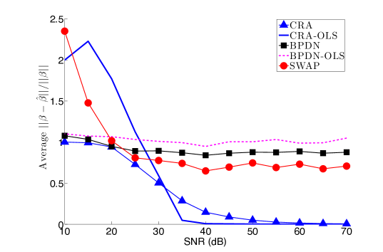
Figure 2. The average estimation error across different noise levels in the “synthetic data” experiment of Section 5.1. Each data point corresponds to the average estimation error over 30 realizations.

Figure 3 compares the true positive rate of the algorithms. As the figure suggests, CRA recovers most of the true support up until $30$ dB. Afterwards, the estimation quality falls significantly for all of the algorithms.

Figure 3. The true positive rate across different noise levels in the “synthetic data” experiment of Section 5.1. Each data point corresponds to the average true positive rate over 30 realizations.

The average running time of the algorithms, all on the same machine, are presented in Table 1. Empirically, we observe that SPGL1 solves the CRA problem, which does not have high correlation in it, much faster. Moreover both CRA and BPDN are considerably faster than SWAP.

Algorithm	Running Times (s)
CRA (without clustering)	0.044
clustering with eigenvectors	0.023
BPDN	0.730
SWAP	4.100

Table 1. Average running times of various algorithms over 570 trials (30 trials per noise level for 19 different values of $\sigma$) for the example presented in Section 5.1.

5.2. Pseudo-Real Data

5.2.1. The Data Description

For the purpose of the numerical simulations with real data, we consider daily stock prices. Daily stock prices present us with a real life data set with a complex high correlation environment. We use the prices of 2000 NASDAQ stocks recorded from June 15 2012 to June 15 2014. After removing the holidays, non-trading days, and special trading session, each stock has 500 observations. To give some structure to the data, we remove the trends from each time series, and also rescale the $l_{2}$ norm of each series to $\sqrt{n}$. After this stage, the data is used to populate the matrix $X\in\mathbb{R}^{500\times 2000}$. Figure 4 is the graphical representation of $\dfrac{1}{n}X^{*}X$. It is evident that, even after all modification on the data, $\dfrac{1}{n}X^{*}X$ is very different from identity, and hence $X$ does not fit into the category of suitable matrices for sparse recovery.

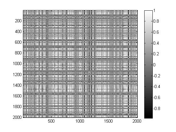
Figure 4. The matrix $\frac{1}{n}X^{*}X$.

5.2.2. Results

By using k-means clustering, we identify 14 clusters in the data, hence $R\in\mathbb{R}^{500\times 14}$. Figure 5 is the graphical representation of $\frac{1}{n}\left(\Pi_{R^{\perp}}XN_{\Pi_{R^{\perp}}X}^{-1}\right)^{*}\left(\Pi_{R^{\perp}}XN_{\Pi_{R^{\perp}}X}^{-1}\right)$. As we can see, we have a tremendous improvement in the covariance structure of the data matrix.

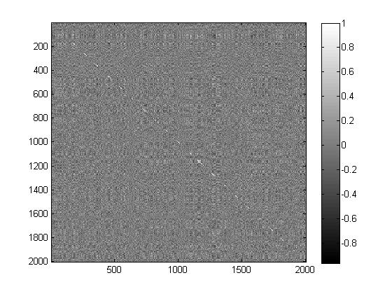
Figure 5. The covariance matrix of $\Pi_{R^{\perp}}XN_{\Pi_{R^{\perp}}X}^{-1}$

Figure 6 shows the singular values of $X$ on the left hand side, and singular values of $\widetilde{X}$ on the right. For comparison we include in the left figure the plot of the singular values of a $500\times 2000$ matrix with columns uniformly distributed on $S^{484}$. Although there is considerable difference between the singular values of $\widetilde{X}$ and those of the matrix with uniformly distributed columns, we observe a vast improvement compared to the original case. This improvement is in fact sufficient for us to successfully perform sparse estimation. One can choose more than 14 clusters or use a more advanced clustering method to make the singular values of $\widetilde{X}$ closer to the uniform case. However, we empirically observed that this does not improve the estimation results significantly.

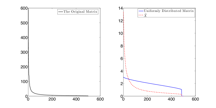
Figure 6. The SVD comparison of $\widetilde{X}$, $X$, and a uniformly distributed matrix in the “pseudo-real data” experiment of Section 5.2.

Figure 7 demonstrates the average value of $\dfrac{||\beta-\hat{\beta}^{\{20\}}||_{2}}{||\beta||_{2}}$ for all five algorithms. As Figure 7 shows, in low noise settings, CRA-OLS and CRA have the best performance among the algorithms. As the noise level increases, distinguishing between the columns of $X$ becomes almost impossible. For noise levels more than $20$ dB, none of the algorithms provide a reasonable estimate of $\beta$.

Figure 7. The average estimation error across different noise levels in the “pseudo-real data” experiment of Section 5.2. Each data point corresponds to the average estimation error over 30 realizations.

Figure 8 shows the average value of $\text{TPR}(\hat{\beta}^{\{20\}})$ across different noise levels, for each algorithm. It can be observed that again CRA outperforms both SWAP and BPDN.

Figure 8. The true positive rate across different noise levels in the “pseudo-real data” experiment of Section 5.2. Each data point corresponds to the average true positive rate over 30 realizations.

In SWAP, the sparsity rate of the final vector is always equal to the size of the initial support provided, $|T_{0}|$. To make sure that SWAP’s estimate has a high TPR ( although in the expense of adding false positive indices), [17] suggest providing a larger $T_{0}$. Indeed, our results suggest that if we allow SWAP to search for a 30-sparse vector in estimating a 20-sparse $\beta$, $\text{TPR}(\hat{\beta}_{SWAP})$ increases. However, as the size of the support that SWAP is working with increases, the running time of SWAP increases significantly. The following table represent the average running time of the algorithms on the same machine

Algorithm	Running Times (s)
BPDN	0.90
K-means Clustering	2.48
CRA (with Clustering)	3.70
SWAP (20-sparse)	18.57
SWAP (30-sparse)	146.27

Table 2. Average running times of various algorithms over 570 trials (30 trials per noise level for 19 different values of $\sigma$) for the example presented in Section 5.2.

A second point to consider is the sensitivity of the algorithm’s performance to the number of observations. We run the same experiment as above but we discard the first 250 observations so $X\in\mathbb{R}^{250\times 2000}$. Figure 9 shows the difference between the average TPR with 500 observations and the average TPR with 250 observations for each algorithm. In comparison to other algorithms, CRA’s performance falls much less when the number of observations decreases while SWAP’s performance degrades significantly.

Figure 9. The difference between the performances of each algorithm when the number of observations is reduced from 500 to 250.

6. Conclusions and Future Work

CRA is a computationally efficient estimation method that allows for sparse recovery in highly correlated environments. As we showed in Section 5, even with extremely simple clustering algorithms, CRA’s empirical performance is superior to other state-of-the-art sparse recovery algorithms. Moreover, CRA is computationally efficient (as reflected in the run times given in Tables 1 and 2) which makes it suitable for working with large data sets. In addition, the algorithm provides a large degree of flexibility in the choices of the sparse recovery technique and clustering method. Accordingly, CRA is a versatile sparse estimation method for cases where the design matrix (or equivalently, the compressive sensing measurement matrix) has correlated columns that can be grouped into a small number of clusters as we described before.

Despite all these strengths, there are certain setting where one may need to modify CRA. First, as we noted earlier, in noisy environments, as the data becomes more and more highly correlated, distinguishing the columns from each other becomes impossible. In this case, to decrease the correlation in the matrix, one might want to group the columns that are extremely correlated with each other and then run CRA on the representative vectors of the grouped variables. There are many approaches for variable grouping, e.g., [4] and [9] introduce two new automated grouping algorithms and provide a short survey of the field. Combining CRA with these variable grouping algorithms is an interesting subject for future research.

Another interesting problem is whether one can relax the rigid cluster structure imposed by our assumptions. This would mean that we adapt CRA for sparse recovery in the case of design matrices with correlated columns that do not satisfy our Assumptions 1-3.

7. Acknowledgements

B. Ghorbani was funded by a UBC Arts Summer Research Award and a UBC Arts Undergraduate Research Award. Ö. Yılmaz was funded in part by a Natural Sciences and Engineering Research Council of Canada (NSERC) Discovery Grant (22R82411), an NSERC Accelerator Award (22R68054) and an NSERC Collaborative Research and Development Grant DNOISE II (22R07504).

References

- [1] Jushan Bai and Serena Ng. Large dimensional factor analysis. Now Publishers Inc, 2008.
- [2] Alexandre Belloni and Victor Chernozhukov. Least squares after model selection in high-dimensional sparse models. Bernoulli, 19(2):521–547, 05 2013.
- [3] Thomas Blumensath and Mike E Davies. Iterative thresholding for sparse approximations. Journal of Fourier Analysis and Applications, 14(5-6):629–654, 2008.
- [4] P. Bühlmann, P. Rütimann, S. van de Geer, and C.-H. Zhang. Correlated variables in regression: clustering and sparse estimation. ArXiv e-prints, September 2012.
- [5] T.T. Cai and Anru Zhang. Sparse representation of a polytope and recovery of sparse signals and low-rank matrices. Information Theory, IEEE Transactions on, 60(1):122–132, Jan 2014.
- [6] Emmanuel J. Candès, Justin K. Romberg, and Terence Tao. Stable signal recovery from incomplete and inaccurate measurements. Communications on Pure and Applied Mathematics, 59(8):1207–1223, 2006.
- [7] Jens Peter Reus Christensen. On some measures analogous to haar measure. Mathematica Scandinavica, 26:103–106, 1970.
- [8] D.L. Donoho, M. Elad, and V.N. Temlyakov. Stable recovery of sparse overcomplete representations in the presence of noise. Information Theory, IEEE Transactions on, 52(1):6–18, Jan 2006.
- [9] Mario AT Figueiredo and Robert D Nowak. Sparse estimation with strongly correlated variables using ordered weighted l1 regularization. arXiv preprint arXiv:1409.4005, 2014.
- [10] S. Foucart. Hard thresholding pursuit: An algorithm for compressive sensing. SIAM Journal on Numerical Analysis, 49(6):2543–2563, 2011.
- [11] Matthew A Herman and Thomas Strohmer. General deviants: An analysis of perturbations in compressed sensing. Selected Topics in Signal Processing, IEEE Journal of, 4(2):342–349, 2010.
- [12] Deanna Needell and Joel A Tropp. Cosamp: Iterative signal recovery from incomplete and inaccurate samples. Applied and Computational Harmonic Analysis, 26(3):301–321, 2009.
- [13] Robert Tibshirani. Regression shrinkage and selection via the lasso. Journal of the Royal Statistical Society. Series B (Methodological), pages 267–288, 1996.
- [14] J.A Tropp and AC. Gilbert. Signal recovery from random measurements via orthogonal matching pursuit. Information Theory, IEEE Transactions on, 53(12):4655–4666, Dec 2007.
- [15] E. van den Berg and M. P. Friedlander. SPGL1: A solver for large-scale sparse reconstruction, June 2007. http://www.cs.ubc.ca/labs/scl/spgl1.
- [16] E. van den Berg and M. P. Friedlander. Probing the pareto frontier for basis pursuit solutions. SIAM Journal on Scientific Computing, 31(2):890–912, 2008.
- [17] Divyanshu Vats and Richard G Baraniuk. Swapping variables for high-dimensional sparse regression from correlated measurements. arXiv preprint arXiv:1312.1706, 2013.
- [18] Roman Vershynin. Introduction to the non-asymptotic analysis of random matrices. arXiv preprint arXiv:1011.3027, 2010.
- [19] John Wright and Yi Ma. Dense error correction via-minimization. Information Theory, IEEE Transactions on, 56(7):3540–3560, 2010.