The relationship between a strip Wiener–Hopf problem and a line Riemann–Hilbert problem

Abstract.

In this paper the Wiener–Hopf factorisation problem is presented in a unified framework with the Riemann–Hilbert factorisation. This allows to establish the exact relationship between the two types of factorisation. In particular, in the Wiener–Hopf problem one assumes more regularity than for the Riemann–Hilbert problem. It is shown that Wiener–Hopf factorisation can be obtained using Riemann–Hilbert factorisation on certain lines.

1. Introduction

The Wiener–Hopf and the Riemann–Hilbert problems are a subject of many books and articles [Ehr_spit, Ehr_Spec, Constructive_review, Spit, Camara_2]. The similarities of the two techniques are easily visible and have been noted in many places. Nevertheless, to the author’s knowledge there was no systematic study of the exact relationship of the two methods. To fill this gap is the purpose of this article.

It has been suggested in [bookWH, Chapter 4.2] that the Wiener–Hopf equation are a special case of a Riemann–Hilbert equation. Specifically, the Riemann–Hilbert problem connects boundary values of two analytic functions on a contour and the Wiener–Hopf equation is defined on the strip of common analyticity of two functions. In the simplest case, both methods use the key concept of functions analytic in half-planes. The additional regularity for the Wiener–Hopf equation allows to express the solution in more simple terms than the Riemann–Hilbert equation. To be well-defined the Riemann–Hilbert problem requires some additional regularity, e.g. the coefficients need to be Hölder continuous on the contour.

In a different book [Ga-Che, Chapter 14.4] it has been stated that the Wiener–Hopf equations results from a bad choice of functions spaces and instead a Riemann–Hilbert equations should be considered. Confusingly, those Riemann–Hilbert equations are sometimes referred to as a Wiener–Hopf equations. Historically, there has been insufficient interaction between the communities using the Wiener–Hopf and the Riemann–Hilbert methods, this results in obscuring disagreements in terminology and notations. Such differences if not reconciled properly have a tendency to widen.

We consider the following problem as an illustration. Given a function $F(t)$ on the real axis:

$$F(t)=\sqrt{\frac{t^{2}-(\frac{1}{2}i+1)t-\frac{1}{4}i+\frac{3}{4}}{t^{2}-\frac{3}{2}it+1}}\frac{(t-i+2)}{(t+i+\frac{3}{2})},$$ (1.1)

find two factors $F^{+}(t)$ and $F^{-}(t)$, which have analytic extensions in the upper and lower half-planes respectively. In this rare case the factorisation can be obtained by inspection

$$F(t) =\left(\sqrt{\frac{(t+\frac{1}{2}i-\frac{1}{2})}{(t+\frac{1}{2}i)}}\frac{1}{(t+i+\frac{3}{2})}\right)\times\left(\sqrt{\frac{(t-i-\frac{1}{2})}{(t-2i)}}(t-i+2)\right)$$

$$=F^{+}(t)F^{-}(t).$$ (1.2)

These functions are depicted in Figure 1. We will comment on this example in both (the Riemann–Hilbert and Wiener–Hopf) frameworks at the end of this paper.

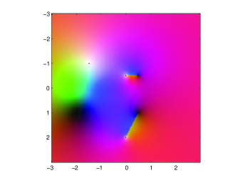
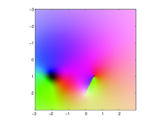
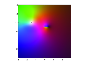
Figure 1. A full colour image of functions (1.2). The top picture shows $F(z)$ followed by $F^{+}(z)$ and $F^{-}(z)$. We use a colour scheme developed by John Richardson. Red is real, blue is positive imaginary, green is negative imaginary, black is small magnitude and white is large magnitude. Branch cuts appear as colour discontinuities. Produced using MATLAB package zviz.m.

The structure of the paper is as follows. Section 2 collects some preliminaries. In Section 3, the usual theoryoptx and applications of the Wiener–Hopf equation is recalled. It is presented to highlight the differences with the theory of the Riemann–Hilbert equations, Section 4. Section 5 describes at the relationship between the two methods in the context of integral equations. In Section 6 the solution to Wiener–Hopf and Riemann–Hilbert factorisation is re-expressed in terms of the Fourier transforms instead of the Cauchy type integrals. This allows to prove theorems about the exact relationship of Wiener–Hopf and Riemann–Hilbert factorisation.optx The last section gives some interesting historical remarks.

2. Preliminaries

This section will review important properties of the Fourier transform, the Cauchy type integral and the relationship between the two. We also states the generalised version of Liouville’s Theorem together with analytic continuation, in the form which will be used later.

The Fourier transform of a function $f(t)$ is defined as

$$F(x)=\frac{1}{\sqrt{2\pi}}\int\limits_{-\infty}^{\infty}f(t)e^{ixt}dt,\quad-\infty<x<\infty.$$ (2.1)

Throughout this paper the Fourier image and original function will be denoted by the same letter but they will be upper and lower case respectively. The inverse Fourier transform is given:

$$f(t)=\frac{1}{\sqrt{2\pi}}\int\limits_{-\infty}^{\infty}F(x)e^{-ixt}dt,\quad-\infty<t<\infty.$$

It is an important fact that if $f(t)\in L_{2}(\mathbb{R})$ then $F(t)\in L_{2}(\mathbb{R)}$. This makes the space of square integrable functions very convenient to work in. Moreover, Fourier transform is an isometry of $L_{2}(\mathbb{R)}$ due to Plancherel’s theorem.

The Fourier transform need not be confined to the real axis, as long as the integral (2.1) is absolutely convergent for a complex $x$. On an open domain consisting of such parameters $x$, the Fourier transform is an analytic function. The Paley–Wiener theorem (see (2.6)–(2.8) below) gives the conditions on the decay at infinity of $f(t)$ to ensure such analyticity in different strips and half-planes.

Another key concept is the Cauchy type integral. Let $F(\tau)$ be integrable on a simple Jordan curve $L$, the integral

$$\frac{1}{2\pi i}\int_{L}\frac{F(\tau)}{\tau-z}d\tau,$$

is called a Cauchy type integral and defines an analytic function on the complement of $L$. If $L$ divides the complex plane into two disjoint open components then it makes sense to consider two functions $F^{-}$ and $F^{+}$ on the respective domains. In particular, for the real line we use the notation:

$$\frac{1}{2\pi i}\int\limits_{-\infty}^{\infty}\frac{F(\tau)}{\tau-z}d\tau=\left\{\begin{array}[]{rl}F^{+}(z)&\text{if }\mathrm{Im}\,z>0,\\ F^{-}(z)&\text{if }\mathrm{Im}\,z<0.\\ \end{array}\right.$$ (2.2)

The relationship of the Cauchy type integral to the Fourier transform is outlined below.

$$\frac{1}{2\pi i}\int\limits_{-\infty}^{\infty}\frac{F(\tau)}{\tau-z}d\tau =\frac{1}{\sqrt{2\pi}}\int\limits_{0}^{\infty}f(t)e^{izt}dt\,, \text{if }\mathrm{Im}\,z>0,$$ (2.3)

$$\frac{1}{2\pi i}\int\limits_{-\infty}^{\infty}\frac{F(\tau)}{\tau-z}d\tau =-\frac{1}{\sqrt{2\pi}}\int\limits_{-\infty}^{0}f(t)e^{izt}dt\,, \text{if }\mathrm{Im}\,z<0.$$ (2.4)

The above integrals are the two ways of arriving at functions analytic in half-planes.

It was already mentioned that $L_{2}(\mathbb{R})$ is a very convenient with regards to the Fourier transform. The Hölder continuous functions produce well-defined boundary values of the Cauchy integral. Thus, their intersection [Ga-Che]*§ 1.2:

$$\{\!\{0\}\!\}=L_{2}(\mathbb{R})\cap\text{ H\"{o}lder},$$

turns out to be very useful for both the Wiener–Hopf and the Riemann–Hilbert problems. The pre-image of $\{\!\{0\}\!\}$ under the Fourier transform is denoted $\{0\}$.

Formulae (2.3)–(2.4) show the significance of functions which are zero on the positive or the negative half lines. Given a function on the real axis we can define the splitting

$$f_{+}(t)=\left\{\begin{array}[]{rl}f(t)&\text{if }t>0,\\ 0&\text{if }t<0,\\ \end{array}\right.\quad f_{-}(t)=\left\{\begin{array}[]{rl}0&\text{if }t>0,\\ -f(t)&\text{if }t<0.\\ \end{array}\right.$$ (2.5)

We will say that if $f\in\{0\}$ then $f_{+}(t)\in\{0,\infty\}$ and $f_{-}(t)\in\{-\infty,0\}$.

In the rest of the paper we will need to refer to functions that are analytic on strips or (shifted) half-planes. Following [Ga-Che]*§ 13, we define $f\in\{a\}$ if $e^{-ax}f\in\{0\}$, that is a shift in the Fourier space. Finally, $f=f_{+}+f_{-}\in\{a,b\}$ if $f_{+}\in\{a\}$ and $f_{-}\in\{b\}$. From the definition of $f_{+}$ and $f_{-}$ it is clear that also $f_{+}\in\{a,\infty\}$ and $f_{-}\in\{-\infty,b\}$.

The Fourier transform of functions in the class $\{a,b\}$ is denoted $\{\!\{a,b\}\!\}$. The celebrated Paley–Wiener theorem states that the following is equivalent :

$$F_{+}(z)\text{ analytic in Im}z>a \iff F_{+}(z)\in\{\!\{a,\infty\}\!\},$$ (2.6)

$$F_{-}(z)\text{ analytic in Im}z<b \iff F_{-}(z)\in\{\!\{-\infty,b\}\!\},$$ (2.7)

$$F(z)\text{ analytic in }a<\mathrm{Im}\,z<b \iff F(z)\in\{\!\{a,b\}\!\}.$$ (2.8)

Recall, a convolution of two functions on the real line is given by

$$h(t)=\frac{1}{2\pi i}\int\limits_{-\infty}^{\infty}f(t-s)g(s)\,ds.$$ (2.9)

One of the key properties, which make Fourier techniques useful in integral equations, is that the Fourier transform of the convolution is the product of the Fourier transform of the functions $f(t)$ and $g(t)$, i.e. $H(x)=F(x)G(x)$.

If $g\in\{a,b\}$ and $f\in\{\alpha,\beta\}$ ($a<b$, $\alpha<\beta$) then $h(x)$ will be in the class $\{\text{max}(a,\alpha),\text{min}(b,\beta)\}$ [Ga-Che]*§ 1.3 provided

$$\text{max}(a,\alpha)<\text{min}(b,\beta).$$

After taking the Fourier transform this will become:

$$H(z)=F(z)G(z),$$

and $H(z)\in\{\!\{\text{max}(a,\alpha),\text{min}(b,\beta)\}\!\}$ i.e analytic in the strip

$$\text{max}(a,\alpha)<\mathrm{Im}\,(z)<\text{min}(b,\beta).$$ (2.10)

We will need a generalised version of Liouville’s Theorem together with analytic continuation:

Theorem 2.1 ([Ga-Che]*§ 3.1).

If functions $F_{1}(z)$, $F_{2}(z)$ are analytic in the upper and lower half-planes respectively with exception of $z_{0}=\infty,$ $z_{k}$ ($k=1,2\dots n$) where they have poles with principal parts:

$$G_{0}(z) = c_{1}^{0}z+\dots c_{m_{0}}^{0}z^{m}_{0},$$ (2.11)

$$G_{k}\left(\frac{1}{z-z_{k}}\right) = \frac{c_{1}^{k}}{z-z_{k}}+\dots\frac{c_{m_{k}}^{k}}{(z-z_{k})^{m_{k}}},$$ (2.12)

with $F_{1}(z)$ and $F_{2}(z)$ equal on the real axis, then they define a rational function on the whole plane:

$$F(z)=c+G_{0}(z)+\sum_{1}^{n}G_{k}\left(\frac{1}{z-z_{k}}\right),$$

where $c$ is an arbitrary constant. Poles $z_{k}$ can lie anywhere on the half-planes or on the real axis.

3. The Wiener–Hopf Method

In this section the Wiener–Hopf method is presented in the way it appears in most papers. This will be revisited to establish the relationship with the Riemann–Hilbert method. optaFor some applications of Wiener-Hopf in areas like elasticity, crack propagation and acoustics see [Mishuris-Rogosin, owl, Abr_clam, Nigel_cyl].

optx Wiener–Hopf is an elegant method based on the exploitation of the analyticity properties of the functions [bookWH]*Ch. 1. The first step of the method is to reduce the governing partial differential equation to an ordinary differential equation (ODE) via the Fourier transform. By using the ODE and the boundary conditions a Wiener–Hopf equation is obtained. The resulting equation is analytic in a strip, which mostly contains the real line, and has two unknown functions. Then the key step is to obtain a factorisation such that the right side of the equation is analytic in the upper half-plane and the strip, and the left side is analytic in the lower half-plane and the strip. Through the use of analytic continuation and Liouville’s Theorem two separate equations are obtained with one unknown function each. These can now be solved and mapped back to the original set-up using the inverse Fourier transform.

The following conventions will be used throughout the section:

• A strip around the real axis (given $\tau_{-}<0<\tau_{+}$) is {$\alpha=\sigma+i\tau$ : $\tau_{-}<\tau<\tau_{+}$}$\subset\mathbb{C}$.
  

• The subscript $+$ (or $-$) indicates that the function is analytic in the half-plane $\tau>\tau_{-}$ (or $\tau<\tau_{+}$).
  

• Functions in the Wiener–Hopf equation without the subscript are analytic in the strip.
  

The Wiener–Hopf problems are recalled below.

The multiplicative Wiener–Hopf problem is: given a function $K$ (analytic, zero-free and $K(\alpha)\to 1$ as $|\sigma|\to\infty$ in the strip) to find functions $K_{+}$ and $K_{-}$ which satisfy the following equation in the strip:

$$K(\alpha)=K_{-}(\alpha)K_{+}(\alpha).$$ (3.1)

In addition $K_{-}$ and $K_{+}$ are required to be:

• analytic and non-zero in the respective half-plane.

• of subexponential growth the respective half-planes:

  $$|\log K_{\pm}(\alpha)|=O(|\alpha|^{p}),\quad p<1,\quad\text{as}\quad|\sigma|\to\infty.$$

The function $K(\alpha)$ in the multiplicative Wiener–Hopf factorisation will be referred to as the kernel. The functions $K_{+}$ and $K_{-}$ will be called factors of $K$.

optxThe multiplicative Wiener–Hopf factorisation can be reduced to the additive Wiener–Hopf problem via application of logarithm. Under the conditions on the kernel $K$, let $f=\log K$ then additive Wiener–Hopf problem is: given a function $f$, find functions $f_{+}$ and $f_{-}$ which satisfy the following equation in the strip:

$$f(\alpha)=f_{-}(\alpha)+f_{+}(\alpha).$$ (3.2)

Additive and multiplicative problems are equivalent only in the scalar case. In the matrix Wiener–Hopf $K_{+}$ and $K_{-}$ will in general not be commutative so no such equivalence is possible.

The existence of solutions to the additive and multiplicative scalar Wiener–Hopf problem is addressed in Section LABEL:subsec:exact.

optx

3.1. The Wiener–Hopf Procedure

The discussion in this section is based on the book by Noble  [bookWH]. This book is a brilliant introduction to the topic and contains numerous examples of the problems which can be solved as well as a discussion of the difficulties faced.

The Wiener–Hopf problem is to find the unknown functions $\Phi_{+}$ and $\Psi_{-}$ which satisfy the following equation in a strip around the real axis:

$$A(\alpha)\Phi_{+}(\alpha)+\Psi_{-}(\alpha)+C(\alpha)=0.$$

The key step in the Wiener Hopf procedure is to find invertible $K_{+}$ and $K_{-}$ (the Wiener–Hopf factors) such that:

$$A(\alpha)=K_{+}(\alpha)K_{-}(\alpha).$$

The product of functions analytic in the respective half planes will be refereed to as a factorisation of the kernel.

Then multiplying though:

$$K_{+}\Phi_{+}(\alpha)+K_{-}^{-1}\Psi_{-}(\alpha)+K_{-}^{-1}C(\alpha)=0.$$

Now splitting additively:

$$K_{-}^{-1}C(\alpha)=C_{-}(\alpha)+C_{+}(\alpha).$$

Finally rearranging the equation:

$$K_{+}\Phi_{+}(\alpha)+C_{+}(\alpha)=-K_{-}^{-1}\Psi_{-}(\alpha)-C_{-}(\alpha).$$

The right hand side is a function analytic in $\tau>\tau_{-}$ and the left in $\tau<\tau_{+}$. So by analytic continuation (from the strip) define a function $J(\alpha)$ analytic everywhere in the complex plane. The requirement on the equation is that there exists an $n$ such that (at most polynomial growth):

$$J(\alpha)<|\alpha|^{n}\quad|\alpha|\to\infty.$$

Applying the extended Liouville’s theorem to $J(\alpha)$ implies that $J(\alpha)$ is a polynomial of degree less than or equal to $n$. So the solution is reduced to finding $n$ unknown constants which can be determined in some other way (typically $n=0$ or $1$). Hence $\Phi_{+}(\alpha)$ and $\Psi_{-}(\alpha)$ are determined.

There are a few issues which determine whether the method will work or not. The first is finding $K_{+}$ and $K_{-}$. The second is to find $C_{-}(\alpha)$ and $C_{+}(\alpha)$ which will turn out to be similar to the first part. Lastly the resulting function can have at most polynomial growth.

Remark 3.1.

The equation does not have to hold in the strip $\tau_{-}<\tau<\tau_{+}$ the above method works as long as there is strip which for $\sigma$ large enough includes the real line. Typically the strip is deformed around singularities.

Remark 3.2.

In the same way the following equation could be considered:

$$A(\alpha)\Phi_{+}(\alpha)+B(\alpha)\Psi_{-}(\alpha)+C(\alpha)=0.$$

As long as $B(\alpha)$ is invertible.

Remark 3.3.

The same works for matrix valued functions provided the factorisation is found.

opta For details on the fascinating history of Wiener–Hopf see [history].

The next theorem provides a constructive existence theorem for the additive Wiener–Hopf decomposition (in terms of a Cauchy type integral).

Theorem 3.4 ([bookWH]*Ch. 1.3).

Let $f(\alpha)$ be a function of variable $\alpha=\sigma+i\tau$, analytic in the strip $\tau_{-}<\tau<\tau_{+}$, such that $f(\sigma+i\tau)<C|\sigma|^{-p}$, $p>0$ as $|\sigma|\to\infty$, the inequality holding uniformly for all $\tau$ in the strip $\tau_{-}+\epsilon<\tau<\tau_{+}-\epsilon,$ $\epsilon>0$. Then for $\tau_{-}<c<\tau<d<\tau_{+},$

$$f(\alpha)=f_{-}(\alpha)+f_{+}(\alpha),$$

$$f_{-}(\alpha)=-\frac{1}{2\pi i}\int\limits_{-\infty+id}^{\infty+id}\frac{f(\zeta)}{\zeta-\alpha}d\zeta\quad;\quad f_{+}(\alpha)=\frac{1}{2\pi i}\int\limits_{-\infty+ic}^{\infty+ic}\frac{f(\zeta)}{\zeta-\alpha}d\zeta,$$ (3.3)

where $f_{-}$ is analytic in $\tau<\tau_{+}$ and $f_{+}$ is analytic in $\tau>\tau_{-}$.

We wish to highlight the simplicity of demonstration of this result. Indeed, to prove (3.3) one applies Cauchy’s integral theorem to the rectangle with vertices $\pm a+ic$, $\pm a+id$. From the assumption as regards to the behaviour of $f(\alpha)$ as $|\sigma|\to\infty$ in the strip, the integral on $\sigma=\pm a$ tends to zero as $a\to\infty$ and the result follows.

The next theorem is a useful variation of the previous theorem, obtained by taking logarithms. This provides a way to achieve the multiplicative Wiener–Hopf factorisation.

Theorem 3.5.

[bookWH]*Ch. 1.3 If $\log K$ satisfies the conditions for theorem 3.4 in particular that $K(\alpha)$ is analytic and non-zero in the strip and $K(\alpha)\to 1$ as $|\sigma|\to\infty$ then $K(\alpha)=K_{+}(\alpha)K_{-}(\alpha)$ and $K_{+}$, $K_{-}$ are analytic, bounded and non-zero when $\tau>\tau_{-}$, $\tau<\tau_{+}$ respectively.

The above factors are unique up to a constant [Kranzer_68]. In other words, if there are two such factorisations $K=K_{+}K_{-}$ and $K=P_{+}P_{-}$, then:

$$K_{+}=cP_{+}\quad\text{and}\quad K_{-}=c^{-1}P_{-},$$

where $c$ is some complex constant. This can be seen by applying analytic continuation to $K_{+}/P_{+}$ and $P_{-}/K_{-}$ and then using the extended Liouville theorem 2.1.

optx

3.2. Application to PDEs

In this section it is shown how PDEs with semi-infinite boundary conditions can be reduced to the Wiener–Hopf equation. There are a lot of different applications in areas like elasticity, crack propagation and acoustics [Mishuris-Rogosin, owl, Abr_clam].

Below are some properties of the half space Fourier transform which will be needed to arrive at an equation of the form in the previous subsection. The following properties will be needed:

$$F_{+}(\alpha)=\int\limits_{0}^{\infty}f(x)e^{i\alpha x}dx,$$

and

$$F_{-}(\alpha)=\int^{0}_{-\infty}f(x)e^{i\alpha x}dx.$$

In other words $F_{+}(\alpha)$ is analytic in the upper half plane and $F_{-}(\alpha)$ is analytic in the lower half plane; this is true if:

• $f(\xi)$ has a finite number of discontinuities on the real line, has finite number of maxima and minima on any interval

• $f(\xi)$ is bounded except at the finite number of points and the limit of $\int f(\xi)$ on the deformed contour as the deformation tends to the real line exists.

In our case the above will always be satisfied.

The first example of such PDE comes from acoustics. Consider the boundary value problem governed by the reduced wave equation:

$$\left(\frac{\partial}{\partial x^{2}}+\frac{\partial}{\partial y^{2}}+c^{2}\right)\phi(y,x)=0,\quad\text{with}\quad c\in\mathbb{R},$$

and in the semi-infinite region $-\infty<x<\infty$, $y\geq 0$ with boundary conditions:

$$\phi = f(x)\quad\text{on}\quad y=0\qquad 0<x<\infty,$$ (3.4)

$$\frac{\partial\phi}{\partial y} = g(x)\quad\text{on}\quad y=0\quad-\infty<x<0.$$ (3.5)

Define half-range and full-range Fourier transforms:

$$\Phi(y,\alpha)= \int\limits_{-\infty}^{0}\phi(y,\xi)e^{i\alpha\xi}d\xi+\int^{\infty}_{0}\phi(y,\xi)e^{i\alpha\xi}d\xi,$$ (3.6)

$$= \Phi_{-}(y,\alpha)+\Phi_{+}(y,\alpha),$$ (3.7)

Taking the Fourier transform of the reduced wave equation gives:

$$\frac{d\Phi(y,\alpha)}{dy^{2}}-(\alpha^{2}-c^{2})\Phi(y,\alpha)=0.$$

Now solving the ODE:

$$\Phi(y,\alpha)=A(\alpha)e^{-\gamma y}\quad\text{where}\quad\gamma(\alpha)=\sqrt{\alpha^{2}-c^{2}}$$

imposing a restriction of polynomial growth as $y\to\infty$.

The taking the Fourier transform of the boundary conditions yield:

$$\Phi_{+}(0,\alpha)+\Phi_{-}(0,\alpha)=A(\alpha),\qquad\Phi^{\prime}_{+}(0,\alpha)+\Phi^{\prime}_{-}(0,\alpha)=-\gamma(\alpha)A(\alpha).$$

Note that the functions $\Phi^{\prime}_{-}(0,\alpha)$ and $\Phi_{+}(0,\alpha)$ are unknown while the other two are given by the boundary conditions.

Now eliminating $A(\alpha)$ gives a Wiener–Hopf equation:

$$-\gamma(\alpha)\{\Phi_{+}(0,\alpha)+\Phi_{-}(0,\alpha)\}=\Phi^{\prime}_{+}(0,\alpha)+\Phi^{\prime}_{-}(0,\alpha).$$

This can now be solved using the Wiener–Hopf procedure; in other words $\Phi^{\prime}_{-}(0,\alpha)$ and $\Phi_{+}(0,\alpha)$ can be determined. This allows the $A(\alpha)$ to be calculated and hence $\Phi(y,\alpha)$. Taking the inverse Fourier transform of $\Phi(y,\alpha)$ gives the required solution to the PDE.

3.3. Random Matrix Theory and Interacting Particles

This section demonstrates the variety of applications of the Wiener–Hopf method and illustrates the connection to stochastic processes. For this purpose the background of the derivation of the Wiener–Hopf equation is discussed. But since the actual solution of the equation is not of importance here it will be omitted.

We will explore the fascinating relationship between random matrices, diffusion processes, interacting particles, McKean-Vlasov equations and the Wiener–Hopf type equation. The material presented here is taken from two paper by Chan (1992) and (1994) [dif1] and [dif2].

All of this is partly motivated by the beautiful result called the Wigner semicircle law. Consider a random symmetric matrix with i.i.d. entries normally distributed with mean 0 and variance $\sigma^{2}n^{-1}$. Then the result states that the density of eigenvalues of the matrix will be tending to a semi circle with density:

$$\frac{\sqrt{4\sigma^{2}-y^{2}}}{2\pi\sigma^{2}},\quad|y|\leq 2\sigma.$$

This result is not just a curious phenomena this result is important in the statistical theory of energy levels. In this setting the random symmetric matrix is the finite dimensional approximation to the Hamiltonian. In the consideration of the Schrödinger equation the eigenvalues play a big role hence the application of this result. To clarify the nature of this elegant result we will be considering symmetric matrices with entries diffusion processes in particular the Ornstein-Uhlenberck processes.

Let $X_{t}$ be a symmetric $n\times n$ matrix process evolving according to Ornstein-Uhlenberck:

$$dX=-\frac{1}{2}Xdt+\frac{1}{2\sqrt{n}}(dB+dB^{T}),$$

where $B$ is standard matrix valued Brownian motion and $B^{T}$ its transpose. It is important to note that this process has normal distribution as invariant measure.

Now if we consider the evolution of eigenvalues of this matrix we will find that they satisfy:

$$d\lambda_{i}=\frac{1}{\sqrt{n}}dB_{i}-\frac{1}{2}\lambda_{i}dt+\frac{1}{2n}\sum_{k\neq i}\frac{1}{\lambda_{i}-\lambda_{k}}dt,\quad i=1,\dots,n.$$

where $B_{i}$ are independent Brownian motions in $\mathbb{R}$. This can be derived using Itô’s calculus and the invariance of d$B$ under $O(n)$. This can also be interpreted as a system of $n$ particles interacting. More precisely we can think of it as $n$ charged particles in a single-well quadratic potential and interacting via electrostatic repulsion with some random element.

We will be interested in time evolution of a large number of particles. In particular, the associated measure valued process:

$$\mu_{n}(t)=\frac{\sum_{i=1}^{n}\delta_{\lambda_{i}(t)}}{n},$$

where $\delta_{y}$ denotes a point mass at $y$. We note that the flow of measure is non-linear and highly singular. Nevertheless it has been shown that $\mu_{n}(t)$ converges to a deterministic measure-valued function $\mu_{t}$. What is more it can be shown that if $\mu_{t}$ has no atomic component, then $\mu_{t}$ is the weak solution of the McKean-Vlasov equation:

$$\frac{d}{dt}\int\phi(\lambda)\mu_{t}(d\lambda)=\frac{1}{2}\int\left(\int\frac{\mu_{t}(dy)}{\lambda-y}-\lambda\right)\phi^{\prime}(\lambda)\mu_{t}(d\lambda),$$

for the suitable test functions $\phi$, one such choice would be to take $\phi_{\theta}(\lambda)=e^{-i\theta\lambda}$, $\theta\in\mathbb{R}$. Note that the integral in the bracket is the Cauchy principle value.

It has been shown by Chan that the Wigner semi circle density (with $\sigma=\sqrt{(}2)/2$) is the unique equilibrium point of the McKean-Vlasov equation under the regularity conditions of having Hölder-continuous density and belonging to $L^{2}$. Additionally if $\mu_{0}$ possesses finite moments of all order then $\mu_{t}$ actually tends to the semi circle density.

But there are difficulties in analysing the flow of measure $\mu_{t}$ using the McKean-Vlasov equation. They are only a weak solution so there is always the business of considering appropriate test functions. Below we describe a way to get around this problem.

We set the test functions to be $\phi_{\theta}(\lambda)=e^{-i\theta\lambda}$, $\theta\in\mathbb{R}$. Then the Fourier transform of $\mu$ called $\nu$ will satisfy the following integral Wiener–Hopf type equation:

$$\frac{\partial\nu}{\partial t}=\frac{\theta}{4}\left(\int\limits_{-\infty}^{0}\nu_{t}(u)\nu_{t}(\theta-u)du-\int^{\infty}_{0}\nu_{t}(u)\nu_{t}(\theta-u)du\right)-\frac{\theta}{2}\frac{\partial\nu}{\partial\theta},$$

where:

$$\nu_{t}(\theta)=\int_{-\infty}^{\infty}e^{-i\theta\lambda}\mu_{t}(d\lambda).$$

The study of this equation will help to clarify the semi circle law. This concludes this section which hopefully demonstrated some deep links that the Wiener–Hopf equation may offer.

4. The Riemann–Hilbert Method

In this section the main differences from the Wiener–Hopf method are presented.optx The same procedure as in Subsection 3.1 follows for the Riemann–Hilbert equation. They are rooted in the conditions imposed on the functions and the resulting formula. For applications of the Riemann–Hilbert problem the interested reader is refereed to [Fokas_Painleve, Gah].

The Riemann–Hilbert Problem can be stated as follows:

Problem 4.1 (Riemann–Hilbert).

On the real line two functions are given, $H(t)$ and non-zero $D(t)$ with

$$D(t)-1\in\{\!\{0\}\!\}\qquad\text{ and }\qquad H(t)\in\{\!\{0\}\!\}.$$

It is required to find two functions $F^{\pm}(z)$ analytic in the upper and lower half-planes such that their boundary values $F^{\pm}(t)$ on the real line satisfy two conditions:

1. $F^{\pm}(t)$ belong to the classes $\{\!\{0,\infty\}\!\}$ and $\{\!\{-\infty,0\}\!\}$;

2. The identity holds:

   $$D(t)F^{-}(t)+H(t)=F^{+}(t),\qquad\text{for all real }t.$$ (4.1)

As it has been seen for the Wiener–Hopf method the key steps in the solution is the additive splitting or jump problem (Thm. 3.4) and the factorisation (Thm. 3.5). First splitting is addressed as before:

Problem 4.2 (Jump problem).

On the real line a function $F(t)\in\{\!\{0\}\!\}$ is given. It is required to find two functions $F^{\pm}(z)$ analytic in the upper and lower half-planes with boundary functions on the real line belonging to the classes $\{\!\{0,\infty\}\!\}$ and $\{\!\{-\infty,0\}\!\}$ and satisfying:

$$F(t)=F^{+}(t)+F^{-}(t),$$

on the real line.

The solution is offered by the Sokhotskyi–Plemelj formula:

$$F^{+}(x)-F^{-}(x)=F(x),\qquad F^{+}(x)+F^{-}(x)=\frac{1}{\pi i}\int\limits_{-\infty}^{\infty}\frac{F(\tau)}{\tau-x}\,d\tau.$$ (4.2)

We shall note, that the derivation of (4.2) is more involved than the proof of Thm. 3.4.

Next the factorisation problem is examined. The index of a continuous non-zero function $K(t)$ on the real line is:

$$\mathrm{ind}(K(t))=\frac{1}{2\pi}\big{(}\lim_{t\to+\infty}\arg K(t)-\lim_{t\to-\infty}\arg K(t)\big{)}.$$ (4.3)

In other words the index is the winding number of the curve $(\text{Re }K(t),\mathrm{Im}\,K(t))$ $t\in\mathbb{R}$. Note that $\mathrm{ind}\,\frac{t-i}{t+i}=1.$ Given a function $K(t)$ with index $\kappa$ one can reduce it to zero index by considering a new function

$$K_{0}(t)=K(t)\left(\frac{t-i}{t+1}\right)^{-\kappa}.$$

The reason it is important to consider functions $K(t)$ with zero index is to ensure $\ln K(t)$ is single-valued. For the rest of this paper we will assume that all functions have zero index. Taking logarithms and applying the Sokhotskyi–Plemelj formula we get a solution to the factorisation problem [Ga-Che]:

Problem 4.3 (Riemann–Hilbert Factorisation).

Let a non-zero function $K(t)$, such that $K(t)-1\in\{\!\{0\}\!\}$ and $\mathrm{ind}\,K(t)=0$, be given. It is required to find two functions $K^{\pm}(z)$ analytic in the upper and lower half-planes with boundary functions $K^{\pm}(t)$ on the real line belonging to the classes $\{\!\{0,\infty\}\!\}$ and $\{\!\{-\infty,0\}\!\}$ and satisfying:

$$K(t)=K^{+}(t)K^{-}(t),$$

on the real line.

optx We can normalise so that $K_{\pm}(t)\to 1$ for $t\to\pm\infty$. The Riemann–Hilbert problem will be returned to in Section 6.

5. Relationship Between Wiener-Hopf and Riemann-Hilbert via Integral Equations

This section demonstrates how one type of integral equation can either lead to the Wiener–Hopf problem or the Riemann–Hilbert problem, depending on the class of function where the solution is sought. Integral equations have historically motivated the introduction of the Wiener–Hopf equation [history]optx, see Section LABEL:sec:his.

In applications, a time-invariant process can be modelled by an integral equations with convolution on the half-line:

$$\int\limits_{0}^{\infty}k(x-y)f(y)\,dy=g(x),\quad 0<x<\infty.$$ (5.1)

Here the kernel $k(x-y)\in\{a,b\}$ represents the process, $g(x)$ is a given output and $f(y)$ is an input to be determined. To solve the equation (5.1) we complement the domain of $x$:

$$\int\limits_{0}^{\infty}k(x-y)f(y)dy=h(x),\quad-\infty<x<0,$$ (5.2)

where $h(x)$ is unknown. Then, by applying the Fourier transform we get the equation:

$$F_{+}(\alpha)K(\alpha)-G_{+}(\alpha)=H_{-}(\alpha).$$ (5.3)

Now it is time to examine the above equation more carefully and in particular clarify the analyticity regions. There will be two different cases considered: the first one will be a typical example from applications and the second the most general solution. We will see that the former will lead to a Wiener–Hopf equation and the latter to a Riemann–Hilbert equation.

1. In equation (5.3) $K(\alpha)$ and $G_{+}(\alpha)$ are known, thus their region of regularity can be determined. From the maximal growth rate of $f(x)$ as $x\to+\infty$ and $h(x)$ as $x\to-\infty$ the analyticity half-planes are determined as in (2.6)–(2.8). For example, in the integral equation for Sommerfeld’s half-plane problem [bookWH]*Ch. 2.5, the known functions are in the following classes:

   $$G_{+}(\alpha)\in\{\!\{a\cos\theta,\infty\}\!\},\quad K(\alpha)\in\{\!\{-a,a\}\!\},$$

   and the unknown are in:

   $$F_{+}(\alpha)\in\{\!\{a\cos\theta,\infty\}\!\},\quad H_{-}(\alpha)\in\{\!\{-\infty,a\}\!\}.$$

   Here $a$ and $\theta$ are some constant. From (2.10), $K(\alpha)F_{+}(\alpha)\in\{\!\{a\cos\theta,a\}\!\}$ and Equation (5.3) holds in the strip $a\cos\theta<\mathrm{Im}\,\alpha<a$ . We obtained a Wiener–Hopf equation.

2. We considered $K(\alpha)\in\{\!\{-a,a\}\!\}$ and the other functions will be assumed to belong to the largest possible class for (5.3) to be solvable. If $F_{+}(\alpha)\in\{\!\{b,\infty\}\!\}$ the convolution will exist for $b\leq a$, so we will take equality as the minimal condition on regularity. Then, the maximal class [Ga-Che], in which the integral equation has a solution, is:

   $$G_{+}(\alpha)\in\{\!\{a,\infty\}\!\},\quad F_{+}(\alpha)\in\{\!\{a,\infty\}\!\},\quad H_{-}(\alpha)\in\{\!\{-\infty,a\}\!\}.$$

   Furthermore, from (2.10) we have $K(\alpha)F_{+}(\alpha)\in\{\!\{a,a\}\!\}$. Hence, (5.3) is only valid on a line $\mathrm{Im}\,\alpha=a$ and it is a Riemann–Hilbert equation.

The above shows that the Wiener–Hopf equation is the result of a better regularity of the function at infinity than is minimally needed for a solution to exist.

6. Relationship between the Wiener–Hopf and the Riemann-Hilbert Equations

To examine the relationship between the Wiener–Hopf and the Riemann–Hilbert equations we will restate problems for the same class of functions and re-express the solution in terms of the Fourier integrals instead of Cauchy type integrals.

We begin with the jump problem in the Riemann–Hilbert case:

Theorem 6.1.

The solution to Jump Problem 4.2 can be expressed as:

$$F^{+}(z)=\frac{1}{\sqrt{2\pi}}\int\limits_{0}^{\infty}f(t)e^{izt}\,dt\quad F^{-}(z)=-\frac{1}{\sqrt{2\pi}}\int\limits_{-\infty}^{0}f(t)e^{izt}\,dt,$$ (6.1)

where $f(t)$ is the inverse Fourier transform of $F(t)$.

Proof.

The solution to the problem is given by the Sokhotskyi-Plemelj formula (4.2). We re-express them in terms of the Fourier integrals using (2.3):

$$F(x) = \frac{1}{\sqrt{2\pi}}\int\limits_{-\infty}^{\infty}f(t)e^{ixt}\,dt,$$

$$= \frac{1}{\sqrt{2\pi}}\int\limits_{0}^{\infty}f(t)e^{ixt}\,dt+\frac{1}{\sqrt{2\pi}}\int\limits_{-\infty}^{0}f(t)e^{ixt}\,dt,$$

$$= F^{+}(x)-F^{-}(x)$$

and

$$\frac{1}{\pi i}\int\limits_{-\infty}^{\infty}\frac{F(\tau)}{\tau-x}d\tau = F^{+}(x)+F^{-}(x),$$

$$= \frac{1}{\sqrt{2\pi}}\int\limits_{0}^{\infty}f(t)e^{ixt}\,dt-\frac{1}{\sqrt{2\pi}}\int\limits_{-\infty}^{0}f(t)e^{ixt},$$

$$= \frac{1}{\sqrt{2\pi}}\int\limits_{-\infty}^{\infty}\text{sgn }(t)f(t)e^{ixt}\,dt.$$

In other words, the Sokhotskyi-Plemelj formula for the real line in terms of the Fourier transform is:

$$F^{+}(x)-F^{-}(x)=F(x),\quad F^{+}(x)+F^{-}(x)=\frac{1}{\sqrt{2\pi}}\int\limits_{-\infty}^{\infty}\text{sgn }(t)f(t)e^{ixt}\,dt,$$ (6.2)

From this the result follows. ∎

Remark 6.2.

The problem does not change if it is shifted by real $a$ to the classes $F(t)\in\{\!\{a\}\!\}$ with $\{\!\{a,\infty\}\!\}$ and $\{\!\{-\infty,a\}\!\}$.

To clarify the relation between two problems we re-state the Wiener–Hopf jump problem from Thm. 3.4 as follows:

Problem 6.3 (Wiener–Hopf jump problem).

On a strip $S=\{z:a<\mathrm{Im}\,(z)<b\}$ a function $F(z)\in\{\!\{a,b\}\!\}$ is given. It is required to find two functions $F^{\pm}(z)$ analytic in the half-planes $\{z:a<\mathrm{Im}\,(z)\}$ and $\{z:\mathrm{Im}\,(z)<b\}$ respectively, which belong to the classes $\{\!\{a,\infty\}\!\}$ and $\{\!\{-\infty,b\}\!\}$ and satisfying:

$$F(z)=F^{+}(z)+F^{-}(z),$$

on the strip $S$.

Similarly to Thm. 6.1 we find:

Theorem 6.4.

The solution of Prob. 6.3 can be expressed as:

$$F^{+}(z)=\frac{1}{\sqrt{2\pi}}\int\limits_{a}^{\infty}f(t)e^{izt}\,dt\quad F^{-}(z)=\frac{1}{\sqrt{2\pi}}\int\limits_{-\infty}^{b}f(t)e^{izt}\,dt,$$

where $f(t)$ is the inverse Fourier transform of $F(t)$.

Proof.

To prove the theorem we use the solution (6.1) of the Riemann–Hilbert problem first for the line $\mathrm{Im}\,(z)=a$ and then for $\mathrm{Im}\,(z)=b$. On the line $\mathrm{Im}\,(z)=a$ we obtain:

$$F(x+ia)=F^{+}(x+ia)+F^{-}(x+ia),$$ (6.3)

with the factors given by:

$$F^{+}(z)=\frac{1}{\sqrt{2\pi}}\int\limits_{a}^{\infty}f(t)e^{izt}\,dt\quad\text{ and }\quad F^{-}(z)=-\frac{1}{\sqrt{2\pi}}\int\limits_{-\infty}^{a}f(t)e^{izt}\,dt.$$ (6.4)

Note that:

$$F(x+ia)-F^{-}(x+ia)=F^{+}(x+ia),$$ (6.5)

where the left-hand side has continuous analytic extension into the strip $S$, thus the same will be true for $F^{+}(x+ia)$. This allows to move to the other side of the strip:

$$F(x+ib)=F^{+}(x+ib)+F^{-}(x+ib).$$ (6.6)

Now, an application of the Sokhotskyi-Plemelj formula gives:

$$F^{+}(z)=\frac{1}{\sqrt{2\pi}}\int\limits_{b}^{\infty}f(t)e^{izt}\,dt.$$ (6.7)

In other words, the analyticity of $F^{+}(z)$ was extended to the strip $S$ and the result follows. ∎

Remark 6.5.

Note, that in the above proof one could have chosen initially the $\mathrm{Im}\,(z)=b$ and then extended function $F^{-}(x+ib)$ to the line $\mathrm{Im}\,(z)=a$. In fact, any line in between $\mathrm{Im}\,(z)=c$ with $a<c<b$ could have been taken and a solution of the Riemann–Hilbert problem obtained. Then, the existance of analytical extension of both functions $F^{+}$ and $F^{-}$ can be shown in a similar manner.

Similarly, we describe the relationship between the factorisation in the Wiener–Hopf and Riemann–Hilbert setting.

Theorem 6.6.

The solution or Prob. 4.3 can be expressed as:

$$K^{+}(z)=\exp\left(\frac{1}{\sqrt{2\pi}}\int\limits_{0}^{\infty}\kappa(t)e^{izt}\,dt\right)\quad\text{and}\quad K^{-}(z)=\exp\left(-\frac{1}{\sqrt{2\pi}}\int\limits_{-\infty}^{0}\kappa(t)e^{izt}\,dt\right),$$

where $\kappa(t)$ is the inverse Fourier transform of $\ln K(t)$.

Proof.

From the $\mathrm{ind}\,K(t)=0$ it follows that $\ln K(t)$ is single-valued. An application of Thm. 6.1 to $\ln K(t)$ yelds:

$$\ln K(t)=\frac{1}{\sqrt{2\pi}}\int\limits_{0}^{\infty}\kappa(t)e^{izt}\,dt+\left(-\frac{1}{\sqrt{2\pi}}\int\limits_{-\infty}^{0}\kappa(t)e^{izt}\,dt\right).$$

The result follows from taking exponents of both sides of the last identity. ∎

To express relations between two factorisation problems we formulate the Wiener–Hopf factorisatiojn in a suitable form.

Problem 6.7 (Wiener–Hopf Factorisation).

A function $K(z)$ is non-zero on the whole strip $S=\{z:a<\mathrm{Im}\,(z)<b\}$, furthermore $K(z)-1\in\{\!\{a,b\}\!\}$ and $\mathrm{ind}\,K(x+ia)=0$. It is required to find two functions $K^{\pm}(z)$ analytic in the half-planes $\{z:a<\mathrm{Im}\,(z)\}$ and $\{z:\mathrm{Im}\,(z)<b\}$ belonging to the classes $\{\!\{a,\infty\}\!\}$ and $\{\!\{-\infty,b\}\!\}$ respectively, such that:

$$K(z)=K^{+}(z)K^{-}(z),$$

on the strip $a<\mathrm{Im}\,(z)<b$.

Similarly to Thm. 6.6 we find:

Theorem 6.8.

The solution of Prob. 6.7 can be expressed as:

$$K^{+}(z)=\exp\left(\frac{1}{\sqrt{2\pi}}\int\limits_{b}^{\infty}\kappa(t)e^{izt}\,dt\right)\quad\text{and}\quad K^{-}(z)=\exp\left(-\frac{1}{\sqrt{2\pi}}\int\limits_{-\infty}^{a}\kappa(t)e^{izt}\,dt\right),$$

where $\kappa(t)$ is the inverse Fourier transform of $\ln K(t)$.

Proof.

The function $K(z)$ on the line $\mathrm{Im}\,z=a$ satisfies all the assumptions of Thm. 6.6, thus we obtain:

$$K(x+ia)=K^{+}(x+ia)K^{-}(x+ia),$$

with:

$$K^{+}(z)=\exp\left(\frac{1}{\sqrt{2\pi}}\int\limits_{a}^{\infty}\kappa(t)e^{izt}\,dt\right)\quad\text{and}\quad K^{-}(z)=\exp\left(-\frac{1}{\sqrt{2\pi}}\int\limits_{-\infty}^{a}\kappa(t)e^{izt}\,dt\right).$$

Since $\mathrm{ind}\,K(x+ia)=0$ and $K(z)$ zero free on the strip, it follows that $\mathrm{ind}\,K(x+is)=0$ for all $a<s<b$. This is again expressed as

$$K(x+ia)K^{-}(x+ia)=K^{+}(x+ia).$$

Because the left hand side has continuous analytic extension in the strip $S$, the function $K^{+}(x+ia)$ has the extension as well. This gives meaning to the expression:

$$K(x+ib)=K^{+}(x+ib)K^{-}(x+ib).$$

Now, $K(x+ib)$ satisfies all the assumptions of Thm. 6.6, thus

$$K^{+}(z)=\exp\left(\frac{1}{\sqrt{2\pi}}\int\limits_{b}^{\infty}\kappa(t)e^{izt}\,dt\right).$$

This provides the required factorisation. ∎

Remark 6.5 also holds here. There are some differences in the formulation of Thm. 3.5 and Thm. 6.8. The most significant difference is the assumption that $\mathrm{ind}\,K(x+ia)=0$. This is because Thm. 3.5 assumes the existence of single valued $\ln K(t)$.

The above derivations show that the Wiener–Hopf equations is characterised by extra regularity, namely a domain of analyticity. Noteworthy, there are further applications of this feature, for example, a strip deformation. Consider a Wiener–Hopf equation:

$$A(\alpha)\Phi_{+}(\alpha)+\Psi_{-}(\alpha)+C(\alpha)=0.$$

Assume as before that $\Phi_{+}(\alpha)$ and $\Psi_{-}(\alpha)$ are analytic in the upper or lower half-planes and the strip respectively. However, assume that this time $A(\alpha)$ and $C(\alpha)$ have singularities in the strip . Then, by taking a subset of the strip the Wiener–Hopf equations can still be solved [Ab_Kh_n].

Finally, we are going to revisit the factorisation of $F(t)$ (1.1). Instead of spotting the factors by inspection the Riemann–Hilbert formula can be used, yielding factors analytic in the half-planes. By inspection of singularities in the complex plane, $F(z)$ has a strip of analyticity $-1+\epsilon<\mathrm{Im}\,(z)<1/2-\epsilon$. Hence, it is also possible to apply the Wiener–Hopf formula to obtain the factorisation. Due to the uniqueness of the factors and analytic continuation it follows, that both methods shall produce results coinciding with (1.2) and illustrated by Figure 1.

7. Acknowledgements

I am grateful for support from Prof. Nigel Peake. I benefited from useful discussions with Dr Rogosin. Also suggestions of the anonymous referees helped to improve this paper. This work was supported by the UK Engineering and Physical Sciences Research Council (EPSRC) grant EP/H023348/1 for the University of Cambridge Centre for Doctoral Training, the Cambridge Centre for Analysis.