Dynamical Jahn–Teller instability in metallic fullerides

Abstract

Dynamical Jahn-Teller effect has escaped so far direct observation in metallic systems. It is particularly believed to be quenched also in correlated conductors with orbitally degenerate sites such as cubic fullerides. Here the Gutzwiller approach is extended to treat electron correlation over metals with Jahn-Teller active sites and applied to the investigation of the ground state of K₃C₆₀. It is shown that dynamical Jahn-Teller instability fully develops in this material when the interelectron repulsion $U$ on C₆₀ sites exceeds some critical value. The latter is found to be lower than the current estimates of $U$, meaning that dynamical Jahn-Teller effect takes place in all cubic fullerides. This leads to strong splitting of LUMO orbitals on C₆₀ sites and calls for reconsideration of the role of orbital degeneracy in the Mott-Hubbard transition in fullerides.

I Introduction

Dynamical Jahn-Teller effect (JTE) is an ubiquitous phenomenon in molecules and isolated impurity centers with orbital degeneracy. Bersuker and Polinger (1989); Bersuker (2006) Its presence in Jahn-Teller crystals is encountered less often, where cooperative ordering of static Jahn-Teller distortion is the most probable scenario. Kaplan and Vekhter (1995) Dynamical JTE has been advocated as a reason for the lack of orbital ordering in some insulating materials such as LiNiO₂, Barra et al. (1999) Ba₃CuSb₂O₉, Nakatsuji et al. (2012) and FeSc₂S₄. Krimmel et al. (2005) It was also assumed to take place in insulating fullerides $A_{4}$C₆₀ with $A=$ K, Rb, Cs, Fabrizio and Tosatti (1997) and Li₃(NH₃)₆C₆₀. Chibotaru (2005, 2007) Recently, ab initio calculations have shown that dynamical JTE is the reason for the lack of orbital ordering in Cs₃C₆₀ fullerides, which explains their conventional antiferromagnetic ordering. Iwahara and Chibotaru (2013) As for metallic systems, no direct evidence for development of dynamical JT instability in their ground state has been obtained so far. Materials where such instability is likely to be realized are metallic cubic fullerides $A_{3}$C₆₀, Gunnarsson (1997a) for the reason that these correlated conductors are close to Mott-Hubbard insulators Ganin et al. (2008); Takabayashi et al. (2009); Ganin et al. (2010) for which the existence of dynamical JTE was already proved. Chibotaru (2005, 2007); Iwahara and Chibotaru (2013)

In $A_{3}$C₆₀, the conduction band originating from the triply degenerate $t_{1u}$ lowest unoccupied molecular orbitals (LUMO) on fullerene sites strongly couples to the intramolecular JT active fivefold degenerate $h_{g}$ modes. Gunnarsson et al. (1995); Iwahara et al. (2010) Despite the JT coupling, the symmetry lowering has not been observed in x-ray diffraction data Stephens et al. (1991, 1992); Ganin et al. (2008); Takabayashi et al. (2009); Ganin et al. (2010) implying that the JT effect is either quenched by the formation of the band or dynamical. An adequate description of the ground state in metallic $A_{3}$C₆₀ requires a concomitant treatment of the JT effect and the electron correlation. One of the simplest methods to treat the electron correlation is by variational approach with the Gutzwiller’s wave function. Gutzwiller (1963); Vollhardt (1984) Despite the simplicity, Gutzwiller’s approach allows to take into account the main contribution to the correlation energy. Concerning the ground state of metallic phase, the description by this method is comparable in accuracy to dynamical mean-field theory. Lanatà et al. (2012) Moreover, it has been extended to treat various situations, for instance, the multiband systems. Bünemann et al. (1998) However an adequate approach suitable for degenerate conductors with JT effect on sites is still lacking.

In this work, we propose a method to treat electron correlation in metallic JT systems based on a self-consistent multiband Gutzwiller ansatz and apply it to metallic fullerides. We find that a dynamical JT instability takes place in $A_{3}$C₆₀ already at intermediate strength of electron correlation, leading to large amplitudes of JT distortions on the fullerene sites and to the removal of the degeneracy of three LUMO levels. This means, in particular, that the electron correlation in $A_{3}$C₆₀ develops not in a threefold degenerate LUMO band as thought before Gunnarsson (1997a) but in three split subbands. The immediate implication is that the degeneracy of the LUMO band as a reason for the high critical value $U/w$ for the Mott-Hubbard transition Gunnarsson et al. (1996); Iwasa and Takenobu (2003) ($w$ is the bandwidth of the degenerate LUMO band) should be reconsidered for fullerides.

II Electronic and vibronic model for the LUMO band in metallic fullerides

The model Hamiltonian of $A_{3}$C₆₀ consists of transfer $\hat{H}_{\rm t}$, Jahn-Teller $\hat{H}_{\rm JT}$, and on-site bielectronic $\hat{H}_{\rm bi}$ parts Chibotaru and Ceulemans (1996); Ceulemans et al. (1997):

$$\hat{H} = \hat{H}_{\rm t}+\hat{H}_{\rm JT}+\hat{H}_{\rm bi},$$ (1)

$$\hat{H}_{\rm t} = \sum_{\mathbf{m},\Delta\mathbf{m}}\sum_{\lambda\lambda^{\prime}\sigma}t_{\lambda\lambda^{\prime}}^{\Delta\mathbf{m}}\hat{c}_{\mathbf{m}+\Delta\mathbf{m}\lambda\sigma}^{\dagger}\hat{c}_{\mathbf{m}\lambda^{\prime}\sigma},$$ (2)

$$\hat{H}_{\rm JT} = \sum_{\mathbf{m}}\hslash\omega\left[\sum_{\gamma}\frac{1}{2}\left(p_{\mathbf{m}\gamma}^{2}+q_{\mathbf{m}\gamma}^{2}\right)\right.$$ (3)

$$+ \left.g\sum_{\lambda\lambda^{\prime}\sigma}\sum_{\gamma}G_{\lambda\lambda^{\prime}}^{\gamma}\hat{c}_{\mathbf{m}\lambda\sigma}^{\dagger}\hat{c}_{\mathbf{m}\lambda^{\prime}\sigma}q_{\mathbf{m}\gamma}\right],$$

$$\hat{H}_{\rm bi} = \frac{1}{2}\sum_{\mathbf{m}}\sum_{\lambda\sigma}\left[U_{\parallel}\hat{n}_{\mathbf{m}\lambda\sigma}\hat{n}_{\mathbf{m}\lambda-\sigma}\right.$$ (4)

$$+ U_{\perp}\sum_{\lambda^{\prime}(\neq\lambda)\sigma^{\prime}}\hat{n}_{\mathbf{m}\lambda\sigma}\hat{n}_{\mathbf{m}\lambda^{\prime}\sigma^{\prime}}-J_{\rm H}\sum_{\lambda^{\prime}(\neq\lambda)}\left(\hat{n}_{\mathbf{m}\lambda\sigma}\hat{n}_{\mathbf{m}\lambda^{\prime}\sigma}\right.$$

$$- \hat{c}_{\mathbf{m}\lambda\sigma}^{\dagger}\hat{c}_{\mathbf{m}\lambda^{\prime}\sigma}\hat{c}_{\mathbf{m}\lambda-\sigma}^{\dagger}\hat{c}_{\mathbf{m}\lambda^{\prime}-\sigma}$$

$$- \left.\left.\hat{c}_{\mathbf{m}\lambda\sigma}^{\dagger}\hat{c}_{\mathbf{m}\lambda^{\prime}\sigma}\hat{c}_{\mathbf{m}\lambda^{\prime}-\sigma}^{\dagger}\hat{c}_{\mathbf{m}\lambda-\sigma}\right)\right],$$

where $\mathbf{m}$ is a site, $\Delta\mathbf{m}$ is a position relative to $\mathbf{m}$, $\lambda,\lambda^{\prime}=x,y,z$ are the components of the $t_{1u}$ LUMO (Fig. 1), $\sigma$ is the spin projection, $\gamma=\theta,\epsilon,\xi,\eta,\zeta$ is the component of the $h_{g}$ vibrational mode ($\gamma=1,4,5,2,3$ in Ref. O’Brien, 1996, respectively), $\hat{c}_{\mathbf{m}\lambda\sigma}^{\dagger}(\hat{c}_{\mathbf{m}\lambda\sigma})$ is the creation (annihilation) operator of an electron in orbital $\lambda\sigma$ at site $\mathbf{m}$, $\hat{n}_{\mathbf{m}\lambda\sigma}=\hat{c}_{\mathbf{m}\lambda\sigma}^{\dagger}\hat{c}_{\mathbf{m}\lambda\sigma}$, and $q_{\mathbf{m}\gamma}$ and $p_{\mathbf{m}\gamma}$ are the dimensionless normal coordinate and its conjugate momentum, Auerbach et al. (1994) respectively. $G_{\lambda\lambda^{\prime}}^{\gamma}$ is the Clebsch-Gordan coefficient, O’Brien (1996) $\omega$ and $g$ are the frequency and the dimensionless vibronic coupling constant for the effective $h_{g}$ mode, $t_{\lambda\lambda^{\prime}}^{\Delta\mathbf{m}}$ is the transfer parameter, $U_{\parallel}$ and $U_{\perp}=U_{\parallel}-2J_{\rm H}$ are the intra and interorbital Coulomb repulsion on the fullerene site, respectively, and $J_{\rm H}$ is the Hund’s rule coupling.

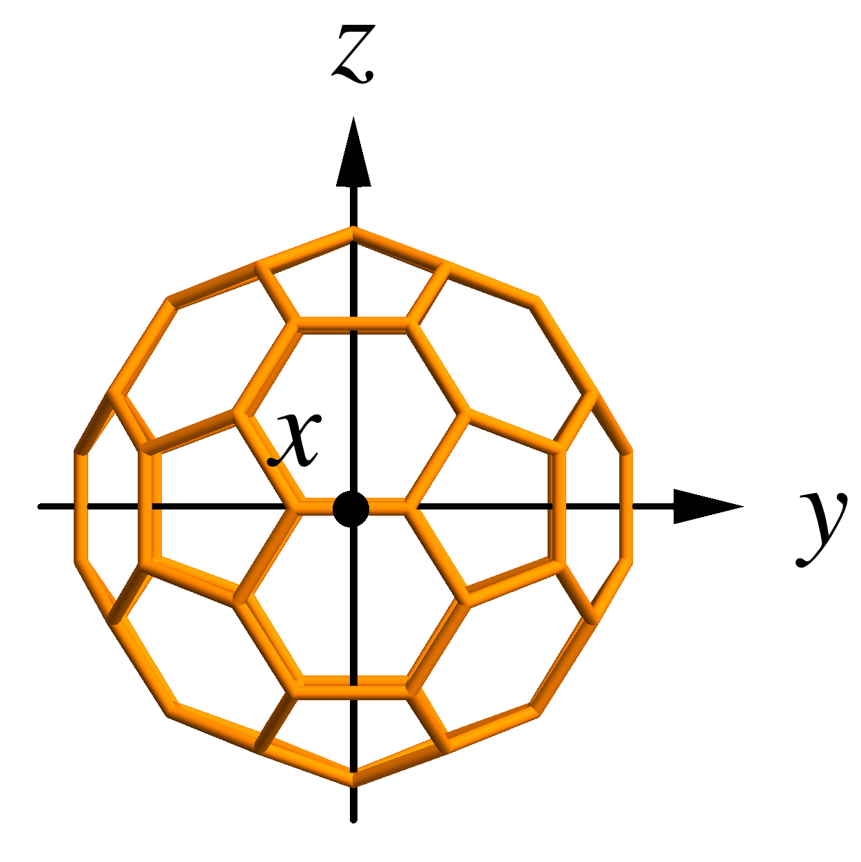
Figure 1: (color online) Orientation of C₆₀ with respect to tetragonal axes of fcc lattice.

The tight-binding Hamiltonian (2) has been parametrized on the basis of density functional theory (DFT) band structure calculation of K₃C₆₀ and includes nearest neighbor and next-nearest-neighbor electron transfer (see Appendix A for details). Although nearest neighbor tight-binding models were intensively used in the past to describe the LUMO bands of fullerides, Gelfand and Lu (1992); Chibotaru and Ceulemans (2000) the inclusion of next-nearest-neighbor electron transfer is necessary for realistic description of the band dispersion. Nomura et al. (2012); Iwahara and Chibotaru (2013) The JT effect in fullerene anions involves eight vibrational $h_{g}$ modes, i.e., 40 vibrational coordinates. Gunnarsson (1997a) The corresponding vibronic coupling parameters for C${}_{60}^{3-}$ have been recently extracted from DFT calculation, Iwahara and Chibotaru (2013) while the reliability of this approach was proven by a satisfactory reproduction of photoemission spectrum for C${}_{60}^{-}$. Iwahara et al. (2010) Nevertheless, in the present calculations the use of a full multimode description of JTE on fullerene sites seems to be impractical. For this reason, the eight-mode JT interaction on fullerenes has been replaced with an effective single-mode one (3). Thus the two parameters, $\hslash\omega=$ 87.7 meV and $g=$ 1.07 were obtained via the reproduction of the JT stabilization energy and the energies of the lowest vibronic excitation of C${}_{60}^{3-}$ ion. Iwahara and Chibotaru (2013) In the model JT Hamiltonian (3), the quadratic vibronic couplings are not included because, as we discussed in Ref. Iwahara and Chibotaru, 2013, they are weak in C₆₀ anions and do not give significant effect on the JT dynamics of C${}_{60}^{n-}$ in cubic fullerides. Finally, the Hund’s rule coupling parameter, $J_{\rm H}=$ 44 meV, was also taken from the DFT calculations. Iwahara and Chibotaru (2013) This is not the case of interelectron repulsion parameters of fullerene site, which are strongly renormalized by screening in fullerides. Gunnarsson (1997a) In the present work, the Coulomb repulsion $U$ is treated as a free parameter. $U$ is defined here as the average repulsion of two electrons in C${}_{60}^{3-}$ for a cubic (undistorted) LUMO band:

$$U=\frac{1}{5}\left(U_{\parallel}+4U_{\perp}\right)=U_{\perp}+\frac{2}{5}J_{\rm H}.$$ (5)

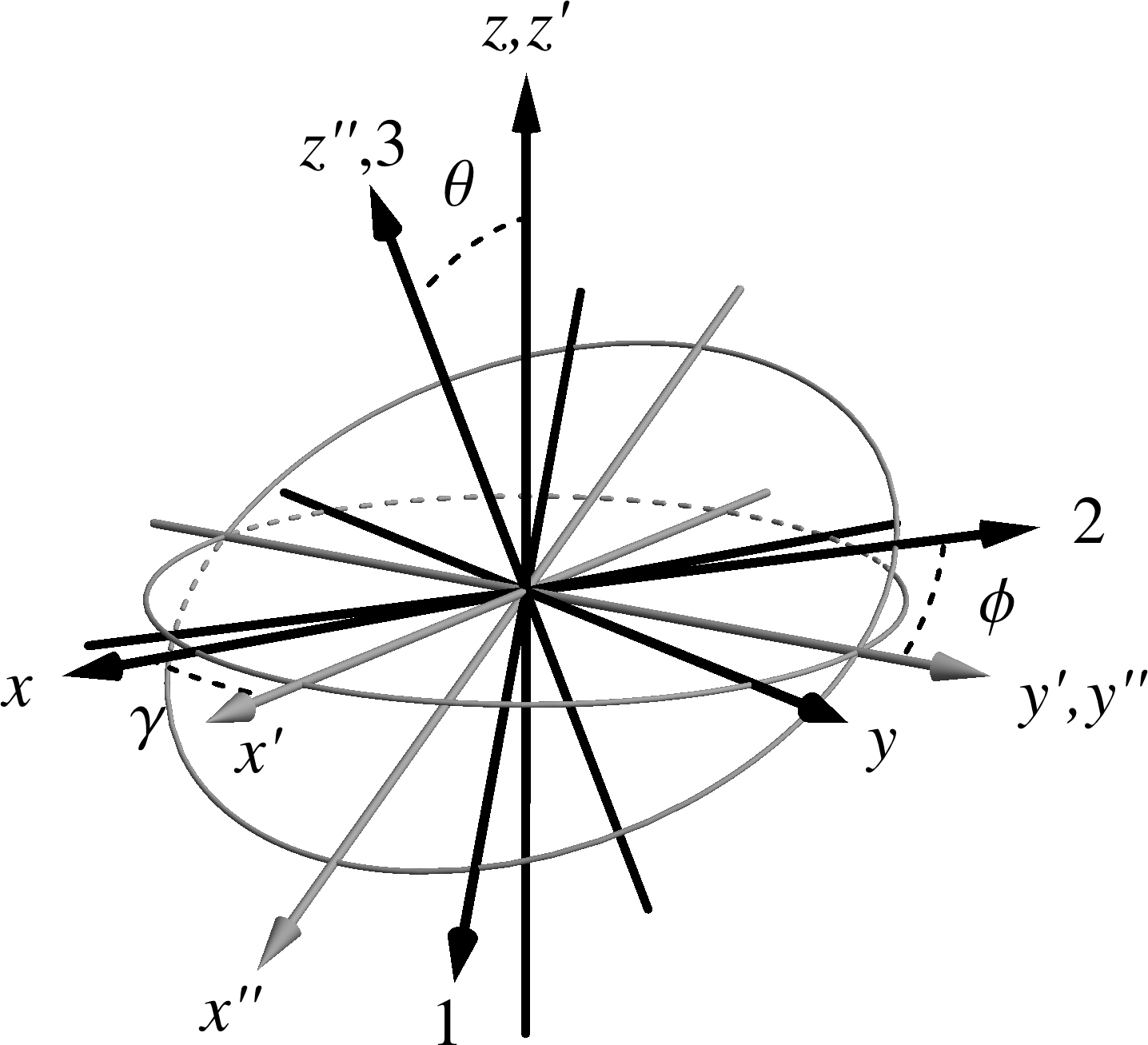
Figure 2: (color online) The coordinate systems used to describe JT effect on a fullerene site. $x,y,z$ correspond to the orthorhombic LUMO orbitals (Fig. 1) and $1,2,3$ to the adiabatic orbitals. $x^{\prime},y^{\prime},z^{\prime}$ and $x^{\prime\prime},y^{\prime\prime},z^{\prime\prime}$ are intermediate coordinate systems Landau and Lifshitz (1977) appearing during the Euler rotation of the orbitals from $x,y,z$ to $1,2,3$, Eq. (6).

II.1 Adiabatic orbitals

The $h_{g}$ normal coordinates on each site $\mathbf{m}$, $q_{\mathbf{m}\gamma}$, are expressed by polar coordinates, $(q_{\mathbf{m}},\alpha_{\mathbf{m}},\gamma_{\mathbf{m}},\theta_{\mathbf{m}},\phi_{\mathbf{m}})$. O’Brien (1996) Introducing a unitary matrix,

$$S_{l\lambda}(\Omega_{\mathbf{m}}) = \left[B_{P}(\gamma_{\mathbf{m}})C_{P}(\theta_{\mathbf{m}})D_{P}(\phi_{\mathbf{m}})\right]_{l\lambda},$$ (6)

we transform the electronic basis $(\lambda=x,y,z)$ into adiabatic basis $(l=1,2,3)$ on each C₆₀ site (Fig. 2),

$$\hat{c}_{\mathbf{m}l\sigma}^{\dagger} = \sum_{\lambda=x,y,z}S_{l\lambda}(\Omega_{\mathbf{m}})\hat{c}_{\mathbf{m}\lambda\sigma}^{\dagger}.$$ (7)

Here, $\Omega_{\mathbf{m}}=(\gamma_{\mathbf{m}},\theta_{\mathbf{m}},\phi_{\mathbf{m}})$, and $B_{P}$, $C_{P}$, $D_{P}$ are the Euler rotational matrices defined in Ref. O’Brien, 1996. By the transformation of the electronic basis, Eq. (7), the linear vibronic term $\hat{U}_{\rm LJT}$ of the JT Hamiltonian (3) becomes diagonal:

$$\hat{\tilde{U}}_{\rm LJT} = \hat{S}^{\dagger}\hat{U}_{\rm LJT}\hat{S}$$ (8)

$$= \sum_{\mathbf{m}}\sum_{\sigma}\hslash\omega gq_{\mathbf{m}}\left[\cos\left(\alpha_{\mathbf{m}}+\frac{\pi}{3}\right)\hat{n}_{\mathbf{m}1\sigma}\right.$$

$$+ \left.\cos\left(\alpha_{\mathbf{m}}-\frac{\pi}{3}\right)\hat{n}_{\mathbf{m}2\sigma}-\cos\alpha_{\mathbf{m}}\hat{n}_{\mathbf{m}3\sigma}\right],$$

where $\hat{S}=\prod_{\mathbf{m}}\hat{S}_{\mathbf{m}}$, and $\hat{S}_{\mathbf{m}}$ is the unitary operator whose matrix element is given by Eq. (6). Eq. (8) shows that the amplitude of the JT distortion is determined by radial coordinates $q_{\mathbf{m}}$ and $\alpha_{\mathbf{m}}$, and the direction of the JT distortion in the space of the five dimensional $h_{g}$ normal coordinates is defined by Euler angular coordinates $\Omega_{\mathbf{m}}$ (Fig. 2). In the described coordinate system, the elastic energy term in Eq. (3) is written as

$$U_{\rm el} = \sum_{\mathbf{m}}\frac{\hslash\omega}{2}q_{\mathbf{m}}^{2},$$ (9)

i.e., is invariant under the unitary transformation (6). On the other hand, the kinetic energy term changes, which is discussed in Sec. IV.2.

Under the transformation of the electronic basis (7), the transfer Hamiltonian (2) becomes

$$\hat{\tilde{H}}_{\rm t}=\hat{S}^{\dagger}\hat{H}_{\rm t}\hat{S}=\sum_{\mathbf{m},\mathbf{m}^{\prime}}\sum_{ll^{\prime}\sigma}t^{\mathbf{m}\mathbf{m}^{\prime}}_{ll^{\prime}}\hat{c}_{\mathbf{m}l\sigma}^{\dagger}\hat{c}_{\mathbf{m}^{\prime}l^{\prime}\sigma},$$ (10)

where $t_{ll^{\prime}}^{\mathbf{m}\mathbf{m}^{\prime}}$ is

$$t^{\mathbf{m}\mathbf{m}^{\prime}}_{ll^{\prime}}(\Omega_{\mathbf{m}},\Omega_{\mathbf{m}^{\prime}}) = \sum_{\lambda\lambda^{\prime}=x,y,z}S_{\lambda l}(\Omega_{\mathbf{m}})t_{\lambda\lambda^{\prime}}^{\mathbf{m}-\mathbf{m}^{\prime}}S_{\lambda^{\prime}l^{\prime}}(\Omega_{\mathbf{m}^{\prime}}).$$

We note also that $\hat{H}_{\rm bi}$ is invariant under the unitary transformation (6) due to the isomorphism of $t_{1u}^{n}$ LUMO shell of C${}_{60}^{n-}$ to the atomic $p^{n}$ shell.

For any Euler angles, $\Omega_{\mathbf{m}}$, the JT potential term, Eqs. (8) and (9), and the bielectronic term has the same form. Therefore, the adiabatic potential energy surface of an isolated C${}_{60}^{n-}$ has continuous minima (trough) Auerbach et al. (1994); O’Brien (1996) even in the presence of the term splitting. In the case of C${}_{60}^{3-}$, the potential surface has three dimensional (3D) trough at

$$q=\sqrt{3}g\sqrt{1-\left(\frac{J_{\rm H}/\hslash\omega}{3g^{2}}\right)^{2}}$$ (12)

and $\alpha=\pi/2$. Substituting $g$, $\omega$, and $J_{\rm H}$ above into Eq. (12), the amplitude of the JT distortion is $q=0.989\times\sqrt{3}g$, indicating that the effect of the Hund’s rule coupling on the JT potential surface of C${}_{60}^{3-}$ is small.

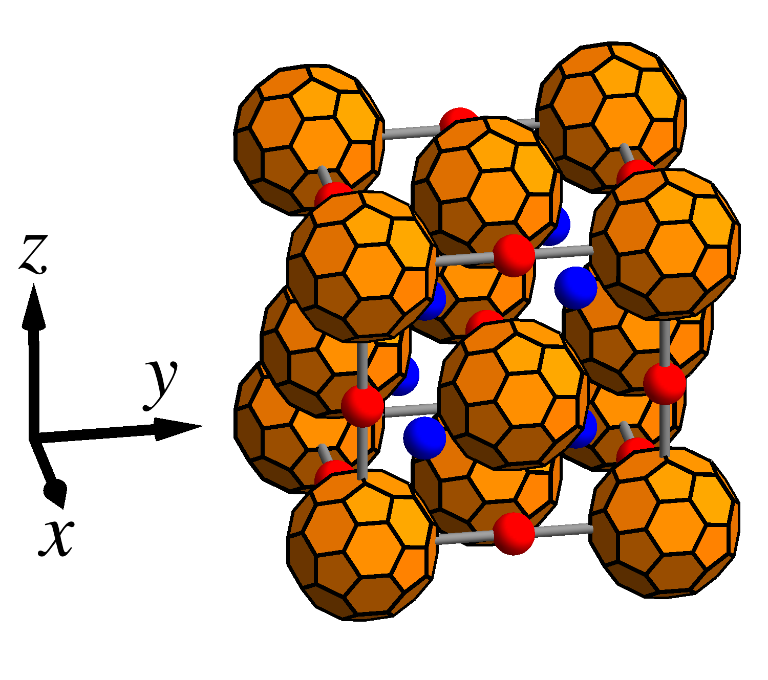
Figure 3: (color online) Ordered fcc K₃C₆₀. The orange ball is C₆₀, and the red and blue spheres are K atoms in octahedral and tetrahedral interstices.

III Gutzwiller approach to Static Jahn-Teller systems

III.1 Self-consistent Gutzwiller approach for the LUMO bands

The merohedral disorder in the K₃C₆₀ lattice and the orientation of the JT distortions on the fullerene sites do not have important effect on the band energy. Ceulemans et al. (1997); Chibotaru and Ceulemans (2000) The change in Hartree-Fock energy per C₆₀ site due to the disorders is only 14 meV, Ceulemans et al. (1997) which is smaller than the JT energy of C${}_{60}^{3-}$ by one order of magnitude. The variation will be further reduced by the electron correlation as is discussed in Sec. IV.2. Therefore, for the sake of simplicity, we further consider a K₃C₆₀ in an ordered fcc lattice (Fig. 3). As a possible scenario of static JT effect we consider equal JT distortions on fullerene sites of the following form:

$$(q_{\mathbf{m}},\alpha_{\mathbf{m}},\gamma_{\mathbf{m}},\theta_{\mathbf{m}},\phi_{\mathbf{m}})=(q,\pi/2,0,0,0),$$ (13)

or in conventional coordinates:

$$(q_{\mathbf{m}\theta},q_{\mathbf{m}\epsilon},q_{\mathbf{m}\xi},q_{\mathbf{m}\eta},q_{\mathbf{m}\zeta})=(0,\sqrt{3}q,0,0,0),$$ (14)

which do not remove translational symmetry of the lattice. Here, $q$ is a variable. The direction of the JT distortion (13) corresponds to the one which gives the maximal static JT stabilization in the case of isolated C${}_{60}^{3-}$ ion. Auerbach et al. (1994); O’Brien (1996) Under the distortion (13), the adiabatic orbitals $l=1,2,3$ correspond to $x,y,z$, respectively (Fig. 2), and the linear JT term (8) reduces to

$$\hat{\tilde{U}}_{\rm LJT} = \sum_{\mathbf{m}}\sum_{\sigma}-\frac{\sqrt{3}}{2}\hslash\omega gq\left(\hat{n}_{\mathbf{m}x\sigma}-\hat{n}_{\mathbf{m}y\sigma}\right).$$ (15)

This expression shows that the $z$ orbital level remains unchanged while the $x$ and the $y$ levels are stabilized and destabilized, respectively. Auerbach et al. (1994); O’Brien (1996)

The Gutzwiller wave function, $|\Psi_{\rm G}\rangle$, is expressed as

$$|\Psi_{\rm G}\rangle = \hat{P}_{\rm G}|\Phi_{\rm S}\rangle,$$ (16)

where $|\Phi_{\rm S}\rangle$ is a Slater determinant, and $\hat{P}_{\rm G}$ is a Gutzwiller projector. The Slater determinant is written as follows:

$$|\Phi_{\rm S}\rangle = \prod_{p\mathbf{k}\sigma}^{\rm occ}\hat{a}_{p\mathbf{k}\sigma}^{\dagger}|0\rangle,$$ (17)

$$\hat{a}_{p\mathbf{k}\sigma}^{\dagger} = \sum_{\mathbf{m}\lambda}\frac{e^{i\mathbf{k}\cdot\mathbf{m}}}{\sqrt{N}}u_{\lambda,p\mathbf{k}}\hat{c}_{\mathbf{m}\lambda\sigma}^{\dagger},$$ (18)

where $p$ is a band index, $N$ is the number of sites in the system, and $u_{\lambda,p\mathbf{k}}$ is a variational orbital coefficient. We note that the band described by $|\Phi_{\rm S}\rangle$ is not constrained to obey the cubic symmetry. In order to include properly the effect of JT distortions and of electron correlation, the variational parameters ($A$) in $\hat{P}_{\rm G}$ have to be orbital-specific:

$$\hat{P}_{\rm G} = \prod_{\mathbf{m}}\exp\left(-\frac{1}{2}\sum_{\lambda\sigma\neq\lambda^{\prime}\sigma^{\prime}}A_{\lambda\lambda^{\prime}}\hat{n}_{\mathbf{m}\lambda\sigma}\hat{n}_{\mathbf{m}\lambda^{\prime}\sigma^{\prime}}\right),$$ (19)

where $A_{\lambda\lambda^{\prime}}$ are real and symmetric with respect to interchange of indices. Therefore, the projector (19) is described by six independent Gutzwiller parameters ($A_{\lambda\lambda^{\prime}}$) instead of a single parameter used in conventional Gutzwiller wave function. Gutzwiller (1963); Vollhardt (1984) In a general case, $\lambda,\lambda^{\prime}$ denote natural orbitals on the site $\mathbf{m}$. For the chosen JT distortions (13), preserving the orthorhombic site-symmetry, these natural orbitals coincide with the orthorhombic $x,y,z$ $t_{1u}$ LUMO orbitals. Due to equal distortions (13) on all fullerene sites, $A_{\lambda\lambda^{\prime}}$ are independent from the index $\mathbf{m}$.

The calculations of expectation values with $|\Psi_{\rm G}\rangle$ have been done within the Gutzwiller’s approximation. Vollhardt (1984); Ogawa et al. (1975) Within this approximation, the energy per site,

$$E_{\rm g} = \frac{1}{N}\frac{\langle\Psi_{\rm G}|\hat{H}|\Psi_{\rm G}\rangle}{\langle\Psi_{\rm G}|\Psi_{\rm G}\rangle},$$ (20)

consists of the band energy,

$$E_{\rm t} = \sum_{\lambda\lambda^{\prime}\sigma}q_{\lambda\lambda^{\prime}}\tau_{\lambda\lambda^{\prime}},$$ (21)

the elastic energy (9), the linear vibronic energy,

$$U_{\rm LJT} = \sum_{\sigma}-\frac{\sqrt{3}}{2}\hslash\omega gq\left(n_{x}-n_{y}\right),$$ (22)

and the bielectronic energy $E_{\rm bi}$. Here, $q_{\lambda\lambda^{\prime}}$ is the Gutzwiller’s reduction factor, $\tau_{\lambda\lambda^{\prime}}$ is

$$\tau_{\lambda\lambda^{\prime}} = \frac{1}{N}\sum_{\mathbf{k}}t_{\lambda\lambda^{\prime}}^{\mathbf{k}}\rho_{\lambda\lambda^{\prime}}^{\mathbf{k}},$$ (23)

where $t_{\lambda\lambda^{\prime}}^{\mathbf{k}}$ is the Fourier transform of $t_{\lambda\lambda^{\prime}}^{\Delta\mathbf{m}}$,

$$t_{\lambda\lambda^{\prime}}^{\mathbf{k}} = \sum_{\Delta\mathbf{m}}e^{-i\mathbf{k}\cdot\Delta\mathbf{m}}t_{\lambda\lambda^{\prime}}^{\Delta\mathbf{m}},$$ (24)

$\rho_{\lambda\lambda^{\prime}}^{\mathbf{k}}$ is the density matrix at a $\mathbf{k}$ point,

$$\rho_{\lambda\lambda^{\prime}}^{\mathbf{k}} = \sum_{p}^{\rm occ}u_{\lambda,p\mathbf{k}}^{*}u_{\lambda^{\prime},p\mathbf{k}},$$ (25)

and $n_{\lambda}$ $(\lambda=x,y,z)$ is the occupation number,

$$n_{\lambda} = \frac{\langle\Psi_{\rm G}|\hat{n}_{\mathbf{m}\lambda\sigma}|\Psi_{\rm G}\rangle}{\langle\Psi_{\rm G}|\Psi_{\rm G}\rangle}.$$ (26)

The explicit forms of the occupation number $n_{\lambda}$, the Gutzwiller’s reduction factor $q_{\lambda\lambda^{\prime}}$, and the bielectronic energy $E_{\rm bi}$ are given in Appendix B. The Gutzwiller projector does not influence the on-site density matrix, hence, Eq. (26) corresponds to

$$n_{\lambda} = \langle\Phi_{\rm S}|\hat{n}_{\mathbf{m}\lambda\sigma}|\Phi_{\rm S}\rangle=\frac{1}{N}\sum_{\mathbf{k}}\rho_{\lambda\lambda}^{\mathbf{k}}.$$ (27)

Hereafter, we use the form (27) for $n_{\lambda}$.

The ground state for different amplitudes of JT distortion $q$ is obtained by minimizing the energy per site (20) with respect to $\{u_{\lambda,p\mathbf{k}}\}$ and $\{A_{\lambda\lambda^{\prime}}\}$, which is performed in two steps. The first one is the variational calculation of $\tilde{E}_{\rm g}$ with respect to $\{u_{\lambda,p\mathbf{k}}\}$ for fixed $\{A_{\lambda\lambda^{\prime}}\}$. The resulting self-consistent equations in the case of static JT effect are obtained in the form:

$$\sum_{\lambda^{\prime}}h_{\lambda\lambda^{\prime}}^{\mathbf{k}}u_{\lambda^{\prime},p\mathbf{k}}=\epsilon_{p\mathbf{k}}u_{\lambda,p\mathbf{k}},$$ (28)

where the one-particle Hamiltonian is

$$h_{\lambda\lambda^{\prime}}^{\mathbf{k}} = q_{\lambda\lambda^{\prime}}t_{\lambda\lambda^{\prime}}^{\mathbf{k}}+\delta_{\lambda\lambda^{\prime}}\left[\sum_{\kappa\kappa^{\prime}}\frac{\partial q_{\kappa\kappa^{\prime}}}{\partial n_{\lambda}}\tau_{\kappa\kappa^{\prime}}+\frac{1}{2}\frac{\partial E_{\rm bi}}{\partial{n}_{\lambda}}\right.$$ (29)

$$- \left.\frac{\sqrt{3}}{2}\hslash\omega gq\left(\delta_{\lambda x}-\delta_{\lambda y}\right)\right],$$

and $\epsilon_{p\mathbf{k}}$ is the Gutzwiller’s orbital energy. Using the solutions of Eq. (28), $\{u_{\lambda,p\mathbf{k}}\}$, the occupation numbers $\{n_{\lambda}\}$ are recalculated via Eq. (27). The chemical potential is found by consecutive population of Gutzwiller’s orbitals following the aufbau principle. The second step is the minimization of $\tilde{E}_{\rm g}$ with respect to $\{A_{\lambda\lambda^{\prime}}\}$ for fixed $\{u_{\lambda,p\mathbf{k}}\}$ and $\{n_{\lambda}\}$,

$$\frac{\partial\tilde{E}_{\rm g}}{\partial A_{\lambda\lambda^{\prime}}} = \sum_{\sigma\kappa\kappa^{\prime}}\frac{\partial q_{\kappa\kappa^{\prime}}}{\partial A_{\lambda\lambda^{\prime}}}\tau_{\kappa\kappa^{\prime}}+\frac{\partial E_{\rm bi}}{\partial A_{\lambda\lambda^{\prime}}}=0,$$ (30)

using the numerical algorithm proposed in Ref. Bünemann et al., 2012. The two minimizations, (28) and (30), are repeated iteratively until variations in the occupation numbers and the ground state energy become smaller than thresholds.

(a)

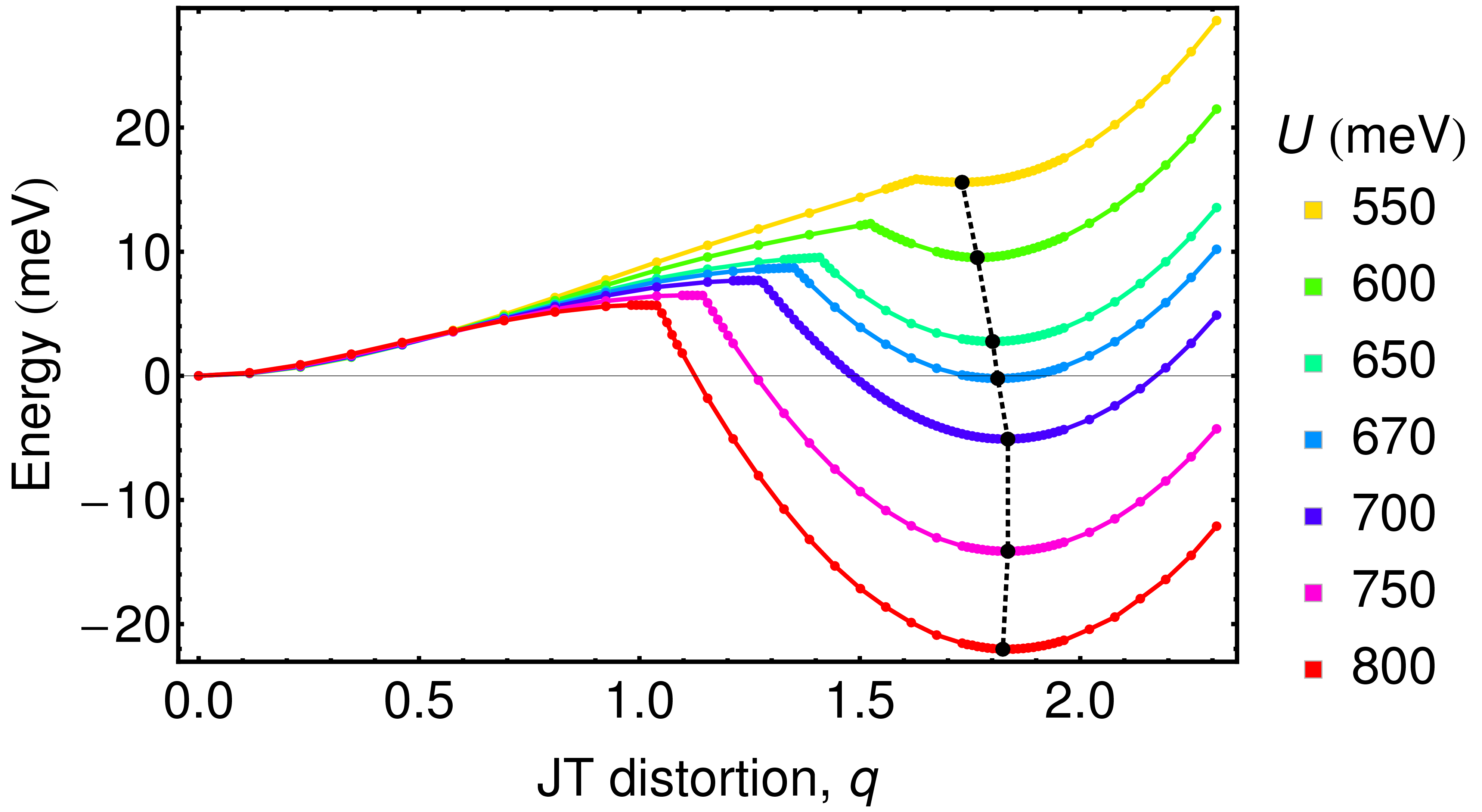
(b)

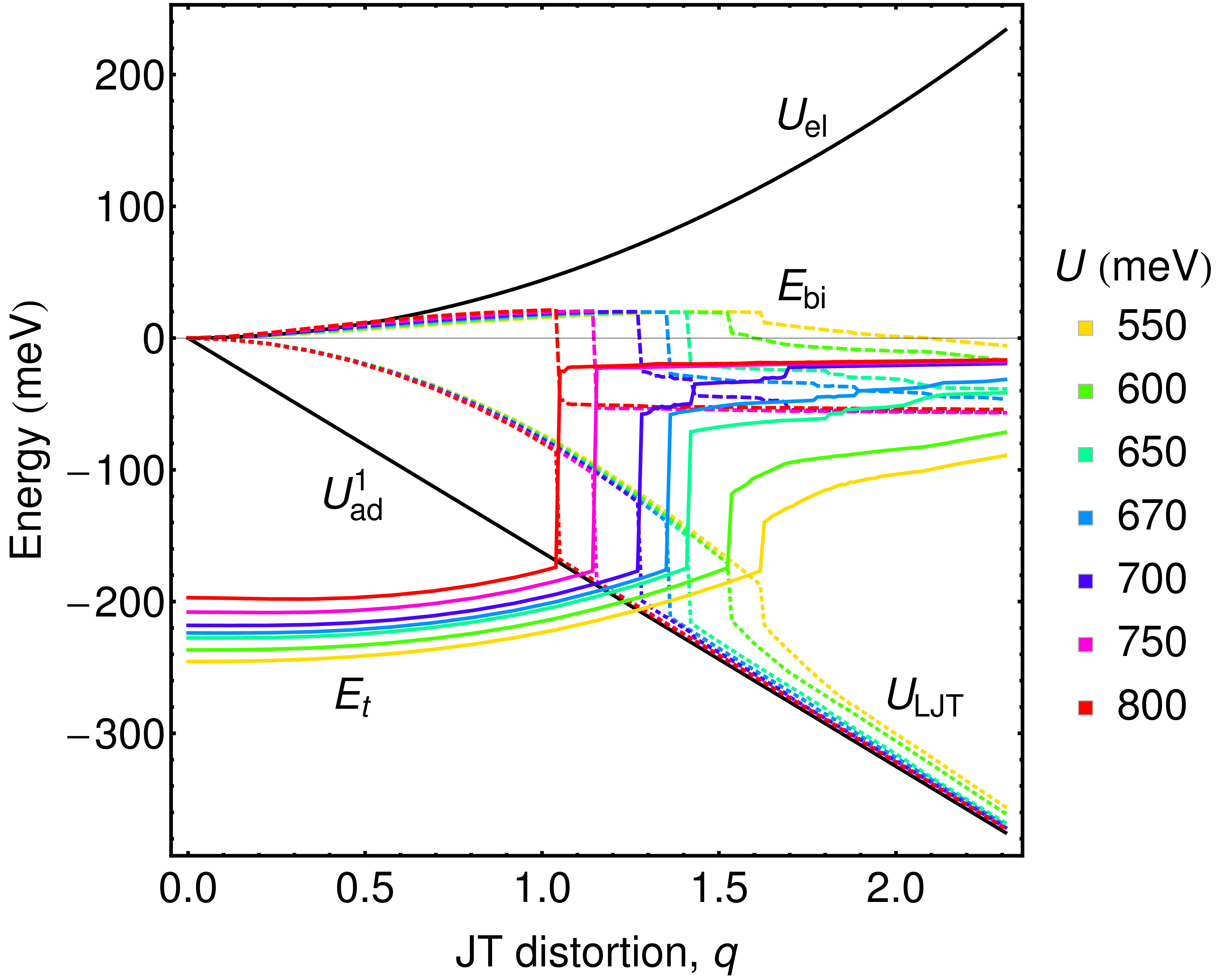
(c)

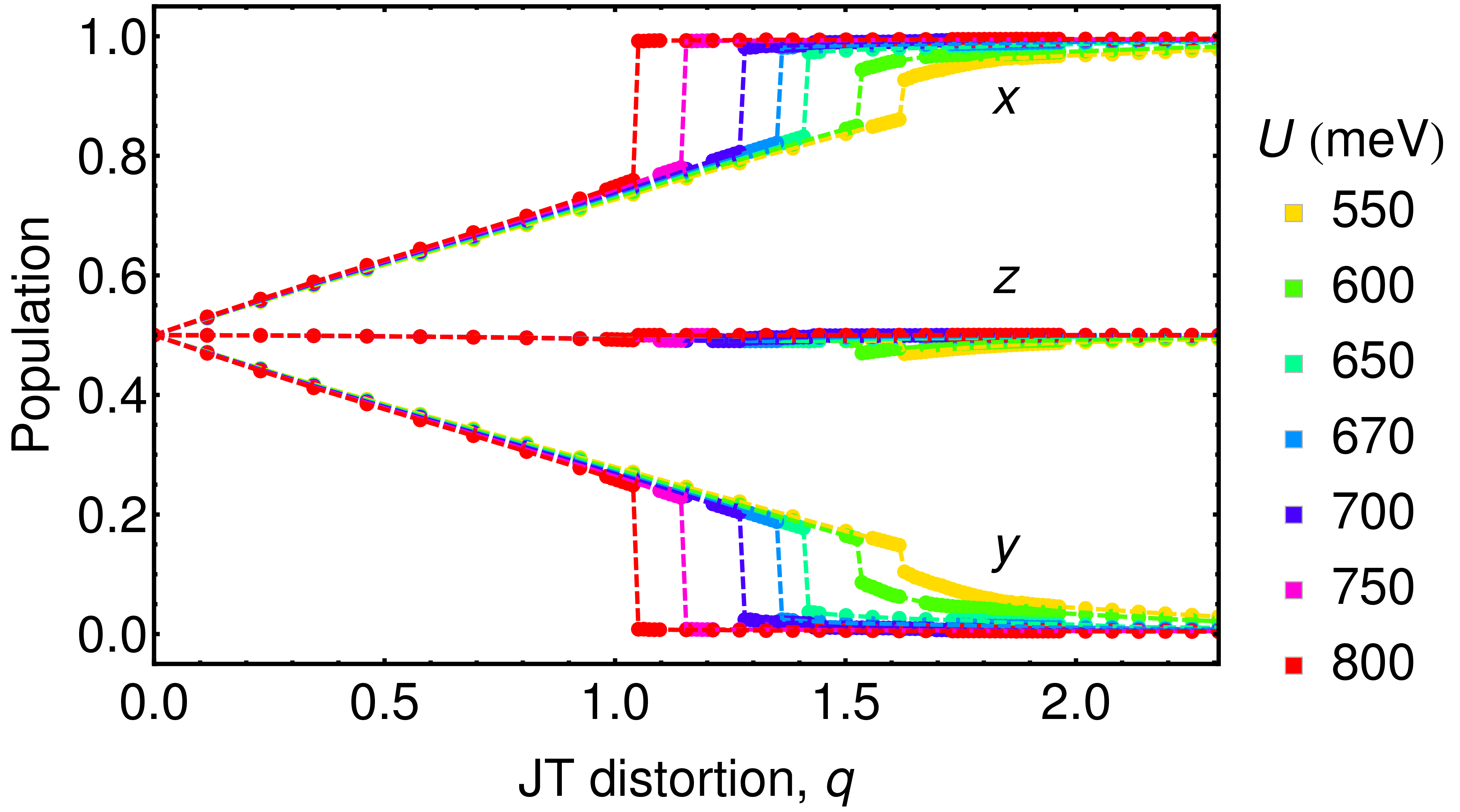
Figure 4: (color online) (a) Total energy $E_{\rm g}(q)$ of K₃C₆₀ as function of amplitude of static JT distortion (13) for several values of $U$ (5). The dashed line indicates the minimum of $E_{\rm g}$. (b) Energy components contributing to the total energy. $U_{\rm LJT}$ is the linear JT energy (8) and $U_{\rm el}$ is the elastic energy (9) in $\hat{H}_{\rm JT}$; $E_{\rm t}$ is the band energy (21), and $E_{\rm bi}$ is the bielectronic energy. $U_{\rm ad}^{1}$ is the ground state adiabatic potential of an isolated C${}_{60}^{3-}$. $E_{\rm g}$ and $E_{\rm bi}$ are set to zero at $q$=0. The unit of $q$ is the amplitude of zero-vibration of $h_{g}$ mode. Bersuker and Polinger (1989); Bersuker (2006) (c) Occupation numbers of LUMO orbitals $n_{\lambda}$ as function of $q$. $x$, $y$, and $z$ are orbital components.

III.2 Static Jahn-Teller instability in K₃C₆₀

The ground state energy $E_{\rm g}$ (20) as a function of the JT distortion $q$ is plotted in Fig. 4a. Quite unexpectedly, the energy curve $E_{\rm g}(q)$ has two minima, one at the undistorted configuration $q=0$ and the other at $q\approx\sqrt{3}g$ $(=1.85)$ which corresponds approximately to the amplitude of JT distortion in an isolated C${}_{60}^{3-}$ ion. For $U$ smaller than the critical value $U_{c}=$ 670 meV the static JT distortion is quenched ($q=0$). The minimum corresponding to JT-distorted sites lowers with the increase of $U$, at $U=U_{c}$ the values of the two minima equalize and for $U>U_{c}$ the JT distortion achieves its equilibrium value matching approximately the distortion in an isolated C${}_{60}^{3-}$.

The static JT effect has been investigated in $A_{4}$C₆₀ within the local density approximation (LDA) of DFT, for which completely quenched JT distortions have been found. Capone et al. (2000) Since the static JT effect in C${}_{60}^{4-}$ is stronger than in C${}_{60}^{3-}$ anion, Auerbach et al. (1994) it was concluded that the JT distortions in $A_{3}$C₆₀ are also quenched. However it was recently revealed that the LDA calculations underestimate the JT stabilization energy of C${}_{60}^{-}$ by ca 30 %. Iwahara et al. (2010) On the other hand the broken-symmetry Hartree-Fock (HF) calculations predict smaller $U_{c}$ for static JT instability than the present calculations and orbital disproportionation of the intrasite charge density in fullerides. Chibotaru and Ceulemans (1996); Ceulemans et al. (1997) The reason of this discrepancy is that the broken-symmetry HF calculations exaggerate the tendency towards the stabilization of low-symmetry electronic phases. Thus the splitting of the LUMO band is overestimated and is mainly contributed by the interelectron repulsion, Ceulemans et al. (1997) suggesting that an approach based on a single Slater determinant is not flexible enough to include properly the effects of electron correlation in orbitally degenerate bands (see Sec. V.1 for detailed discussion).

The structure of $E_{\rm g}(q)$ is mainly determined by the $q$-dependent contributions, the band energy $E_{\rm t}$ (21) and the JT potential $U_{\rm LJT}$ (22) which are found in competition (Fig. 4b). The contribution of the band energy term is the largest when the orbitals are hybridized and equally populated, which takes place in the weak correlation limit ($U\rightarrow 0$). On the other hand, the contribution from the JT term is the largest when the disproportionation of the electronic charge among the LUMO subbands, accompanying the JT distortions, is full, $(n_{x},n_{y},n_{z})=(1,0,1/2)$. At the same time, the splitting of the orbital levels prevents the hybridization and vice versa. As Fig. 4a suggests, the ground state energy $E_{\rm g}(q)$ consists of two potential energy surfaces which cross at $q=q_{c}$. For small distortions $q<q_{c}$, the band energy exceeds the JT energy and the latter is quenched compared to the case of an isolated C${}_{60}^{3-}$ ($U_{\rm ad}^{1}$), while for $q>q_{c}$ the JT energy takes over. Because of the hybridization, the occupation numbers $n_{\lambda}$ are fractional (Fig. 4c) and the linear JT energy $U_{\rm LJT}$ is not proportional to $q$ unlike the isolated C${}_{60}^{3-}$ molecule. The band energy is reduced by the intrasite Coulomb repulsion by quenching charge fluctuations on C₆₀’s. Since the band energy in Rb₃C₆₀ and Cs₃C₆₀ is smaller than in K₃C₆₀, while $U$ is larger, Nomura et al. (2012) the static JT instability is favored even more in these fullerides.

IV Gutzwiller approach to dynamical Jahn-Teller systems

IV.1 Dynamical Jahn-Teller contribution

Another important ingredient is the energy gain arising from the dynamical delocalization of JT distortions at each C${}_{60}^{3-}$ anion. The energy gain in isolated C${}_{60}^{3-}$ amounts to ca 90 meV which is more than a half of the static JT stabilization (ca 150 meV) in this anion. Iwahara and Chibotaru (2013) To assess this energy gain in fullerides, one should take into account that the JT effect on C${}_{60}^{3-}$ sites in fullerides is different from the case of isolated fullerene anions. The main difference is that the LUMO orbitals on the fullerene sites do not have the same populations as in an isolated C${}_{60}^{3-}$ (Fig. 4c), which leads, in particular, to lower values of the amplitude of dynamical JT deformation in fullerides. Only in the case of full orbital disproportionation (Sec. III.2) the deformation achieves the equilibrium value in a free ion ($q=1.85$) and the corresponding energy gain owing to dynamical JT effect is maximal. One should stress that in the case of dynamic JT effect the adiabatic orbitals $l=1,2,3$ on fullerene sites are not fixed electronic orbitals $\lambda=x,y,z$, considered in the previous section but are their linear combinations with $\Omega_{\mathbf{m}}$-dependent coefficients, Eq. (7). O’Brien (1996) To simulate the dependence of dynamical JT effect on the extent of orbital disproportionation, we introduce the effective vibronic coupling constant,

$$g_{\rm eff}=g(n_{1}-n_{2}),$$ (31)

which varies from 0 to $g$ when the orbital disproportionation $n_{1}-n_{2}$ varies from the minimal value (0) to the maximal value (1). Note that $n_{3}$ has an unchanged value $1/2$.

Diagonalizing the JT Hamiltonian (3) for different values of $g_{\rm eff}$, and extracting the ground state energy at corresponding static JT distortion, $3\hslash\omega g_{\rm eff}^{2}/2$, together with the energy of zero-vibrations at distorted point, $5\hslash\omega/2$, we obtain the dynamical contribution, $E_{\rm DJT}$, to the ground vibronic level. Figure 5 shows the dependence of this contribution on $g_{\rm eff}$ for the case of effective single-mode JT Hamiltonian of C${}_{60}^{3-}$. Iwahara and Chibotaru (2013) Note that the existence of the energy gain due to dynamical delocalization of JT deformations does not guarantee by itself the development of dynamical JT effect on fullerene sites. For the latter to take place, an additional condition are the small variations of the band energy under arbitrary JT distortion on C${}_{60}^{3-}$ sites, which is investigated below.

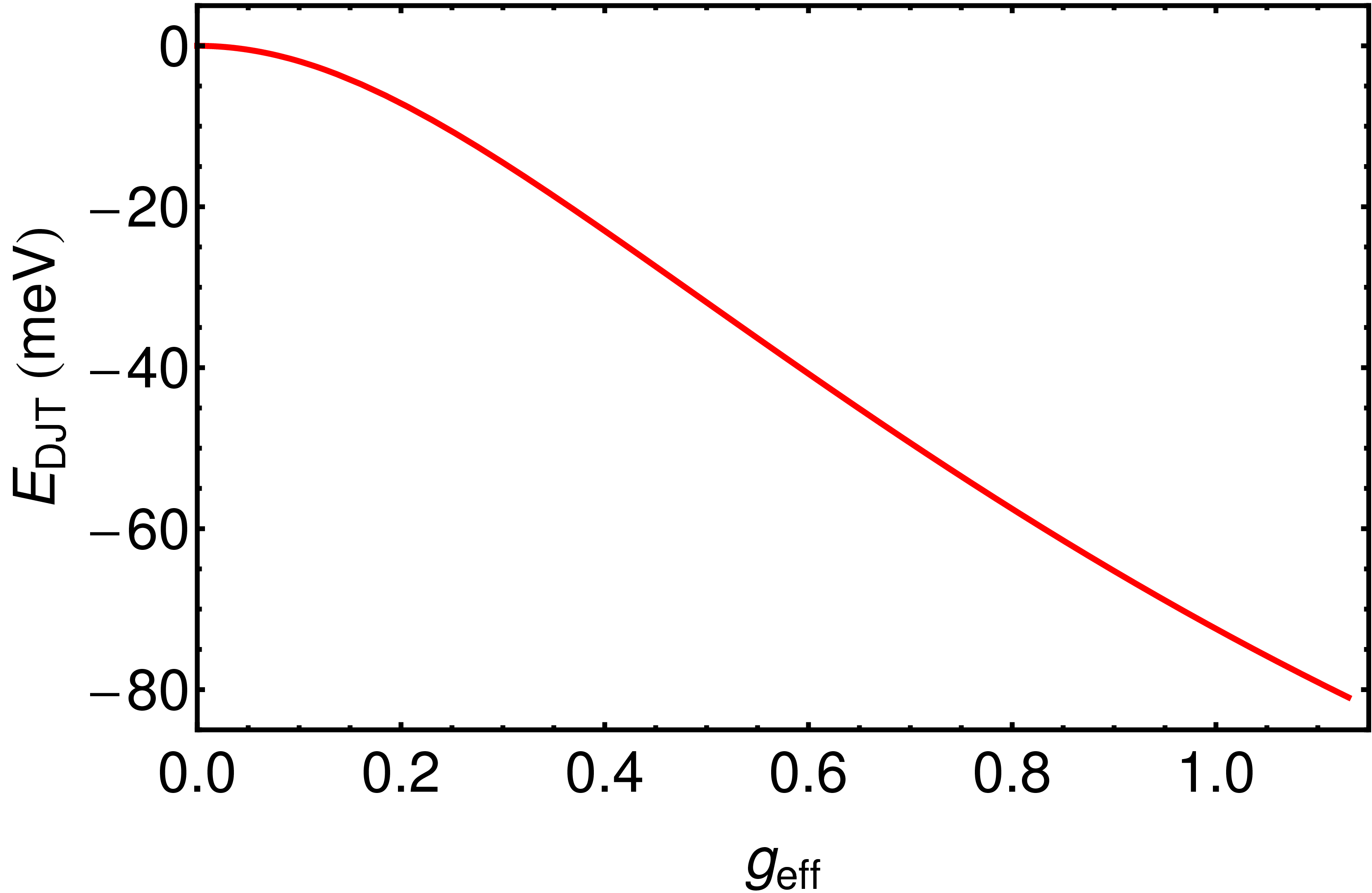
Figure 5: (color online) The gain of JT stabilization energy (meV) due to dynamical JTE in function of $g_{\rm eff}$.

IV.2 Form of the ground vibronic state

Previous ab initio investigations have shown that the low-lying vibronic states in an isolated C${}_{60}^{3-}$ can be described satisfactorily within the adiabatic approximation. Iwahara and Chibotaru (2013) This approximation can be extended over the $A_{3}$C₆₀ crystal. Following the molecular approach, Bersuker and Polinger (1989) first we perform the unitary transformation (7) to diagonalize the linear vibronic term in Eq. (3) Auerbach et al. (1994); O’Brien (1996):

$$\hat{\tilde{H}} = \hat{S}^{\dagger}\hat{H}\hat{S}=\hat{H}_{\rm rad}+\hat{H}_{\rm rot}+\hat{H}^{(1)}_{\rm el}+\hat{H}_{\rm bi},$$ (32)

$$\hat{H}_{\rm rad} = \sum_{\mathbf{m}}-\frac{\hslash\omega}{2}\left[q_{\mathbf{m}}^{-4}\frac{\partial}{\partial q_{\mathbf{m}}}\left(q_{\mathbf{m}}^{4}\frac{\partial}{\partial q_{\mathbf{m}}}\right)\right.$$

$$+ \left.\frac{1}{q_{\mathbf{m}}^{2}\sin 3\alpha_{\mathbf{m}}}\frac{\partial}{\partial\alpha_{\mathbf{m}}}\left(\sin 3\alpha_{\mathbf{m}}\frac{\partial}{\partial\alpha_{\mathbf{m}}}\right)\right]+\frac{\hslash\omega}{2}q_{\mathbf{m}}^{2},$$

$$\hat{H}_{\rm rot} = \sum_{\mathbf{m}}\frac{\hslash\omega}{8q_{\mathbf{m}}^{2}}\left[\frac{(\hat{L}^{\rm nuc}_{\mathbf{m}1}+\hat{L}^{\rm el}_{\mathbf{m}1})^{2}}{\sin^{2}(\alpha_{\mathbf{m}}-2\pi/3)}+\frac{(\hat{L}^{\rm nuc}_{\mathbf{m}2}+\hat{L}^{\rm el}_{\mathbf{m}2})^{2}}{\sin^{2}(\alpha_{\mathbf{m}}+2\pi/3)}\right.$$ (33)

$$+ \left.\frac{(\hat{L}^{\rm nuc}_{\mathbf{m}3}+\hat{L}^{\rm el}_{\mathbf{m}3})^{2}}{\sin^{2}\alpha_{\mathbf{m}}}\right].$$

Here, $\hat{H}^{(1)}_{\rm el}$ is the sum of the linear vibronic term (8) and the transfer part (10), $\hat{L}^{\rm nuc}_{\mathbf{m}1}$, $\hat{L}^{\rm nuc}_{\mathbf{m}2}$, $\hat{L}^{\rm nuc}_{\mathbf{m}3}$ are nuclear angular momenta in the initial orbital basis ($\lambda_{x},\lambda_{y},\lambda_{z}$ in Ref. O’Brien, 1996, respectively), and $\hat{L}^{\rm el}_{\mathbf{m}j}(j=1,2,3)$ are electronic angular momenta:

$$\hat{L}^{\rm el}_{\mathbf{m}1} = \sum_{\sigma}i\left(\hat{c}_{\mathbf{m}2\sigma}^{\dagger}\hat{c}_{\mathbf{m}3\sigma}-\hat{c}_{\mathbf{m}3\sigma}^{\dagger}\hat{c}_{\mathbf{m}2\sigma}\right),$$ (34)

$$\hat{L}^{\rm el}_{\mathbf{m}2} = \sum_{\sigma}i\left(\hat{c}_{\mathbf{m}3\sigma}^{\dagger}\hat{c}_{\mathbf{m}1\sigma}-\hat{c}_{\mathbf{m}1\sigma}^{\dagger}\hat{c}_{\mathbf{m}3\sigma}\right),$$ (35)

$$\hat{L}^{\rm el}_{\mathbf{m}3} = \sum_{\sigma}i\left(\hat{c}_{\mathbf{m}1\sigma}^{\dagger}\hat{c}_{\mathbf{m}2\sigma}-\hat{c}_{\mathbf{m}2\sigma}^{\dagger}\hat{c}_{\mathbf{m}1\sigma}\right).$$ (36)

For arbitrary JT deformations on sites, the system does not possess translational symmetry anymore. In the case of intermediate to strong vibronic coupling, the amplitude of dynamical JT deformation $q_{0}$ is not small. Since the LUMO orbitals of each fullerene are, on average, occupied by three electrons, the vibronic term has a minimum at $\alpha=\pi/2$. O’Brien (1996) Substituting

$$q_{\mathbf{m}}=q_{0}+q^{\prime}_{\mathbf{m}},\qquad\alpha_{\mathbf{m}}=\frac{\pi}{2}+\alpha^{\prime}_{\mathbf{m}},$$ (37)

into Eq. (32), we obtain

$$\hat{\tilde{H}} = \hat{H}_{\rm rad}+\hat{H}_{\rm rot}+\hat{H}_{\rm el}^{(1)}+\hat{H}_{\rm bi},$$ (38)

$$\hat{H}_{\rm rad} = \sum_{\mathbf{m}}-\frac{\hslash\omega}{2}\left[q_{0}^{-4}\frac{\partial}{\partial q^{\prime}_{\mathbf{m}}}\left(q_{\mathbf{m}}^{4}\frac{\partial}{\partial q^{\prime}_{\mathbf{m}}}\right)+\frac{1}{q_{0}^{2}}\frac{\partial^{2}}{\partial\alpha^{\prime 2}_{\mathbf{m}}}\right]_{q_{\mathbf{m}}=q_{0}}$$ (39)

$$+ N\frac{\hslash\omega}{2}q_{0}^{2}+\sum_{\mathbf{m}}\frac{\hslash\omega}{2}{q^{\prime 2}_{\mathbf{m}}},$$

$$\hat{H}_{\rm rot} = \sum_{\mathbf{m}}\frac{\hslash\omega}{8q_{0}^{2}}\left[4\left(\hat{L}^{\rm nuc}_{\mathbf{m}1}+\hat{L}^{\rm el}_{\mathbf{m}1}\right)^{2}+4\left(\hat{L}^{\rm nuc}_{\mathbf{m}2}+\hat{L}^{\rm el}_{\mathbf{m}2}\right)^{2}\right.$$ (40)

$$+ \left.\left(\hat{L}^{\rm nuc}_{\mathbf{m}3}+\hat{L}^{\rm el}_{\mathbf{m}3}\right)^{2}\right],$$

$$\hat{H}_{\rm el}^{(1)} = \sum_{\mathbf{m}}\sum_{\sigma}-\frac{\sqrt{3}}{2}\hslash\omega gq_{0}\left(\hat{n}_{\mathbf{m}1\sigma}-\hat{n}_{\mathbf{m}2\sigma}\right)$$ (41)

$$+ \sum_{\mathbf{m},\mathbf{m}^{\prime}}\sum_{ll^{\prime}\sigma}t^{\mathbf{m}\mathbf{m}^{\prime}}_{ll^{\prime}}\hat{c}_{\mathbf{m}l\sigma}^{\dagger}\hat{c}_{\mathbf{m}^{\prime}l^{\prime}\sigma},$$

where $q^{\prime}_{\mathbf{m}}$ and $\alpha^{\prime}_{\mathbf{m}}$ are the deviations from the equilibrium point. The above derivation is based on the assumption that the radial JT coordinates (37) remain unchanged under the electron transfer. The justification for that, i.e., for the neglect of JT polaronic effect will be given in Sec. VI.3. Following the adiabatic approximation, Bersuker and Polinger (1989) in Eq. (38) the terms smaller than $1/q_{0}^{2}$ are neglected and, consequently, the radial degrees of freedom ($q^{\prime},\alpha^{\prime}$) are decoupled from the other degrees of freedoms corresponding to the rotation of JT deformation in the 3D trough Auerbach et al. (1994); O’Brien (1996) (see Sec. II.1 for the trough). The rotational Hamiltonian (40) has nonadiabatic terms, $\hat{V}=\hslash\omega\hat{L}^{\rm nuc}_{\mathbf{m}j}\hat{L}^{\rm el}_{\mathbf{m}j}/q_{0}^{2}$. Neglecting these terms, Bersuker and Polinger (1989) we obtain

$$\hat{H}_{\rm ad} = \hat{H}_{\rm rad}+\hat{H}_{\rm rot}^{\rm nuc}+\hat{H}_{\rm rot}^{\rm el}+\hat{H}_{\rm el}^{(1)}+\hat{H}_{\rm bi},$$ (42)

$$\hat{H}_{\rm rot}^{\rm nuc} = \sum_{\mathbf{m}}\frac{\hslash^{2}}{8q_{0}^{2}}\left[4\left(\hat{L}^{\rm nuc}_{\mathbf{m}}\right)^{2}-3\left(\hat{L}^{\rm nuc}_{\mathbf{m}3}\right)^{2}\right],$$ (43)

$$\hat{H}_{\rm rot}^{\rm el} = \sum_{\mathbf{m}}\frac{\hslash^{2}}{8q_{0}^{2}}\left[4\left(\hat{L}_{\mathbf{m}}^{\rm el}\right)^{2}-3\left(\hat{L}_{\mathbf{m}3}^{\rm el}\right)^{2}\right],$$ (44)

where $\hat{L}_{\mathbf{m}}^{2}=\hat{L}_{\mathbf{m}1}^{2}+\hat{L}_{\mathbf{m}2}^{2}+\hat{L}_{\mathbf{m}3}^{2}$. The adiabatic approximation is valid when the energy gap between the ground and the first excited energies $\Delta E$ is large compared with the matrix element of the nonadiabatic term $|\hat{V}|$. The ratio of $|\hat{V}|\approx\hslash\omega/(3g^{2})$ and $\Delta E\approx 3\hslash\omega g^{2}/2$ for C${}_{60}^{3-}$ is $|\hat{V}|/\Delta E\approx 1/5$, which justifies the application of adiabatic approximation in the present case. In this estimation, a value $|\hat{L}|\approx 1$ was taken.

Diagonalizing $\hat{H}_{\rm el}^{(1)}$ (41), the Hamiltonian is written in the basis of adiabatic band orbitals:

$$\hat{H}_{\rm el}^{(1)} = \sum_{i\sigma}\epsilon_{i}(\Omega)\hat{a}_{i\sigma}^{\dagger}(\Omega)\hat{a}_{i\sigma}(\Omega),$$ (45)

where $\Omega=\{\Omega_{\mathbf{m}}\}$ is the set of all Euler angles on all C₆₀ sites in the system (Fig. 2), $i$ indicates adiabatic band orbital, $\epsilon_{i}$ denotes its energy, and $\hat{a}_{i\sigma}^{\dagger}$ is given by

$$\hat{a}_{i\sigma}^{\dagger}(\Omega) = \sum_{\mathbf{m}}\sum_{l}U_{\mathbf{m}li}(\Omega)\hat{c}_{\mathbf{m}l\sigma}^{\dagger}.$$ (46)

For the ordered system (13), the coefficient $U_{\mathbf{m}li}$ reduces to $e^{i\mathbf{k}\cdot\mathbf{m}}u_{\lambda,p\mathbf{k}}/\sqrt{N}$ appearing in Eq. (18).

Then the solution of the Hamiltonian (42) in the adiabatic approximation for the ground and low-lying vibronic states has the form:

$$|\Psi(R,\Omega)\rangle = |\Phi_{\rm S}^{\rm ad}(\Omega)\rangle\chi^{\rm rad}(R)\chi^{\rm rot}(\Omega),$$ (47)

where $|\Phi_{\rm S}^{\rm ad}\rangle$ is the Slater determinant of occupied adiabatic band orbitals (46):

$$|\Phi_{\rm S}^{\rm ad}(\Omega)\rangle=\prod_{i\sigma}^{\rm occ}\hat{a}_{i\sigma}^{\dagger}(\Omega)|0\rangle,$$ (48)

and $\chi^{\rm rad}(R)$ and $\chi^{\rm rot}(\Omega)$ are nuclear wave functions depending on radial $R=\{q^{\prime}_{\mathbf{m}},\alpha^{\prime}_{\mathbf{m}}\}$ and rotational $\Omega$ nuclear coordinates, respectively. The factorization of nuclear wave function became possible due to the separation of radial and rotational degrees of freedom in the adiabatic Hamiltonian (42). Furthermore, the radial coordinates of different sites are independent from each other (see Eq. (39)), hence, the radial part $\chi^{\rm rad}$ is the product of the ground vibrational wave functions of all sites:

$$\chi^{\rm rad}(R)=\prod_{\mathbf{m}}\chi^{\rm rad}_{\mathbf{m}}(q^{\prime}_{\mathbf{m}},\alpha^{\prime}_{\mathbf{m}}).$$ (49)

Further calculations are greatly simplified under the assumption that the dependence of $U_{\mathbf{m}li}$ (46) on Euler angles is relatively weak. This seems to be the case when correlation effects become important, leading to significant reduction of band energy $E_{\rm t}$ (Fig. 4b) and strong separation of Gutzwiller bands ($x,y,z$ in Fig. 4c for homogeneous JT distortions (13)). Indeed, the hybridization of the adiabatic orbitals in this case mainly arises via resonant interactions (Fig. 6) because the width of individual bands is small compared with their Jahn-Teller splitting (150 meV), thus resulting in a weak mixing of the off-resonant adiabatic orbitals. The hybridization arising from resonant interactions should be weakly dependent on transfer parameters. For example, in the case of two-site model (Fig. 6), the “band” splitting of pairs of interacting resonant adiabatic orbitals $\Delta\epsilon$ is strongly dependent on the Euler angles on two sites,

$$\Delta\epsilon\approx\left|2t^{AB}_{ll}(\Omega_{A},\Omega_{B})\right|,$$ (50)

while the adiabatic “band” orbitals,

$$|\psi_{i\sigma}(\Omega)\rangle\approx\frac{1}{\sqrt{2}}\left(\hat{c}^{\dagger}_{Al\sigma}\pm\hat{c}^{\dagger}_{Bl\sigma}\right)|0\rangle,$$ (51)

have angle-independent mixing coefficients.

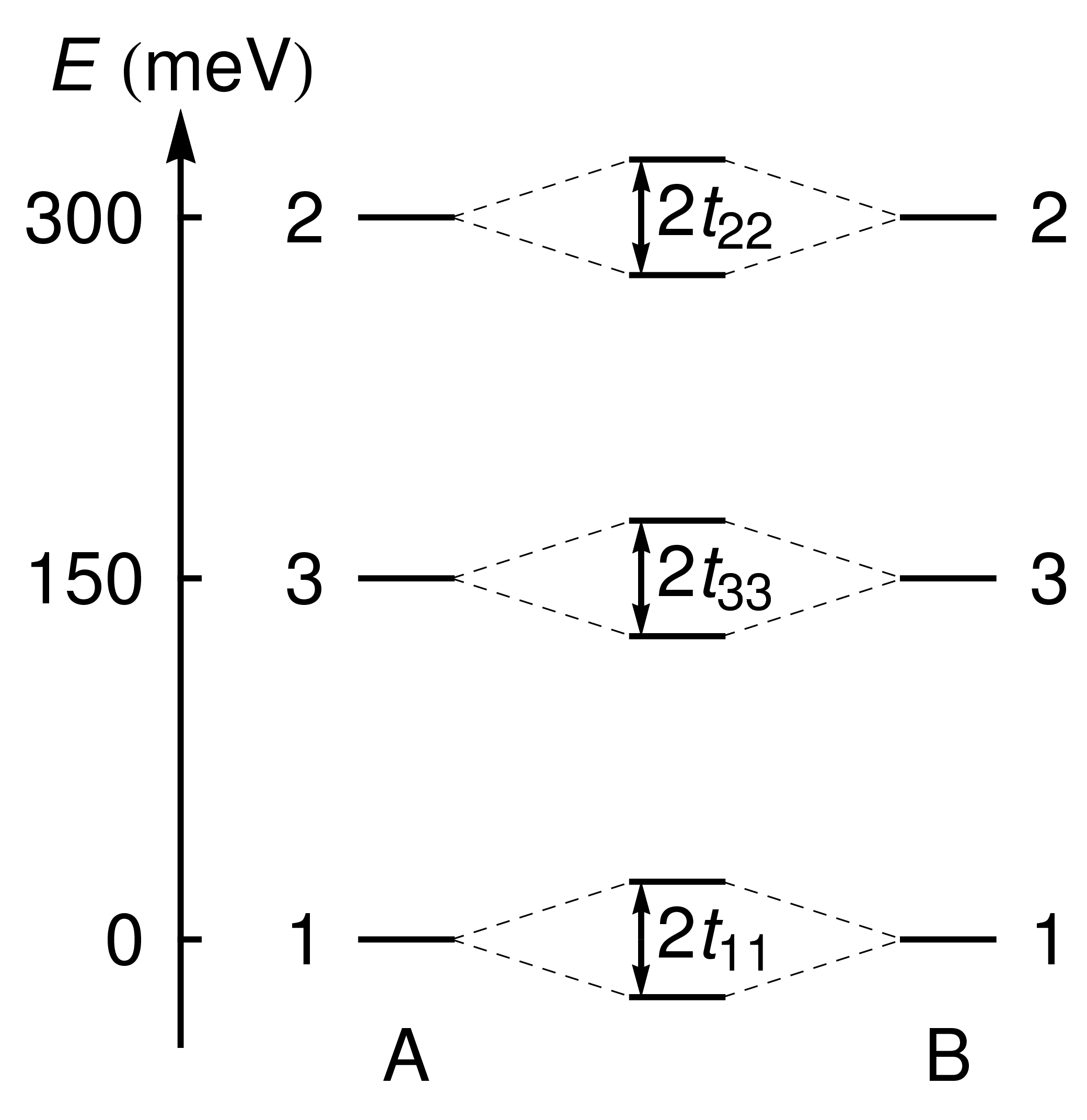
Figure 6: Hybridization of adiabatic orbitals in a two-site model.

Neglecting the $\Omega$-dependence of coefficients $U_{\mathbf{m}li}$ in Eq. (46), the eigenvalue problem for the pseudorotational nuclear wave function reduces to the equation:

$$\left(\hat{H}_{\rm rot}^{\rm nuc}+E_{\rm rot}^{\rm el}+E^{\rm el}_{0}(\Omega)\right)\chi^{\rm rot}(\Omega)=E^{\rm rot}\chi^{\rm rot}(\Omega).$$ (52)

where $E^{\rm el}_{0}(\Omega)$ is the adiabatic band energy:

$$E^{\rm el}_{0}(\Omega)=\sum_{i\sigma}^{\rm occ}\epsilon_{i}(\Omega),$$ (53)

and $E^{\rm el}_{\rm rot}$ is the expectation value of $\hat{H}^{\rm el}_{\rm rot}$, Eq. (44):

$$E^{\rm el}_{\rm rot} = \langle\Phi_{\rm S}^{\rm ad}|\hat{H}_{\rm rot}^{\rm el}|\Phi_{\rm S}^{\rm ad}\rangle.$$ (54)

The direct calculation of this matrix element gives:

$$E^{\rm el}_{\rm rot} = \sum_{\mathbf{m}}\frac{\hslash^{2}}{8q_{0}^{2}}\left(10n_{\mathbf{m}1}+10n_{\mathbf{m}2}+16n_{\mathbf{m}3}\right.$$ (55)

$$- \left.4n_{\mathbf{m}1}n_{\mathbf{m}2}-16n_{\mathbf{m}2}n_{\mathbf{m}3}-16n_{\mathbf{m}3}n_{\mathbf{m}1}\right)$$

$$+ \sum_{\mathbf{m}}\sum_{i}^{\rm occ}\frac{\hslash^{2}}{8q_{0}^{2}}\left(4\left|U_{\mathbf{m}1i}\right|^{2}\left|U_{\mathbf{m}2i}\right|^{2}\right.$$

$$+ \left.16\left|U_{\mathbf{m}2i}\right|^{2}\left|U_{\mathbf{m}3i}\right|^{2}+16\left|U_{\mathbf{m}3i}\right|^{2}\left|U_{\mathbf{m}1i}\right|^{2}\right),$$

where $n_{\mathbf{m}l}$ are populations of the adiabatic orbitals $(l)$ on the site $\mathbf{m}$. The last term is smaller than the other terms by $1/N$ because $|U_{\mathbf{m}li}|\approx 1/\sqrt{N}$ and $\sum_{i}|U_{\mathbf{m}li}|^{2}|U_{\mathbf{m}l^{\prime}i}|^{2}\approx 1/N$, while the occupation number $n_{\mathbf{m}l}=\sum_{i}|U_{\mathbf{m}li}|^{2}\approx 1$. Neglecting the last term, we obtain

$$E^{\rm el}_{\rm rot} = \sum_{\mathbf{m}}\frac{\hslash^{2}}{8q_{0}^{2}}\left(10n_{\mathbf{m}1}+10n_{\mathbf{m}2}+16n_{\mathbf{m}3}\right.$$ (56)

$$- \left.4n_{\mathbf{m}1}n_{\mathbf{m}2}-16n_{\mathbf{m}2}n_{\mathbf{m}3}-16n_{\mathbf{m}3}n_{\mathbf{m}1}\right).\quad$$

The obtained energy is additive over the sites, with one-site contributions being equivalent with the corresponding energy of an isolated C${}_{60}^{3-}$, $E_{\rm rot}^{{\rm el}(1)}=5\hslash^{2}/(4q_{0}^{2})$ (Eq. (37) in Ref. O’Brien, 1996), in the case of full disproportionation of electron density among three orbitals, $(n_{1},n_{2},n_{3})=(1,0,1/2)$ (Sec. III.2). Note the lack of $\Omega$-dependence of the energy in Eq. (56), which is the result of neglected $\Omega$-dependence of the coefficients $U_{\mathbf{m}li}$ in Eq. (46).

On the other hand, the adiabatic band energy $E_{0}^{\rm el}$ (53) is $\Omega$-dependent even if the coefficients $U_{\mathbf{m}li}$ are not, and this dependence a priori is not weak. This $\Omega$-dependence is estimated here by direct calculations of the uncorrelated band energy $E_{\rm t}^{0}$ for different directions of ordered JT distortions, $q=\sqrt{3}g$. The obtained variations of $E_{\rm t}^{0}$ do not exceed 12 meV (Fig. 7). The variation of $E_{\rm t}^{0}$ will be even smaller for disordered system because the Euler angle dependence is smeared out by the disorder. Including electron correlation effects via the Gutzwiller’s ansatz described above (Sec. III.2) will result in the case of $U=U_{c}$ (corresponding to $q=1.85$, see Fig. 4b) to a reduction of uncorrelated $E_{\rm t}^{0}$ ($\approx-240$ meV) by one order of magnitude (Fig. 4b). At the same extent will reduce the variations of the band energy in function of the direction of JT distortions, which means that they are negligible compared to the dynamical contribution to JT stabilization energy (Fig. 5).

In $A_{3}$C₆₀ crystals the JT pseudorotations after the Euler angles $\Omega$ can be also hindered by intermolecular vibrations. However, the energy of these vibrations ($\approx 5-10$ meV Gunnarsson (1997a)) is much lower than the energy gain due to delocalization of JT deformations in the trough.

Hence the vibronic dynamics is expected to be unquenched, like in insulating fullerides Cs₃C₆₀. Iwahara and Chibotaru (2013) Given the near independence of the band energy $E_{0}^{\rm el}$ on the pseudorotation coordinates of C${}_{60}^{3-}$ sites $(\Omega)$, and the full $\Omega$-independence of the contribution (56), the pseudorotational Hamiltonian (52) becomes merely a sum of on-site contributions. Each such contribution is an operator depending on $\Omega_{\mathbf{m}}$ Euler coordinates of the corresponding site, Eq. (43), which means that the pseudorotational wave function factorizes,

$$\chi^{\rm rot} = \prod_{\mathbf{m}}\chi_{\mathbf{m}}^{\rm rot}(\Omega_{\mathbf{m}}),$$ (57)

with $\chi_{\mathbf{m}}^{\rm rot}$ being eigenfunctions of one-site operators in Eq. (43). Then, taking into account the factorization of the radial part, Eq. (49), the Gutzwiller wave function with dynamical JT effect on fullerene sites has the form:

$$|\Psi_{\rm G}\rangle = \hat{P}_{\rm G}|\Phi_{\rm S}^{\rm ad}\rangle\times\prod_{\mathbf{m}}\chi_{\mathbf{m}}^{\rm rad}\chi_{\mathbf{m}}^{\rm rot},$$ (58)

and the Gutzwiller projector (19) will involve now population operators for adiabatic orbitals on the fullerene sites:

$$\hat{P}_{\rm G} = \prod_{\mathbf{m}}\exp\left(-\frac{1}{2}\sum_{l\sigma\neq l^{\prime}\sigma^{\prime}}A_{\mathbf{m}ll^{\prime}}\hat{n}_{\mathbf{m}l\sigma}\hat{n}_{\mathbf{m}l^{\prime}\sigma^{\prime}}\right).$$ (59)

(a)

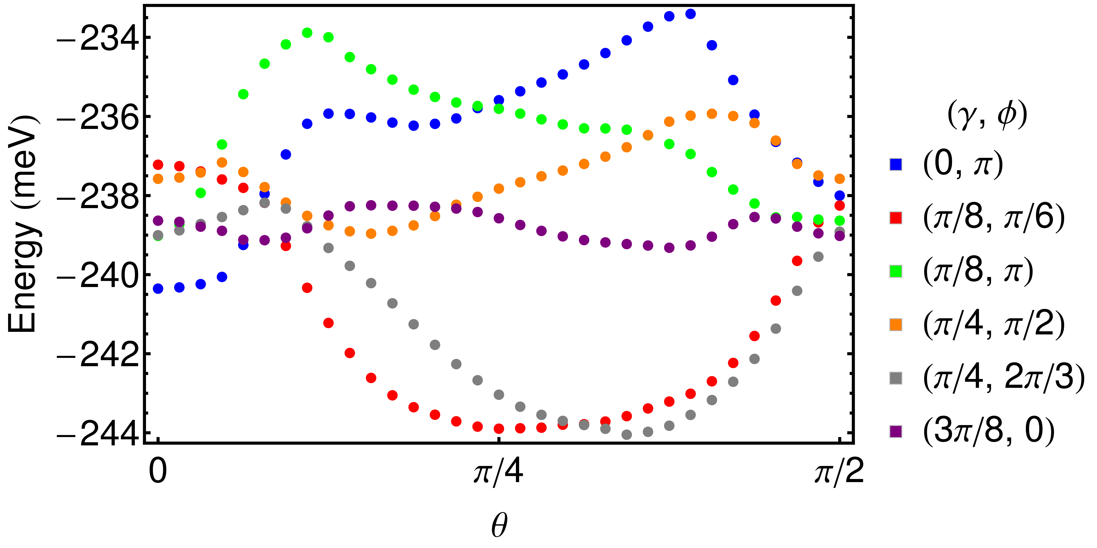
(b)

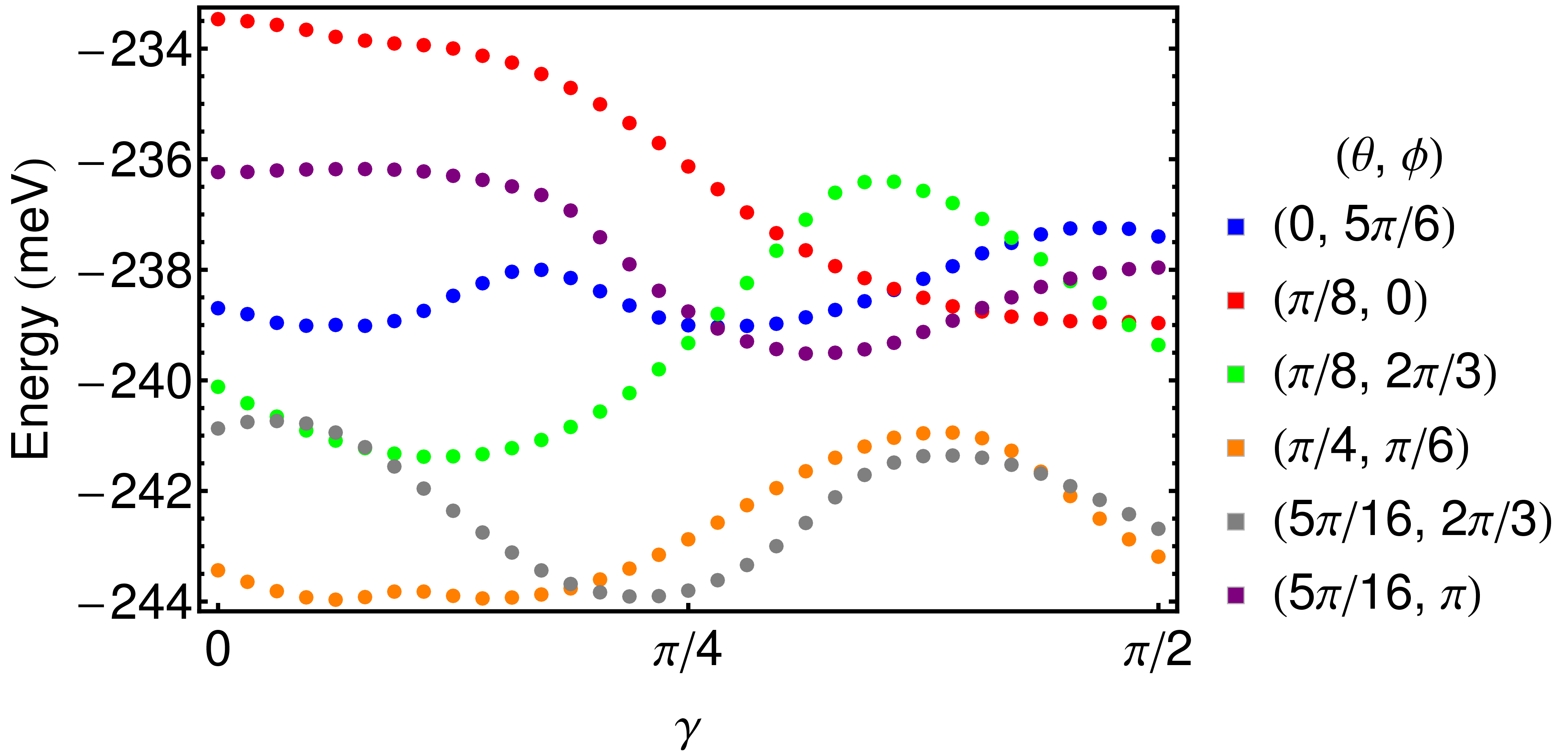
Figure 7: (color online) Dependence of uncorrelated band energy $E_{\rm t}^{0}$ on the Euler angles of JT distortions $\theta$ (a) and $\gamma$ (b), respectively, for $q=\sqrt{3}g=1.85$.

IV.3 Self-consistent Gutzwiller approach for the ground vibronic state

The ground state energy of the dynamical JT system is obtained by minimizing the total energy per site. Although the adiabatic band orbitals (46) correspond to a disordered system, this will not pose any complication if we assume that the band energy of these orbitals is independent on the form of adiabatic orbitals, i.e., on the three Euler angles characterizing the “direction” of JT distortions on sites. This seems to be indeed the case given the weak dependence of band energy on the local JT distortions established above (Fig. 7). Then the calculation of the electronic part of the energy can be done for a particular case of Euler angles equal on all sites, yielding the previous result for a translational system, while the nuclear part of the wave function (58) will give the dynamical contribution.

Hence, within the adiabatic approximation (42), the ground energy with the Gutzwiller’s wave function (58) is given by

$$E_{\rm ad} = E_{\rm t}+E_{\rm bi}-\frac{3\hslash\omega g_{\rm eff}^{2}}{2}+E_{\rm DJT}^{\rm ad},$$ (60)

where the dynamical JT deformation $q_{0}$ is replaced by

$$q_{0} = \sqrt{3}g_{\rm eff},$$ (61)

and $E_{\rm DJT}^{\rm ad}$ is the dynamical JT contribution

$$E_{\rm DJT}^{\rm ad} = -\frac{3\hslash\omega}{2}-\frac{3\hslash\omega}{8g_{\rm eff}^{2}}+E_{\rm rot}.$$ (62)

The zero-point energy of the five-dimensional harmonic oscillator is set to zero. The first and the second terms in Eq. (62) appear from the radial Hamiltonian (39) O’Brien (1996) and $E_{\rm rot}$ is the eigenvalue of the pseudorotational Hamiltonian (52). Furthermore, the dynamical contribution (62) is replaced by the exact $E_{\rm DJT}$ (Fig. 5), yielding

$$E = E_{\rm t}+E_{\rm bi}-\frac{3\hslash\omega g_{\rm eff}^{2}}{2}+E_{\rm DJT}(g_{\rm eff}).$$ (63)

The ground state for dynamical JT system is obtained by self-consistent minimization of the energy (63) with respect to $\{u_{\lambda,p\mathbf{k}}\}$ and $\{A_{\lambda\lambda^{\prime}}\}$. We obtain similar formula as Eqs. (28) and (30), with the only difference in the JT term of one-particle Hamiltonian:

$$h_{\lambda\lambda^{\prime}}^{\mathbf{k}} = q_{\lambda\lambda^{\prime}}t_{\lambda\lambda^{\prime}}^{\mathbf{k}}+\delta_{\lambda\lambda^{\prime}}\left[\sum_{\kappa\kappa^{\prime}}\frac{\partial q_{\kappa\kappa^{\prime}}}{\partial n_{\lambda}}\tau_{\kappa\kappa^{\prime}}+\frac{1}{2}\frac{\partial E_{\rm bi}}{\partial n_{\lambda}}\right.$$

$$+ \left.\left(-\frac{3\hslash\omega}{2}g_{\rm eff}+\frac{g}{2}\frac{\partial E_{\rm DJT}(g_{\rm eff})}{\partial g_{\rm eff}}\right)\left(\delta_{\lambda x}-\delta_{\lambda y}\right)\right].$$

IV.4 Dynamical Jahn-Teller instability in K₃C₆₀

(a)

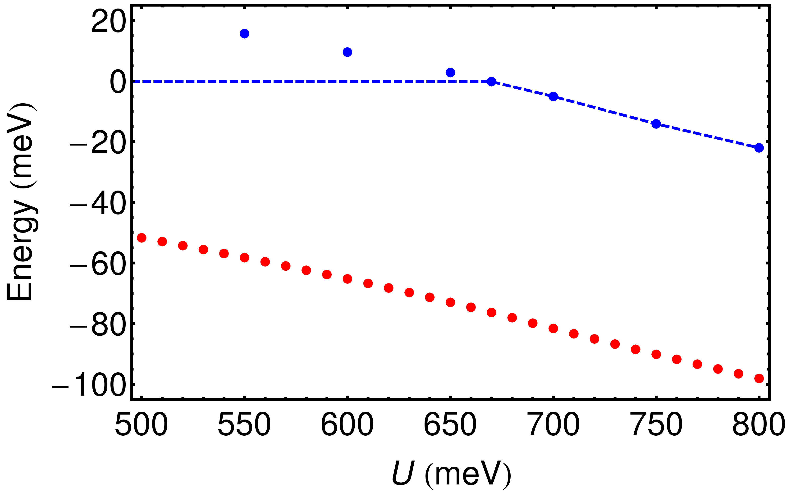
(b)

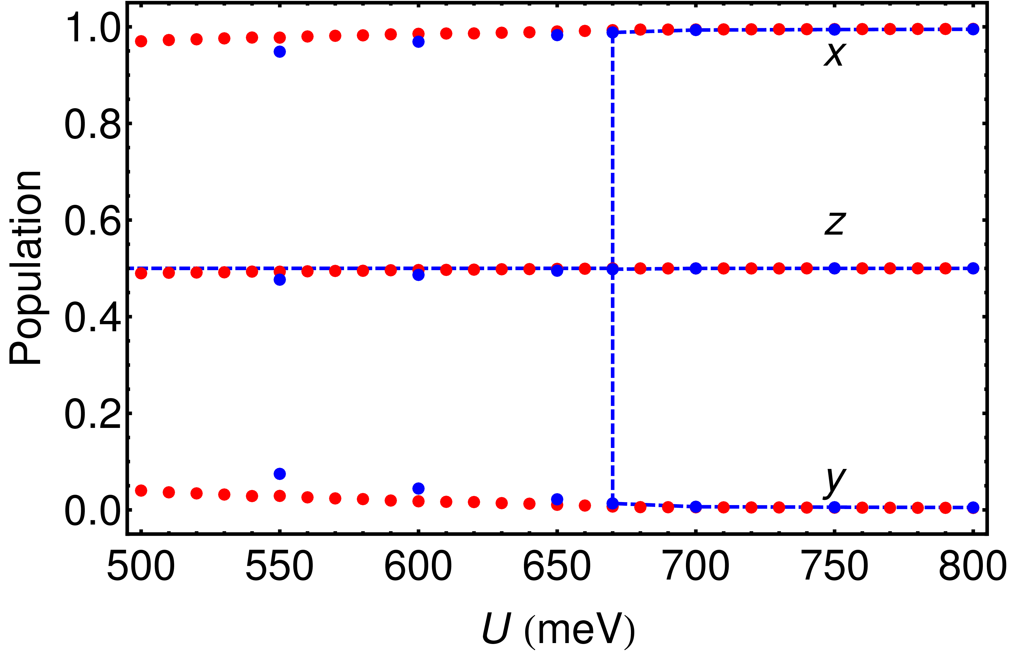
Figure 8: (color online) (a) Total energy and (b) occupation numbers of LUMO orbitals $n_{\lambda}$ with static (blue) and dynamical (red) JT effects as a function of $U$. The blue points and the dashed line correspond to the minimum with static JT distortion and the global minimum of $E_{\rm g}$, respectively. Total energy at $q=0$ is set to zero at each $U$. $x$, $y$, and $z$ in (b) are orbital components under distortion (13).

Minimizing the total energy (63), we obtain the ground energy in the presence of the JT dynamics on sites (Fig. 8a). In the case of static JT effect, the JT distortion appears for $U>670$ meV (Fig. 4a). We can see, however, that the JT dynamics enhances the dynamical JT deformation, and, consequently, the disproportionation of the occupation numbers in the adiabatic orbitals are also enhanced (Fig. 8b). As a result the critical value of electron repulsion parameter for JT instability ($U_{c}$) is significantly reduced in the dynamical case. In particular, the critical value is smaller than the estimated $U=750$ meV for K₃C₆₀, Nomura et al. (2012) hence, the metallic fullerides always exhibit dynamical JT instability in the ground state. This explains the absence of staggered JT deformations in the x-ray diffraction data of $A_{3}$C₆₀. Furthermore, since $U>U_{c}$ the equilibrium JT distortions on sites will be close to maximal possible, i.e., to their values in a free C${}_{60}^{3-}$ ion.

V Effect of electron correlation and Jahn-Teller instability on one-particle states

V.1 Orbital disproportionation

The electron correlation and the JT effect induce differences in the population of the three LUMO orbitals on fullerene sites (orbital disproportionation). Within the broken-symmetry Hartree-Fock approach, Chibotaru and Ceulemans (1996) the JT and the bielectronic energy per site is

$$E^{\rm HF} = -\frac{3\hslash\omega g_{\rm eff}^{2}}{2}+U\left(\frac{5}{12}n^{2}-\Delta n_{1}^{2}-\Delta n_{2}^{2}-\Delta n_{3}^{2}\right),$$

where $n$ is the total population of the fullerene site, $\Delta n_{l}$ is the deviation of the occupation of the orbital subband from the case of cubic symmetry $(1/2)$, and one single average electron repulsion parameter $U$ (5) is used for simplicity. The HF energy with full disproportionation, $(n_{1},n_{2},n_{3})=(1,0,1/2)$, is lower than the energy of the degenerate system $(n_{1},n_{2},n_{3})=(1/2,1/2,1/2)$ by

$$\Delta E^{\rm HF} = -\frac{3\hslash\omega g^{2}}{2}-\frac{U}{2}.$$ (66)

The orbital disproportionation is seen also in the present Gutzwiller’s treatment (Fig. 8). In terms of the electron configurations, the equal population of three LUMO bands in a cubic band structure results in their equal probability ($1/2^{6}$). The HF type symmetry breaking equally enhances the weights of four configurations, $\psi_{1}^{2}$, $\psi_{1}^{2}\psi_{3}^{1}$ (both spin projections) and $\psi_{1}^{2}\psi_{3}^{2}$, and quenches the others, leading to the gain of bielectronic energy per site $E_{\rm bi}$ by $U/2$. The weights of configurations $\psi_{1}^{2}\psi_{3}^{1}$ among the four are further enhanced and the rest of them are further reduced in the Gutzwiller treatment, which additionally lowers $E_{\rm bi}$ by $U/4$ in the limit of strong correlation. The latter becomes possible because of multi determinantal character of the Gutzwiller ansatz.

Despite the larger gain of $E_{\rm bi}$ in Gutzwiller approach compared to HF one, the latter predicts smaller $U_{c}$ for the static JT distortion. This is due to the artifactual feature of the broken-symmetry HF approach mentioned above which leads, in particular, to orbital disproportion in K₃C₆₀ without JT effect on fullerene sites. Ceulemans et al. (1997) Indeed, even in the absence of the vibronic coupling, $g=0$, the broken-symmetry HF state is more stable than the cubic band solution by $U/2$, Eq. (66). On the other hand, the Gutzwiller’s wave function is not disproportionated in the absence of JT effect, which is testified by equal population of three LUMO orbitals at $q=0$ point for arbitrary $U$ (Fig. 4c). This is the result of a higher flexibility of the Gutzwiller’s wave function, which can include various configurations without changing the bielectronic energy, such as equally populated configurations of $\psi_{1}^{1}\psi_{2}^{1}\psi_{3}^{1}$ type.

Orbital disproportionation can be directly observed in spectroscopy, e.g., in photoemission spectra of fullerides. Following the preceding discussion, the quasiparticles will belong to subbands with definite orbital index, $l=1,2,3$, separated by energy gaps (Fig. 9a). The centers of gravity of these subbands is expected to coincide with the centers of Gutzwiller subbands obtained as solutions of Eq. (28). The latter are expressed by the sum of the JT splitting and the Coulomb repulsion energy:

$$\epsilon_{{\rm bi},l} = \sum_{l^{\prime}\sigma^{\prime}(\neq l\sigma)}U\frac{\langle\Psi|\hat{n}_{\mathbf{m}l\sigma}\hat{n}_{\mathbf{m}l^{\prime}\sigma^{\prime}}|\Psi\rangle}{\langle\Psi|\hat{n}_{\mathbf{m}l\sigma}|\Psi\rangle},$$ (67)

where $\Psi$ is the ground state wave function. Consequently, the energy gap between centers of weight of the subbands is expressed as:

$$\Delta\epsilon_{\rm disp} = \frac{3\hslash\omega g_{\rm eff}^{2}}{2}+\Delta\epsilon_{\rm bi}.$$ (68)

The bielectronic part $\Delta\epsilon_{\rm bi}$ of Eq. (68) for broken-symmetry HF solution is given by $\Delta\epsilon_{\rm bi}^{\rm HF}=U/2$. Chibotaru and Ceulemans (1996); Ceulemans et al. (1997) $\Delta\epsilon_{\rm bi}$ for Gutzwiller wave function is calculated using Eq. (79). $\Delta\epsilon_{\rm bi}^{\rm HF}$ and $\Delta\epsilon_{\rm bi}$ for Gutzwiller’s wave function are shown in Fig. 9b. $\Delta\epsilon_{\rm bi}^{\rm HF}$ monotonically increases with $U$, while $\Delta\epsilon_{\rm bi}$ for the Gutzwiller’s solution approaches to zero. The bielectronic contribution $\Delta\epsilon_{\rm bi}$ becomes zero because the system approaches to the isolated molecular limit: when electrons are completely localized due to the metal-insulator transition, the splitting of the subbands reduces to the JT splitting in isolated C${}_{60}^{3-}$ ions. We can see from Fig. 9b that $\Delta\epsilon_{\rm bi}$, while exaggerated in broken-symmetry HF approach, is not an artifactual feature but, on the contrary, gives a non-negligible contribution to the splitting of quasiparticle subbands in the metallic phase. Figure 10 shows that the charge fluctuations (probabilities of configurations with $n=2,4$) is suppressed at $U\lesssim$ 700 meV, signaling the arising of metal-insulator transition.

(a)	(b)

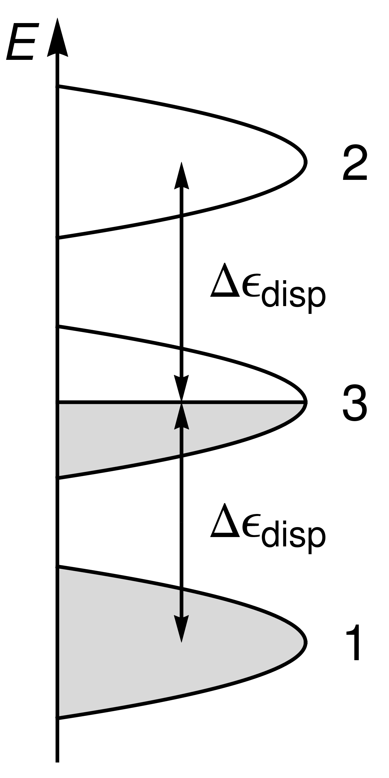
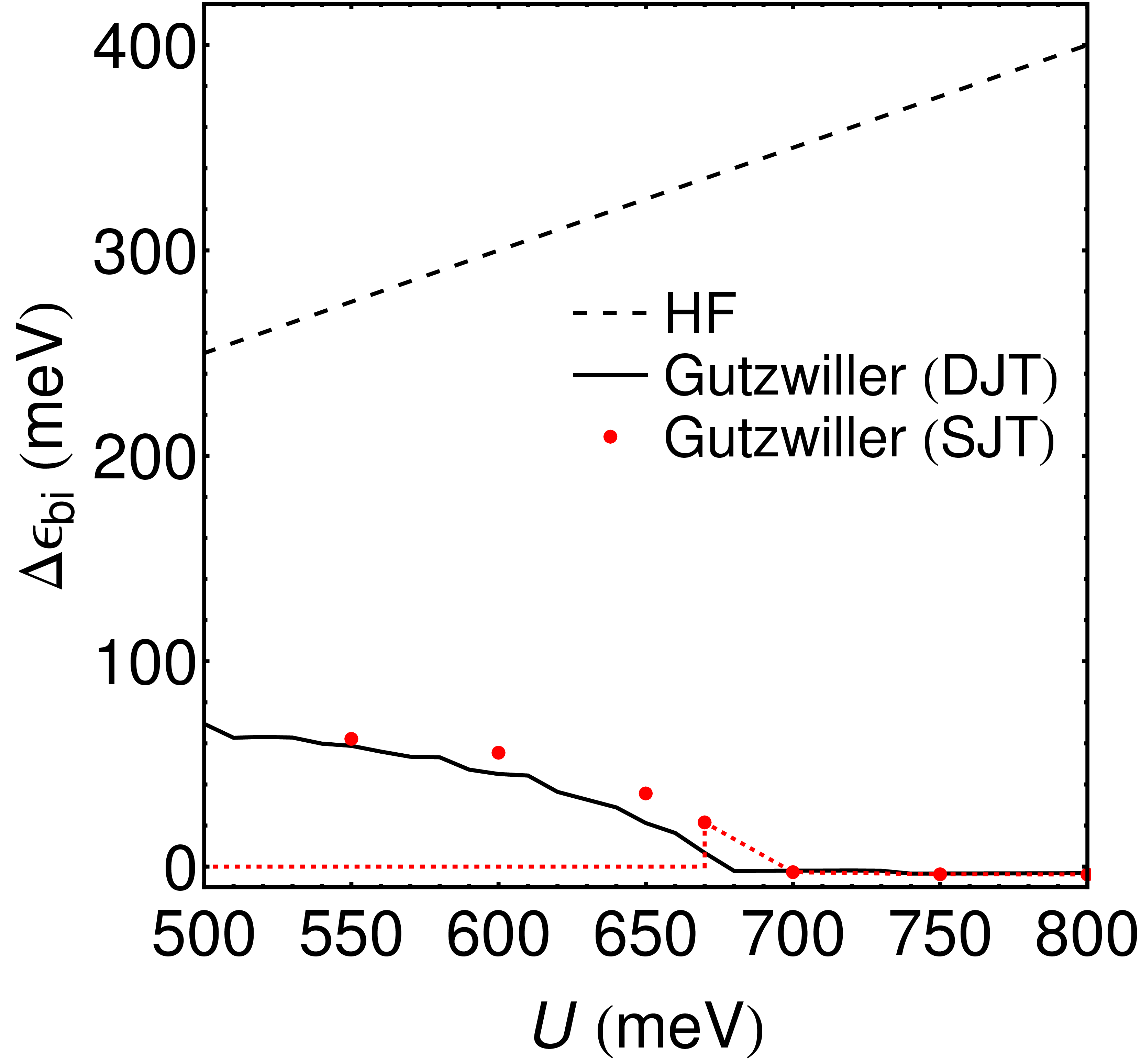
Figure 9: (color online) (a) The energy gap between Gutzwiller subbands, $\Delta\epsilon_{\rm disp}$ (68). (b) The bielectronic part $\Delta\epsilon_{\rm bi}$ of Eq. (68) as function of $U$ (meV) for HF (dashed line), Gutzwiller with dynamical JT (solid line), and Gutzwiller solution with static JT distortion (points). $\Delta\epsilon_{\rm bi}$ for the global minimum with the static JT effect is shown by the red dashed line.

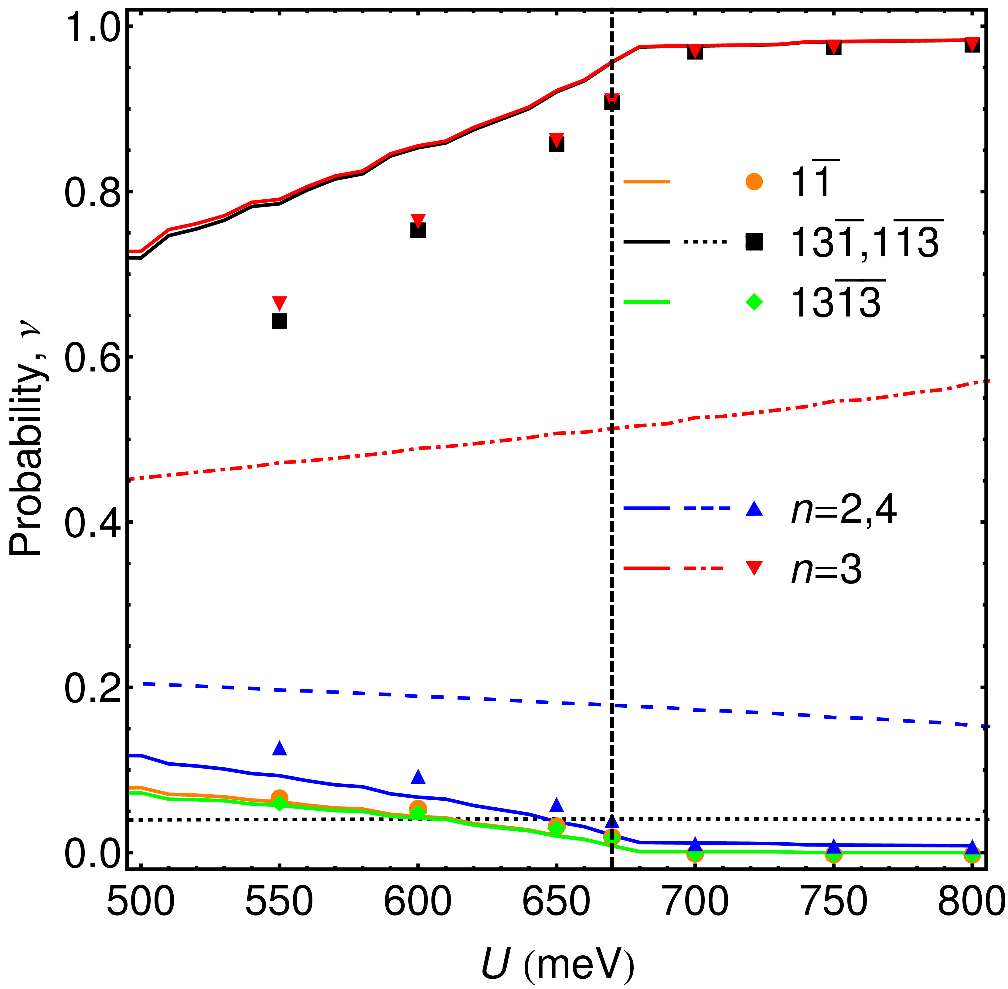
Figure 10: (color online) The probabilities of the electron configurations appearing in $\Psi_{\rm G}$, $\nu$,Vollhardt (1984); Ogawa et al. (1975) as functions of $U$. Dotted, dashed and dot-dashed lines correspond to cubic symmetry band structure, solid lines correspond to dynamic JT effect, and symbols correspond to static JT effect. Black, blue, and red indicate the electron configuration $\psi_{1}^{2}\psi_{2}^{1}$, sum of $\nu$’s over $2$ (or $4$) electron configurations, and sum of $\nu$’s over $3$ electron configurations, respectively. The vertical dashed line indicates $U_{c}$ for the static JT instability. $\nu$’s for $2$ and $4$ electrons are almost identical to each other (only the data for $n=2$ are shown). $\nu$’s for $n=0,1,5,6$ are not shown here because they are close to zero.

(a)

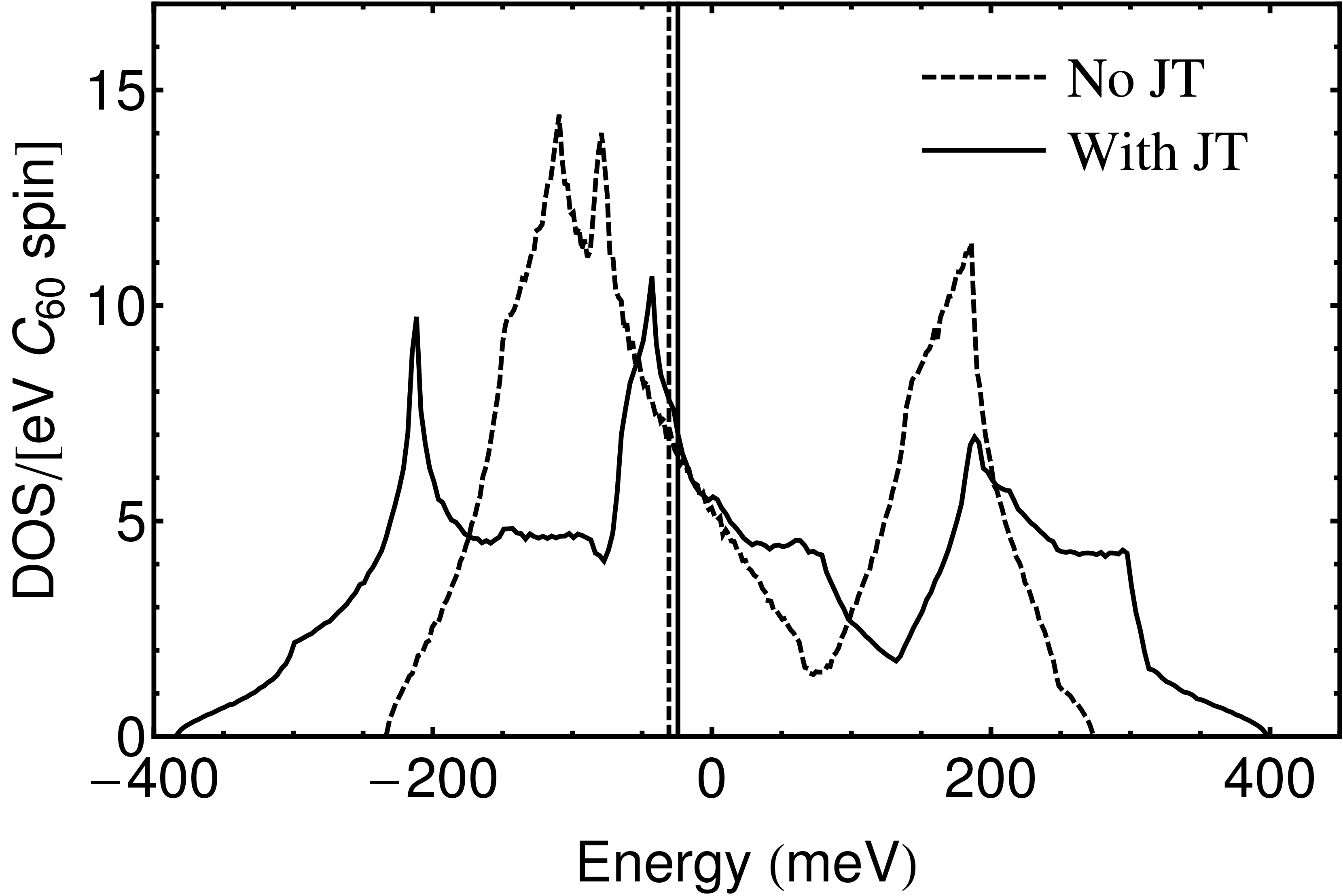
(b)

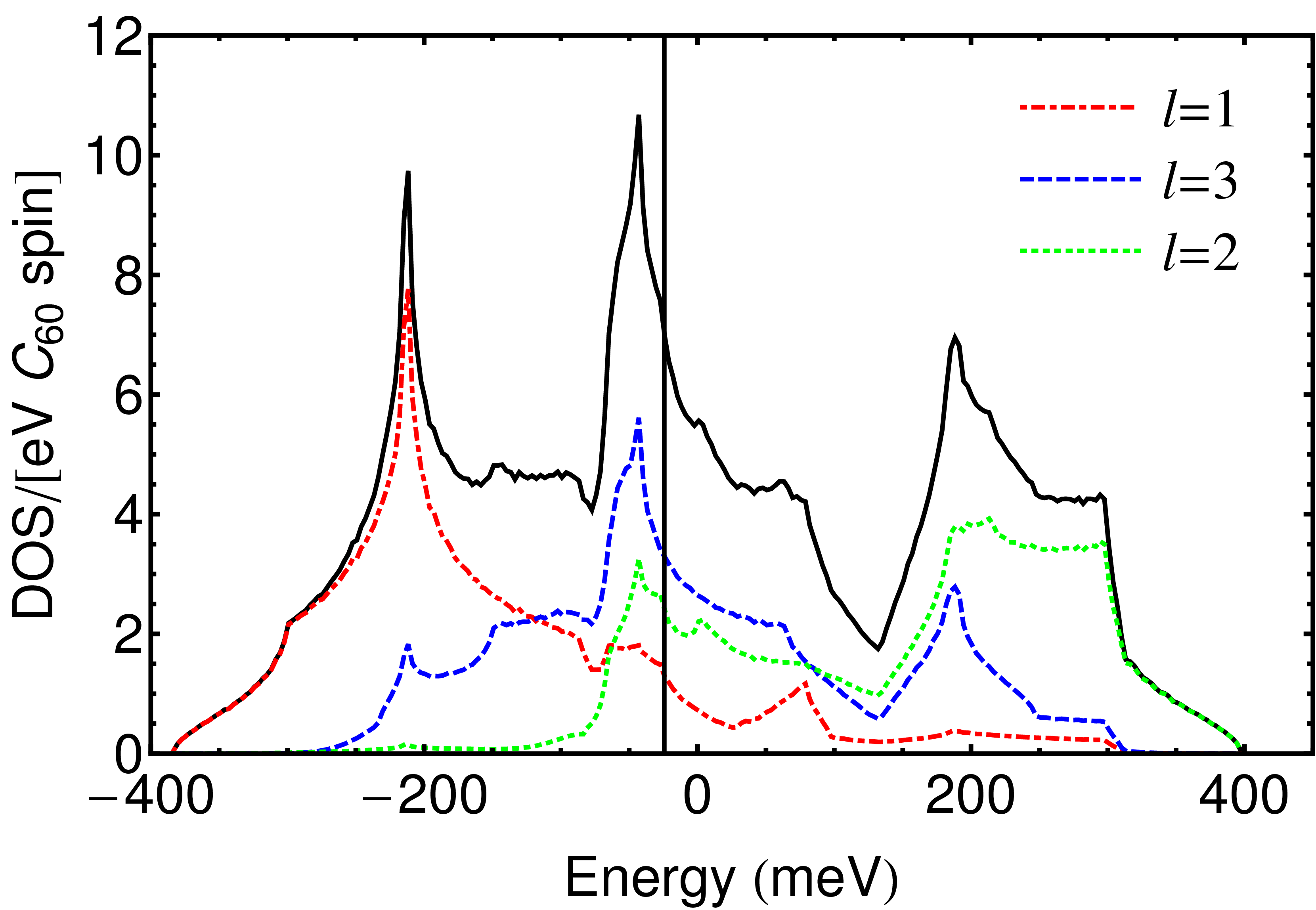
Figure 11: (color online) (a) DOS’s per C₆₀ and spin for the uncorrelated LUMO band of K₃C₆₀ in the absence (dashed) and the presence (solid) of equilibrium JT distortions on fullerene sites. (b) DOS with the JT distortion and partial DOS’s corresponding to three adiabatic orbitals. The vertical lines indicate Fermi levels.

V.2 Density of states of uncorrelated LUMO band

It is also of interest to find out how the uncorrelated band structure is affected by JT instability. Figure 11 shows the density of states (DOS) of the uncorrelated LUMO band in the presence of equilibrium JT distortion ($q=1.85$). Compared to cubic band structure, we see a strong enlargement of the bandwidth by ca 300 meV. The analysis of partial density of states shows that the degenerate LUMO band splits into three subbands (Fig. 11b) mainly contributed by one of the adiabatic orbitals (these are $x$, $y$ and $z$ for the distortion (13)). This means that the electron correlation in fullerides does not take place in a degenerate LUMO band. In particular, the Mott-Hubbard transition in cubic fullerides basically occurs in a split band structure, where half-filled is only the middle band. This calls for reconsideration of the role played by orbital degeneracy in the Mott-Hubbard transition in fullerides.

(a)

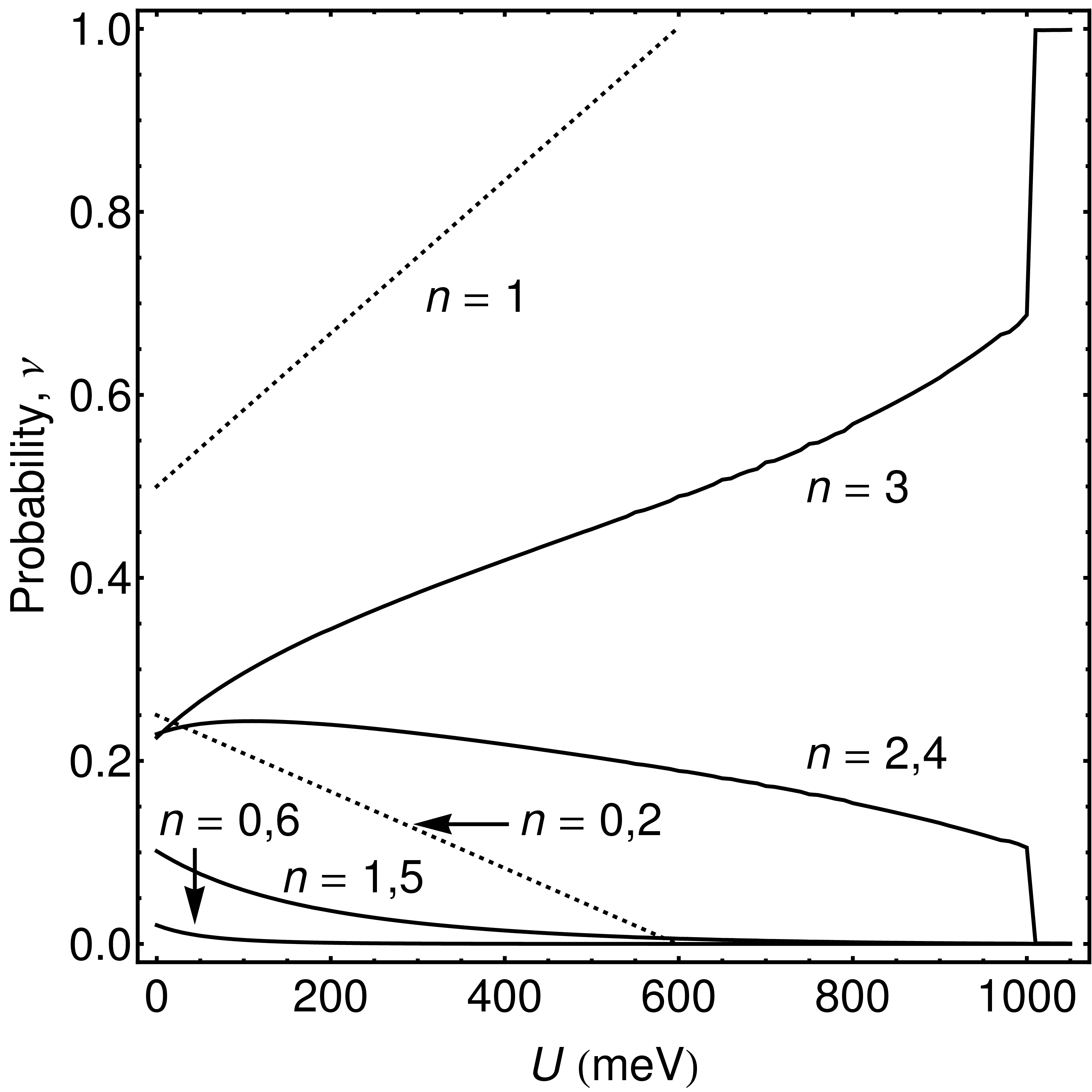
(b)

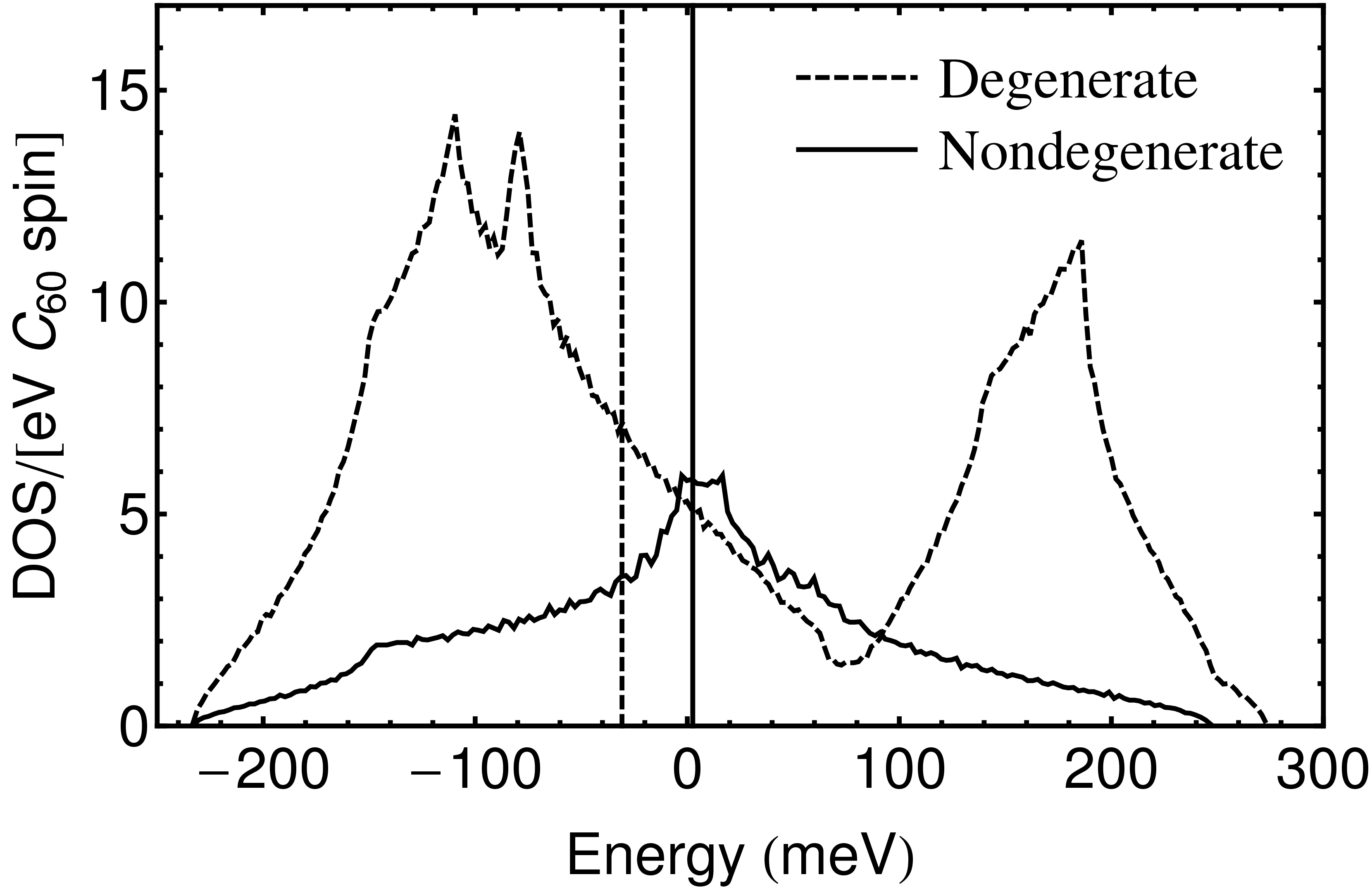
Figure 12: (a) The probabilities of the electron configurations appearing in Gutzwiller wave function of half-filled cubic system, $\nu$,Vollhardt (1984); Ogawa et al. (1975) as functions of $U$. The dashed lines and solid lines correspond to $\nu$’s for non-degenerate (one electron per site) and three-fold degenerate systems (three electrons per site), respectively. (b) The DOS’s for the non-degenerate (solid line) and degenerate (dashed line) systems. Vertical lines show the position of the corresponding Fermi levels.

VI Discussion and Conclusions

The vibronic interaction and the electron correlation in $A_{3}$C₆₀ are concomitantly treated by a new approach proposed here based on self-consistent Gutzwiller’s ansatz with orbital-specific variational parameters. The present Gutzwiller’s calculations with realistic vibronic constants, Hund’s rule coupling and parameters of the LUMO band predict that both the static and the dynamical JT deformations arise in $A_{3}$C₆₀. Since the electron correlation quenches the band energy, the localization of the electrons is enhanced, and consequently, the JT distortions on C${}_{60}^{3-}$ sites is facilitated. It is shown that the dynamical JT instability appears for smaller on-site Coulomb repulsion, $U<500$ meV than the static one (Fig. 8b). Due to the existence of the dynamical JT distortion, the adiabatic LUMO band splits into three subbands (Fig. 11). An indirect experimental evidence for the existence of dynamical JT effect in fullerides is given by NMR spectroscopy of Cs₃C₆₀, showing that features attributed to dynamical Jahn-Teller effect in its insulating phase persist when this material is brought into metallic phase by applying an external pressure. Arčon

VI.1 Correlation in split bands

The results of the present work do not support the established view that the electron correlation in fullerides takes place in a degenerate LUMO band. As was shown by Gunnarsson et al., Gunnarsson (2004) Lu Lu (1994) and Han et al. Han et al. (1998) the orbital degeneracy of the band/metal sites increases the critical ratio $U/w$ for Mott-Hubbard metal-insulator transition where $w$ is the width of the band. Gunnarsson et al. has found that this ratio is $1.5-2.5$ for $A_{3}$C₆₀, which is significantly larger than the critical ratio $U/w\approx 1$ for Mott-Hubbard transition in lattices with orbitally non-degenerate sites. Gunnarsson et al. (1996); Gunnarsson (2004) With the bandwidth $w\approx 0.5-0.6$ eV Gunnarsson (2004) (Fig. 11a) and the estimated $U\approx 1.3-1.6$ eV Antropov et al. (1992) it was natural to conclude that the orbital degeneracy of the LUMO band, leading to large critical values of $U/w$, is the reason for K₃C₆₀ and Rb₃C₆₀ to remain metals. Gunnarsson (2004) This picture has become a basis for the interpretation of metal-insulator transition in fullerides, Gunnarsson (2004); Iwasa and Takenobu (2003) in particular, in Cs₃C₆₀. Ganin et al. (2008); Takabayashi et al. (2009); Ganin et al. (2010) Contrary to that, the JT-split correlated state derived here exhibits the Mott-Hubbard transition at a lower critical ratio $U/w$. Indeed, Fig. 10 shows that the probability $n$ for $n=2,4$ configurations goes to zero at $U>$ 700 meV, signaling the localization of electron on fullerene sites. Thus we obtain a critical ratio $U/w=1.4$ which is smaller than predicted for assumed perfectly degenerate LUMO band. Gunnarsson et al. (1996); Gunnarsson (2004) This, however, does not imply automatically an insulating state for K₃C₆₀ since the upper recent estimate for $U$ in this fulleride is 750 meV, Nomura et al. (2012) and the actual value can be significantly lower as discussed below (Sec. VI.2). On the other hand, it would be incorrect to view the JT effect in the LUMO band as simply leading to its enlarging (Fig. 11b) which increases the critical $U$ within (enlarged) single-band picture. As a matter of fact, the electron correlation and the metal-insulator transition in fullerides develops mainly in the middle adiabatic subband. The role of the middle band in the Mott-Hubbard transition can be qualitatively reproduced by single-band model. The band energy of the single-band model, which includes only one of the $t_{1u}$ orbitals (the corresponding DOS is shown in Fig. 12a), is obtained as $E_{\rm t}=-74.7$ meV. Using the formula of the critical $U$ for non-degenerate band within Gutzwiller’s approximation, Vollhardt (1984) we obtain $U=8|E_{\rm t}|=598$ meV, which is close to $U\approx 700$ meV for $A_{3}$C₆₀ obtained in the present work (Fig. 10). The latter is larger than the estimate for the single-band model by about 100 meV due to the remaining hybridization of the split bands. From this analysis, one may conclude that the Mott-Hubbard transition mainly develops in the middle band.

An important issue is the accuracy of the calculated ground state energy. We used here a six parameter Gutzwiller ansatz (19) in combination with Gutzwiller approximation for the calculation of total energy (20). For comparison, Gunnarsson et al. Gunnarsson et al. (1996) used a single-parameter (conventional) Gutzwiller ansatz but calculated the total energy without approximation within variational Monte Carlo (VMC) approach. Comparison with exact results obtained for small clusters of C₆₀ via exact diagonalization has shown that VMC reproduce the exact total energy with accuracy of 0.1 $\%$ (see Table 7.1 in Ref. Gunnarsson, 2004), i.e., few meV of the total energy per one C₆₀ in fullerides. The deviation from exact total energy will be certainly larger in the case of Gutzwiller approximation applied here, however, it will not cover the gain of the total energy due to JT splitting/orbital disproportionation amounting many tens of meV (Fig. 5a). Thus the main conclusion concerning dynamical JT instability in fullerides seems to be unaffected by this approximation. This is further corroborated by the fact that the Gutzwiller wave function used in the present work is more flexible in variational sense than in the conventional Gutzwiller ansatz. Indeed, even in the case of degenerate LUMO band, conforming to cubic symmetry, the ansatz (19) involves two projection parameters. These are $A_{11}$ controlling the population of configurations $n_{\mathbf{m}\lambda\sigma}n_{\mathbf{m}\lambda-\sigma}$, and $A_{12}$ controlling the population of configurations $n_{\mathbf{m}\lambda\sigma}n_{\mathbf{m}\lambda^{\prime}\sigma^{\prime}}$, $\lambda\neq\lambda^{\prime}$. That these are the only independent parameters allowed by the cubic symmetry can be understood if one generalizes the form (19) to arbitrary LUMO basis on fullerene sites. Although, in general, $n_{\mathbf{m}\lambda\sigma}$ in Eq. (19) are replaced by elements of one-particle density matrix, only the diagonal remains nonzero because of the cubic symmetry. The terms in exponential of Eq. (19) then become of the form $A_{\alpha\alpha\beta\beta}n_{\mathbf{m}\alpha\sigma}n_{\mathbf{m}\beta\sigma^{\prime}}$, in which the “elasticity” tensors $A_{\alpha\alpha\beta\beta}$ will be characterized by only two independent parameters in the case of cubic symmetry. Landau and Lifshitz (1986) The second variational parameter in the Gutzwiller wave function changes drastically the description of Mott-Hubbard transition in the cubic band. Thus, in a conventional single-parameter Gutzwiller ansatz within the Gutzwiller approximation the critical $U/w=4$ in the case of threefold orbital degeneracy of sites. Lu (1994) This critical ratio is reduced to 2 in the case of Gutzwiller ansatz applied here (Fig. 12b) which is much closer to values obtained by Monte Carlo treatment. Gunnarsson et al. (1996); Gunnarsson (2004) It would be of interest to use in future the Gutzwiller ansatz for static and dynamic JT effect on sites proposed here as a trial functions in variational (VMC) and diffusion (projection) Monte Carlo (DMC) methods Gunnarsson (2004) which give more accurate description of ground state energy.

VI.2 Parameters of the LUMO model

Another important aspect concerns the values of relevant parameters for the model description of LUMO band in fullerides. Given the large number of such parameters, their accurate knowledge is of primary importance for realistic description of electronic properties of fullerides. Recently, it was proven that the DFT calculated vibronic constants of C${}_{60}^{-}$ with a hybrid B3LYP functional compare well with those extracted from photoemission spectroscopy. Iwahara et al. (2010) Then the vibronic constants for the C${}_{60}^{3-}$ anion and the exchange parameter calculated within the same DFT functional should be reliable as well. Concerning the transfer Hamiltonian, the parameters of nearest-neighbor and next-nearest-neighbor tight-binding model (Table 1) reproduce well the dispersion of the LUMO bands calculated within LDA (generalized gradient approximation, GGA) (Fig. 13). It was shown by GW calculation that the interband electronic interaction can enhance the LUMO ($t_{1u}$) bandwidth in fullerites by 30 % Shirley and Louie (1993) while the intraband interaction reduces the LUMO bandwidth in $A_{3}$C₆₀. Gunnarsson (1997b) However, in the latter case the GW approximation is ill-defined due to strong correlation effects in the LUMO band. Aryasetiawan et al. (2004); Gunnarsson (2004)

The parameter assessed with less certainty in the model Hamiltonian (1)-(4) is the intra-fullerene electron repulsion $U_{\parallel}$. Recent calculations of this parameter by constrained random-phase approximation (cRPA) Aryasetiawan et al. (2004) with GGA band energies and wave functions give in the low-frequency limit $U_{\parallel}\lesssim$ 1 eV for the series of $A_{3}$C₆₀, the smallest being $U_{\parallel}=820$ meV for K₃C₆₀. Nomura et al. (2012) It is interesting to note that the estimated $U_{\parallel}$ in Ref. Nomura et al., 2012 gives for all fullerides values $\lesssim$ 1 eV, while former estimations made for fullerite (pure C₆₀ crystal) give larger values. Gunnarsson (2004); Antropov et al. (1992); Lof et al. (1992) This is explained by the fact that in $A_{3}$C₆₀ fullerides the LUMO Wannier orbitals occupy larger volume due to hybridization with alkali atoms. Nomura et al. (2012) In these calculations a non-interacting polarization function was used that excluded polarization processes within the LUMO band. Including the latter, i.e., considering the full screening in the non-interacting metallic regime, Aryasetiawan et al. (2004) further reduces $U_{\parallel}$ by ca one order of magnitude in the low frequency limit. Nomura et al. (2012) A similar strong effect of metallic screening (arising from the LUMO band) was predicted also for a simplified treatment of metallic polarization. Chakravarty et al. (1991); Lammert et al. (1995) One should note that RPA is generally not expected to perform well in the limit of strong correlation, as well as the GW approximation mentioned above. To check the screening capability of the correlated LUMO band, Koch et al. Koch et al. (1999) did VMC and DMC calculations of an induced charge arising in response to a test charge for a threefold degenerate LUMO model of $A_{3}$C₆₀. They found that RPA performs surprisingly well till $U/w\lesssim$ 2, and even at the point of Mott-Hubbard transition (corresponding to $U/w\approx 2.5$ in their model), when the LUMO electrons become localized, the screening charge is reduced by not more than 40 % with respect to RPA screening charge calculated for non-correlated LUMO band (Fig. 2 in Ref. Koch et al., 1999). At the same extent is expected to be reduced the screening of the electron repulsion parameter by the intra-LUMO band interaction, which means that this screening is significant in the entire metallic phase of fullerides and should be taken into account for realistic assessment of $U_{\parallel}$. A rigorous model for the LUMO band, in which other degrees of freedom are excluded, requires frequency-dependent electron repulsion parameters. Aryasetiawan et al. (2004) From it an effective static Hubbard model (involving a frequency-independent $U$) can be derived by fitting the self-energy in a low-frequency domain, not exceeding the width of uncorrelated LUMO band. Aryasetiawan et al. (2004) Note that the derivations of the static $U_{\parallel}$, $U_{\perp}$ in Eq. (4) should be done self-consistently with the derivation of the ground state following the iterative equations (28)-(30).

Experimentally $U$ can be assessed from Auger spectroscopy. Lof et al. (1992); Brühwiler et al. (1993) The estimates are 1.4 $\pm$ 0.2 eV for pure C₆₀ and band insulator K₆C₆₀, Brühwiler et al. (1993) and 0.6 $\pm$ 0.3 eV for metallic K₃C₆₀. The much smaller value of $U$ in K₃C₆₀ reflects most probably the additional strong screening from half-filled LUMO band. An instructive example of the sensitivity of $U$ on intra LUMO-band screening is offered by non-cubic fullerides NH₃K₃C₆₀ Rosseinsky et al. (1993) and (CH₃NH₂)K₃C₆₀. Ganin et al. (2006) Contrary to the parent K₃C₆₀ fulleride, which is a metal, these compounds are antiferromagnetic Mott-Hubbard insulators. The main effect of spacers, NH₃ and CH₃NH₂, respectively, is the removal of degeneracy of three LUMO orbitals on fullerene sites, which apparently reduces the orbital $U/w$ from its value in cubic K₃C₆₀ predicted for threefold degenerate LUMO band, Gunnarsson et al. (1996); Gunnarsson (2004) causing the Mott-Hubbard transition. Manini et al. Manini et al. (2002) have checked this possibility via DMFT calculations of a model twofold degenerate band and found that the calculated splitting of the $t_{1u}$ orbitals is indeed sufficient to induce the Mott-Hubbard transition. However, the persistence of strong JT distortions in metallic fullerides, established in this work, calls for another interpretation. The crystal anisotropy induced by the spacers will enhance the splitting of the LUMO bands (Fig. 11b) thus reducing the intra-LUMO band screening of electron repulsion. This results in the increase of $U_{\parallel}$ and $U_{\perp}$ in Eq. (4), which is the reason why the non-cubic fullerides are Mott-Hubbard insulators.

To conclude this part, several theoretical arguments and relevant experimental data argue in the favor of non-negligible intra-LUMO band screening of Hubbard $U$ parameter, which is thus expected to be well below 1 eV. The latter is also a necessary condition for metallicity of fullerides in the presence of strong JT distortions (Fig. 10).

VI.3 Polaronic effects

The simple form of dynamical vibronic wave function (58) was derived under two simplifying assumptions. First, the polaronic effect was neglected which seems to be justified for fullerides. Indeed, while the static JT energy of C${}_{60}^{2-}$ and C${}_{60}^{4-}$ is larger than in C${}_{60}^{3-}$ by an amount $E_{\rm JT}^{(1)}=\hslash\omega g^{2}/2=50.2$ meV, the difference in the gain is compensated by the loss of stabilization energy from the dynamical contribution. In the strong vibronic coupling limit, the dynamical JT contribution of C${}_{60}^{3-}$ is $3\hslash\omega/2$ and that of C${}_{60}^{2-}$ and C${}_{60}^{4-}$ is $\hslash\omega$ because the trough is three-dimensional in the former case and two-dimensional in the latter. Then $1/3$ of the dynamical contribution of C${}_{60}^{3-}$ is lost if JT relaxation accompanies the electron transfer. Using the data from the numerical diagonalizations, the loss of the dynamical JT contribution is estimated as $-E_{\rm DJT}/3\approx 30$ meV. Therefore, the binding energy of JT polaron (the energy gain arising from full JT relaxation) is $\Delta E=-E_{\rm JT}^{(1)}-E_{\rm DJT}/3\approx-20$ meV. Compared with the total JT stabilization energy of $\approx 240$ meV the JT polaronic effect appears to be small. One should take into account that the JT polaronic effect is accompanied by the Franck-Condon reduction of the band energy, which means that the JT polaron will only show up when the band energy is reduced by correlation effects under 20 meV, i.e., close to Mott-Hubbard transition. On the other hand the stabilization energy of one electron after total symmetric fullerene distortions does not exceed 20 meV, i.e., is negligible either. Iwahara et al. (2010) In these estimations the relaxation due to displacements of alkali atoms has not been included, which is unimportant for $A_{3}$C₆₀ but can be significant in insulating $A_{4}$C₆₀ and A₆C₆₀. Wehrli et al. (2004) As for the second assumption of weak hybridization of the bands belonging to different $t_{1u}$ orbitals (Fig. 6), it seems to be only justified in the strongly correlated limit. When it is not the case, the $\Omega$-dependence of the coefficients $U_{\mathbf{m}li}$ in Eq. (46) cannot be neglected and ultimately the rotations of JT deformation on different fullerene sites (Eq. (57)) cannot be separated. This means that in metallic Cs₃C₆₀ the rotation of JT deformations occurs independently on different fullerene sites, while in K₃C₆₀ these rotations are more probable to be correlated. In the latter case the wave function (58) does not represent a close solution and should be rather considered as a variational function which nevertheless will correspond to lower total energy than the static JT solution (16).

VI.4 Summary

The main achievements of this work can be summarized as follows:

1. We have developed an approach for the investigation of correlated JT metals based on self-consistent Gutzwiller approximation.

2. The concomitant treatment of JT effect and electron correlation in metallic fullerides $A_{3}$C₆₀ proves the existence of dynamical JT instability in their ground state. The JT distortions arise due to strong reduction of the band energy by electron correlation effects and achieve an amplitude close to the value in a free C${}_{60}^{3-}$ ion.

3. The JT instability induces strong overall enlargement of the uncorrelated LUMO band and its splitting in three components corresponding to individual adiabatic orbitals on fullerene sites. The results call for reconsideration of the role played by orbital degeneracy in the physics of metallic fullerides.

4. JT distortions together with electron correlation induce disproportionation of electron density between subbands corresponding to different adiabatic orbitals on fullerene sites. Besides the JT splitting there is also a bielectronic contribution to the separation of these subbands which vanishes in the limit of strong correlation. Importantly, the orbital disproportionation does not exist as a pure electronic low-symmetry instability in the absence of JT effect on fullerene sites ($g=0$), in which case the correlated LUMO band will have a perfect cubic symmetry for any $U$.

Finally, we note that a similar analysis can be applied to other correlated metals with JT active sites.

Appendix A Tight-binding parametrization of the LUMO band structure of K₃C₆₀

We assume that all C₆₀’s in fcc K₃C₆₀ lattice are equally orientated in a similar fashion shown in Figure 1 (Fig. 3). Using the unit vectors of fcc lattice,

$$\mathbf{a}_{1} = \frac{a}{2}\left(\mathbf{e}_{y}+\mathbf{e}_{z}\right),\qquad\mathbf{a}_{2}=\frac{a}{2}\left(\mathbf{e}_{z}+\mathbf{e}_{x}\right),$$

$$\mathbf{a}_{3} = \frac{a}{2}\left(\mathbf{e}_{x}+\mathbf{e}_{y}\right),$$ (69)

the displacements $\Delta\mathbf{m}$ of the nearest neighbor sites from site $\mathbf{m}$ are written as

$$\Delta\mathbf{m} = \left(\mathbf{a}_{3},\mathbf{a}_{1}-\mathbf{a}_{2},-\mathbf{a}_{3},-(\mathbf{a}_{1}-\mathbf{a}_{2}),\right.$$ (70)

$$\left.\mathbf{a}_{1},\mathbf{a}_{2}-\mathbf{a}_{3},-\mathbf{a}_{1},-(\mathbf{a}_{2}-\mathbf{a}_{3}),\right.$$

$$\left.\mathbf{a}_{2},\mathbf{a}_{3}-\mathbf{a}_{1},-\mathbf{a}_{2},-(\mathbf{a}_{3}-\mathbf{a}_{1})\right).$$

The next nearest neighbors are displaced by vectors

$$\Delta\mathbf{m} = a\left(\mathbf{e}_{x},-\mathbf{e}_{x},\mathbf{e}_{y},-\mathbf{e}_{y},\mathbf{e}_{z},-\mathbf{e}_{z}\right).$$ (71)

Here, $a$ is the lattice constant of a simple cubic lattice and $\mathbf{e}_{x},\mathbf{e}_{y},\mathbf{e}_{z}$ correspondingly are unit vectors directed along tetragonal $x,y,z$ axes (Fig. 3). The tight-binding Hamiltonian has the form:

$$\hat{H}_{\rm t} = \sum_{\mathbf{m}}\sum_{\lambda\sigma}\epsilon\hat{n}_{\mathbf{m}\lambda\sigma}+\sum_{\mathbf{m}}\sum_{\sigma}\left(\hat{H}_{\mathbf{m}\sigma}^{\rm nn}+\hat{H}_{\mathbf{m}\sigma}^{\rm nnn}\right),$$ (72)

where the nearest-neighbor part is

$$\hat{H}_{\mathbf{m}\sigma}^{\rm nn} = t_{1}\left[\sum_{i=1}^{4}\hat{c}_{\mathbf{m}+\Delta\mathbf{m}_{i}x\sigma}^{\dagger}\hat{c}_{\mathbf{m}x\sigma}+\sum_{i=5}^{8}\hat{c}_{\mathbf{m}+\Delta\mathbf{m}_{i}y\sigma}^{\dagger}\hat{c}_{\mathbf{m}y\sigma}\right.$$

$$+ \left.\sum_{i=9}^{12}\hat{c}_{\mathbf{m}+\Delta\mathbf{m}_{i}z\sigma}^{\dagger}\hat{c}_{\mathbf{m}z\sigma}\right]$$

$$+ t_{3}\left[\sum_{i=1}^{4}\hat{c}_{\mathbf{m}+\Delta\mathbf{m}_{i}y\sigma}^{\dagger}\hat{c}_{\mathbf{m}y\sigma}+\sum_{i=5}^{8}\hat{c}_{\mathbf{m}+\Delta\mathbf{m}_{i}z\sigma}^{\dagger}\hat{c}_{\mathbf{m}z\sigma}\right.$$

$$+ \left.\sum_{i=9}^{12}\hat{c}_{\mathbf{m}+\Delta\mathbf{m}_{i}x\sigma}^{\dagger}\hat{c}_{\mathbf{m}x\sigma}\right]$$

$$+ t_{4}\left[\sum_{i=1}^{4}\hat{c}_{\mathbf{m}+\Delta\mathbf{m}_{i}z\sigma}^{\dagger}\hat{c}_{\mathbf{m}z\sigma}+\sum_{i=5}^{8}\hat{c}_{\mathbf{m}+\Delta\mathbf{m}_{i}x\sigma}^{\dagger}\hat{c}_{\mathbf{m}x\sigma}\right.$$

$$+ \left.\sum_{i=9}^{12}\hat{c}_{\mathbf{m}+\Delta\mathbf{m}_{i}y\sigma}^{\dagger}\hat{c}_{\mathbf{m}y\sigma}\right]$$

$$- t_{2}\left[\sum_{i=1}^{4}(-1)^{i}\left(\hat{c}_{\mathbf{m}+\Delta\mathbf{m}_{i}x\sigma}^{\dagger}\hat{c}_{\mathbf{m}y\sigma}\hat{c}_{\mathbf{m}+\Delta\mathbf{m}_{i}y\sigma}^{\dagger}\hat{c}_{\mathbf{m}x\sigma}\right)\right.$$

$$+ \left.\sum_{i=5}^{8}(-1)^{i}\left(\hat{c}_{\mathbf{m}+\Delta\mathbf{m}_{i}y\sigma}^{\dagger}\hat{c}_{\mathbf{m}z\sigma}+\hat{c}_{\mathbf{m}+\Delta\mathbf{m}_{i}z\sigma}^{\dagger}\hat{c}_{\mathbf{m}y\sigma}\right)\right.$$

$$+ \left.\sum_{i=9}^{12}(-1)^{i}\left(\hat{c}_{\mathbf{m}+\Delta\mathbf{m}_{i}z\sigma}^{\dagger}\hat{c}_{\mathbf{m}x\sigma}+\hat{c}_{\mathbf{m}+\Delta\mathbf{m}_{i}x\sigma}^{\dagger}\hat{c}_{\mathbf{m}z\sigma}\right)\right],$$

and the next-nearest-neighbor part is

$$\hat{H}_{\mathbf{m}\sigma}^{\rm nnn} = t_{5}\left(\hat{c}_{\mathbf{m}+a\mathbf{e}_{x}x\sigma}\hat{c}_{\mathbf{m}x\sigma}+\hat{c}_{\mathbf{m}-a\mathbf{e}_{x}x\sigma}\hat{c}_{\mathbf{m}x\sigma}\right.$$ (74)

$$+ \left.\hat{c}_{\mathbf{m}+a\mathbf{e}_{y}y\sigma}\hat{c}_{\mathbf{m}y\sigma}+\hat{c}_{\mathbf{m}-a\mathbf{e}_{y}y\sigma}\hat{c}_{\mathbf{m}y\sigma}\right.$$

$$+ \left.\hat{c}_{\mathbf{m}+a\mathbf{e}_{z}z\sigma}\hat{c}_{\mathbf{m}z\sigma}+\hat{c}_{\mathbf{m}-a\mathbf{e}_{z}z\sigma}\hat{c}_{\mathbf{m}z\sigma}\right)$$

$$+ t_{6}\left(\hat{c}_{\mathbf{m}+a\mathbf{e}_{x}y\sigma}\hat{c}_{\mathbf{m}y\sigma}+\hat{c}_{\mathbf{m}-a\mathbf{e}_{x}y\sigma}\hat{c}_{\mathbf{m}y\sigma}\right.$$

$$+ \left.\hat{c}_{\mathbf{m}+a\mathbf{e}_{y}z\sigma}\hat{c}_{\mathbf{m}z\sigma}+\hat{c}_{\mathbf{m}-a\mathbf{e}_{y}z\sigma}\hat{c}_{\mathbf{m}z\sigma}\right.$$

$$+ \left.\hat{c}_{\mathbf{m}+a\mathbf{e}_{z}x\sigma}\hat{c}_{\mathbf{m}x\sigma}+\hat{c}_{\mathbf{m}-a\mathbf{e}_{z}x\sigma}\hat{c}_{\mathbf{m}x\sigma}\right)$$

$$+ t_{7}\left(\hat{c}_{\mathbf{m}+a\mathbf{e}_{x}z\sigma}\hat{c}_{\mathbf{m}z\sigma}+\hat{c}_{\mathbf{m}-a\mathbf{e}_{x}z\sigma}\hat{c}_{\mathbf{m}z\sigma}\right.$$

$$+ \left.\hat{c}_{\mathbf{m}+a\mathbf{e}_{y}x\sigma}\hat{c}_{\mathbf{m}x\sigma}+\hat{c}_{\mathbf{m}-a\mathbf{e}_{y}x\sigma}\hat{c}_{\mathbf{m}x\sigma}\right.$$

$$+ \left.\hat{c}_{\mathbf{m}+a\mathbf{e}_{z}y\sigma}\hat{c}_{\mathbf{m}y\sigma}+\hat{c}_{\mathbf{m}-a\mathbf{e}_{z}y\sigma}\hat{c}_{\mathbf{m}y\sigma}\right),$$

In Eq. (LABEL:Eq:Htnn), $\Delta\mathbf{m}_{i}$ indicates $i$th nearest neighbor.

The DFT calculation of the band structure of K₃C₆₀ was performed using Quantum ESPRESSO 3.0 package with the pseudopotentials C.pbe-mt gipaw.UPF and K.pbe-mt fhi.UPF. Giannozzi et al. (2009) The lattice constant of K₃C₆₀ was taken from Ref. Stephens et al., 1991 and the structure of C₆₀ of Ref. Iwahara et al., 2010 was used.

The band structures from the DFT calculation (red) and the fitted tight-binding Hamiltonian (blue) are shown in Fig. 13. The transfer parameters derived from the DFT calculation are tabulated in Table 1. The present values are close to the recent estimates with optimized structure. Nomura et al. (2012)

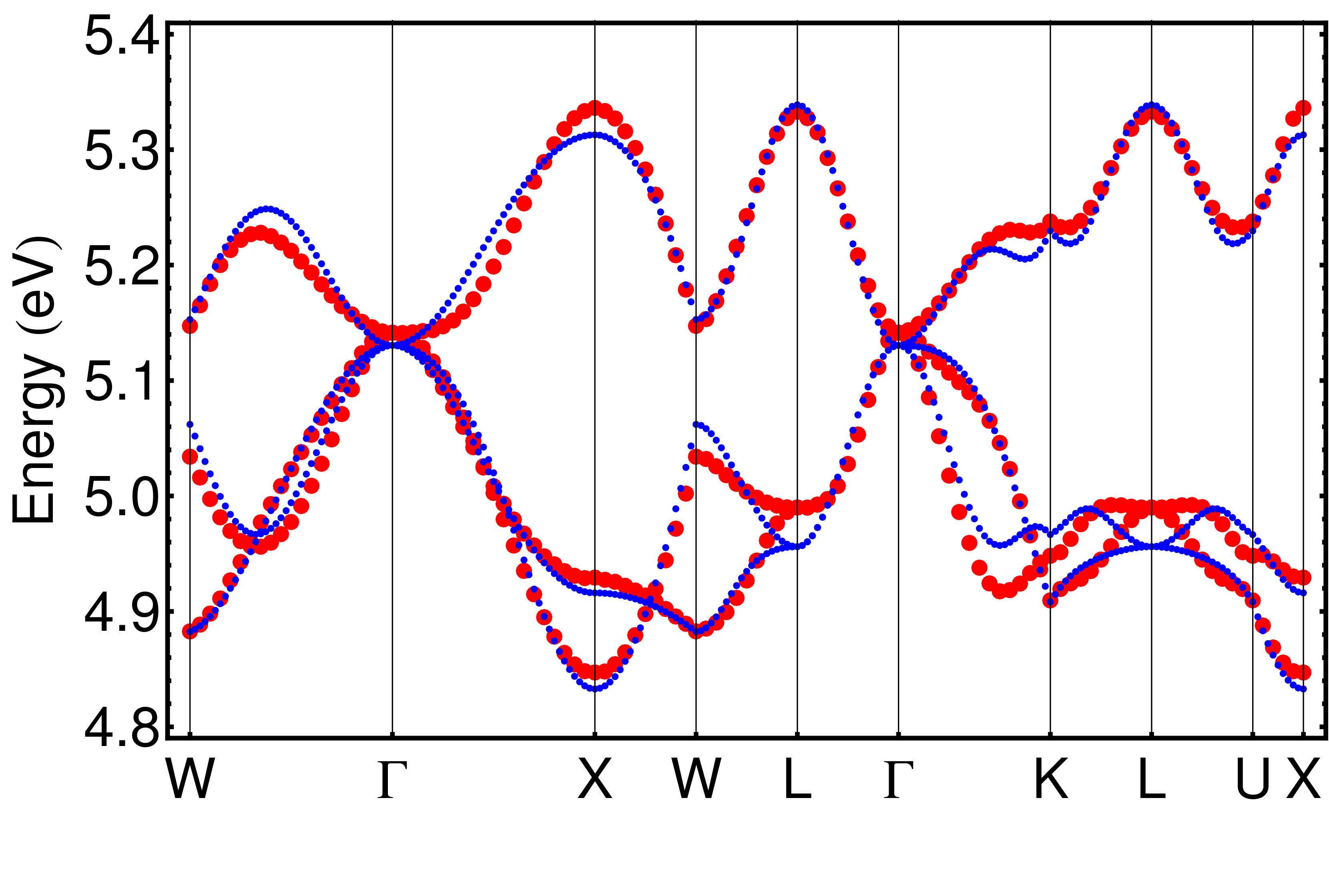
Figure 13: (color online) Band structure of fcc K₃C₆₀ in eV. The red and blue points are obtained from DFT calculations and model Hamiltonian, respectively. The symmetric points $(k_{x},k_{y},k_{z})$ are as follows: $\Gamma=(0,0,0)$, $X=(2\pi/a,0,0)$, $W=(2\pi/a,\pi/a,0)$, $K=(3\pi/2a,3\pi/2a,0)$, $L=(\pi/a,\pi/a,\pi/a)$, $U=(2\pi/a,\pi/2a,\pi/2a)$.

Table 1: LUMO level $\epsilon$ (eV), transfer parameters, and band width $w$ (meV) for K₃C₆₀.

$\epsilon$	$t_{1}$	$t_{2}$	$t_{3}$	$t_{4}$	$t_{5}$	$t_{6}$	$t_{7}$	$w$
5.066	43.3	-31.9	-6.2	-16.6	-9.6	-2.0	2.7	505.9

Appendix B Gutzwiller reduction factors for the LUMO bands and bielectronic energy in $A_{3}$C₆₀

To derive the form of Eq. (20), we apply the Gutzwiller’s approximation extending the one for the nondegenerate band. Vollhardt (1984); Ogawa et al. (1975) Within the Gutzwiller’s approximation, physical quantities are described in terms of the probability $\nu_{\Gamma}$ that one-site electron configuration $\Gamma$ appears in the Gutzwiller’s wave function $|\Psi_{\rm G}\rangle$. Vollhardt (1984); Ogawa et al. (1975)

The occupation number $n_{x}$ in spin orbital $x\sigma$ is described by the probabilities $\nu_{\Gamma}$ as follows:

$$n_{x} = \frac{1}{2}[2\nu_{x}+2\nu_{x\bar{x}}+4\nu_{xy}+4\nu_{zx}$$ (75)

$$+ 4\nu_{xy\bar{x}}+2\nu_{zx\bar{z}}+4\nu_{zx\bar{x}}+2\nu_{xy\bar{y}}+8\nu_{xyz}$$

$$+ 2\nu_{xy\bar{x}\bar{y}}+2\nu_{zx\bar{z}\bar{x}}+8\nu_{xyz\bar{x}}+4\nu_{xyz\bar{y}}+4\nu_{xyz\bar{z}}$$

$$+ 4\nu_{xyz\bar{x}\bar{y}}+2\nu_{xyz\bar{y}\bar{z}}+4\nu_{xyz\bar{z}\bar{x}}+2\nu_{xyz\bar{x}\bar{y}\bar{z}}],$$

where, $1/2$ is due to the spin degrees of freedom, and $\lambda$ and $\bar{\lambda}$ $(\lambda=x,y,z)$ indicate spin orbitals $(\lambda\uparrow)$ and $(\lambda\downarrow)$, respectively. Since we consider the metallic phase, $\nu_{\Gamma}$ does not depend on the spin part of $\Gamma$. For example, $\nu_{x}=\nu_{\bar{x}}$. $n_{y}$ and $n_{z}$ are obtained by cyclic permutation of the indices $(x,y,z)$ in Eq. (75).

The Gutzwiller’s reduction factors $q_{xx}$ appearing in Eq. (21) is given by

$$q_{xx} = \frac{1}{n_{x}(1-n_{x})}\left(\sqrt{\nu_{0}\nu_{x}}+\sqrt{\nu_{\bar{x}}\nu_{x\bar{x}}}+2\sqrt{\nu_{y}\nu_{xy}}\right.$$ (76)

$$+ 2\sqrt{\nu_{z}\nu_{zx}}+2\sqrt{\nu_{y\bar{x}}\nu_{xy\bar{x}}}+\sqrt{\nu_{z\bar{z}}\nu_{zx\bar{z}}}+2\sqrt{\nu_{z\bar{x}}\nu_{zx\bar{x}}}$$

$$+ \sqrt{\nu_{y\bar{y}}\nu_{xy\bar{y}}}+4\sqrt{\nu_{yz}\nu_{xyz}}+\sqrt{\nu_{y\bar{x}\bar{y}}\nu_{xy\bar{x}\bar{y}}}$$

$$+ \sqrt{\nu_{z\bar{z}\bar{x}}\nu_{zx\bar{z}\bar{x}}}+4\sqrt{\nu_{yz\bar{x}}\nu_{xyz\bar{x}}}+2\sqrt{\nu_{yz\bar{y}}\nu_{xyz\bar{y}}}$$

$$+ 2\sqrt{\nu_{yz\bar{z}}\nu_{xyz\bar{z}}}+2\sqrt{\nu_{yz\bar{x}\bar{y}}\nu_{xyz\bar{x}\bar{y}}}+\sqrt{\nu_{yz\bar{y}\bar{z}}\nu_{xyz\bar{y}\bar{z}}}$$

$$+ \left.2\sqrt{\nu_{yz\bar{z}\bar{x}}\nu_{xyz\bar{z}\bar{x}}}+\sqrt{\nu_{yz\bar{x}\bar{y}\bar{z}}\nu_{xyz\bar{x}\bar{y}\bar{z}}}\right)^{2},$$

where $\Gamma=0$ means the configuration with no electron. $q_{yy}$ and $q_{zz}$ are obtained by cyclic permutation of the indices $(x,y,z)$ in Eq. (76). For $q_{\lambda\lambda^{\prime}}(\lambda\neq\lambda^{\prime})$, following relation holds:

$$q_{\lambda\lambda^{\prime}}=\sqrt{q_{\lambda\lambda}q_{\lambda^{\prime}\lambda^{\prime}}}.$$ (77)

The bielectronic energy is

$$E_{\rm bi} = U_{\parallel}(\nu_{x\bar{x}}+\nu_{y\bar{y}}+\nu_{z\bar{z}})$$ (78)

$$+ (U_{\perp}-J_{\rm H}/2)(4\nu_{xy}+4\nu_{yz}+4\nu_{zx})$$

$$+ (3U_{\perp}+J_{\rm H})(2\nu_{xy\bar{x}}+2\nu_{yz\bar{y}}+2\nu_{zx\bar{z}}$$

$$+ 2\nu_{zx\bar{x}}+2\nu_{xy\bar{y}}+2\nu_{yz\bar{z}})$$

$$+ (3U_{\perp}-3J_{\rm H}/2)8\nu_{xyz}$$

$$+ (6U_{\perp}+2J_{\rm H})(\nu_{xy\bar{x}\bar{y}}+\nu_{yz\bar{y}\bar{z}}+\nu_{zx\bar{z}\bar{x}})$$

$$+ (6U_{\perp}-J_{\rm H}/2)(4\nu_{xyz\bar{x}}+4\nu_{xyz\bar{y}}+4\nu_{xyz\bar{z}})$$

$$+ (10U_{\perp})(2\nu_{xyz\bar{x}\bar{y}}+2\nu_{xyz\bar{y}\bar{z}}+2\nu_{xyz\bar{z}\bar{x}})$$

$$+ (15U_{\perp})\nu_{xyz\bar{x}\bar{y}\bar{z}}.$$

The Coulomb contribution (67) to the subband energy level is given by

$$\epsilon_{{\rm bi},x} = \frac{U}{n_{x}}\left[\left(\nu_{x\bar{x}}+2\nu_{xy}+2\nu_{zx}\right)\right.$$ (79)

$$+ 2\left(2\nu_{xy\bar{x}}+2\nu_{zx\bar{x}}+\nu_{xy\bar{y}}+\nu_{zx\bar{z}}+4\nu_{xyz}\right)$$

$$+ 3\left(\nu_{xy\bar{x}\bar{y}}+\nu_{zx\bar{z}\bar{x}}+4\nu_{xyz\bar{x}}+2\nu_{xyz\bar{y}}+2\nu_{xyz\bar{z}}\right)$$

$$+ 4\left(2\nu_{xyz\bar{x}\bar{y}}+2\nu_{xyz\bar{z}\bar{x}}+\nu_{xyz\bar{y}\bar{z}}\right)$$

$$+ \left.5\nu_{xyz\bar{x}\bar{y}\bar{z}}\right].$$

Here, we choose the ordered JT distortion (13). $\epsilon_{{\rm bi},y}$ and $\epsilon_{{\rm bi},z}$ are obtained by cyclic permutation of the indices $(x,y,z)$ in Eq. (79). $\Delta\epsilon_{\rm bi}$ in Eq. (68) is obtained as $\Delta\epsilon_{\rm bi}=\epsilon_{{\rm bi},z}-\epsilon_{{\rm bi},x}$.

References

- Bersuker and Polinger (1989) I. B. Bersuker and V. Z. Polinger, Vibronic Interactions in Molecules and Crystals (Springer–Verlag, Berlin, 1989).
- Bersuker (2006) I. B. Bersuker, The Jahn–Teller Effect (Cambridge University Press, Cambridge, 2006).
- Kaplan and Vekhter (1995) M. D. Kaplan and B. G. Vekhter, Cooperative Phenomena in Jahn-Teller Crystals (Plenum Press, New York and London, 1995).
- Barra et al. (1999) A.-L. Barra, G. Chouteau, A. Stepanov, A. Rougier, and C. Delmas, Eur. Phys. J. B 7, 551 (1999).
- Nakatsuji et al. (2012) S. Nakatsuji, K. Kuga, K. Kimura, R. Satake, N. Katayama, E. Nishibori, H. Sawa, R. Ishii, M. Hagiwara, F. Bridges, T. U. Ito, W. Higemoto, Y. Karaki, M. Halim, A. A. Nugroho, J. A. Rodriguetz-Rivera, M. A. Green, and C. Broholm, Science 336, 559 (2012).
- Krimmel et al. (2005) A. Krimmel, M. Mücksch, V. Tsurkan, M. M. Koza, H. Mutka, and A. Loidl, Phys. Rev. Lett. 94, 237402 (2005).
- Fabrizio and Tosatti (1997) M. Fabrizio and E. Tosatti, Phys. Rev. B 55, 13465 (1997).
- Chibotaru (2005) L. F. Chibotaru, Phys. Rev. Lett. 94, 186405 (2005).
- Chibotaru (2007) L. F. Chibotaru, J. Mol. Struct. 838, 53 (2007).
- Iwahara and Chibotaru (2013) N. Iwahara and L. F. Chibotaru, Phys. Rev. Lett. 111, 056401 (2013).
- Gunnarsson (1997a) O. Gunnarsson, Revs. Mod. Phys. 69, 575 (1997a).
- Ganin et al. (2008) A. Y. Ganin, Y. Takabayashi, Y. Z. Khimyak, S. Margadonna, A. Tamai, M. J. Rosseinsky, and K. Prassides, Nat. Mater. 7, 367 (2008).
- Takabayashi et al. (2009) Y. Takabayashi, A. Y. Ganin, P. Jeglič, D. Arčon, T. Takano, Y. Iwasa, Y. Ohishi, M. Takata, N. Takeshita, K. Prassides, and M. J. Rosseinsky, Science 323, 158 (2009).
- Ganin et al. (2010) A. Y. Ganin, Y. Takabayashi, P. Jeglič, D. Arčon, A. Potočnik, P. J. Baker, Y. Ohishi, M. T. McDonald, M. D. Tzirakis, A. McLennan, G. R. Darling, M. Takata, M. J. Rosseinsky, and K. Prassides, Nature (London) 466, 221 (2010).
- Gunnarsson et al. (1995) O. Gunnarsson, H. Handschuh, P. S. Bechthold, B. Kessler, G. Ganteför, and W. Eberhardt, Phys. Rev. Lett. 74, 1875 (1995).
- Iwahara et al. (2010) N. Iwahara, T. Sato, K. Tanaka, and L. F. Chibotaru, Phys. Rev. B 82, 245409 (2010).
- Stephens et al. (1991) P. W. Stephens, L. Mihaly, P. L. Lee, R. L. Whetten, S.-M. Huand, R. Kaner, F. Deiderich, and K. Holczer, Nature (London) 351, 632 (1991).
- Stephens et al. (1992) P. W. Stephens, L. Mihaly, J. B. Wiley, S.-M. Huand, R. B. Kaner, F. Diederich, R. L. Whetten, and K. Holczer, Phys. Rev. B 45, 543 (1992).
- Gutzwiller (1963) M. C. Gutzwiller, Phys. Rev. Lett. 10, 159 (1963).
- Vollhardt (1984) D. Vollhardt, Revs. Mod. Phys. 56, 99 (1984).
- Lanatà et al. (2012) N. Lanatà, H. U. R. Strand, X. Dai, and B. Hellsing, Phys. Rev. B 85, 035133 (2012).
- Bünemann et al. (1998) J. Bünemann, W. Weber, and F. Gebhard, Phys. Rev. B 57, 6896 (1998).
- Gunnarsson et al. (1996) O. Gunnarsson, E. Koch, and R. M. Martin, Phys. Rev. B 54, R11026 (1996).
- Iwasa and Takenobu (2003) Y. Iwasa and T. Takenobu, J. Phys.: Condens. Matter 15, R495 (2003).
- Chibotaru and Ceulemans (1996) L. F. Chibotaru and A. Ceulemans, Phys. Rev. B 53, 15522 (1996).
- Ceulemans et al. (1997) A. Ceulemans, L. F. Chibotaru, and F. Cimpoesu, Phys. Rev. Lett. 78, 3725 (1997).
- O’Brien (1996) M. C. M. O’Brien, Phys. Rev. B 53, 3775 (1996).
- Auerbach et al. (1994) A. Auerbach, N. Manini, and E. Tosatti, Phys. Rev. B 49, 12998 (1994).
- Gelfand and Lu (1992) M. P. Gelfand and J. P. Lu, Phys. Rev. Lett. 68, 1050 (1992).
- Chibotaru and Ceulemans (2000) L. Chibotaru and A. Ceulemans, AIP Conf. Proc. 544, 19 (2000).
- Nomura et al. (2012) Y. Nomura, K. Nakamura, and R. Arita, Phys. Rev. B 85, 155452 (2012).
- Landau and Lifshitz (1977) L. D. Landau and E. M. Lifshitz, Quantum Mechanics (Non-Relativistic Theory), Third Edition (Butterworth-Heinemann, Oxford, 1977).
- Ogawa et al. (1975) T. Ogawa, K. Kanda, and T. Matsubara, Prog. Theor. Phys. 53, 614 (1975).
- Bünemann et al. (2012) J. Bünemann, F. Gebhard, T. Schickling, and W. Weber, Phys. Status Solidi B 249, 1282 (2012), Sec. 4.1.2.
- Capone et al. (2000) M. Capone, M. Fabrizio, P. Giannozzi, and E. Tosatti, Phys. Rev. B 62, 7619 (2000).
- (36) D. Arčon, private communication.
- Gunnarsson (2004) O. Gunnarsson, Alkali-Doped Fullerides: Narrow-Band Solids with Unusual Properties (World Scientific, Singapore, 2004).
- Lu (1994) J. P. Lu, Phys. Rev. B 49, 5687 (1994).
- Han et al. (1998) J. E. Han, M. Jarrell, and D. L. Cox, Phys. Rev. B 58, R4199 (1998).
- Antropov et al. (1992) V. P. Antropov, O. Gunnarsson, and O. Jepsen, Phys. Rev. B 46, 13647 (1992).
- Landau and Lifshitz (1986) L. D. Landau and E. M. Lifshitz, Theory of Elasticity, Third Edition (Butterworth-Heinemann, Oxford, 1986).
- Shirley and Louie (1993) E. L. Shirley and S. G. Louie, Phys. Rev. Lett. 71, 133 (1993).
- Gunnarsson (1997b) O. Gunnarsson, J. Phys.: Condens. Matter 9, 5635 (1997b).
- Aryasetiawan et al. (2004) F. Aryasetiawan, M. Imada, A. Georges, G. Kotliar, S. Biermann, and A. I. Lichtenstein, Phys. Rev. B 70, 195104 (2004).
- Lof et al. (1992) R. W. Lof, M. A. van Veenendaal, B. Koopmans, H. T. Jonkman, and G. A. Sawatzky, Phys. Rev. Lett. 68, 3924 (1992).
- Chakravarty et al. (1991) S. Chakravarty, M. P. Gelfand, and S. Kivelson, Science 254, 970 (1991).
- Lammert et al. (1995) P. E. Lammert, D. S. Rokhsar, S. Chakravarty, S. Kivelson, and M. I. Salkola, Phys. Rev. Lett. 74, 996 (1995).
- Koch et al. (1999) E. Koch, O. Gunnarsson, and R. M. Martin, Phys. Rev. Lett. 83, 620 (1999).
- Brühwiler et al. (1993) P. A. Brühwiler, A. J. Maxwell, A. Nilsson, N. Mårtensson, and O. Gunnarsson, Phys. Rev. B 48, 18296 (1993).
- Note (1) It was mentioned that Auger spectroscopy mostly probes near-surface layers, Brühwiler et al. (1993) while bulk values of should be reduced by ca eV.
- Note (2) The authors of Ref. \rev@citealpnumBruhwiller1993a disregard the possibility of metallic screening due to the LUMO band and interpret the Auger spectrum of K3C60 on the basis of difference between intra-LUMO () and core ()-LUMO () electron repulsion parameters. However, they did not explain why and should be different in K3C60 and have the same value in pure C60 and K6C60.
- Rosseinsky et al. (1993) M. J. Rosseinsky, D. W. Murphy, R. M. Fleming, and O. Zhou, Nature (London) 364, 425 (1993).
- Ganin et al. (2006) A. Y. Ganin, Y. Takabayashi, C. A. Bridges, Y. Z. Khimyak, S. Margadonna, K. Prassides, and M. J. Rosseinsky, J. Am. Chem. Soc. 128, 14789 (2006).
- Manini et al. (2002) N. Manini, G. E. Santoro, A. Dal Corso, and E. Tosatti, Phys. Rev. B 66, 115107 (2002).
- Note (3) This splitting was identified with the splitting of the LUMO bands at the -point obtained via LDA calculations of NH3K3C60 Manini et al. (2002) and (CH3NH2)K3C60. Potočnik et al. (2012) In both cases the obtained splitting is smaller than the JT splitting of the orbitals in K3C60, which means that LDA calculation do not grasp at all or seriously underestimate the JT effect in these fullerides, which was also the case in other similar calculations. Capone et al. (2000).
- Wehrli et al. (2004) S. Wehrli, T. M. Rice, and M. Sigrist, Phys. Rev. B 70, 233412 (2004).
- Giannozzi et al. (2009) P. Giannozzi et al., J. Phys.: Condens. Matter 21, 395502 (2009).
- Potočnik et al. (2012) A. Potočnik, N. Manini, M. Komelj, E. Tosatti, and D. Arčon, Phys. Rev. B 86, 085109 (2012).