Redshift in a six-dimensional classical Kaluza-Klein type model
Abstract
Multidimensional theories still remain attractive from the point
of view of better understanding fundamental interactions.
In this paper a six-dimensional Kaluza-Klein type
model at the classical, Einstein’s gravity formulation is considered.
The static spherically symmetric solution of
the six-dimensional Einstein equations coupled to the
Klein-Gordon equation with the massless dilatonic field is presented.
As it is horizon free, it is fundamentally different from the four-dimensional Schwarzschild solution. The motion of test particles in such a spherically symmetric configuration is then analyzed. The presence of the dilatonic field has a similar dynamical effect as the
existence of additional massive matter.
The emphasis is put on some observable
quantities like redshifts. It has been suggested that strange features
of emission lines from galactic nuclei as well as quasar-galaxy associations may in fact be manifestations of the
multidimensionality of the world.
Keywords: multidimensional theories, Hamilton-Jacobi equation, redshifts,
quasar-galaxy associations
1 Introduction
And do not be called teachers;
for One is your Teacher,
the Christ Jesus.
Holy Bible, Matthew 23:10
Let the gravitational interaction be described by the Einstein equations [1], [2], [3] and let us suppose that space-time is more than four dimensional [4].
In fact, many 20th century ideas of theoretical physics introduced the possibility that the world may be multidimensional [5].
Among them are the Kaluza-Klein theories
[6] and despite some problems
the continued interest in them also stems from the
fact that the isometry group of the metric
on the extra–dimensional compact internal space
generates gauge symmetries
of the resulting four–dimensional (non-Abelian) gauge
theories [7, 8].
In order that a multidimensional theory,
e.g. a ten-dimensional superstring one,
could be taken as the physically accepted one, it
should possess the proper four-dimensional phenomenology,
primarily the observed bosonic and fermionic fields
spectrum [9].
In this context, new results from the large hadron collider (LHC) experiment are still awaited, including the adjustment of all experimental results [10].
Yet, even if the extra-dimensions effect were noticed
in the LHC experiment, the interpretation of this fact could
possibly possess
the side affect of the (recently increasing) problems,
which lie behind
the experimental validation of the
uncertainty relation (UR) [11].
In that context,
two effects can compete and both of them necessitate a deep theoretical reformulation of UR [12].
The first effect is connected with e.g. i) the
diffraction-interferometric experiments for a photon, where both the uncertainty relation
and the meaning of the half-widths of a pair of functions (time and frequency) related by the Fourier
transform is examined
[13, 14]
and ii) an experiment of the successive projective measurements
of two non-commuting neutron spin components
[15]. In these experiments gravitational effects are not perceived and the
decrease of the right-hand side of the UR, where the Plank constant is, is possibly observed.
The second effect is connected with the space-time curvature impact, which makes the value of the uncertainty of the distance in the coordinate basis bigger than the true one (compare Eq.(43)). These mean that the Plank constant
is in practice multiplied by a constant or functional factor
[11, 16] and in the observation becomes the effective one
[17].
To sum up, the
problems [18], [19]
with the UR and effectiveness of the Plank constant
could be mistakenly taken as the signal
from the extra dimensions in the accelerator experiments.
Meanwhile, there were also attempts in the literature to seek the effects
of the internal space with a small number of extra dimensions (one or two)
in an astrophysical setting.
Previously, these were pursued by Wesson, Lim, Kalligas, Everitt [20]
for one extra dimension and Biesiada, Mańka,
Syska
[21, 22, 23] for two extra dimensions. This line of thinking is worth
developing in order to gain a better understanding of the
possible visibility of manifestations of e.g. the six-dimensionality of the world, not only in the astrophysical observations but, also in
particle experiments [24].
This would mean that the effects of extra dimensions may well be around us [25]
in contrast to standard expectations that extremely high energies are indispensable to probe higher dimensions in search of their existence [26].
The contents of the present paper suggest that there is an
intimate relation between the manifestations of the six-dimensionality
of this world and so-called dark matter (not dark energy). The first conjecture
on the existence of dark matter in galaxies came into play when Oort [27] in 1932
and Zwicky [28] in 1933 applied the famous virial
theorem to the vertical motion of the stars in the Milky Way and to the radial velocities of members of the Coma cluster, respectively, or even
earlier in 1915 when Öpik [29] evaluated the dynamical
density of matter in the Milky Way in the vicinity of the sun. The
problem was revived and became well established in the seventies when
it was demonstrated [30, 31]
that the rotation curves of spiral galaxies were indicative of the possible presence of a
zero luminosity, dark mass, i.e. unseen
in any part of electromagnetic spectrum (except for the visibility of possible
matter which would be its own antimatter). There have been many
suggestions for candidates for dark matter, from the possibly insufficient impact
of massive compact halo objects (MACHOs) [32] such as
“brown dwarfs”, “standard” neutron stars, “nomad planets”
etc. at the one extreme to hypothetical elementary particles like massive neutrinos, axions and other weakly interacting massive particles (WIMPs), which till now are either unable to give the amount of mass needed or are in contradiction with other parts of proposed models [33]. What precisely is dark matter in any detection? Thus, one of the questions is: What, from the scientific point of view, are the inflationary models of all sorts with the persistent lack of observations of their main building blocks, i.e. dark matter and dark energy?
The present paper provides a description of the properties of a certain six-dimensional Kaluza-Klein type model. Section 2 contains a description of the model along with motivations for the choice of six-dimensional space-time (see also [24]). Then, the static spherically symmetric solutions of the multidimensional Einstein equations coupled to the Klein-Gordon equation with the massless dilatonic field [34] are derived [23, 35, 22]. They are in a sense analogous to the familiar four-dimensional Schwarzschild solution but fundamentally different i.e. they are horizon free. A more detailed discussion of the properties of these solutions is presented in Sections 2 and 3. Some strictly observable quantities, such as the redshift formulae, are also briefly discussed. Section 4 is devoted to the analysis of the motion of test particles ruled by the six-dimensional Hamilton-Jacobi equation. The application of the obtained background self-consistent solution [23] in the description of the wave-mechanical structure of e.g. the neutron and its excited states can be found in [24]. Some possible astrophysical and cosmological observational consequences of the model are also presented in Section 4 and in Section 6, which also contains concluding remarks and perspectives. They refer exclusively to relatively tight systems, e.g. the vicinity of a galactic nucleus and a binary galaxy or galaxy-quasar system. The scale invariance of the model is discussed in Section 5. Several more formal, although important, remarks are in the Appendices at the end of this paper. Throughout Section 2 the natural units (c = =1) are used whereas in Sections 3, 4 and 6, which deal with some more observationally oriented issues, the velocity of light is reintroduced explicitly (the Planck constant is irrelevant for this paper considerations).
2 Field equations
The simplest extension of the familiar four-dimensional space-time
models are five-dimensional ones, which were previously considered by
Wesson [20]. In the present paper a six - dimensional model that is more robust
is presented.
The motivations for choosing six-dimensional models by many others were quite diverse. For example, as late as the years 1984-1986, Nishino, Sezgin, Salam and Bergshoeff in
[36] suggested that one can obtain the fermion spectrum by the compactification of the extra two dimensions in a supersymmetric model.
Also, the six-dimensional models of the Kaluza-Klein theory were previously investigated by Ivashchuk and Melnikov [37], Bronnikov and Melnikov [38] and by Mańka and Syska [21].
In [24] the statistical, Fisher
informational reason for the six-dimensionality of space-time was given and
the geometrical properties of the resulting six-dimensional Kaluza-Klein type
model [39],
from the point of view of its impact on the structure of the neutron and its excited states, were also investigated.
The common point of that model [24]
and the one presented below is the basic massless scalar (dilatonic) field obtained simultaneously with the metric tensor field as the self-consistent solution of the coupled Einstein and Klein-Gordon equations. Then, the obtained metric serves as the background for the equation of motion of the new added object, which can be a field [24] or a classical test particle, immersed in the background metric.
The idea of covering the physical structures that are extremely remote in size by one type of mathematical solution is known by the term of scaling in both theoretical and experimental physics [40].
In this respect, both models, the current one and the one presented in [24] possess the same Kaluza-Klein type self-consistent background solution, which formally can be scaled to all distances. More on this can be found in [24] (see also
Section 5).
Yet, whereas in [24] the added object is governed by the Klein-Gordon equation solved (not self-consistently) in the mentioned background metric and the solution is a wave-mechanical one, in the present paper the added object is the classical test particle moving in accordance with the Hamilton-Jacobi equation.
Thus, let us consider a six-dimensional field theory model comprising the gravitational self field described by a metric tensor, ,
and a real massless “basic” scalar field, . This scalar
field is a dilatonic field hence, just below, the minus
sign is present in front of its kinetic energy term
[23, 35].
In a
standard manner we decompose the action into two parts
| (1) |
where is the Einstein–Hilbert action
| (2) |
and is the action for a real massless dilatonic field
| (3) |
In Eqs.(2),(3), denotes the determinant of
the metric tensor, is the curvature scalar of six-dimensional (in general curved) space-time and
denotes the coupling constant of the six-dimensional theory, which is
analogous to the familiar Newtonian gravity constant. is the Lagrangian density for a dilatonic massless
field .
By extremalizing the action given by
Eqs.(1)-(3), we obtain the
Einstein equations
| (4) |
where is the Einstein tensor, is the six-dimensional Ricci tensor and is the energy-momentum tensor of a real dilatonic field , which is given by
| (5) |
Variation of the total action with respect to the field gives the Klein-Gordon equation
| (6) |
where
| (7) |
and is the tensor dual to .
Now, we assume that we live in the compactified (which is quite a reasonable assumption) world, where the six-dimensional space-time is a topological product of “our” curved four-dimensional physical space-time (with the metric ) and the internal space (with the metric ). Therefore, the metric tensor can be factorized as follows
| (8) |
The four-dimensional diagonal part is assumed to be that of a spherically symmetric geometry
| (9) |
where and are (at this stage) two arbitrary functions.
Analogously, we take the two-dimensional internal part to be
| (10) |
The six-dimensional coordinates are denoted by , where is
the usual time coordinate, and are familiar three-dimensional
spherical coordinates in the macroscopic space;
and are coordinates in the internal
two-dimensional parametric space and is
the “radius” of this two-dimensional internal space. We assume
that is the function of the radius in our
external three-dimensional
space [41].
The internal space is a 2-dimensional parametric space with
an -dependent parameter , which can be represented as
a surface embedded in the three-dimensional Euclidean space
| (14) |
Now using Eqs.(9)-(10), we can calculate the components of the Ricci tensor. The nonvanishing components are [23]
| (15) | |||||
| (16) | |||||
| (17) | |||||
| (18) | |||||
Let us assume that we are looking for a solution of the Einstein equations (see Eq.(4)) with the Ricci tensor given by Eqs.(15)-(18), with , and with the following boundary conditions
| (19) |
| (20) |
In other words, we are looking for the solution which at spatial infinity reproduces the flat external four-dimensional Minkowski space-time and static internal parametric space of “radius” , which could be of the order of . However, a much higher value of for the discussed background field configuration, which has, from the point of view of particle physics a very interesting phenomenology, is also possible (compare [24], where for the neutron ).
Now, we make an assumption that the dilatonic field depends neither on time nor on the internal coordinates and . Because of assumed spherical symmetry of the physical space-time, it is natural to suppose that the dilatonic field is the function of the radius alone
| (21) |
We also impose a boundary condition for the dilatonic field
| (22) |
which supplements boundary conditions (19) and
(20) for the metric components.
By virtue of Eqs.(5) and (3), it is easy to see that
the only nonvanishing components of the energy-momentum tensor are
| (23) |
Consequently, it is easy to verify that the solution of the Einstein equations (4) is
| (24) |
| (25) |
| (26) |
Hence, we obtain that the only nonzero component of the Ricci tensor (see Eqs.(15)-(18)) is , which reads
| (27) |
So the curvature scalar is equal to
| (28) |
where is the real constant with the dimensionality of length, whose value is to be taken from observations for each particular system. In the derivation of the above solutions, we have used Eqs.(15)-(18), which together with Eq.(23) imply that all of the six diagonal Einstein equations are equal to just one
| (29) |
Remark: Putting Eqs.(29),(23) and (28) together we can notice a similarity between the equation
| (30) |
and its electromagnetic analog
,
where is the electromagnetic vector potential. Eq.(30)
is the (anti)screening current condition in gravitation that is analogous to
that in electromagnetism or in the
electroweak sector in the self-consistent approach
[22, 42, 43].
Now, we can rewrite the metric tensor in the form
| (31) | |||||
with its determinant equal to
| (32) |
that itself is nonsingular. We see that the space-time of the model is stationary.
It is also necessary to verify whether the solution of the Klein-Gordon equation (6) is in agreement with Eq.(26), which follows from the Einstein equations. According to Eq.(6) and Eqs.(21),(31),(32), we obtain that
| (33) |
where is a constant. Comparing this result with Eq.(26), we conclude that if
| (34) |
then the solution of the Klein-Gordon equation is in agreement with the solution of the Einstein equations coupled to the Klein-Gordon one. Hence, the real massless “basic” dilatonic field given by Eq.(26) can be the source of the nonzero metric tensor given by Eq.(31). Only when the constant is equal to zero do the solutions (24)-(26) become trivial and the six-dimensional space-time is Ricci flat.
It is worth noting that because the components
and of the
Ricci tensor are equal to zero for all values of , the internal
space is always Ricci flat. However, we must not neglect the
internal parametric space because its “radius” is a
function of and the two spaces, external and internal, are
therefore “coupled”. Only when are these two spaces
“decoupled” and our four-dimensional space-time becomes
Minkowski flat.
Remark: When is not equal to zero, our four-dimensional external space-time is curved. Its scalar curvature is equal to (28)
| (35) |
2.1 The stability of the background solution
Let us consider the stability of the self-consistent gravito-dilatonic configuration given by Eqs. (26) and (31). We calculate its energy (see [24]), which is the integral over the spacelike hypersurface [8]
| (36) |
where using Eqs.(23)-(32) we obtain
| (37) |
and
| (38) |
By using the Fisher information formalism, which was developed for the physical models by Frieden and others
[44, 45, 19, 24, 46], the foundation of
the partition of in
Eq.(36) into two parts, was constructed.
The first term, , is connected with the Fisherian kinematical degrees of freedom of
the gravitational configuration and the second one, , is connected with its structural degrees of freedom.
The integrand
in Eq.(38) does not converge on for .
If in Eq.(38), the cutoff is
taken [24], which breaks the self-consistency of the solution,
then it leads to making finite. The value of could be
small in contradistinction to the infinite value obtained in
Eq.(38) for taken in the self-consistent case.
Hence, for , the self-consistent solution given by
Eqs.(26) and (31), which has
energy given by Eq.(37),
cannot be destabilized to yield any other with finite energy.
The energy is the generic property of the solution [47].
In particular, if is a
well-behaved field [48] that depends on
a parameter , then it cannot be destabilized to any
solution with the energy from the sequence that has
the limit ,
which itself corresponds to .
Hence, the transition from the self-consistent gravito-dilatonic
configuration given by Eqs.(26) and
(31) to any others with finite energy
is forbidden [24].
Let us notice that the solution for is consistent with the
Minkowskian space-time one, which has
global energy equal to zero [8].
Therefore, the condition on the right hand side of
Eq.(37) indicates that the
self-consistent gravito-dilatonic configuration
given by Eqs. (26) and (31)
for is more stable than the empty Minkowskian
space-time solution.
Thus, it is worth noting that
this configuration of fields might serve,
under further specific conditions chosen for the particular
physical system
[24], as the background one. It
appears in equations of motions of all new fields that
enter into the system weakly [24].
This suggests that configurations similar to the obtained
self-consistent gravito-dilatonic one could be the main
building materials
for the observed structures in the universe,
both on the microscopic [24] and,
as it is suggested below, on the astrophysical and
cosmological scales, too.
2.2 The problems of the space-time singularity and Kaluza-Klein type excitations
Firstly, in Section 4.2 as far as the space-time geometry is discussed, it will be proven that
the space-time singularity connected with the metric tensor (31) is the one through which only the null geodesics could pass through.
Hence, the obtained solution is not in contradiction with
“cosmic censorship”,
a conjecture that is still not proven
[48].
Secondly, the problem to discuss is the Kaluza-Klein type
excitations. In general, in the Kaluza-Klein gravity, the ground
state solutions can contain a number of the resulting four-dimensional (massless or not) fields [21].
For example, into the presented model, in addition to the six-dimensional dilatonic
field given by Eq.(26), two massless scalars
tied with the shape
of a two-dimensional internal parametric space (14)
could also be incorporated [24].
Then, their existence is
highly constrained by observations that usually tend to
rule out the models. However, this is not the fate of our
non-homogenous solution.
Indeed,
it was noticed in [24] that
unless additional fields enter, on the level of the equations of motion (4) and (6), the theory is scale invariant (see also Section 5).
Yet, when a new scalar field is introduced then the massless dilatonic field of the model, which is the Goldstone one,
gives masses to the “undesirable” Kaluza-Klein type moduli fields.
As the Goldstone mode, the dilatonic field
is absorbed by the new scalar field
introduced into the system [24]. As a result, it was proven that the
obtained ground state solution of the total gravito-dilatonic and
fields configuration
acquires two spinorial degrees of freedom, where the origin of its
non-zero spin
is perceived as a manifestation of both the geometry
of the internal two-dimensional parametric space (14) and of the kinematics of the field inside it. The obtained configuration can be interpreted as, e.g. the neutron
(but other particle solutions are possible also) [24]. Therefore, the model can be extended in such
a way that the intrinsic geometrical and kinematical properties of
fields in the extra dimensions
also manifest themselves in
possible observational consequences in the realm of the
physics of one particle.
In consequence, e.g.
the relevant
observable neutron excited states were also calculated
[24].
To secure the stability of this composite model of the neutron, it was found that the size of the parametric space
has to be equal to [24]. This signifies the large extra dimension solution of ,
which is of the substantial fraction of the nucleon size, which is
evidently not excluded by the experiment [4].
Simultaneously, the inclusion of the additional scalar field
does not lead to the destruction of our background
dilatonic solution (26) as was argued in [24].
Finally, the problem of quantum fluctuations can also be considered. Yet, the existing quantum field theory (QFT)
interpretation of all physical phenomena could and should be
questioned [49]
(see [53, 42, 21]),
i.e. there may
exist physical realities for which the existence of the quantum
fluctuations is not necessary at all. Nowhere is this problem so
crucial as in the case of gravitational interaction, at least
as far as the experiment is considered. If this is a problem of
general relativity, hence, it is also of its Kaluza-Klein gravity
extensions.
In the present paper the astrophysical and cosmological significance of the solution is discussed.
3 Some properties of solutions
If the parameter is strictly positive, then Eqs.(24)-(26) are valid for all . (The discussion of case will be left for A.) The metric tensor becomes singular only at ; nevertheless, its determinant (see Eq.(32)) remains well defined. Below, several formulae which will be useful in the later discussion are collected. We start with time and the radial components of the metric and the internal “radius” (see Eqs.(25) and (31))
| (42) |
It will be also useful to write the explicit relation for the real, physical radial distance from the center
| (43) |
| Example | ||
|---|---|---|
| sun | ||
| globular cluster | ||
| galactic nucleus∗ | ||
| galaxy | ||
| binary galaxy system∗ | ||
| galaxy–quasar system∗ |
Note: Let us recall that in the standard derivation of the Schwarzschild solution, the free parameter in the metric tensor is identified with the total mass of a spherically symmetric configuration due to the demand that at large distances the metric tensor should reproduce the Newtonian potential. Because for (see Eq.(42)), it is interesting to compare the gravitational potential for with the gravitational potential , which is induced by a mass in the Newtonian limit. and are the four-dimensional gravitational constant and the velocity of light, respectively. Comparing these two potentials, we obtain that , so parameter can have similar dynamical consequences as the mass . (The dynamical interpretations of are different for other powers of .) Table 1 contains some astrophysically interesting masses that mimic the values of parameter . In this case, the gravitational potential (see Eq.(31) or Eq.(42)) is attractive although there is no massive matter acting as a source. Nevertheless, we cannot essentially identify parameter directly with . The reason is that the presented solution describes a case where ordinary matter is absent and the (only) contribution to the energy-momentum tensor comes from the infinitely stretched, massless dilatonic field
It is well known [54] that the frequency of light, moving along the geodesic line in a gravitational field that is static or stationary and measured in units of time , is constant () along the geodesic. The frequency of light as a function of the proper time ( ) is equal to
| (44) |
Let us assume that a photon with frequency (measured in units of the proper time ) is emitted from a source that is located at a point where . Then the photon is moving along a geodesic line that reaches the observer () at the point , where , with the frequency
| (45) |
Using Eq.(42) we can rewrite Eq.(45) as
| (46) |
For simplicity, let us consider a limiting case in which the observer is situated at infinity. Then we get
| (47) |
Therefore, we see that the nearer the source is to the center of the field the more the emitted photon is redshifted at the point where it reaches the observer. It should also be emphasized that this redshift does depend on the relative radius rather than separately on and (see also Section 5).
4 Six-dimensional Hamilton-Jacobi equation for a “test particle”
In order to gain a better understanding concerning possible
manifestations of the six-dimensionality of the world, let us
investigate the motion of a “test particle”
of mass
in the central gravitational field described by
Eq.(31). Whether the moving object can be treated as a
“test particle” depends on the value of parameter in the
metric tensor (see Eq.(31)).
The Hamilton-Jacobi equation
| (48) |
describing the motion of a test particle reads
| (49) | |||||
where denotes the complete integral of the Hamilton-Jacobi equation and is the mass of a “test particle” in six-dimensional space-time.
Without loss of generality, we shall restrict ourselves to the motion in the plane , thus
| (50) |
If the integral depends on a non-additive constant, which is the energy (the Hamiltonian does not depend explicitly on time), then the standard procedure of the separation of variables begins with the following factorization of
| (51) |
The separation constants , and have the meaning of the total energy, the effective angular momentum and the internal angular momentum, respectively. Then by separating Eq.(49) into four-dimensional and internal parts, one arrives at the formula
The last equation in (4) is easy to integrate for
| (53) |
where has the meaning of the internal momentum and one can distinguish the square of the (total) internal momentum
| (54) |
Finally, the quantity
| (55) |
in Eq.(4) can be interpreted as the four-dimensional square mass of a test particle in the flat Minkowskian limit at infinity. In the case of the vanishing internal momentum , the four and six-dimensional masses are equal . If the six-dimensional mass is zero , then the four-dimensional mass at spatial infinity would be solely of an internal origin: .
Now, let us consider the radial part , which can easily be read from Eq.(4)
which after formal integration gives
The trajectory of a test particle is implicitly determined by the following equations
| (56) |
| (57) |
where and are constants and without loss
of generality, the initial conditions can be chosen so that
. In other words, integration of
Eq.(57) gives the trajectory of a test
particle and Eq.(56) provides the temporal dependence of
radial coordinate These two relations determine the
trajectory and of a test particle
[55].
Implementing the above outlined procedure, we obtain (from
Eq.(56) and Eq.(4))
| (58) |
and consequently the radial velocity
| (59) |
It is easy to note that the quantity
| (60) |
can be interpreted as the mass in four-dimensional curved space-time. The mass in Eq.(55) is recovered as the limit of for . Similar to our previous discussion, if then and if then the mass would have an internal origin . It should also be emphasized that does depend on the ratio rather than separately on and , which is a reflection of the scale-invariance of the model (see also Section 5 and [24]).
Let us also notice that the non-negativity of the square of the four-dimensional mass gives the first condition on the value of
| (61) |
If the entire spacelike hypersurface is to be accessible for a particle, then from the validity of the condition , the condition follows. Otherwise, Eq.(61) is the condition for the maximum value of the radius
| (62) |
It may appear strange that by which some imaginary values of are also allowed. However,
one should not uncritically transfer
from four-dimensional intuitions (such like
or , although some
of them may turn out to be true) to e.g. the six-dimensional one but rather build on the safe ground
of known properties of four-dimensional sector i.e.
in this case [14].
Now, using the Eq.(57) and Eq.(4) we obtain
| (63) |
and consequently using Eqs.(63) and (59), the angular velocity of the particle reads
| (64) |
Now, the proper angular velocity of the particle is equal to
| (65) |
where is the proper time and
(where is as in Eq.(31)).
The transversal velocity of the particle (i.e. the component perpendicular
to the radial direction) is equal to (see Eq.(43))
| (66) |
and analogously, the transversal component of the proper velocity (written in the units of the proper time ) is equal to
| (67) |
where , and are given
by Eqs.(64),(65) and (43),
respectively.
Let us rewrite Eq.(59) in the following form
| (68) |
where
| (69) |
The function plays the role of effective
potential energy in the meaning that the relation between and determines the allowed regions of
the motion of the particle.
The proper radial velocity of the particle is equal to
| (70) |
where in the last equality the relation is used (see Eq.(42)). So the radial velocity and the proper radial velocity are equal, and one should stress that this property is fundamentally different from the analogous relation for a black hole.
4.1 Stable circular orbits.
Let us consider for a stable circular orbit with given values of , and . The radius of this orbit can be calculated from the following equations (see Eqs.(68), (69),(70))
| (71) |
| (72) |
From Eqs.(72),(68),(69) we obtain the implicit relation between the radius of the stable circular orbit (index ), the angular momentum of the particle and the internal “total momentum”
| (73) |
so
| (74) |
It is easy to verify that because , hence as
tends to infinity.
Using Eqs.(71),(68), (69) we
calculate the total energy of a particle moving along
the stable circular orbit of the radius
| (75) |
or in other words
| (76) |
As the first example, let us consider the motion of a particle with given values of and . Figure 1 illustrates the function for different values of and


Similarly, Figure 2 shows the function for different values of with a fixed value of .
For the particular system is established and is the constant of motion. Yet, there are some physically obvious conditions which in turn restrict admissible values of the radii of stable orbits for a given internal momentum . Namely, from Eq.(73) we obtain
| (77) |
where
| (78) |
and from Eq.(75) we obtain
| (79) |
where
| (80) |
It is easy to verify that condition (77)-(78) is stronger than (79)-(80) which in turn is the one that is stronger than (61), that is
| (81) |
which means that the stability condition of the system is guaranteed by the first inequality in (81), i.e. by the condition (77)-(78). Now, let us calculate the proper angular velocity and the proper transversal velocity of a particle moving along the stable circular orbit determined by Eqs.(71),(72). Using Eqs.(64)-(67) with and given by Eq.(74) and Eq.(76), respectively, we obtain the proper angular velocity
| (82) |
and the proper tangent velocity of the particle
| (83) |
where is given by Eq.(43) for the stable circular orbit. Looking at Eqs.(74),(76), it is not difficult to notice that again depends on the ratio rather than on and independently.
From Eq.(83) and Eqs.(74),(76) and for , one can notice that if
| (84) |
then does not depend explicitly on the mass
of the particle.
However, unless the relation between the proportionality constant and the square of the velocity of light is not unique,
from Eqs.(83),
(74) and (76), it can be noticed that is
additionally parameterized by .
This is clearly the non-classical effect that influences the shape of the rotation curves (Figure 3). The only bounds on that arise in the model follow from the constraints of causality [14] (61), energy (79)-(80) and angular momentum (77)-(78) analyzed above.
For example, the angular momentum constraint (77)-(78)
fulfilled on the entire spacelike hypersurface
gives, according to Eq.(84),
the condition with the lowest bound
on which ,
so that the
internal momentum fulfills the relation .
Although it is not excluded, we do not yet know the rule that forces the proportionality constant in Eq.(84) to be the same for all test particles inside the configuration with the particular central dilatonic field .
Finally, if (phenomenologically) in Eq.(84) is scaled with , then
the profile of the proper tangent velocity given by Eq.(83), and thus the rotation curves, could be modified. The systematic determination of such a rule fulfilled by lies beyond the analysis of this paper.
4.1.1 The case with .
From Eqs.(77)-(78) we notice that if then all values of the radius (or , see Eq.(43)) for stable orbits are allowed. Figure 3 displays the rotation curves calculated according to Eq.(83) (in units of the velocity of light c) for different values of . It shows that the whole effect is i) most pronounced in the region close to the center of the spherically symmetric configuration of the dilatonic field and is, ii) except for the case of discussed below, extended from the center to the infinity. For example, let us take the sun in the Milky Way. Then, e.g. for and at the distance of from the center of the dilatonic field that is overlapping with the center of the Milky Way, we obtain the contribution of (caused by the dilatonic field with the parameter equal to ) to the total proper tangent velocity equal to .

If, however,
| (85) |
then according to Eqs.(77)-(78), the radius of the stable circular orbits has to fulfill the relation
| (86) |
where the limiting value is equal to
| (87) |
In other words, the condition (77)-(78) implies
that one cannot find any stable orbit with
for a fixed ,
which is from the range given by Eq.(85)
and with the angular momentum chosen according to
Eq.(74). In this case, the orbit with is the metastable one. For the limiting value, i.e. for we can notice that .
Note: Above, we have seen that
(for ) is the boundary between configurations of test particles having stable orbits on the entire spacelike hypersurface and configurations with unstable orbits beginning with the radius and upwards. Interestingly, in accordance with Eq.(54), we can also notice that if the value is not to appear in the result of the accidental cancellation, then the square of the internal momentum and the internal angular momentum have to take one of the discrete possibilities, e.g.
| (88) |
respectively, where for the boundary stable configuration.
Yet, this choice also agrees with the axial symmetry of the internal space (14) around
the axis (compare also [24]).
4.1.2 A case with and .
4.2 Radial trajectories, .
In this case, we investigate the free motion of a test particle (with given ) along the geodesic that crosses the center of the gravitational field . Hence, unless it is stated differently, in almost all of Section 4.2. From Eqs.(70) and (68),(69), we obtain
| (89) |
From this we may notice that for a particle which is initially () at rest () at the point , the total energy is equal to (compare Eq.(60))
| (90) |
Therefore, the particle is oscillating and crosses the center with velocity (at the center, the particle becomes massless ). From Eqs.(89), (59) and , we obtain that the acceleration of the particle is equal to
| (91) |
4.2.1 A case with .
From Eq.(91) we see that the acceleration tends to minus infinity at the center and when , it monotonously increases to the zero value when is going to infinity. So, in this case, the particle is attracted to the center for all values of (see Figure 4).


If then from Eq.(91) it follows that with the finite value exists
| (92) |
for which (compare Eq.(87)). In this case, for , the particle is attracted to the center with for and for , the particle is repelled from the center and the acceleration when (see Figure 4). In Figure 5 the radial acceleration of the particle that is very close to the center of the field is presented. Because the solution is horizon free, the achieved values of acceleration of the particle could cause a visible point-like radiation (see Section 6).
4.2.2 A case with and .
4.2.3 The causality condition.
Let us suppose that we have on the entire spacelike hypersurface that is equivalent to the causality condition [14]. Hence, from (61) we see that and from the formula (69), we obtain the condition for the effective potential at infinity, i.e. , with the equality if the limiting value is chosen. With for , which according to (62) is prohibited by the causality condition [14] (61), the potential becomes imaginary.
4.2.4 A case with and .
Now in Eq.(89) we have and from Eqs.(89) and (91), one can read that and for all values of . So, the particle which has both the
six-dimensional mass and the square of the total internal momentum
equal to zero, which is a reasonable
representation of a photon for example, does not feel (except
changing the frequency according to Eq.(44)) the curvature of space-time when moving along the geodesic line crossing the
center.
On the other hand, for ,
and , using Eq.(63)
and introducing formally the
parameter
, we obtain the
trajectory of the particle
| (93) |
When then the trajectory calculated according to the
above equation is a straight line
passing the center at the distance of (impact parameter).
On the other hand, light travelling in our space-time with is deflected even in the absence of baryonic matter (see also
B on the Pericenter shift).
Remark:
We should use the eikonal equation
instead of the Hamilton-Jacobi equation for
and . However, a formal
(technical) substitution of gives the same analytical
result (93).
4.3 Redshift of radiation from stable circular orbits.
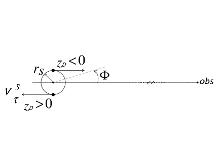
Let us suppose for simplicity’s sake that the observer is located far away from the center of the system at a distance far bigger than the size of the system, so its peculiar motion with respect to the center of the system is negligibly small (see Figure 6). Let us also assume that the dynamical time scale is greater than the characteristic timescale over which the observations are performed i.e. In such a case, the observed motion of the “luminous particle” is seen only as instantaneous redshift or blueshift. If the motion of the “particle”, which is the source, takes place along the stable circular orbit, then the kinematical Doppler shift is equal to (see Figures 6,7)
| (94) |
where the angle (see Eq.(82))
is counted from the direction to observer, i.e.
, as in Figure 6, and the proper tangent velocity is given by Eq.(83).
Now, the gravitational redshift according to Eq.(47) is equal to (see Figure 7)
| (95) |
where .
It is not difficult to see that the combined effect of these redshifts is as follows (see Figure 8)
| (96) |
For a source moving along the stable orbit
away form the observer (which is at infinity), the instantaneous angle is equal to (see Figure 6) and from Eq.(94), we obtain that , i.e. the source is kinematically redshifted and the combined effect given by Eq.(96) obviously has a positive value of the redshift (see the left-hand side of Figure 8).
In the case of the source moving
towards the observer, the instantaneous angle is equal to (see Figure 6) and , i.e. the source is kinematically blushifted. Yet, we notice (see the right-hand side of Figure 8) that for all values of , but small enough values of , even in this case
the combined effect given by Eq.(96) results in a positive value of the redshift . Moreover, for sufficiently small values of
, e.g. for as in Figure 8, even the whole effect of the Doppler blueshift can be hidden behind the gravitational redshift. Because there are no stable orbits for
for (see Eq.(87)), hence for the metastable point
the breaks of the curves (with solid lines) plotted on both the right- and left-hand side of Figure 8 occur.
To summarize, for the square of the total internal
momentum that fulfills relation (85), we obtain
in accordance with Eqs.(86)-(87) that
for all allowed stable radii of the moving source, the possible Doppler blueshift is hidden behind the gravitational redshift caused by the dilatonic central field (see Figure 8).


For small enough values of , the combined Doppler and gravitational effect (96) has a positive value of the redshift for all values of . Yet, for sufficiently small values of , e.g. for , even the whole Doppler blueshift can be hidden behind the gravitational redshift. The breaks of the curves (with solid lines) for are at , as for there are no stable orbits (see Eqs.(86)-(87)).
For example, let us choose as the characteristic value for a system of pairs of galaxies (see 5th row in Table 1). When one of the galaxies in the pair has a four-dimensional mass equal to e.g. and a radius of its stable orbit equal to and , where is the six-dimensional mass of the galaxy, then the value of its total proper tangent velocity that is equal to km/s is obtained. The gravitational redshift (95) of the galaxy is equal to and the maximal value of the Doppler redshift (94) is equal to . Then, the combined effect of the gravitational and Doppler redshifts (see Eq.(96)) is equal to and for a galaxy moving along the stable orbit away from and towards the observer, respectively. Let us notice that, besides the huge value of (the auxiliary mass) connected with the value of the parameter of the gravito-dilatonic configuration (see 5th row in Table 1), the four-dimensional mass of the galaxy forms approximately 70.7% of its six-dimensional mass, which is responsible for the kinematics of the galaxy in its motion around the center of the background gravito-dilatonic field configuration. The remaining 29.3% mass is connected with the galaxy total internal momentum . Thus, in some cases the mass , which enters into the six-dimensional equations of motion could be bigger than the four-dimensional mass , which could be perceived in the four-dimensional space-time.
5 Scale invariance
Let us rewrite the Hamilton-Jacobi equation (see Eq.(49)) in the following way
| (97) | |||||
where
| (98) |
In fact Eq.(97) is scale invariant under
| (99) |
only if this transformation is supplemented by
| (100) |
where is the parameter of the transformation.
Systems with different values of , , , and have the same physical properties provided the values of , , and are the same.
This means that whenever the dilatonic field is present, and unless the symmetry (1)-(3) is broken, the classical picture of the world follows the same patterns from the micro- to the marco-scale only if the complete integral of the system does not change.
Transformation (99) is the symmetry of the action (1)-(3).
This is the invariance of the coupled Einstein
(4) and Klein-Gordon (6) equations, but it
is not the invariance of their solution given by
Eqs.(26) and (31).
This conclusion can also be drawn from Eq.(28).
Hence, we notice that the massless dilatonic
field is the Goldstone field [56].
It would seem that invariance (99) inevitably leads
to the invariance given by Eqs.(99)-(100)
of the Hamilton-Jacobi equation (97).
Yet, the inclusion of any term with mass into the model given
by Eq.(1) will inevitably lead to the
gravitational coupling of this mass
with the metric tensor
part of the Lagrangian, causing the breaking of the original invariance (99).
Hence, the conclusion emerges that there appears a relation between
the four-dimensional mass of the particle and the parameter [24]. This
results from the Einstein equations which fix the value of
after the self-consistent inclusion of the particle
with mass into the configuration of fields. This means that the symmetry connected with the scaling (99) of is broken.
6 Conclusions and perspectives
In this paper the non-trivial, one parametric six-dimensional “background” solution given by Eqs.(31) and (26) with the spherical symmetry in the Minkowski directions of coupled Einstein and Klein-Gordon equations has been presented [23, 22]. It consists in adding to the six dimensional gravity a massless dilatonic field, whose variation in the radial direction compensates self-consistently for the curvature. As a self-consistent [43] and non-iterative one, the solution is also non-perturbative. Here, the dilatonic “basic” field forms a kind of the ground field and the gravitational field (metric tensor) is the self-field [22, 52, 42, 43]. The gravitational component in the four-dimensional space-time is asymptotically flat but fundamentally different from the Schwarzschild solution. Locally, the space-time has the topology of the Minkowki (1,3) 2-dimensional internal space of the varying size, i.e. the six-dimensional world is compactified in a non-homogeneous manner. Next, the motion of a test particle in the six-dimensional space-time of the obtained gravito-dilatonic Kaluza-Klein type model was examined. Additionally, in Section 4.1.1 (see Eq.(88)) it was pointed out that on the stability boundary, the relative internal angular momentum of the particle takes, beginning with zero, all consecutive values with the one half step, i.e. , where .
In Section 2.1 both the problem of the stability of the background
solution and the spectrum of the Kaluza-Klein type excitations were discussed but additional
analysis of the problem can be
found in [24],
where the Fisher-statistical reason for six-dimensionality of the space-time was also discussed.
Nevertheless, since to date we do not see any well-established experimental evidence of the multi-dimensionality of the world [26], hence, from the point of
view of practical purposes, the four-dimensional consistency
alone, which is possessed by a multi-dimensional model, cannot be perceived
as a very important reason for its acceptance.
Therefore, the main physical applicability of the background solution (31),(26) presented in Section 3 refers to its astrophysical and
cosmological signatures for some relatively
tight systems.
Thus, the motion of a test particle in this
background configuration was analyzed. The background solution
is parameterized by the parameter , which (especially for ) has similar dynamical consequences as the mass (see Note below Eq.(43)).
The significance of higher terms in the metric tensor expansion can be different than in e.g. the Schwarzschild solution case (see e.g.
B on the pericenter shift).
Hence, the existence of the self-consistent gravito-dilatonic configuration
(26),(31),
which is perceived by an observer in the same way as invisible
matter, requires taking into account
the nonstandard definition of the system
as one which is both under the self-consistent (Eqs.(6),(4)) and non-self-consistent (Eq.(48)) influence of the gravitational interaction. It was performed
both on the astrophysical (see Section 4) and on the physics of one particle [24] levels.
As the central object does not possess a horizon (as the black-hole does), which is the frequent characteristic of more than four-dimensional solutions [20], thus one of the conclusions from the analysis of this paper is that the visible total redshift-blueshift asymmetry of the radiation from e.g. flows of sources of matter (which consist of test particles) is possible only if they are located sufficiently close to the center of the dilatonic field (Section 4.3). Therefore, the radiation from rotating matter, e.g. around a galaxy center, can originate from an area smaller than that connected with the corresponding Schwarzschild radius (see Note below Eq.(43)) of a black hole. Yet, the observations of predominantly redshifted flows in the presented model can be (see Section 4) explained with special effectiveness for the motion along circular orbits with the internal momentum squared, which fulfills the relation . That is, in this case in the model even the whole Doppler effect connected with the blue wing moving towards us can be hidden below the gravitational redshift effect (see Figures 7,8). Thus, real flows of the matter of some objects can be directed towards us. In fact, all galaxy- and quasar-like objects have to possess proper and four-dimensional square masses (55) in order for them to be observed as redshifted only.
Looking from the above-mentioned perspectives, two classes of phenomena are invoked below.
Firstly,
the statistical analysis performed for the X-ray spectroscopy points to a need for the relativistic effects to be included when modeling the emission from the rotating matter
around the galactic centers [57].
The analysis for the nucleus of the Seyfert
galaxy MCG-06-30-15 [58] was followed by the one for the nuclei of the galaxies MCG-6-30-15, NGC 4593, 3C 120, MCG 6-30-15, MCG 5-23-16, NGC 2992, NGC 4051, NGC 3783, Fairall 9, Ark 120 and 3C 273 [57]. The conclusion was that the relativistic effects, such as the central object spin and the relativistic velocities of flows,
seem to become important in shaping the overall
emission line profile from the inner part of
the rotating matter of accretion disks,
i.e.
from
radii which are probably smaller than .
The characteristics of the observed
emission lines can
correspond to a velocity of
km/s which, in agreement with the analysis in Section 4.1, corresponds to a few values of (see Figure 3).
The observed
lines are asymmetric,
i.e. strong
redshifted emission lines were detected and weaker (or none) blue-shifted ones were seen [59].
Secondly, there are also other phenomena which call for explanations and are hard to understand from the point of view of the standard lore. One class of such problems is connected with the nature of the redshift of galaxies and quasars. It has been known for a long time that the visible associations of quasars and galaxies have been observed where the components have widely discrepant redshifts [60].
We can think of a simple
explanation for such seemingly strange phenomena in terms of the
presented model.
That is, let us imagine that a quasar–galaxy system is captured by the gravito-dilatonic configuration of the field (see 6th row in Table 1).
Supposing that both the quasar and
galaxy are moving along stable orbits,
we
apply the results obtained in Section 4. If the things are so arranged that the quasar (or a group of them) is closer to the center of the background gravito-dilatonic field configuration, then it has a redshift greater than the galaxy located peripherally.
As has been illustrated in Figures 7,8, the smaller the radius of the stable orbit of the quasar is the more significant this effect also is.
Remark: Nevertheless, quasar-like objects are also seen in the vicinity of the central parts of some galaxies. This could be a sign that a galaxy nucleus consists of the background gravito-dilatonic field configuration (see 3rd row in Table 1).
The visibility of bigger values of the redshift of the luminous matter from the inner part of this galaxy nucleus could be blocked by the clumping of the matter orbiting and infalling on it.
Recently a large quasar group (LQG) with 73 members with a huge redshift range was identified in the DR7QSO catalogue of the Sloan Digital Sky Survey [61]. Such a spread of quasars’ redshift can be
understood as resulting from bounding
them in one node of the gravito-dilatonic configuration.
Note: The four-dimensional
part of the metric tensor (9) possesses a
spherical symmetry. Thus, it should be emphasized that in reality the orbits
do not necessarily lay on one plane. Next,
the instantaneous position of an object in space is observed as projected onto a two-dimensional sphere along the light’s geodesics in the curved space-time.
This sphere is then seen as a plane perpendicular to us only. This can obviously place some objects with bigger seemingly closer to the center of the background gravito-dilatonic field configuration. Finally, if constant in Eq.(84) does not have the same value for all orbiting objects then their proper tangent velocities, (83), depend on
and the observational
situation gets more complex.
When the distance from the center is a fraction of ,
the combined gravitational and Doppler redshift given by Eq.(96) becomes the sloping function of thus disclosing the existence of a big redshift discrepancy.
Such a possibility also has an attractive feature that if the quasar–galaxy constitutes a kind of
binary system, then the visible bridge of matter connecting the galaxy and quasar may be explained as a sign of an infall (from the galaxy to the center of the field ) of matter that is passing through the quasar.
Let us also recall that near the center of the field the space-time curvature (28) is large, strongly accelerating (see Eq.(91)) the infalling particles. Therefore, even if the diameter of the quasar size is of AU only then due to the fact that the quasar is located near the center of , does the existence of
the highly nonuniform and anisotropic gravitational field across the quasar interior cause the appearance of large tidal forces inside it. This sheds some light on the nature of the quasar emission as connected with the ultrahigh relative acceleration of particles in its interior, also charged ones, which are mainly electrons. The idea briefly outlined above deserves further, deeper considerations.
Meanwhile,
if a
galaxy was close to the center of the field , let’s say in a stable orbit with (see Figure 4,5), then due to its size it would have been torn into pieces by the tidal forces of the gravito-dilatonic center. This means that the only possibility for a “galaxy” to possess a bigger redshift is to be placed at the center of the background gravito-dilatonic field configuration with the central, highly redshifted opaque inner part of this “galaxy” being
severely overshadowed by the more peripheral luminous matter. This overshadowing
could account for its
faintness.
However, this means that e.g. an object like UDFj-39546284 [62] is not really a “usual” galaxy. Nevertheless, the real obstacle in the precise identification of these objects is the lack of their observed detailed structure.
With
the lack of the confirmation that objects like these emit all wavelengths both shorter than 1.34 and longer than 1.6 , the spectroscopy analysis [62, 63] increases
the doubt about their true galaxy structure .
What is more, there is a great deal of evidence that
redshift is at least partially the intrinsic property of
galaxies and quasars that is apparently quantized
[64, 65, 66, 67, 68].
Its nature is not yet understood
and an analysis of this phenomenon is not covered by the presented, classical model.
The solution to the problem may require
e.g. the modification of the background metric so that the modified one possesses additional minima in the component .
This could be achieved by coupling the Einstein equations (4) to the one which replaces the Klein-Gordon equation (6) and only then solving the Hamilton-Jacobi equation used in this paper for the description of the motion of test particles.
The other possibility for obtaining additional minima of the effective potential could be realized by introducing a new wave function
for a “quasar” system, which fulfills the Klein-Gordon equation (similarly as in [24]), where and are two real field functions. Thus fulfills the equation which is formally similar to the Hamilton-Jacobi
one, (48),
except for the modification of the effective potential caused by a potential of the Bohm’s type (compare [69, 70]). (As Bohm argued, is in this case a general integral and not
the complete one.)
Remark:
The self-consistent gravitational coupling of the matter field
(included into the total fields configuration)
with the metric tensor causes the breaking of the scale invariance of the action (1)-(3), connected with scaling of (see
Section 5).
Thus, due to the Einstein equations, a relation between the four-dimensional mass and the parameter appears whose value is fixed in this way (compare [24]).
An analysis of these two possibilities will be presented in
following papers.
Next, it would be of observational importance to examine e.g. the apparent surface brightness of such sources as galaxies.
Let be the (bolometric) luminosity distance and the angular size distance of a galaxy. Then is the quotient of the total flux received by the observer, which behaves like , to the angular area of the galaxy that is seen by the observer, which goes as , i.e. . Thus, it would be easy to notice that is the function of both the (combined) redshift , (96), and the real distance from the source to the observer.
Remark:
Because
of the integral form (43) of the physical radial distance of the source from the center of the background gravito-dilatonic field configuration, the apparent surface brightness cannot be written
as a simple analytical expression.
Simultaneously, it would also be of interest to examine interactions of the dilatonic-like centers and their distribution in the universe in order to understand its state. The analysis of as the function of and , which depends on , will be discussed in
following papers.
Finally, the observations mentioned above
[71] are still growing in number [72]. These and others [61], like e.g. the helium abundance in the blue hook stars [73], have no
reasonable explanation within the standard interpretation that claims e.g. that
the Hubble expansion is responsible for the redshifts of galaxies or within the theories with the continuous self-creation of matter and the variable mass hypothesis.
There is certainly a need for new models; however, seeking them among the evolutionary ones is not the
proper way.
Acknowledgments
This work has been supported by L.J.Ch..
Thanks to Marek Biesiada for the discussions.
This work has been also supported by the Department of Field
Theory and Particle Physics, Institute of Physics, University of
Silesia.
Appendix A The solution for
If the parameter , then Eqs.(24)-(26) are valid only when . Likewise, in Section 3 we write the temporal and radial components of the metric and the internal “radius” (see Eqs.(25) and (31))
| (104) |
As in Section 2, we have for
(see Eq.(42)). But, comparing
the gravitational potential for with
,
which is the one induced by a mass in the Newtonian limit, we notice that the gravitational potential (see
Eq.(104)) is a repulsive one, contrary to the case for .
The formulae for the scalar curvature (see
Eq.(28)) and dilatonic field Eq.(26) now have the form
| (105) |
| (106) |
where is the constant.
From (104) we see that the metric tensor becomes singular at . However, its determinant (see Eq.(32)) remains well defined. Nevertheless,
we notice that because at the curvature scalar becomes singular and for the field is not defined, hence this metric singularity is a genuine one and a system is well posed only for .
Thus, from Eqs.(105)-(106), it follows that the physical radial distance can be calculated outside the surface only and its value, e.g. from the radius
to the radius , is equal to
| (107) | |||
The region is the only one where a frequency shift can be observed. Using Eq.(104) we can rewrite Eq.(45) as follows
| (108) |
Like before, we take for simplicity’s sake the limit when the observer is in infinity. So we get (see Figure A1)
| (109) |

We obtained the result that the nearer the source was to the surface given by the equation the more the emitted photon which reaches the observer would be blueshifted. This property, caused (in this case) by the repulsive character of the gravitational potential, is the reason why this solution was omitted in the main text, as to date it is rather unnoticed in observations. But, because it formally provides a solution to the model, some of its properties have been reproduced here.
Appendix B Pericenter shift
Let us consider the shift of the point with the minimal , which is the pericenter for a test particle elliptically orbiting a central mass in the spherically symmetric time-independent metric. In Section 3 we pointed out that in the expansion of the metric to the first order in , the parameter has similar dynamical consequences as the mass . The approximate post-Newtonian expression for and of the general metric generated by a central mass can be written as follows [74]
| (110) |
At the lowest order of beyond the Newtonian theory, an orbit undergoes a pericenter shift [74, 75] given by
| (111) |
where is the semi-major axis of the Newtonian ellipse and is the eccentricity ( for an ellipse and for the circle).
The expression (111) is useful for testing different metric theories of gravity with different field equations.
For example if we substitute , corresponding to the general relativity, we get
| (112) |
Now, let us use the formula given by Eq.(111) for the pericenter shift of a test particle orbiting the center of the dilatonic field , (26), with the metric tensor given by Eq.(31) coupled to this field. Neglecting the influence of the internal two-dimensional space (which is reasonable for ) and expanding and given by Eq.(31) to the second and first order in , respectively, we obtain
| (113) |
Comparing (113) with the approximate post-Newtonian result (B), for we get the following approximate values of the post-Newtonian parameters in our model
| (114) |
Hence, from Eq.(111) we finally obtain
| (115) |
Thus, e.g. for a test particle on the orbit with the radius , where (see Table 1 for values of ), the pericenter shift is equal to and for and , respectively. In the post-Newtonian approximation used, the negative sign is characteristic for the influence of the dilatonic field which leads to a retrograde pericenter shift.
References
References
- [1] C.W.F. Everitt et al., Gravity Probe B: Final Results of a Space Experiment to Test General Relativity, Phys.Rev.Lett. 106, 221101, doi:10.1103/PhysRevLett.106.221101, (2011). J. Beringer et al.(PDG), Chapter 20 on Experimental tests of gravitational theory, T. Damour, (October 2011), PR D 86, 010001, (2012), http://pdg.lbl.gov.
- [2] The analysis could be performed in accordance with an effective gravity theory of the Logunov type [3] with, of course, somehow different consequences.
- [3] V.I. Denisov and A.A. Logunov, The Theory of Space-Time and Gravitation, in Gravitation and Elementary Particle Physics, Physics Series, ed. A.A. Logunov, (MIR Publishers, Moscow), 14-130, (1983). C. Lämmerzahl, Testing Basic Laws of Gravitation Are Our Postulates on Dynamics and Gravitation Supported by Experimental Evidence? in Mass and Motion in General Relativity, Editors: L. Blanchet, A. Spallicci, B .Whiting, (Springer), 25-65, (2011). G. F. R. Ellis, Note on Varying Speed of Light Cosmologies, General Relativity and Gravitation 39 (4), 511 520, (2007), arXiv:astro-ph/0703751v1.
- [4] I. Bars, J. Terning, F. Nekoogar (Founding Ed.), Extra Dimensions in Space and Time, (Springer), (2010). J. Beringer et al., (Particle Data Group), J. Parsons, A. Pomarol, Chapter on Extra Dimensions, 4-5, (November 2011), PR D 86, 010001, URL:http://pdg.lbl.gov, (2012).
- [5] M.B. Green and J.H. Schwarz, Supersymmetrical dual string theory, Nucl. Phys. B 181, 502-530, (1981). M.B. Green and J.H. Schwarz, Supersymmetric dual string theory III, Nucl.Phys.B 198, 441, (1982). M. Kaku, Introduction to Superstrings, (Springer, New York), (1988).
- [6] R. Kerner, Generalization of the Kaluza-Klein theory for an arbitrary non-abelian gauge group, Ann.Inst. H. Poincaré, Vol.IX, no.2, 143-152, (1968).
- [7] D. Bailin, A. Love, Kaluza-Klein theories, Rep.Prog.Phys. 50, 1087-1170, (1987).
- [8] Y. Choquet-Bruhat, General Relativity and Einstein s Equations, pp.653-662,742, (Oxford Univ. Press), (2009).
- [9] M.B. Green, J.H. Schwarz, E. Witten, Superstring theory, Vol.2, Loop amplitudes, anomalies phenomenology, (Cambridge Univ. Press), (1988). W.-Z. Feng, D. Lüst, O. Schlotterer, Nucl.Phys. B 861, 175-235, doi:10.1016/j.nuclphysb.2012.03.010, (2012).
- [10] The BABAR Collaboration, Evidence for an excess of decays, SLAC-PUB-15028, arXiv:1205.5442v1, 24 May 2012.
-
[11]
J.Y. Bang, M.S. Berger, Quantum mechanics and
the generalized uncertainty principle,
Phys.Rev.D 74, pp.125012:1-8,
doi:10.1103/PhysRevD.74.125012, (2006).
Ben-Rong Mu, Hou-Wen Wu, Hai-Tang Yang, Generalized Uncertainty Principle in the Presence of Extra Dimensions, Chin.Phys.Lett. Vol.28(9), 091101, doi:10.1088/0256-307X/28/9/091101, (2011). - [12] M. Ozawa, Universal Uncertainty Principle, Simultaneous Measurability, and Weak Values, (QCMC): The Tenth International Conference 2010, AIP Conf. Proc. 1363, 53-62, doi:http://dx.doi.org/10.1063/1.3630147, (2011), arXiv:1106.5083v2.
- [13] The nature of light. What is a photon?, pp.372,374, Edited by Ch. Roychoudhuri, A.F. Kracklauer, K. Creath, (CRC Press, Taylor&Francis Group), (2008).
- [14] J. Sładkowski, J. Syska, Information channel capacity in the field theory estimation, Phys.Lett.A 377 18-26, doi:10.1016/j.physleta.2012.11.002, (2012), arXiv:1212.6105.
- [15] J. Erhart, S. Sponar, G. Sulyok, G. Badurek, M. Ozawa and Y. Hasegawa, Experimental demonstration of a universally valid error disturbance uncertainty relation in spin measurements, Nature Physics 8, 185 189, doi:10.1038/nphys2194, (2012).
- [16] C. Roychoudhuri, Foundations of Physics 8 (11/12), 845 (1978). J. Syska, Has Quantum Field Theory the Standard Transition from Poisson Brackets?, Int.J. of Theoretical Phys., Vol.42, No.5, 1085-1088, (2003).
- [17] M. Spanner, I. Franco and P. Brumer, Coherent control in the classical limit: Symmetry breaking in an optical lattice, Phys.Rev.A 80, 053402, doi:10.1103/PhysRevA.80.053402, (2009). A. Matzkin, Entanglement in the classical limit: Quantum correlations from classical probabilities, Phys.Rev.A 84, 022111, doi:10.1103/PhysRevA.84.022111, (2011).
- [18] As a consequence the UR loses its contact with the observational results and has to be abandoned on behalf of the multiparametric Rao-Cramér inequality, as not only the operational but the more fundamental one [19, 14].
- [19] J. Syska, Maximum likelihood method and Fisher’s information in physics and econophysics, (polish version), University of Silesia, arXiv:1211.3674 [physics.gen-ph], http://el.us.edu.pl/ekonofizyka/images/f/f2/Fisher.pdf , (2011).
- [20] P.S. Wesson, A physical interpretation of Kaluza-Klein cosmology, Ap.J 394, 19, (1992). P. Lim, J.M. Overduin and P.S. Wesson, J. Math. Phys. 36, 6907, (1995). D. Kalligas, P.S. Wesson, and C. W. F. Everitt, The Classical tests in Kaluza-Klein gravity, Ap.J, Part 1, vol. 439, no.2, 548 557, (1994).
-
[21]
R. Mańka and J. Syska, Torus compactification of
six-dimensional gauge theory, J.Phys.G: Nucl.Part.Phys. 15, 751-764, (1989).
J. Syska, Remarks on self-consistent models of a particle, Trends in Boson Research, e.d. A.V. Ling, (Nova Science Publishers), 163-181, (2006). - [22] J. Syska, Self-consistent classical fields in field theories, PhD thesis (unpublished), (University of Silesia), (1995/99).
- [23] M. Biesiada, R. Mańka and J. Syska, A new static spherically symmetric solution in six-dimensional dilatonic Kaluza-Klein theory, Inter.Journal of Modern Physics D, Vol.9, Nu.1, 71-78, (2000); R. Mańka and J. Syska, Nonhomogeneous six-dimensional Kaluza-Klein compactification, preprint UŚL-TP-95/03, (University of Silesia), (1995).
- [24] J. Syska, Kaluza-Klein Type Model for the Structure of the Neutral Particle-like Solutions, Int.J.Theor.Phys., Vol.49, Issue 9, 2131-2157, doi:10.1007/s10773-010-0400-8, Open Access, (2010).
- [25] G. Bertone, G. Servant and G. Sigl, Indirect detection of Kaluza-Klein dark matter, Phys.Rev. D 68, 044008, (2003). A.F. Zakharov, F. De Paolis, G. Ingrosso, A.A. Nucita, Shadows as a tool to evaluate black hole parameters and a dimension of spacetime, New Astronomy Reviews, Vol.56, Issues 2 3, 64 73, (2012).
- [26] S. Chatrchyan et al. (CMS Collaboration), Search for Signatures of Extra Dimensions in the Diphoton Mass Spectrum at the Large Hadron Collider, PRL 108, 111801, (2012).
- [27] J.H. Oort, The force exerted by the stellar system in the direction perpendicular to the galactic plane and some related problems, Bull.Astr.Inst. Netherlands VI, 249-287, (1932).
- [28] F. Zwicky, Die Rotverschiebung von extragalaktischen Nebeln, Helv.Phys.Acta 6, 110-127, (1933).
- [29] E. Öpik, Bull. de la Soc. Astr. de Russie 21, 150,(1915).
- [30] V.C. Rubin and W.K. Ford, Ap.J 379, (1970). V.C. Rubin, W.K. Ford, and N. Thonnard, Rotational Properties of 21 Sc galaxies with a large range of luminosities and radii. From NGC 4605 ( kpc) to UGC 2885 ( kpc), Ap.J 238, 471, (1980).
- [31] E.I. Gates, G. Gyuk, and M.S. Turner, Microlensing and Halo Cold Dark Matter, Phys.Rev.Lett. 74, 3724-3727, (1995). E.I. Gates, G. Gyuk and M.S. Turner, The Local Halo Density, Ap.J.Lett., 449, L123 L126, (1995).
- [32] P. Tisserand et al., Limits on the Macho content of the Galactic Halo from the EROS-2 Survey of the Magellanic Clouds, 387-404, A&A 469, doi: 10.1051/0004-6361:20066017, (2007). L. Wyrzykowski, J. Skowron, S. Kozłowski, A. Udalski, M.K. Szymański, M. Kubiak, G. Pietrzyński, I. Soszyński, O. Szewczyk, K. Ulaczyk, R. Poleski and P. Tisserand, The OGLE view of microlensing towards the Magellanic Clouds IV. OGLE-III SMC data and final conclusions on MACHOs, Mon.Not.R.Astron.Soc., 416, 2949 2961, doi: 10.1111/j.1365-2966.2011.19243.x, (2011). S. Calchi Novati, Microlensing towards the Magellanic Clouds and M31: is the quest for MACHOs still open?, J.Phys.: Conf.Ser. 354, 012001, doi:10.1088/1742-6596/354/1/012001, (2012).
- [33] The Review of Particle Physics, K. Nakamura et al. (Particle Data Group), Chapter 22, 1-19, Dark matter, Revised September 2011 by M. Drees (Bonn University) and G. Gerbier (Saclay, CEA), J.Phys.G 37, 075021 (2010) and 2011 partial update for the 2012 edition. M.J. Disney, J.D. Romano, D.A. Garcia Appadoo, A.A. West, J.J. Dalcanton and L. Cortese, Galaxies appear simpler than expected, Nature 455, 1082-1084, doi:10.1038/nature07366, (23 October 2008). R.H. Sanders, Modified Newtonian Dynamics: A Falsification of Cold Dark Matter, Advances in Astronomy, Volume 2009, (2009), Article ID 752439, doi:10.1155/2009/752439. P. Kroupa, The dark matter crisis: falsification of the current standard model of cosmology, (2012), arXiv:1204.2546v1. P. Kroupa, B. Famaey, K.S. de Boer, J. Dabringhausen, M.S. Pawlowski, C.M. Boily, H. Jerjen, D. Forbes, G. Hensler, and M. Metz, Local-Group tests of dark-matter concordance cosmology. Towards a new paradigm for structure formation, (2010), arXiv:1006.1647v3.
-
[34]
This
dilatonic field is the created
fluctuation out from nothingness (my footnote).
P. Forgács, J. Gyürüsi, Static spherically symmetric monopole solutions in the presence of a dilaton field, Phys.Lett.B 366, pp.205-211, doi:10.1016/0370-2693(95)01321-0, (1996), arXiv:hep-th/9508114v2.
G. Chechelashvili, G. Jorjadze, Dilaton Field and Massless Particle for 2d Gravity, Workshop ISPM-98, Tbilisi September 12-18, (1999), arXiv:hep-th/9908206. - [35] M. Biesiada, K. Rudnicki and J. Syska, An alternative picture of the structure of galaxies, in Gravitation, Electromagnetism and Cosmlogy: toward a new synthesis, ed. K. Rudnicki, (Apeiron, Montreal), 31-47, (2001).
- [36] M. Nishino and E. Sezgin, Matter and gauge couplings of N = 2 supergravity in six dimensions, Phys. Lett. B 144, 187-192, (1984). E. Bergshoeff, A. Salam and E. Sezgin, A supersymetric -action in six dimensions and torsion, Phys.Lett.B 173, 73-76, (1986). A. Salam and E. Sezgin, Chiral compactification on Minkowski of N=2 Einstein-Maxwell supergravity in six dimensions, Phys.Lett. B 147, 47, (1984).
- [37] V.D. Ivashchuk and V.N. Melnikov, Class.Quantum Grav. 11, 1793, (1994). V.D. Ivashchuk and V.N. Melnikov, Grav. & Cosmol. 1 No2, 133, (1995); V.D. Ivashchuk, PhD Dissertation, (VNICPV, Moscow), (1989).
- [38] K.A. Bronnikov and V.N. Melnikov, Annals of Physics (N.Y.) 239, 40, (1995).
- [39] The dimension of the resulting space-time for the multi-dimensional field theory model depends on the number of degrees of freedom of the field in our four-dimensional Minkowski space-time [24, 44]. For example, in the case of electromagnetism for which , the arising space-time is eight-dimensional. The obtained field theory model is called the Kaluza-Klein type model.
- [40] G.I. Barenblatt, Scaling, (Cambridge Univ. Press), (2003).
- [41] Thanks to Ryszard Mańka for pointing in this direction.
- [42] J. Syska, Boson ground state fields in the classical counterpart of the electroweak theory with non-zero charge densities, in Frontiers in field theory, ed. O. Kovras, (Nova Science Publishers), (New York 2005), chapter 6, 125-154 and in Focus on Boson Research, (Nova Publishers), 233-258, (2006), arXiv:hep-ph/0205313.
- [43] J. Syska, The weak bound state with the non-zero weak charge density as the LHC 126.5 GeV state, paper in the review, (2013), arXiv:1305.1237 [hep-ph].
- [44] B.R. Frieden, A probability law for the fundamental constants, Found.Phys., Vol.16, No.9, 883-903, (1986). B.R. Frieden, Fisher information, disorder, and the equilibrium distributions of physics, Phys.Rev.A 41, 4265-4276, (1990). B.R. Frieden, B.H. Soffer, Lagrangians of physics and the game of Fisher-information transfer, Phys.Rev.E 52, 2274-2286, (1995). B.R. Frieden, Relations between parameters of a decoherent system and Fisher information, Phys.Rev.A 66, 022107, (2002). B.R. Frieden, A. Plastino, A.R. Plastino and B.H. Soffer, Schrödinger link between nonequilibrium thermodynamics and Fisher information, Phys.Rev.E 66, 046128, (2002). B.R. Frieden, A. Plastino, A.R. Plastino and B.H. Soffer, Non-equilibrium thermodynamics and Fisher information: An illustrative example, Phys.Lett.A 304, 73-78, (2002). B.R. Frieden, Science from Fisher information: A unification, (Cambridge Univ. Press), (2004).
-
[45]
J. Syska, Fisher information and quantum-classical field
theory: classical statistics similarity, Phys. Stat. Sol.(b) 244, No.7, 2531-2537, (2007)/DOI 10.1002/pssb.200674646,
arXiv:physics/0811.3600.
E.W. Piotrowski, J. Sładkowski, J. Syska, S. Zaja̧c, The method of the likelihood and the Fisher information in the construction of physical models, Phys. Stat. Sol.(b), 246, No.5, 1033-1037, (2009)/DOI 10.1002/pssb.200881566, arXiv:physics/0811.3554. - [46] J. Syska, Frieden wave-function representations via an Einstein-Podolsky-Rosen-Bohm experiment, Phys.Rev.E. 88, No.3, 032130, doi:10.1103/PhysRevE.88.032130, (2013).
-
[47]
M. Peixoto,
Structural stability on two-dimensional manifolds,
Topology 1, Issue 2, 101 120, (1962).
M. Brin, G. Stuck, Introduction to dynamical systems, (Cambridge Univ. Press), (2003). - [48] A.D. Rendall, Partial differential equations in general relativity, pp.19,180-184, (Oxford Univ. Press), (2008).
- [49] Because of this, e.g. quantum chromodynamics (QCD) is a theory without final fundamental success, as was expressed in [50]: “… all spin parts have to add to which is incredible in the light of the present day experiments. This may indicate that some underlying symmetries, unknown at present, are playing a role in forming the various contributing parts such that the final sum rule gives the fermion value”. In this respect the theoretical situation of QCD (which by composing nucleon from point-like “partons” has recently proposed a kind of a “planetarian” approach) has not improved at all [51]. Its problem, contrary to the self-consistent approach [22, 52, 42, 43], consists in an attempt to regain the classical non-zero extended charge density that was quantized earlier.
- [50] K. Heyde, Basic ideas and concepts in nuclear physics, 3rd ed., IOP Publishing Ltd, p.577, (2004).
- [51] F. Gross, G. Ramalho and M.T. Peña, (2012), arXiv:1201.6337v1 .
- [52] R. Mańka and J. Syska, Phys.Rev.D 49, Nu.3, pp.1468-78, (1994). This paper is drastically reinterpreted by [42] and [43].
- [53] B.O. Barut, J. Kraus, Nonperturbative quantum electrodynamics: The Lamb shift, Found.Phys. 13, 189-194, doi:10.1007/BF01889480, (1983). A.O. Barut, J.F. Van Huele, Quantum electrodynamics based on self-energy: Lamb shift and spontaneous emission without field quantization, Phys.Rev.A 32, 3187-3195, doi:10.1103/PhysRevA.32.3187 , (1985). A.O. Barut, J.P. Dowling, Quantum electrodynamics based on self-energy: Spontaneous emission in cavities, Phys.Rev.A 36, 649-654, doi:10.1103/PhysRevA.36.649 , (1987). A.O. Barut, Combining relativity and quantum mechanics: Schrödinger’s interpretation of , Found.Phys. 18, 95-105, doi:10.1007/BF01882875, (1988); Schrödinger’s interpretation of psi as a continuous charge distribution, Ann.Phys. (Leipzig), 45, 31-36, (1988); The revival of Schrödinger’s interpretation of quantum mechanics, Found.Phys.Lett. 1, 47-56, doi:10.1007/BF00661316, (1988). A.O. Barut, Quantum-electrodynamics based on self-energy, Phys.Scr. T 21, 18-21, (1988); A.O. Barut, Y.I. Salamin, Relativistic theory of spontaneous emission, Phys.Rev.A 37, 2284-2296, doi:10.1103/PhysRevA.37.2284 (1988). A.O. Barut and N. Ünal, An exactly soluble relativistic quantum two-fermion problem, J.Math.Physics 27, 3055, doi:10.1063/1.527235, (1986); A.O. Barut and N. Ünal, Physica A 142, A new approach to bound-state quantum electrodynamics: I. Theory, 467-487, doi:10.1016/0378-4371(87)90036-7, and A new approach to bound-state quantum electrodynamics: II. Spectra of positronium, muonium and hydrogen, 488-497, doi:10.1016/0378-4371(87)90037-9, (1987).
- [54] L.D. Landau and E.M. Lifshitz, The classical Theory of Fields, (Pergamon Press, New York), (1975). V. Petkov, On the gravitational redshift, (2001), arXiv:gr-qc/9810030; Propagation of light in non-inertial reference frames, (2003), arXiv:gr-qc/9909081v7.
- [55] W. Rubinowicz and W. Królikowski, Mechanika teoretyczna, (Polish Scientific Publishers, Warszawa), (1980). E.T. Whittaker, A Treatise on the Analytical Dynamics of Particles and Rigid Bodies, (Cambridge Univ. Press, London), (1904).
- [56] M.B. Green, J.H. Schwarz, E. Witten, Superstring theory, Vol.2, chapter 13, (Cambridge Univ. Press), (1988).
-
[57]
L.W. Brenneman and Ch.S. Reynolds, Relativistic broadening of iron emission lines in a sample of active galactic nuclei,
Ap.J 702, No.2, 1367-1386,
doi:10.1088/0004-637X/702/2/1367, (2009).
M. Guainazzi, S. Bianchi, M. Dove iak, Statistics of relativistically broadened Fe K lines in AGN, Astron.Nachr., Vol.327, Issue 10, 1032, (2006). - [58] L.W. Brenneman and Ch.S. Reynolds, Constraining black hole spin via X-ray spectroscopy, Ap.J, 652, 1028-1043, (2006).
- [59] Y. Tanaka, K. Nandra, A.C. Fabian, H. Inoue, C. Otani, T. Dotani, K. Hayashida, K. Iwasawa, T. Kii, H. Kunieda, F. Makino, M. Matsuoka, Gravitationally redshifted emission implying an accretion disk and massive black hole in the active galaxy MCG 6 30 15, Nature 375, 659-661, (1995). M. Guainazzi, et al., A&A 341, L27, (1999). K. Iwasawa, et al., MNRAS 282, 1038, (1996). M. Guainazzi, et al., A&A 341, L27, (1999). J.C. Lee, A.C. Fabian, W.N. Brandt, C.S. Reynolds, & K. Iwasawa, MNRAS 310, 973, (1999). J.C. Lee, A.C. Fabian, C.S. Reynolds, W.N. Brandt, & K. Iwasawa, MNRAS 318, 857, (2000). J.C. Lee, K. Iwasawa, J.C. Houck, A.C. Fabian, H.L. Marshall, & C.R. Canizares, ApJ 570, L47, (2002). A.J. Young, J.C. Lee, A.C. Fabian, C.S. Reynolds, R.R. Gibson, & C.R. Canizares, ApJ 631, 733, (2005). J. Wilms, C.S. Reynolds, M.C. Begelman, J. Reeves, S. Molendi, R. Staubert, & E. Kendziorra, MNRAS 328, L27, (2001). A.C. Fabian, et al., MNRAS 335, L1, (2002). C.S. Reynolds, J. Wilms, M.C. Begelman, R. Staubert, & E. Kendziorra, MNRAS 349, 1153, (2004).
- [60] H. Arp, E. Giraud, J.W. Sulentic and J.P. Vigier, Pairs of spiral galaxies with magnitude differences greater than one, A&A 121, No.1, 26-28, (1983).
- [61] R.G. Clowes, K.A. Harris, S. Raghunathan, L.E. Campusano, I.K. Söchting, M.J. Graham, A structure in the early Universe at that exceeds the homogeneity scale of the R-W concordance cosmology, MNRAS 429, pp.2910-2916, doi:10.1093/mnras/sts497, (2013).
- [62] R.J. Bouwens, G.D. Illingworth and the HUDF09 Team, Supplementary Information for Nature Letter Searches and limits for z 10 galaxies in the HST HUDF09 Data, Supplementary Information for Nature Letter, doi: 10.1038/nature09717, (2011).
- [63] G.P. Smith, D.J. Sand, E. Egami, D. Stern and P.R. Eisenhardt, Optical and Infrared Nondetection of the z = 10 Galaxy behind Abell 1835, Ap.J, 636, 575-581, (2006).
- [64] H. Arp, A corrected velocity for the local standard of rest by fitting to the mean redshift of local group galaxies, A&A 156, No.1-2, 207-212, (1986).
- [65] W.G. Tifft, in New Ideas in Astronomy, eds. F. Bertola, J. Sulentic and B. Madore, (Cambridge Univ. Press), 173, (1988).
- [66] W.G. Tifft, Preprint of Steward Observatory No.1143, (1993). W.G. Tifft, Redshift quantization - a review, Astrophysics and Space Science, Vol.227, No.1-2/May, 25-39, (1995). W.G. Tifft, Global redshift periodicities and variability, ApJ 485, Nu.2, 465-483, (1997).
- [67] L. Anderson, E. Aubourg, S. Bailey, et al., The clustering of galaxies in the SDSS-III Baryon Oscillation Spectroscopic Survey: baryon acoustic oscillations in the Data Release 9 spectroscopic galaxy sample, Mon.Not.Roy.Astron.Soc. 427, Issue 4, 3435-3467, (2013), arXiv:1203.6594. C.C. Fulton and H.C. Arp, The 2df redshift survey. I. Physical association and periodicity in quasar families, Ap.J, 754, 134, (10pp), (2012), doi:10.1088/0004-637X/754/2/134.
- [68] P.M. Hansen, Astronomical redshifts of highly ionized regions, Astrophys Space Sci 352, 235 244, (2014), doi:10.1007/s10509-014-1910-2.
- [69] O. Davis Johns, Analytical Mechanics for Relativity and Quantum Mechanics, pp.483-485, (Oxford Univ. Press), (2005).
- [70] D. Bohm, Phys.Rev. 85, pp.166 and 180, (1952). D. Bohm, Phys.Rev. 87, 389, (1952).
- [71] G. Burbidge and M. Burbidge, Quasi-Stellar Objects, (Freeman, San Francisco, 1967). H. Arp, E. Giraud, J.W. Sulentic and J.P. Vigier, A&A 121, No.1, 1,26 (1983). H. Arp, Quasars, redshifts and controversies, (Interstellar Media, Berkeley), (1987). Zhu Xing-fen and Chu Yao-quan, Periodic redshift distribution of quasars associated with low redshift galaxies, Chinese Astronomy and Astrophysics Vol.14, Issue 4, 429-436, (December 1990). G. Burbidge and A. Hewitt, Sky and Telescope, 32, (December 1994). Gong Shu-mo and Xia Chang-li, Statistical analysis of emission and absorption lines of quasars. II. An analysis of 6761 , Chinese Astronomy and Astrophysics Vol.23, Issue 1, 17-21, (January-March 1999). H. Arp, Arguments for a Hubble Constant near H0 = 55, Ap.J 571, 615 618, (2002). G. Burbidge, E.M. Burbidge and H. Arp, The nature of the ultraluminous X-ray sources inside galaxies and their relation to local QSOs, A&A 400, L17-L19 (2003), astro-ph/0211139. E.M. Burbidge & G. Burbidge, The Ejection of QSOs from AGN: A Phenomenon that Cannot be Denied, in Suzy Collin, Fran oise Combes and Isaac Shlosman, eds., Active Galactic Nuclei: from Central Engine to Host Galaxy, meeting held in Meudon, France, 23-27 July 2002, (ASP Conference Series, v. 290, Astronomical Society of the Pacific, San Francisco), p.75, (2003). H. Arp, E.M. Burbidge, and G. Burbidge, The double radio source 3C343.1: A galaxy-QSO pair with very different redshifts, (January 2004), astro-ph/0401007v1. H. Arp, C.M. Gutierrez and M. Lopez-Corredoira, New optical spectra and general discussion on the nature of ULX’s, A&A 418, 877-883, (2004), astro-ph/0401103. D.G. Russell, Intrinsic Redshifts and the Tully Fisher Distance Scale, Astrophysics and Space Science 299, 4, 405-418, (2005). D.G. Russell, Evidence for Intrinsic Redshifts in Normal Spiral Galaxies, Astrophysics and Space Science 298:4, 577-602 (2005). P. Galianni, E.M. Burbidge, H. Arp, V. Junkkarinen, G. Burbidge and S. Zibetti, The Discovery of a High-Redshift X-Ray – Emitting QSO Very Close to the Nucleus of NGC 7319, Ap.J 620, 88-94, (2005), astro-ph/0409215v1.
- [72] H. Arp, E.M. Burbidge, X-ray Bright QSO’s around NGC 3079, (April 2005), astro-ph/0504237v1. H. Arp, A Galaxy Cluster Near NGC 720, (October 2005), astro-ph/0510173v1. E.M. Burbidge, G. Burbidge, H.C. Arp, and W.M. Napier, An anomalous concentration of QSOs around NGC3079, (October 2005), astro-ph/0510815v1. G. Burbidge, E.M. Burbidge, H.C. Arp, and W.M. Napier, Ultraluminous x-ray sources, high redshift QSOs and active galaxies, (May 2006), astro-ph/0605140v1. H. Arp, E.M. Burbidge and D. Carosati, Quasars and Galaxy Clusters Paired Across NGC 4410, (May 2006), astro-ph/0605453v1. H. Arp, D. Carosati, A concentration of quasars around the jet galaxy NGC1097, (May 2007), astro-ph/0706.0143v1. H. Arp, D. Carosati, M31 and Local Group QSO’s, (June 2007), astro-ph/0706.3154v1. M.B. Bell, Further Evidence That the Redshifts of AGN Galaxies May Contain Intrinsic Components, Ap.J.Lett. 667, L129-132, DOI: 10.1086/522337, (October 2007). H. Arp, Quasars and the Hubble Relation, (November 2007), astro-ph/0711.2607v1. H. Arp, Dark Energy and the Hubble Constant, (December 2007), astro-ph/0712.3180v1. H. Arp, C. Fulton, A Cluster of High Redshift Quasars with Apparent Diameter 2.3, (February 2008), astro-ph/0802.1587v1. H. Arp, C. Fulton, The 2dF Redshift Survey II: UGC 8584 - Redshift Periodicity and Rings, (March 2008), astro-ph/0803.2591. N.E. Strand, R.J. Brunner, A.D. Myers, AGN Environments in the Sloan Digital Sky Survey. I. Dependence on Type, Redshift, and Luminosity, ApJ 688, 180, doi: 10.1086/592099, (2008). M. Lopez-Corredoira, Pending problems in QSOs, (November 2009), arXiv:0910.4297v2 [astro-ph.CO].
- [73] T.M. Brown, T. Lanz, A.V. Sweigart, M. Cracraft, I. Hubeny, and W.B. Landsman, New Observational Evidence of Flash Mixing on the White Dwarf Cooling Curve, (20 Jan 2012), arXiv:1201.4204v1 [astro-ph.SR].
- [74] I. Ciufolini, and J.A. Wheeler, ”Gravitation and Inertia”, 141-144, (Princeton Univ. Press, New Jersay), (1995).
- [75] Ch.W. Misner, K.S. Thorne, J.A. Wheeler, Gravitation, (W.H. Freeman and Company), (1973).