Non-Hermitian Hamiltonian approach to the microwave transmission through one- dimensional qubit chain

Abstract

We investigate the propagation of microwave photons in a one-dimensional open waveguide interacting with a number of artificial atoms (qubits). Within the formalism of projection operators and non-Hermitian Hamiltonian approach we develop a one-photon approximation scheme for the calculation of the transmission and reflection factors of the microwave signal in a waveguide which contains an arbitrary number N of non-interacting qubits. We considered in detail the resonances and photon mediated entanglement for two and three qubits in a chain. We showed that in non Markovian case the resonance widths, which define the decay rates of the entangled state, can be much smaller than the decay width of individual qubit. It is also shown that for identical qubits in the long wavelength limit a coherent superradiant state is formed with the width being equal to the sum of the widths of spontaneous transitions of N individual qubits. The results obtained in the paper are of general nature and can be applied to any type of qubits. The specific properties of the qubit are only encoded in the two parameters: the qubit energy $\Omega$ and the rate of spontaneous emission $\Gamma$.

I Introduction

One-dimensional (1D) waveguide-quantum electrodynamics (QED) systems are emerging as promising candidates for quantum information processing motivated by tremendous experimental progress in a wide variety of solid state systems with imbedded artificially designed atoms- qubits Buluta2011 ; You2011 ; Buluta2009 ; Fang15 . Confining the microwave field in reduced dimensions such as 1D waveguide and taking account of the enormous dipole moment of artificial atom the photon qubit interaction can be strongly enhanced as compared with open 3D space Blais04 ; Wallraff04 . In recent years one of the basic type of these physical systems has been realized in solid state setups where qubits were on chip coupled to microwave cavities Schoe08 . An important advantage of these systems is that the qubits can be placed within the photon field confined in a microwave cavity at fixed predetermined positions at separations on the order of relevant wavelength. Moreover, unlike the real atoms, qubits are intrinsically not identical due to technological scattering of their parameters. It is also important that the excitation energy of every qubit in a chain can easily be adjusted by external circuit.

The experimental investigation of these systems is based on the measurements of the transmitted and reflected signals with their properties being dependent on the quantum states of every qubit in a waveguide. Up to now there are known only several experiments with a single superconducting qubits in 1D open space Ast10a ; Ast10b ; Abdul10 ; Abdul11 ; Hoi11 ; Hoi12 ; Hoi13a ; Hoi13b and one experiment with two transmon- type qubits in a waveguide. Loo13 .

For solid-state quantum information processing it is interesting to study 1D waveguide systems having more than just one qubit. A key point here is whether the multi-qubit system could display a long lived entanglement necessary for implementation of quantum algorithms. The entanglement is also necessary for quantum error correction which requires at least three qubits in the chainDiCarlo00 .

Such multi-qubit systems exhibit, in general, non Markovian behavior: the interaction between qubits is not instantaneous, hence, the retardation effects have to be included. The manifestation of these effects is that the resonances (energies and their widths) of the qubit system become dependent on the frequency of incident photon. In this case a master equation for the density matrix $\rho$ of the qubits cannot be written in Lindblad form. A Markovian approximation corresponds to long wavelength limit, $kd<<1$, where $k$ is photon wave vector, $d$ is a distance between neighbor qubits. In this case we may neglect the retardation effects and assume that the qubits interact instantaneously.

Recent experiments with superconducting qubits showed that the photon mediated interaction between distant qubits can lead to the creation of two-qubit Roch14 ; Loo13 and multi-qubit entanglementJerger11 ; Jerger12 ; Macha14 .

Theoretical calculations of microwaves transmission in 1D open waveguide with a qubit placed inside are being performed in a configuration space Shen05a ; Shen05b ; Zheng13 ; Fang14 ; Shen09 or by the input- output formalism Fan10 ; Lalumiere13 . These methods are physically sound but they become very cumbersome if we try to find solutions for several or more qubits in a waveguide. While the transmission for a single two level atom in 1D open waveguide has long been known Shen05a ; Shen05b , the analytical expressions for the transmissions for two qubits and for symmetrical arrangement of three identical qubits have been published quite recently Zheng13 ; Fang14 .

For N identical equally spaced qubits the transmission can be found analytically with the help of the method borrowed from the physics of crystals with translational symmetry Tsoi08 . However, in general, for N non identical randomly spaced qubits a simple analytical procedure does not exist.

In the present paper we propose a matrix formalism for the study of a one- photon transport in 1D open waveguide filled, in general, with a number of not identical and arbitrary spaced artificial atoms. Similar idea has been suggested for the study of photon transport in the coupled resonator optical waveguides Xu00 . Our approach is based on the projection operators formalism and the method of the effective non- Hermitian Hamiltonian which are the powerful tools to deal with a Lippman-Shwinger scattering problem. It is different from usual resolvent method of solving Lippmann-Schwinger equation which was demonstrated for two qubits in Diaz15 .

The method we use here has originally been developed for the description of nuclear reactions Feshbach58 ; Sokolov92 with many later applications for different open mesoscopic systems ranging from universal conductance fluctuations Sor09 to electron transport through 1D solid state nanostructures Celardo10 ; Greenberg13 (see review paper Auerbach11 and references therein).

For general $N$ qubit case our technique allows us to easily include the cases of non identical qubits and/or with unequal spacing when the translation symmetry is absent. It is very important for artificial atoms with inevitable technological spreading of parameters with the possible individual tuning of qubit resonance energies. Additionally, a direct exchange interaction between nearest neighbor qubits can be easily incorporated into the scheme of this technique. The influence of this interaction between two and $N$ superconducting flux qubits on the photon transmission and entanglement has been studied in the papersIlichev2010 ; Temchenko2011 ; Zippilli2015 .

With the aid of our technique we study in detail the one- photon microwave transport for one, two and three qubits imbedded in a waveguide. We considered in detail the resonances and photon mediated entanglement for two and three qubits in a chain. We show that for $N$ identical qubits in the long-wavelength limit a coherent superradiance state is formed with the width being equal to the sum of the widths of spontaneous transitions of N individual qubits.

The paper is organized as follows. In the Section II we define the model Hamiltonian of $N$ noninteracting qubits imbedded in a microwave resonator. In Section III we describe in detail a projection formalism and effective non-Hermitian Hamiltonian approach in application to the photon transport in 1D waveguide. The application of the model Hamiltonian to the derivation of the general expressions for the transmission and reflection coefficients for $N$ qubits in a waveguide is performed in the Section IV. The Section V is devoted to a detailed investigation of the microwave transport for one, two, and three qubits in a waveguide. In this section we give not only the analytical expressions for the transmission and reflection factors for two and three qubits in general case, but we investigate in detail the energy spectrum of these systems and their resonances in non Markovian case, which is automatically included in our theory, since the quantity $kd$ explicitly enters the analytical expressions. We also study a photon mediated entanglement for two and three qubit systems. The results of this section are important for three qubits experiments, since to our knowledge there are no 1D open space experiments with three qubits in a waveguide. In the conclusion to this section we briefly analyze the general case of $N$ qubits.

II The model Hamiltonian

We consider a microwave 1D waveguide resonator with N qubits imbedded at the fixed positions $x_{i}$. The Hamiltonian of the system reads:

$$H={H_{ph}}+{H_{qb}}+{H_{{\mathop{\rm int}}}}$$ (1)

where

$${H_{ph}}=\sum\limits_{k}{\hbar{\omega_{k}}a_{k}^{+}{a_{k}}}$$ (2)

is the Hamiltonian of photon field,

$${H_{qb}}=\sum\nolimits_{i=1}^{N}{H_{qb}^{i}}$$ (3)

is the Hamiltonian of N noninteracting qubits, where

$$H_{qb}^{i}=\frac{1}{2}\hbar{\Omega_{i}}\sigma_{z}^{(i)}$$ (4)

is the Hamiltonian of the individual $i$-th qubit with the excitation frequency $\Omega_{i}$.

The interaction of the qubit chain with the photon field is given by Hamiltonian:

$${H_{{\mathop{\rm int}}}}=\sum_{k}\sum\nolimits_{i=1}^{N}{{\lambda_{i}}}(a_{k}^{+}{e^{-ik{x_{i}}}}+{a_{k}}{e^{ik{x_{i}}}})\sigma_{x}^{(i)}$$ (5)

where $\lambda_{i}$ is the qubit-photon interaction strength, $x_{i}$ are the qubit positions relative to the waveguide center, $x_{0}=0$.

III Projection formalism and effective non-Hermitian Hamiltonian

III.0.1 Projection operators formalism from the formal point of view

As the projection operators formalism and effective non-Hermitian Hamiltonian approach are not common in the field of quantum optics, here we briefly describe the essence of this method omitting its rigorous justification which can be found in the corresponding literature (see review paper Auerbach11 and references therein).

It is always possible to formally subdivide the Hilbert space of a quantum system with the Hermitian Hamiltonian $H$ into two arbitrarily selected orthogonal projectors, $P$ and $Q$, which satisfy the properties of completeness

$$1=P+Q$$ (6)

and orthogonality

$$PQ=QP=0$$ (7)

From (6) and (7) it also follows:

$$PP=P,\ QQ=Q$$ (8)

With the help of the completeness (6) we can divide the solution of the stationary Schrödinger equation,

$$H\Psi=E\Psi$$ (9)

in two parts,

$$\Psi\equiv P\Psi+Q\Psi\equiv\Psi_{P}+\Psi_{Q}$$ (10)

and rewrite (9) in the following form:

$$(P+Q)H(P+Q)(\Psi_{P}+\Psi_{Q})=E(\Psi_{P}+\Psi_{Q})$$ (11)

Since, in virtue of (7), $P\Psi_{Q}$=0, $Q\Psi_{P}=0$ we rewrite (11) as follows

$$(H_{PP}+H_{QP})\Psi_{P}+(H_{QQ}+H_{PQ})\Psi_{Q}=E(\Psi_{P}+\Psi_{Q})$$ (12)

where

$$H_{QQ}=QHQ,H_{PP}=PHP,H_{QP}=QHP,H_{PQ}=PHQ$$

The equation (12) is equivalent to the Schrödinger equation (9).

Multiplying (12) from the left by projectors $P$ and $Q$ we obtain two coupled equations for $\Psi_{P}$ and $\Psi_{Q}$:

$$(H_{PP}-E)\Psi_{P}=-H_{PQ}\Psi_{Q}$$ (13)

$$(H_{QQ}-E)\Psi_{Q}=-H_{QP}\Psi_{P}$$ (14)

If we eliminate from (13) or (14) one subspace of states, we can obtain an equation for a part of the wave function (10).

For example, if we eliminate from (13) the $P$-subspace, the equation for the wave function in $Q$- subspace takes the form

$$H_{eff}(E)\Psi_{Q}=E\Psi_{Q}$$ (15)

where the energy dependent effective Hamiltonian

$${H_{eff}(E)}={H_{QQ}}+{H_{QP}}\frac{1}{{E-{H_{PP}}}}{H_{PQ}}$$ (16)

projects Hilbert space on the $Q$ subspace.

The second term in (16) describes multiple excursions to the class $P$ with return to the class $Q$.

It should be noted that while the energy $E$ in (15) is the same as in Schrödinger equation (9), the equation (15) is not equivalent to (9): the effective Hamiltonian (16) is energy dependent , so that the eigenvalue $E$ enters this equation in a complex way, and wavefunction $\Psi_{Q}$ is not egenfunction for $E$, however it can be written as a linear superposition of the state vectors from $Q$- subspace.

III.0.2 Application to the scattering problem

Keeping in mind the scattering problem we assume that $Q$ subspace consists of discrete states, and $P$ subspace consists of the states from continuum, however, it may also contain the discrete states. We also assume that Hamiltonian $H_{PP}$ is diagonal in subspace P. In order to avoid the singularities emerging when $H_{PP}$ has eigenvalues at real energy $E$, it has to be considered as a limiting value from the upper half of the complex energy plane, $E^{+}=E+i\varepsilon$. With this rule, those states of subspace Q which will turn out to be coupled to the states in subspace P will acquire the outgoing waves and become unstable. Then, for this scattering problem the effective Hamiltonian (16) becomes non Hermitian and has to be written as follows:

$${H_{eff}(E)}={H_{QQ}}+{H_{QP}}\frac{1}{{E-{H_{PP}+i\varepsilon}}}{H_{PQ}}$$ (17)

In this case the equation (15) defines the resonance energies of the Q- system which lie in the low half of the complex energy plane, $\rm{E}=\rm{\widetilde{E}}-i\hbar\widetilde{\Gamma}$ and are given by the roots of the equation

$$\det\left({{\rm E}-{H_{eff}}}\right)=0$$ (18)

The imaginary part $\widetilde{\Gamma}$ of the resonances describes the decay of $Q$- states due to their interaction with $P$- states.

In the framework of projection formalism we can find from (13), (14) the wavefunction of the whole system $\Psi$, a solution of Shrödinger equation (9), in terms of the operator which acts on the initial state, $|in\rangle$, which contains continuum variables and satisfies the equation $H_{PP}|in\rangle=E|in\rangle$, where $E$ is the same as in (9). Then, the formal solution of (13) can be expressed in the following form

$$\Psi_{P}=|in\rangle+\frac{1}{E-H_{PP}+i\varepsilon}H_{PQ}\Psi_{Q}$$ (19)

Substituting this expression in r.h.s. of (14) we obtain

$$\Psi_{Q}=\frac{1}{E-H_{eff}}H_{QP}|in\rangle$$ (20)

where $H_{eff}$ is given by its non Hermitian form (17). As a final step, we substitute $\Psi_{Q}$ from (20) into r.h.s. of (19) and combine these two equations to obtain the expression for the state vector of the Shrödinger wavefunction $\Psi$ Rotter01

$$|{\Psi}\rangle=\left|{in}\right\rangle+\frac{1}{{E-{H_{eff}}}}{H_{QP}}\left|{in}\right\rangle$$

$$+\frac{1}{{E-{H_{PP}}+i\varepsilon}}H_{PQ}\frac{1}{{E-{H_{eff}}}}{H_{QP}}\left|{in}\right\rangle\$$ (21)

In fact, this expression is nothing more than a decomposition (10). The last term in (III.0.2) is the part of $\Psi_{P}$, which describes to all orders of $H_{QP}$ the evolution of initial state $|in\rangle$ under the interaction between $P$ and $Q$ subspaces.

III.0.3 One photon scattering

In the one photon approximation there are two possibilities: either one photon is in the waveguide in the state $|1_{k}\rangle\equiv|k\rangle$ and all qubits are in their ground states $|g_{i}\rangle$ with a corresponding state vector $|g_{1},g_{2}.........g_{N},k\rangle$, or no photons in the waveguide, $|0_{k}\rangle\equiv|0\rangle$, with $i$-th qubit being excited and $N-1$ qubits being in their ground states. In this case the system is described by $N$ vectors of the type $|g_{1},..g_{i-1},e_{i},g_{i+1},...g_{N},0\rangle$.

In order to simplify the notations we will use throughout the paper the following concise forms for state vectors:

$$|k\rangle\equiv|g_{1},g_{2}.........g_{N},k\rangle$$ (22)

$$|n\rangle\equiv|g_{1},..g_{n-1},e_{n},g_{n+1},...g_{N},0\rangle$$ (23)

with the orthogonality relations

$$\langle n|m\rangle=\delta_{nm}$$

$$\langle n|k\rangle=0$$

$$\left\langle{k|k^{\prime}}\right\rangle=\frac{{2\pi}}{L}\delta(k-k^{\prime}),$$

where $L$ is the waveguide length.

In these notations the initial state is just the state (22) $(|in\rangle\equiv|k\rangle)$ with the energy

$$E\equiv E_{k}=\hbar\omega_{k}-\frac{\hbar}{2}\sum\limits_{i=1}^{N}{{\Omega_{i}}}$$ (24)

where $\omega_{k}$ is the frequency of incident photon.

Hence we take the projection operators as follows:

$$P=\sum\nolimits_{k}{\left|k\right\rangle\left\langle k\right|}=\frac{L}{{2\pi}}\int\limits_{-\infty}^{+\infty}{dk\left|{k}\right\rangle\left\langle{k}\right|}$$ (25)

$$Q=\sum\limits_{n=1}^{N}{\left|{n}\right\rangle\left\langle{n}\right|}$$ (26)

Then the matrix elements of the effective Hamiltonian (17) in subspace Q can be written as

$$\left\langle{m}\right|{H_{eff}}\left|{n}\right\rangle=\left\langle{m}\right|H\left|{n}\right\rangle+$$

$$\frac{L}{2\pi}\int\limits_{-\infty}^{+\infty}{d{q}\frac{{\left\langle{m}\right|{H_{QP}}\left|{q}\right\rangle\left\langle{q}\right|{H_{PQ}}\left|{n}\right\rangle}}{{E_{k}-{E_{q}}+i\varepsilon}}}$$ (27)

In the basis of Q- subspace vectors the full wavefunction (III.0.2) can be written as

$$\begin{array}[]{l}\left|\Psi\right\rangle=\left|{k}\right\rangle+\sum\limits_{n,m=1}^{N}{\left|n\right\rangle}R_{n,m}\left\langle m\right|{H_{QP}}\left|{k}\right\rangle+\\ \frac{L}{{2\pi}}\sum\limits_{n,m=1}^{N}{\int\limits{dq}\frac{{\left|{q}\right\rangle}}{{E_{k}-{E_{q}}+i\varepsilon}}\left\langle{q}\right|{H_{PQ}}\left|n\right\rangle R_{n,m}\left\langle m\right|{H_{QP}}\left|{k}\right\rangle}\end{array}$$ (28)

where $R_{m,n}$ is the matrix inverse of the matrix $\langle m(E-H_{eff})|n\rangle$:

$$R_{m,n}=\langle m|\frac{1}{E_{k}-H_{eff}}|n\rangle$$ (29)

The second term in (28) is the wavefunction $\Psi_{Q}$ of a qubit system modified by its interaction with a photon field:

$$\Psi_{Q}=\sum\limits_{n,m=1}^{N}{\left|n\right\rangle}R_{n,m}\left\langle m\right|{H_{QP}}\left|{k}\right\rangle$$ (30)

In more general context the expression (30) describes the entanglement between qubits due to their interaction with a photon field.

From (30) we can also find the probability for the $n$- th qubit to be in excited state:

$$\left\langle{n|\Psi_{Q}}\right\rangle=\sum\limits_{m=1}^{N}{R_{n,m}\left\langle m\right|{H_{QP}}\left|{k}\right\rangle}$$ (31)

The photon wavefunction in configuration space is obtained by multiplying (28) from the left by the vector $\langle x|\equiv\langle x,g_{N},g_{N-1},.....g_{1}|$:

$$\begin{array}[]{l}\Psi_{N}(x)=\left\langle{x|\Psi}\right\rangle={e^{ikx}}+\\ \frac{L}{{2\pi}}\sum\limits_{n,m=1}^{N}{\int\limits{dq}\frac{{{e^{iqx}}}}{{E_{k}-{E_{q}}+i\varepsilon}}\left\langle{q}\right|{H_{PQ}}\left|n\right\rangle{R_{n,m}}\left\langle m\right|{H_{QP}}\left|{k}\right\rangle}\end{array}$$ (32)

where we have used the definitions $\left\langle{x|k}\right\rangle={e^{ikx}}$ and $\left\langle{x|n}\right\rangle=0$.

The wavefunction (32) is a superposition of the incident wave and the wave which results from the virtual transitions between qubits and photon field in the resonator. We will see below that this superposition leads to the destructive interference when the frequency of incident photon is equal to the excitation frequency of any qubit. In this case the transmitted signal outside the qubit array is equal to zero.

IV The application of projection formalism to the model hamiltonian

Here we apply the model Hamiltonian (1) from the Section II to the general expressions found in Section III. First we calculate the matrix elements of the effective Hamiltonian (27). The first term in rhs of (III.0.3) reads:

$$\left\langle{m}\right|H\left|{n}\right\rangle=\varepsilon_{m}\delta_{m,n}$$ (33)

where

$$\varepsilon_{m}=\frac{1}{2}\hbar\left(\Omega_{m}-\sum\limits_{n\neq m}^{N}\Omega_{n}\right)$$ (34)

It is also not difficult to calculate the matrix elements in rhs of equation (III.0.3):

$$\langle m|H_{QP}|k\rangle=\lambda_{m}\exp({ikx_{m}})$$ (35)

Then, the the second term in rhs of (III.0.3) can be written as

$$\left(\frac{\lambda_{m}\lambda_{n}L}{2\pi}\right)J(x_{m},x_{n})$$ (36)

where

$$J(x_{m},x_{n})=\int\limits_{-\infty}^{+\infty}{d{q}\frac{\exp(iq(x_{m}-x_{n}))}{{E_{k}-{E_{q}}+i\varepsilon}}}$$ (37)

It is shown in the Appendix that

$${J(x_{m},x_{n})}=-\frac{2i\pi}{\hbar v_{g}}{e^{ik|d_{mn}|}}$$ (38)

where $d_{mn}=x_{m}-x_{n}$, and $k$ is related to the physical frequency $\omega$ of incident photon, $k=\omega/v_{g}$, where $v_{g}$ is the group velocity of the photon wave in a waveguide.

Finally, the effective Hamiltonian (III.0.3) can be written as follows

$$\left\langle{m}\right|{H_{eff}}\left|{n}\right\rangle=\varepsilon_{m}\delta_{m,n}-i\hbar(\Gamma_{m}\Gamma_{n})^{1/2}e^{ik|d_{mn}|}$$ (39)

where we define the halfwidth of spontaneous emission

$$\Gamma_{m}=\frac{L\lambda_{m}^{2}}{\hbar^{2}v_{g}}$$ (40)

Throughout the paper we will use $\Gamma$ for the halfwidth of resonance line.

The photon wavefunction (32) for our model follows from (35) and (38):

$$\Psi_{N}(x)=e^{ikx}-i\hbar\sum\limits_{m,n=1}^{N}(\Gamma_{m}\Gamma_{n})^{1/2}{e^{ikx_{m}}R_{m,n}e^{ik|x-x_{n}|}}$$ (41)

where the matrix $R_{m,n}$ is defined in (refRmn).

Finally, for our model we write down the qubits’ wavefunction $\Psi_{Q}$ and the probability for the $n$-th qubit to be in excited state:

$$\Psi_{Q}=\sum\limits_{n,m=1}^{N}{\left|n\right\rangle}\lambda_{m}R_{n,m}e^{ikx_{m}}$$ (42)

$$\left\langle{n|\Psi_{Q}}\right\rangle=\sum\limits_{m=1}^{N}\lambda_{m}R_{n,m}e^{ikx_{m}}$$ (43)

We assume that all qubits are arranged in the array from left to right, so that $x_{1}$ is the position of the qubit at the left end of the array and $x_{N}$ is the qibut’s position at its right end. In this case the photon wavefunction (41) outside the array can be written as:

$${\Psi_{N}}(x)=\left\{\begin{array}[]{l}t_{N}{e^{ikx}}\mspace{20.0mu}{\rm{}}(x>x_{N})\\ {e^{ikx}}+r_{N}{e^{-ikx}}\mspace{20.0mu}{\rm{}}(x<x_{1})\end{array}\right.$$ (44)

where the transmission and reflection coefficients are as follows

$$t_{N}=1-i\hbar\sum\limits_{m,n=1}^{N}(\Gamma_{m}\Gamma_{n})^{1/2}{e^{ikx_{m}}R_{m,n}e^{-ikx_{n}}}$$ (45)

$$r_{N}=-i\hbar\sum\limits_{m,n=1}^{N}(\Gamma_{m}\Gamma_{n})^{1/2}{e^{ikx_{m}}R_{m,n}e^{ikx_{n}}}$$ (46)

The conservation of the energy flux requires the additional condition for $t$ and $r$:

$$|t_{N}|^{2}+|r_{N}|^{2}=1$$ (47)

The expressions (45) and (46) are of general nature and they form the basis for the calculation of microwave transmission and reflection in particular cases.

V Transmission, reflection, and photon mediated interactions in the qubit system

V.1 One qubit in a waveguide

In this case, in subspace Q there is the only vector $|1\rangle$. We also assume that the qubit is located at the point $x=0$. From (45) and (46) we obtain:

$$t_{1}=1-i\hbar\Gamma R_{11}$$

$$r_{1}=-i\hbar\Gamma R_{11}$$

where

$$R_{11}=\langle 1|\frac{1}{E-H_{eff}}|1\rangle=\frac{1}{E-\langle 1|H_{eff}|1\rangle}$$ (48)

The running energy $E$ in (48) is the energy of incident photon plus the energy of the qubit in the ground state, $E=\hbar\omega-\hbar\Omega/2$. From (39) we also have:

$$\langle 1|H_{eff}|1\rangle=\frac{\hbar\Omega}{2}-i\hbar\Gamma$$

Hence, for $t$ and $r$ we finally obtain:

$$t_{1}=\frac{\omega-\Omega}{\omega-\Omega+i\Gamma}$$ (49)

$$r_{1}=\frac{-i\Gamma}{\omega-\Omega+i\Gamma}$$ (50)

The plots of microwave transmission and reflection are shown in Fig.1. At resonance the signal transmission is zero.

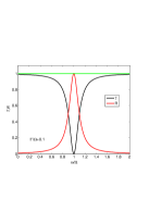
Figure 1: Color online. Transmittance $T=|t|^{2}$ and reflectance $R=|r|^{2}$ as functions of $\omega/\Omega$ for one qubit in a waveguide. The width of resonance is $2\Gamma$.

The expressions (49), (50) coincide with those obtained in Shen05b where one qubit problem has been solved in a configuration space.

From (49) and (50) we see that $t-r=1$. Unlike the general condition (47) it is valid only for one qubit and reflects the continuity of the wavefunction (44) at the point $x=0$.

The probability for the qubit to be excited is given by (43) with $n=1$:

$$\langle 1|\Psi_{Q}\rangle=\lambda R_{11}=\frac{\lambda}{\hbar}\frac{1}{\omega-\Omega+i\Gamma}$$ (51)

V.2 Two qubits in a waveguide

V.2.1 Spectral properties of effective Hamiltonian

Here we consider the first nontrivial example that exhibits superradiant transition: the two noninteracting qubits in a waveguide . The qubits are positioned at the points $x_{1}=-d/2$ and $x_{2}=+d/2$, respectively, with a distance $d$ between them. The Q- subspace is formed by two state vectors $|1\rangle\equiv|e_{1},g_{2},0\rangle$ and $|2\rangle\equiv|g_{1},e_{2},0\rangle$. According to (39) the matrix of effective Hamiltonian is as follows:

$${H_{eff}}=\left({\begin{array}[]{*{20}{c}}{\varepsilon-i\hbar{\Gamma_{1}}}&{-i\hbar\sqrt{{\Gamma_{1}}{\Gamma_{2}}}{e^{ikd}}}\\ {-i\hbar\sqrt{{\Gamma_{1}}{\Gamma_{2}}}{e^{ikd}}}&{-\varepsilon-i\hbar{\Gamma_{2}}}\end{array}}\right)$$ (52)

where $\varepsilon=\frac{\hbar}{2}(\Omega_{1}-\Omega_{2})$, and $\Gamma_{i},(i=1,2)$ are defined in (40).

From the matrix (52) we can find the complex energies of the Q- system from the equation (18), where $\rm E={\rm{}}\hbar\widetilde{\omega}-\frac{\hbar}{2}\left({{\Omega_{1}}+{\Omega_{2}}}\right)$. For two qubit case the equation (18) gives two poles in the complex $\widetilde{\omega}$ plane as the function of physical frequency $\omega$.

$$\tilde{\omega}=\frac{{{\Omega_{1}}+{\Omega_{2}}}}{2}-i\frac{{{\Gamma_{1}}+{\Gamma_{2}}}}{2}\pm$$

$$\sqrt{\frac{1}{4}{{\left({{\Omega_{1}}-{\Omega_{2}}+i[{\Gamma_{2}}-{\Gamma_{1}}]}\right)}^{2}}-{\Gamma_{1}}{\Gamma_{2}}{e^{2ikd}}}$$ (53)

From this expression it follows that the positions of resonances and their widths depend on the frequency $\omega$ of incident photon ($k=\omega/v_{g}$). This is a common feature of non Markovian behavior if the number of qubits is more than one.

For identical noninteracting qubits $\Omega_{1}=\Omega_{2}=\Omega$, $\Gamma_{1}=\Gamma_{2}=\Gamma$ we obtain from (V.2.1)

$$\widetilde{\omega}=\Omega-i\Gamma\pm i\Gamma{e^{ikd}}$$ (54)

In the complex $\widetilde{\omega}$ plane the roots are as follows

$${\mathop{\rm Re}}\widetilde{\omega}\equiv\widetilde{E}=\Omega\mp\Gamma\sin kd$$ (55)

$${\mathop{\rm Im}}\widetilde{\omega}\equiv\widetilde{\Gamma}=-\Gamma\left({1\mp\cos kd}\right)$$ (56)

From (55) and (56) we obtain the relation between the real and imaginary part of the roots

$${\left({\widetilde{E}-\Omega}\right)^{2}}+{\left({\widetilde{\Gamma}+\Gamma}\right)^{2}}={\Gamma^{2}}$$ (57)

It is remarkable that this relation does not depend on the $k$, i. e., on the running frequency $\omega$. In the plane $(\widetilde{\Gamma},\widetilde{E})$ all solutions of eq. (57) lie at the circle centered in the point $-\Gamma,\Omega$ with radius equal to $\Gamma$.

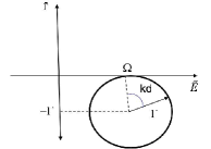
Figure 2: The relation between real and imaginary part of the roots in the complex $\widetilde{\omega}$ plane. For every $kd$ there are two roots which lie on the circle at the opposite points

In the long wavelength limit $(kd<<1)$ we obtain from (54) two poles

$${\widetilde{\omega}_{+}}=\Omega+\Gamma\frac{\omega}{{{{\rm{v}}_{g}}}}d-i2\Gamma$$

$${\widetilde{\omega}_{-}}=\Omega-\Gamma\frac{\omega}{{{{\rm{v}}_{g}}}}$$

We see that in this approximation one of the states absorbs the width of two qubits. With the increase of $\Gamma$ two states repel each other. This is also holds if $kd$ is integer multiple of $\pi$: one state becomes stationary while the width of the other state is $2\Gamma$. However, this case is valid only for particular values of the running frequency $\omega_{n}=\pi nv_{g}/d$, $(n=1,2...)$.

V.2.2 Calculation of microwave transmission

In order to find transmission and reflection factors $t$ and $r$, it is necessary to calculate the matrix $R_{m,n}$, ($m,n=1,2$) which is the inverse of the matrix $(E-H_{eff})_{m,n}$, where the physical energy $E=\hbar\omega-\hbar(\Omega_{1}+\Omega_{2})/2$, and the elements of the matrix $(H_{eff})_{m,n}$ are given in (52). Direct calculations yield for $R_{m,n}$ the following result:

$${R_{m,n}}=\frac{1}{{\hbar{D_{2}}(\omega)}}\left({\begin{array}[]{*{20}{c}}{\omega-{\Omega_{2}}+i{\Gamma_{2}}}&{-i\sqrt{{\Gamma_{1}}{\Gamma_{2}}}{e^{ikd}}}\\ {-i\sqrt{{\Gamma_{1}}{\Gamma_{2}}}{e^{ikd}}}&{\omega-{\Omega_{1}}+i{\Gamma_{1}}}\end{array}}\right)$$ (58)

where

$${D_{2}}(\omega)=\left[{\omega-{\Omega_{2}}+i{\Gamma_{2}}}\right]\left[{\omega-{\Omega_{1}}+i{\Gamma_{1}}}\right]+{\Gamma_{1}}{\Gamma_{2}}{e^{i2kd}}$$ (59)

Finally, according to prescriptions in (45) and (46) we obtain $t$ and $r$ in terms of running frequency $\omega$:

$$t_{2}=\frac{{(\omega-{\Omega_{1}})(\omega-{\Omega_{2}})}}{{\left[{\omega-{\Omega_{2}}+i{\Gamma_{2}}}\right]\left[{\omega-{\Omega_{1}}+i{\Gamma_{1}}}\right]+{\Gamma_{1}}{\Gamma_{2}}{e^{2ikd}}}}$$ (60)

$$r_{2}=-i\frac{{\left\{{{e^{ikd}}{\Gamma_{1}}\left[{\omega-{\Omega_{2}}-i{\Gamma_{2}}}\right]}\right.+\left.{{e^{-ikd}}{\Gamma_{2}}\left[{\omega-{\Omega_{1}}+i{\Gamma_{1}}}\right]}\right\}}}{{\left[{\omega-{\Omega_{2}}+i{\Gamma_{2}}}\right]\left[{\omega-{\Omega_{1}}+i{\Gamma_{1}}}\right]+{\Gamma_{1}}{\Gamma_{2}}{e^{2ikd}}}}$$ (61)

For identical qubits we obtain from (60), (61):

$$t_{2}=\frac{{{{(\omega-\Omega)}^{2}}}}{D_{2}^{id}(\omega)}$$ (62)

$$r_{2}=-i\frac{{2\Gamma[(\omega-\Omega)\cos kd+\Gamma\sin kd]}}{D_{2}^{id}(\omega)}$$ (63)

where

$$D_{2}^{id}(\omega)={{{{(\omega-\Omega+i\Gamma)}^{2}}+{\Gamma^{2}}{e^{2ikd}}}}$$ (64)

As is seen from these expressions the form of the transmission and reflection spectra depend on the inter qubit distance $d$. In the long wavelength limit we obtain from (62) and (63):

$$t_{2}=\frac{{\omega-\Omega}}{{\omega-\Omega+i2\Gamma}}$$ (65)

$$r_{2}=\frac{-i2\Gamma}{{\omega-\Omega+i2\Gamma}}$$ (66)

The expressions (65), (66) are identical to the one qubit case (49), (50) with the only exception. For two identical qubits the resonance width is twice the resonance width for one qubit, which is clear signature of superradiance transition which corresponds to a coherent symmetric superposition $({\Psi_{Q})_{S}}=a\left({\left|1\right\rangle+\left|2\right\rangle}\right)$, whete the quantity $a$ is given in the next subsection.

Below we show several plots of transmission and reflection amplitudes for different values of $k_{0}d$, where $k_{0}=\Omega/v_{g}$. The plots are calculated for two identical qubits from (62) and (63). The points of the full transmission corresponds to zeros of the numerator of the expression (63). Hence, the full transmission is observed at the points where the reflection is exactly equal to zero.

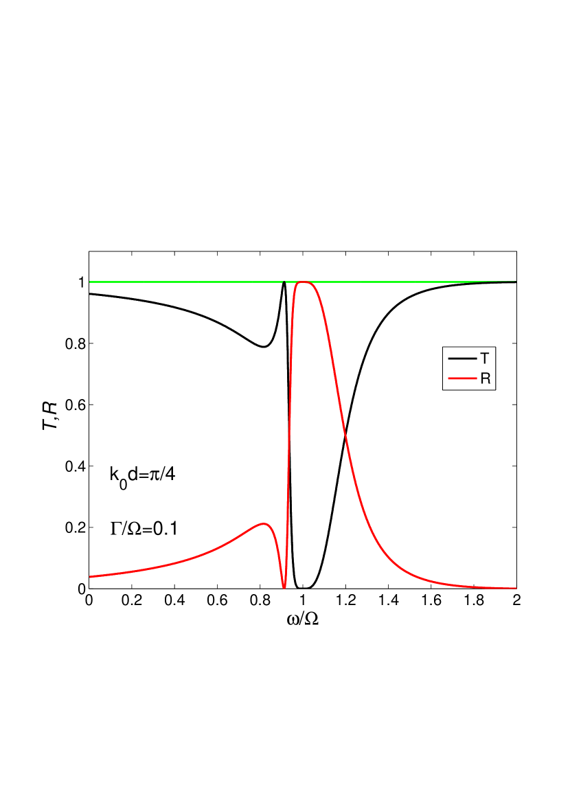
a)

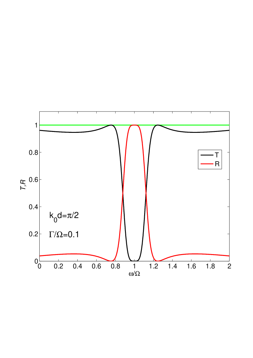
b)

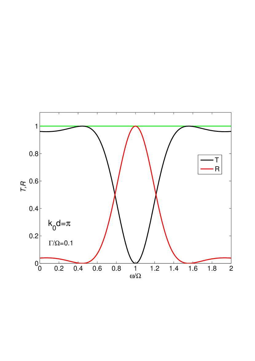
c)

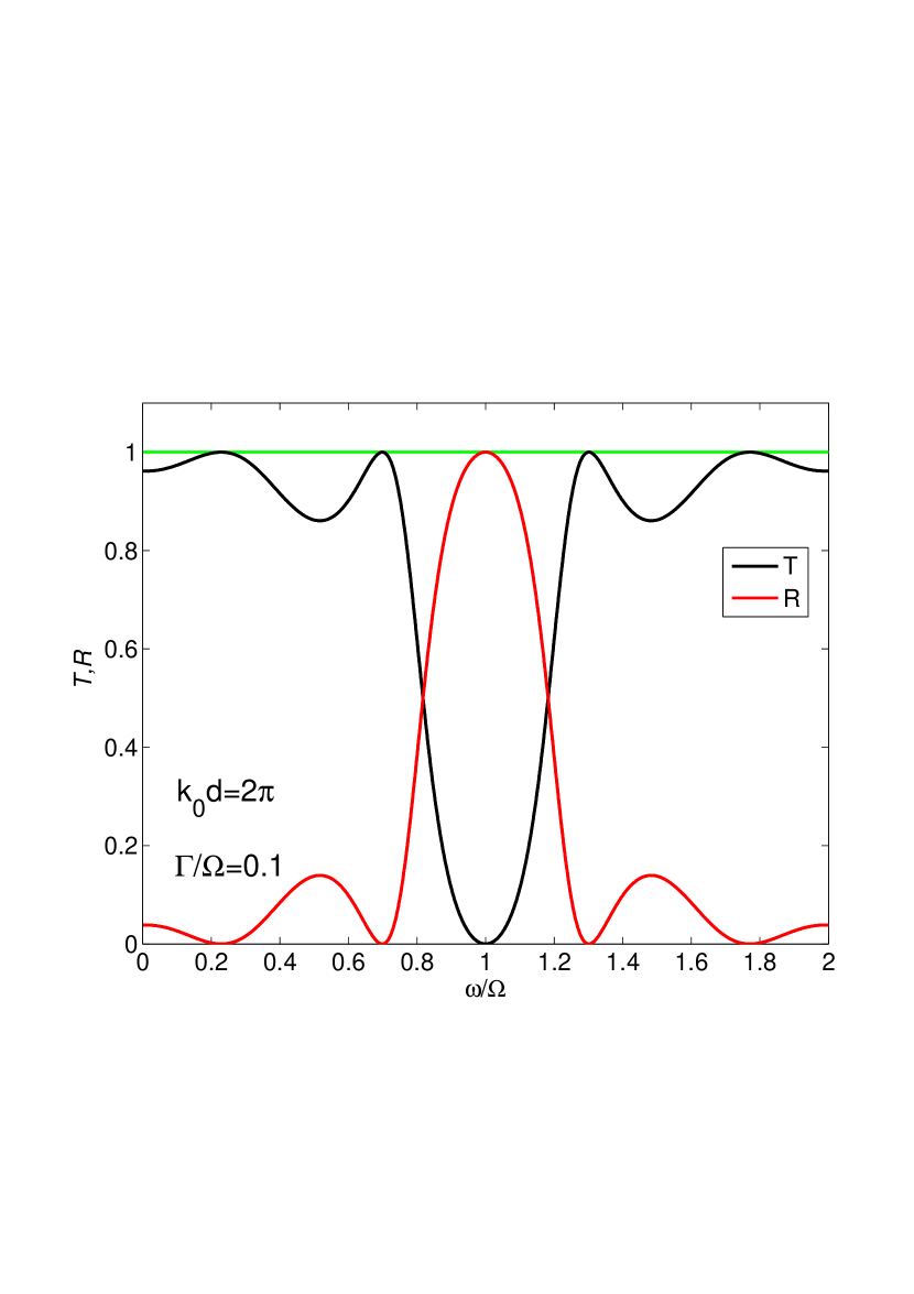
d)

Figure 3: Color online. The dependence of transmission (black) and reflection (red) amplitudes on the frequency of incident photon, $\omega/\Omega$ for different values of $k_{0}d$ for two identical qubits.

V.2.3 Photon mediated entanglement of two qubits

For two qubits the structure of the function $\Psi_{Q}$ (42) within a subspace of qubit states $|1\rangle$ and $|2\rangle$ is a linear superposition of the two two-qubit states $\Psi_{Q}=a\left|1\right\rangle+b\left|2\right\rangle$, where, in general, $a$ and $b$ depend on the physical frequency $\omega$. For two identical qubits we obtain a general expression which describes the frequency dependent entanglement of two two-qubit states:

$$\Psi_{Q}=\frac{\lambda e^{ikd/2}}{D_{2}^{id}(\omega)}\left([(\omega-\Omega+i\Gamma)e^{-ikd}-i\Gamma e^{ikd}]|1\rangle\right.\\ +\left.(\omega-\Omega)|2\rangle\right)$$ (67)

In the long wavelength limit $kd<<1$ the maximally entangled superradiant state which corresponds to a coherent symmetric superposition is formed:

$$({\Psi_{Q})_{S}}=\frac{\lambda}{\omega-\Omega+2i\Gamma}\left({\left|1\right\rangle+\left|2\right\rangle}\right)$$ (68)

The transmission and reflection in this case are given by the expressions (65) and (66). The resonance line of superradiant state is directly given as the line of reflection factor (66).

However, for arbitrary values of $kd$ maximally entangled states are formed only for particular values of the frequency $\omega$. For example, if $kd\equiv\omega d/v_{g}=n\pi$ ($n=1,2,...$) we obtain from (67) the expression

$$\Psi_{Q}=\frac{\lambda i^{n}}{\omega_{n}-\Omega+2i\Gamma}\left[(-1)^{n}|1\rangle+|2\rangle\right]$$ (69)

where $\omega_{n}=n\pi v_{g}/d$.

For on resonant excitation ($\omega=\Omega$) and $k_{0}d\neq n\pi$, where $k_{0}=\Omega/v_{g}$ we get from (67) unentangled state $\Psi_{Q}=i\left(\lambda/{\Gamma}\right)e^{-ik_{0}d/2}|1\rangle$. In this case we observe a full reflection with only the first qubit being excited.

V.2.4 Resonances in two- qubit system

As it follows from the results of subsection III.0.2 the resonances (their energies and widths) in multi-qubit system are given by the roots of equation (18). The widths of these resonances define, in general, the decay rates of the qubit wavefunction $\Psi_{Q}$ (30).

For two qubits these roots, which are labelled below as $\widetilde{\omega}_{1},\widetilde{\omega}_{2}$, are given in (V.2.1). The denominator (59) can then be written as $D_{2}(\omega)=\left[\omega-\widetilde{\omega}_{1}(\omega)\right]$ $\left[\omega-\widetilde{\omega}_{2}(\omega))\right]$. Hence, the resonance frequencies of the incident photon are given by the roots of, in general, nonlinear equations $\omega=\rm{Re}[\widetilde{\omega}_{1}(\omega)]$, $\omega=\rm{Re}[\widetilde{\omega}_{2}(\omega)]$. These equations imply that the resonance energies $\rm{Re}[\widetilde{\omega}_{1}(\omega)]$, $\rm{Re}[\widetilde{\omega}_{2}(\omega)]$ (and their widths $\rm{Im}[\widetilde{\omega}_{1}(\omega)]$, $\rm{Im}[\widetilde{\omega}_{2}(\omega)]$) depend on the frequency of incident photon, which comes in (V.2.1) via the the wave vector $k=\omega/v_{g}$. This is a general feature of non Markovian behavior when the photon mediated interaction between qubits is not instantaneous and the retardation effects have to be included. In our method the retardation effects are automatically included since the quantity $kd$ explicitly enters the expressions for the transmission and reflection factors. Markovian case corresponds to long wavelength limit, $kd<<1$ when the propagation time of photons between the qubits can be neglected and, hence, the qubits interact instantaneously.

It is important that the resonance widths are directly related to the lifetime of qubit superposition state (67) since they define the poles of denominator $D_{2}^{id}(\omega)$ in the low half of the complex energy plane.

Below we discuss the experimental detection of resonance frequencies and their widths. One of the way is to Fourier transform the data collected in photon-photon correlation measurements Zheng13 . However, the experiments of this type demand serious attention to optimizing both the measuring system and experimental conditions. Here we suggest to extract resonance parameters from directly measured transmission data. As an example we consider here two identical qubits.

The resonance structure of transmission (62) and reflection (63) is masked by the frequency dependence of their numerators. This obstacle can be overcome by appropriate processing of the output transmission data. In order the resonance peaks to reveal themselves we propose to divide the transmission (62) by the factor $[(\omega-\Omega)/\Omega]^{2}$. Thus, we analyze the spectral function $S(\omega)$, which contains pure resonance structure:

$$S(\omega)=\frac{\Omega^{2}}{(\omega-\Omega+i\Gamma)^{2}+\Gamma^{2}e^{2i\frac{\omega}{\Omega}k_{0}d}}$$ (70)

The plot of $S(\omega)$ which exhibits two peaks corresponding to solutions of two equations (see (55))

$$\omega=\Omega\pm\Gamma\sin\left(\frac{\omega}{\Omega}k_{0}d\right)$$ (71)

is shown together with transmission at Fig.4 for $k_{0}d=\pi/2,\Gamma/\Omega=0.2$.

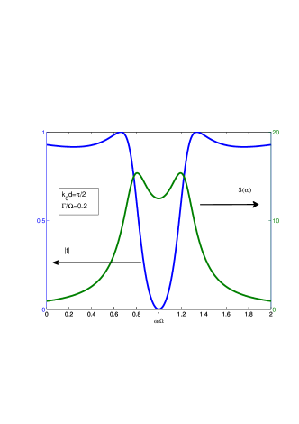
Figure 4: Color online. Frequency dependence of the transmission (left axis, black line) and spectral function (right axis, green line)for two identical qubits. $k_{0}d=\pi/2,\Gamma/\Omega=0.2$.

We notice that the positions of these peaks at the frequency axis do not coincide with the points of the full transmission. The latter points are located exactly where the reflection is zero. This is well illustrated in Fig.5 and Fig.6 where the transmission pattern and corresponding resonance spectrum are shown for $k_{0}d=5.5\pi,\Gamma/\Omega=0.2$.

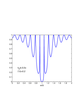
Figure 5: Color online. Transmission pattern for two identical qubits. $k_{0}d=5.5\pi,\Gamma/\Omega=0.2$.

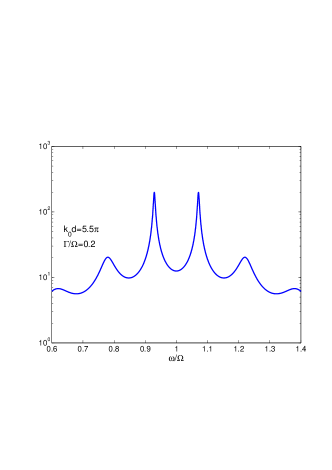
Figure 6: Color online. Frequency dependence of the spectral function for two identical qubits. $k_{0}d=5.5\pi,\Gamma/\Omega=0.2$. The $y$-axis is in log scale

The transmission pattern exhibits $12$ points of the full transmission within the range of the frequency axis while there are only six resonances at the frequencies which are given by the roots of equation (71): $\omega/\Omega=0.805,0.866,0.929,1.070,1,133,1.194$ with the corresponding widths $\widetilde{\Gamma}/\Omega=-0.155,-0.349,-0.013,-0.013,-0.349,-0.155$ Only four resonances which are sufficiently close to real axis are visible in Fig. 6. It is worth noting that there are two resonances with the widths being much smaller the width of individual qubit. Hence, for $k_{0}d=5.5\pi$ these two resonances give the smallest decay rates for two-qubit superposition state (67).

We may conclude that as the distance between qubits, $d$ is increased at fixed $\Gamma$, a number of the roots of (71), which for small $\Gamma$’s lie in the narrow range $\Omega\pm\Gamma$, is also increased, being approximately equal to $k_{0}d/\pi$, while the widths of corresponding peaks are decreased. The latter effect is a direct manifestation of non Markovian behavior.

V.2.5 Photon wave function for two qubits in a waveguide

Photon wave function for two qubits is calculated from (41) with $x_{1}=-d/2,x_{2}=+d/2$ and the matrix $R_{m,n}$ from (58). Outside the qubit array $x>d/2$, $x<-d/2$ the wavefunction is given by (44) with $t$ and $r$ from (60) and (61). Below we write the photon wavefunction for two qubits in the intermediate region $(-d/2<x<+d/2)$:

$${\Psi_{2}}(x)=\frac{{(\omega-{\Omega_{1}})}}{{{D_{2}}(\omega)}}\left({{e^{ikx}}(\omega-{\Omega_{2}}+i{\Gamma_{2}})-i{\Gamma_{2}}{e^{ikd}}{e^{-ikx}}}\right)$$ (72)

It can easily be verified that the wavefunctions (44) and (72) are continuous at the points $x=\pm d/2$. At resonance with the first qubit $(\omega=\Omega_{1})$ photon is reflected from the first qubit and does not penetrate in the inter qubit region $x>-d/2$. However, at resonance with the second qubit $(\omega=\Omega_{2})$ the wave function $\Psi_{2}(x)\neq 0$ at inter qubit region $-d/2<x<d/2$, but $\Psi_{2}(d/2)=0$ as it follows from continuity condition.

From (43) we calculate the probability amplitude for the first or second qubit to be excited.

$$\left\langle{1|{\Psi_{Q}}}\right\rangle=\frac{{{e^{-ikd/2}}}}{{\hbar{D_{2}}(\omega)}}\left[{{\lambda_{1}}\left({\omega-{\Omega_{2}}+i{\Gamma_{2}}}\right)-i{\lambda_{2}}\sqrt{{\Gamma_{1}}{\Gamma_{2}}}{e^{2ikd}}}\right]$$ (73)

$$\left\langle{2|{\Psi_{Q}}}\right\rangle=\frac{{{e^{ikd/2}}}}{{\hbar{D_{2}}(\omega)}}\left[{{\lambda_{2}}\left({\omega-{\Omega_{1}}+i{\Gamma_{1}}}\right)-i{\lambda_{1}}\sqrt{{\Gamma_{1}}{\Gamma_{2}}}}\right]$$ (74)

From the definition of $\Gamma$ (40) we may rewrite (74) as:

$$\left\langle{2|{\Psi_{Q}}}\right\rangle=\frac{{{e^{ikd/2}}}}{{\hbar{D_{2}}(\omega)}}\left[{{\lambda_{2}}\left({\omega-{\Omega_{1}}}\right)}\right]$$

Hence, if the photon is in resonance with the first qubit, the second qubit remains unexcited. If the photon is in resonance with the second qubit, the first qubit is unexcited only if $\Omega_{2}d/v_{g}=\pi$.

V.3 Three qubits in a waveguide

V.3.1 Spectral properties of effective Hamiltonian

Here we consider three noninteracting qubits in a waveguide . The qubits are positioned at the points $x_{1}=-d$, $x_{2}=+d$ and $x_{3}=0$, respectively, with a distance $d$ between adjacent qubits. The Q- subspace is formed by three state vectors $|1\rangle\equiv|e_{1},g_{2},g_{3},0\rangle$, $|2\rangle\equiv|g_{1},e_{2},g_{3},0\rangle$ and $|3\rangle\equiv|g_{1},g_{2},e_{3},0\rangle$. The states $|1\rangle$ and $|2\rangle$ correspond to qubits located at the points $x=\pm d$, respectively. The state $|3\rangle$ is for the qubit placed at the point $x=0$. The $P$-subspace is formed by the vectors $|k\rangle\equiv|g_{1},g_{2},g_{3},k\rangle$. According to (39) the matrix of effective Hamiltonian is as follows:

$${H_{eff}}=\left({\begin{array}[]{*{20}{c}}{{\varepsilon_{1}}-i\hbar{\Gamma_{1}}}&{-i\hbar\sqrt{{\Gamma_{1}}{\Gamma_{2}}}{e^{2ikd}}}&{-i\hbar\sqrt{{\Gamma_{1}}{\Gamma_{3}}}{e^{ikd}}}\\ {-i\hbar\sqrt{{\Gamma_{1}}{\Gamma_{2}}}{e^{2ikd}}}&{{\varepsilon_{2}}-i\hbar{\Gamma_{2}}}&{-i\hbar\sqrt{{\Gamma_{2}}{\Gamma_{3}}}{e^{ikd}}}\\ {-i\hbar\sqrt{{\Gamma_{1}}{\Gamma_{3}}}{e^{ikd}}}&{-i\hbar\sqrt{{\Gamma_{2}}{\Gamma_{3}}}{e^{ikd}}}&{{\varepsilon_{3}}-i\hbar{\Gamma_{3}}}\end{array}}\right)$$ (75)

where $\varepsilon_{i}$ and $\Gamma_{i},(i=1,2,3)$ are defined in (34) and (40), respectively.

The roots of this Hamiltonian in the complex frequency plane are defined by the equation

$$\rm{det}\left(\widetilde{\omega}-\frac{1}{2}\left(\Omega_{1}+\Omega_{2}+\Omega_{3}\right)-H_{eff}/\hbar\right)=0$$

that can be expressed as:

$$\begin{array}[]{l}\left({\tilde{\omega}-{\Omega_{1}}+i{\Gamma_{1}}}\right)\left({\tilde{\omega}-{\Omega_{2}}+i{\Gamma_{2}}}\right)\left({\tilde{\omega}-{\Omega_{3}}+i{\Gamma_{3}}}\right)\\ +\left({\tilde{\omega}-{\Omega_{1}}+i{\Gamma_{1}}}\right){\Gamma_{2}}{\Gamma_{3}}{e^{2ikd}}+\left({\tilde{\omega}-{\Omega_{2}}+i{\Gamma_{2}}}\right){\Gamma_{1}}{\Gamma_{3}}{e^{2ikd}}\\ +\left({\tilde{\omega}-{\Omega_{3}}-i{\Gamma_{3}}}\right){\Gamma_{1}}{\Gamma_{2}}{e^{4ikd}}=0\end{array}$$ (76)

We note that in general the energies and the widths of resonances depend on the physical frequency $\omega$ ($k=\omega/v_{g}$).

For identical qubits ($\Omega_{1}=\Omega_{2}=\Omega_{3}\equiv\Omega$, $\Gamma_{1}=\Gamma_{2}=\Gamma_{3}\equiv\Gamma$) we obtain from (76)

$$\begin{array}[]{l}{\left({\tilde{\omega}-\Omega+i\Gamma}\right)^{3}}+2\left({\tilde{\omega}-\Omega+i\Gamma}\right){\Gamma^{2}}{e^{2ikd}}\\ +\left({\tilde{\omega}-\Omega-i\Gamma}\right){\Gamma^{2}}{e^{4ikd}}=0\end{array}$$ (77)

In the long wavelength limit we find from (77)

$${\left({\tilde{\omega}-\Omega}\right)^{3}}+3i\Gamma{\left({\tilde{\omega}-\Omega}\right)^{2}}=0$$

which gives two resonances with null width and one resonance which absorbs the widths of all three qubits:

$$\widetilde{\omega}_{1,2}=\Omega;\quad\widetilde{\omega}_{3}=\Omega-3i\Gamma$$

We obtain the same result if the running frequency $\omega$ in (77) corresponds to $kd=n\pi,(n=1,2....)$.

The $kd$- dependence of real and imaginary part of three complex roots of equation (77), $\widetilde{\omega}=\rm{Re}\widetilde{\omega}-i\widetilde{\Gamma}$, is shown in Fig.7, where $x=(\rm{Re}\widetilde{\omega}-\Omega)/\Gamma$, $y=(\widetilde{\Gamma}-\Gamma)/\Gamma$. In 3D space ($x,y,z=kd$) three lines of the roots are wound with a variable step onto a cylindrical surface which has two radii, $\Gamma$ and $3\Gamma/2$. So that, in the projection to $x,y$ plane these roots form two circles as shown in Fig.8. Every point on these circles is merged from black and red points of Fig. 7, which belong to the same root.

Figure 7: Color online. The $kd$- dependence of real (a) and imaginary (b) part of three complex roots of equation (77), $\widetilde{\omega}=\rm{Re}\widetilde{\omega}-i\widetilde{\Gamma}$, where $x=(\rm{Re}\widetilde{\omega}-\Omega)/\Gamma$, $y=(\widetilde{\Gamma}-\Gamma)/\Gamma$. The line numbers correspond to real and imaginary parts of three roots of Eq.77.

Figure 8: The projection of the three roots of Eq. 77 to $x,y$ plane, where $x=(\rm{Re}\widetilde{\omega}-\Omega)/\Gamma$, $y=(\widetilde{\Gamma}-\Gamma)/\Gamma$. Every point on this graph are merged from black and red points of Fig. 7, which belong to the same root.

V.3.2 Transmission and reflection spectra for three qubits in a waveguide

Transmission and reflection factors are calculated from (45) and (46), where $m,n=1,2,3$ and $R_{mn}$ is given in Appendix. In the frequency picture with $E=\hbar\omega-\hbar(\Omega_{1}+\Omega_{2}+\Omega_{3})/2$ we obtain for three qubits $t$ and $r$ the following expressions:

$$t_{3}=\frac{{(\omega-{\Omega_{1}})(\omega-{\Omega_{2}})(\omega-{\Omega_{3}})}}{{D_{3}\left(\omega\right)}}$$ (78)

$$r_{3}=-i\frac{{G(\omega)}}{{D_{3}(\omega)}}$$ (79)

where

$$\begin{array}[]{l}D_{3}(\omega)=\left({\omega-{\Omega_{1}}+i{\Gamma_{1}}}\right)\left({\omega-{\Omega_{2}}+i{\Gamma_{2}}}\right)\left({\omega-{\Omega_{3}}+i{\Gamma_{3}}}\right)\\[3.0pt] +\left({\omega-{\Omega_{1}}+i{\Gamma_{1}}}\right){\Gamma_{2}}{\Gamma_{3}}{e^{2ikd}}+\left({\omega-{\Omega_{2}}+i{\Gamma_{2}}}\right){\Gamma_{1}}{\Gamma_{3}}{e^{2ikd}}\\[3.0pt] +\left({\omega-{\Omega_{3}}-i{\Gamma_{3}}}\right){\Gamma_{1}}{\Gamma_{2}}{e^{4ikd}}\end{array}$$ (80)

$$\begin{array}[]{l}G(\omega)={\Gamma_{1}}(\omega-{\Omega_{2}}+i{\Gamma_{2}})(\omega-{\Omega_{3}}+i{\Gamma_{3}}){e^{-2ikd}}\\[3.0pt] +{\Gamma_{2}}(\omega-{\Omega_{1}}+i{\Gamma_{1}})(\omega-{\Omega_{3}}+i{\Gamma_{3}}){e^{2ikd}}\\[3.0pt] +{\Gamma_{3}}(\omega-{\Omega_{1}})(\omega-{\Omega_{2}})+i{\Gamma_{2}}{\Gamma_{3}}(\omega-{\Omega_{1}})\\[3.0pt] +i{\Gamma_{1}}{\Gamma_{3}}(\omega-{\Omega_{2}})-2i{\Gamma_{1}}{\Gamma_{3}}(\omega-{\Omega_{2}}+i{\Gamma_{2}})\\[3.0pt] -2i{\Gamma_{1}}{\Gamma_{2}}(\omega-{\Omega_{3}}){e^{2ikd}}-2i{\Gamma_{3}}{\Gamma_{2}}(\omega-{\Omega_{1}}){e^{2ikd}}\end{array}$$ (81)

For identical qubits we obtain

$$t_{3}=\frac{{{{(\omega-\Omega)}^{3}}}}{{{D_{3}^{id}}\left(\omega\right)}}$$ (82)

$$r_{3}=-i\frac{{{G_{id}}(\omega)}}{{{D_{3}^{id}}(\omega)}}$$ (83)

where $D_{3}^{id}(\omega)$ is calculated in the section 2 of Appendix.

$$\begin{array}[]{l}D_{3}^{id}(\omega)={\left({\omega-\Omega+i\Gamma}\right)^{3}}+2\left({\omega-\Omega+i\Gamma}\right){\Gamma^{2}}{e^{2ikd}}\\[3.0pt] +\left({\omega-\Omega-i\Gamma}\right){\Gamma^{2}}{e^{4ikd}}\end{array}$$ (84)

$$\begin{array}[]{l}G_{id}(\omega)=2\Gamma[(\omega-\Omega)^{2}-\Gamma^{2}]\cos 2kd+\Gamma{(\omega-\Omega)^{2}}+2{\Gamma^{3}}\\[3.0pt] +4{\Gamma^{2}}(\omega-\Omega)\sin 2kd\end{array}$$ (85)

In the long wavelength limit $(kd<<1)$ we obtain from (82) and (83)

$$t_{3}=\frac{{\omega-\Omega}}{{\omega-\Omega+3i\Gamma}}$$ (86)

$$r_{3}=-\frac{{3i\Gamma}}{{\omega-\Omega+3i\Gamma}}$$ (87)

We note that the expressions (86), (87) are valid for a broad range of frequencies satisfying the condition $kd<<1$. However, as $k=\omega/v_{g}$ these expressions are also valid for $kd=n\pi,n=1,2,..$ but only at the fixed frequencies $\omega_{n}=n\pi v_{g}/d$.

As in the two qubits case (65), (66) the expressions (86), (87) are similar to the ones for one qubit (49), (50) but with the width that is three times greater.

Below we show several plots of transmission and reflection amplitudes for different values of $k_{0}d$, where $k_{0}=\Omega/v_{g}$. The plots are calculated for three identical qubits from (82) and (83).

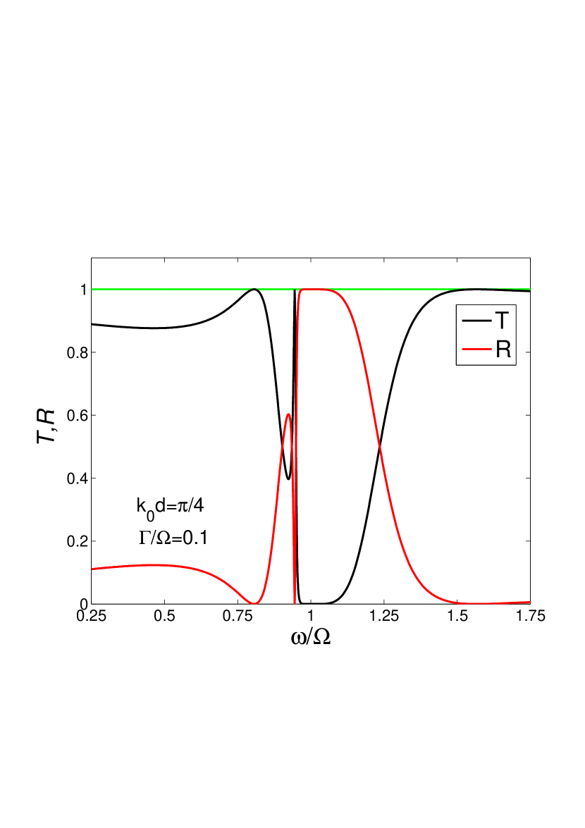
a)

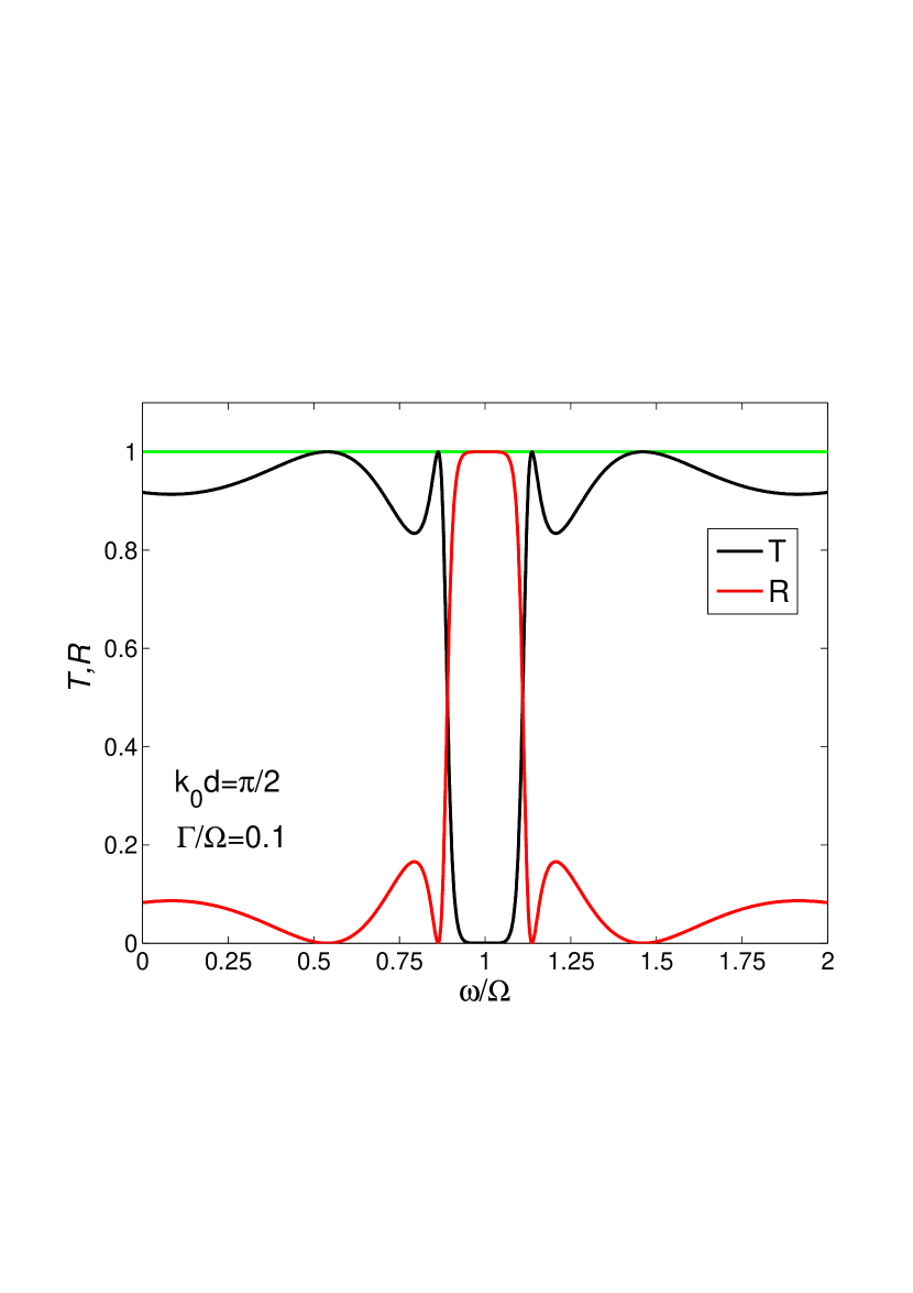
b)

c)

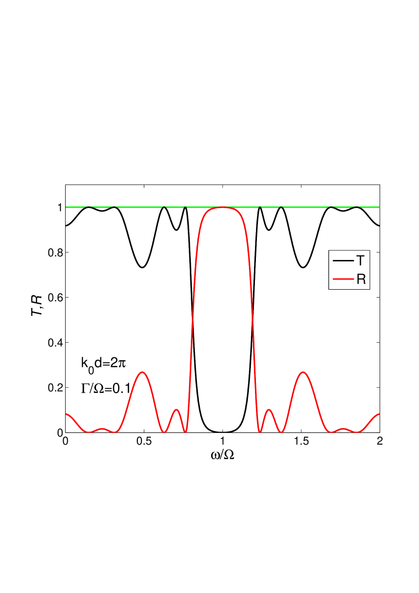
d)

Figure 9: Color online. The dependence of transmission (black) and reflection (red) amplitudes on the frequency of incident photon, $\omega/\Omega$ for different values of $k_{0}d$ for three identical qubits.

V.3.3 Photon mediated entanglement for three qubits

Analogous to two qubit case the function of the qubit system $\Psi_{Q}$ (20) can be written as a linear superposition of the three two-qubit states $\Psi_{Q}=a\left|1\right\rangle+b\left|2\right\rangle+c\left|3\right\rangle$, where, in general, $a$, $b$, and $c$ depend on the physical frequency $\omega$. For three identical qubits we obtain a general expression which describes the frequency dependent entanglement of three three-qubit states:

$$\Psi_{Q}=\frac{\lambda}{D_{3}^{id}(\omega)}\left([(\omega-\Omega+i\Gamma)^{2}e^{-ikd}+\Gamma^{2}e^{ikd}\right.\\ -i\Gamma(\omega-\Omega+i\Gamma)e^{ikd}-i\Gamma(\omega-\Omega-i\Gamma)e^{3ikd}]|1\rangle\\ \left.(\omega-\Omega)^{2}e^{ikd}|2\rangle+(\omega-\Omega)[\omega-\Omega+i\Gamma(1-e^{2ikd})]|3\rangle\right)$$ (88)

In the long wavelength limit $kd<<1$ the maximally entangled superradiant state which corresponds to a coherent symmetric superposition of three three-qubit states is formed:

$$({\Psi_{Q})_{S}}=\frac{\lambda}{\omega-\Omega+3i\Gamma}\left({\left|1\right\rangle+\left|2\right\rangle}+|3\rangle\right)$$ (89)

The transmission and reflection in this case are given by the expressions (86) and (87). The resonance line of superradiant state is directly given as the line of reflection factor (87).

For arbitrary values of $kd$ maximally entangled states are formed only for fixed values of the frequency $\omega$. For example, if $kd\equiv\omega d/v_{g}=n\pi$ ($n=1,2,...$) we obtain from (88) the expression

$$\Psi_{Q}=\frac{\lambda}{\omega_{n}-\Omega+3i\Gamma}\left[(-1)^{n}(|1\rangle+|2\rangle)+|3\rangle\right]$$ (90)

where $\omega_{n}=n\pi v_{g}/d$.

For on resonant excitation ($\omega=\Omega$) and $k_{0}d\neq n\pi$, where $k_{0}=\Omega/v_{g}$ we get from (88) unentangled state $\Psi_{Q}=i\left(\lambda/\Gamma\right)e^{ik_{0}d}|1\rangle$. In this case we observe a full reflection with only the first qubit being excited.

V.3.4 Resonances in three- qubit system

As in the two qubit case, the resonance frequencies in (78) and (79) are given by three equations $\omega=\rm{Re}[\widetilde{\omega}_{1}(\omega)]$, $\omega=\rm{Re}[\widetilde{\omega}_{2}(\omega)]$,$\omega=\rm{Re}[\widetilde{\omega}_{3}(\omega)]$, where $\widetilde{\omega}_{1},\widetilde{\omega}_{2}$ and $\widetilde{\omega}_{3}$ are the roots of equation (76).

The denominator (80) can then be written as $D_{3}(\omega)=\left[\omega-\widetilde{\omega}_{1}(\omega)\right]$ $\left[\omega-\widetilde{\omega}_{2}(\omega))\right]$ $\left[\omega-\widetilde{\omega}_{3}(\omega))\right]$. Hence, the resonance frequencies of the incident photon are given by the roots of, in general, nonlinear equations $\omega=\rm{Re}[\widetilde{\omega}_{1}(\omega)]$, $\omega=\rm{Re}[\widetilde{\omega}_{2}(\omega)]$, $\omega=\rm{Re}[\widetilde{\omega}_{3}(\omega)]$.

Below we consider three identical qubits. Similar to the case of two qubits we define a spectral function by dividing the transmission (82) by the factor $[(\omega-\Omega)/\Omega]^{3}$:

$$S(\omega)=\frac{\Omega^{3}}{D_{3}^{id}(\omega)}$$ (91)

where $D_{3}^{id}(\omega)$ is given in (84).

Below we show the plots of transmission and spectral function $S(\omega)$ which exhibits peaks corresponding to the roots of the equations $\omega=\rm{Re}[\widetilde{\omega}_{i}(\omega)](i=1,2,3)$, where $\widetilde{\omega}_{1},\widetilde{\omega}_{2}$ and $\widetilde{\omega}_{3}$ are the roots of the equation (77). The resonance spectrum for $k_{0}d=\pi/2,\Gamma/\Omega=0.2$ is shown at Fig.10. For this case there are three resonances at the frequencies $\omega/\Omega=0.8,1.0,1.2$ with corresponding half widths $\widetilde{\Gamma}/\Omega=-0.046,-0.40,-0.046$. However, only two resonances which are closest to the frequency axis (with the width $2\widetilde{\Gamma}/\Omega=0.08$), are visible in Fig.10.

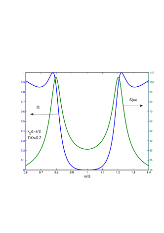
Figure 10: Color online. Frequency dependence of the transmission (left axis, blue line) and spectral function (right axis, green line)for three identical qubits. $k_{0}d=\pi/2,\Gamma/\Omega=0.2$.

With the increase of the inter qubit distance $d$, the number of resonances are also increased, being in the vicinity of $\Omega$ for small $\Gamma$’s. The corresponding transmission pattern and the resonance spectrum are shown in Fiq.11 and Fig.12 for $k_{0}d=5.5\pi,\Gamma/\Omega=0.2$.

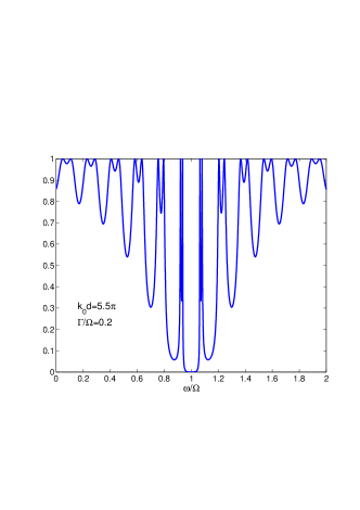
Figure 11: Color online. Transmission pattern for three identical qubits. $k_{0}d=5.5\pi,\Gamma/\Omega=0.2$.

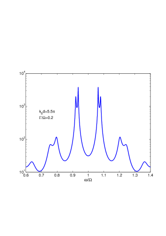
Figure 12: Color online. Frequency dependence of the spectral function for three identical qubits. $k_{0}d=5.5\pi,\Gamma/\Omega=0.2$. The y-axis is in log scale.

In this case in the range $\omega/\Omega=0.6\div 1.4$ there are $13$ resonance frequencies, ten of which are seen in Fig.12. The two highest peaks have the half width $\widetilde{\Gamma}/\Omega=3.5\times 10^{-3}$ and $\widetilde{\Gamma}/\Omega=1.63\times 10^{-2}$, respectively. We note that the widths of some resonances, which define the decay rates of the superposition state (88), are much smaller than the width of individual qubit.

We note that, the points of the full transition which correspond to the zeros of the reflection, do not coincide with the frequencies of the resonances. While for some frequencies the corresponding values can be close to each other, in general, many reflection zeros are out of the range of resonance frequencies.

V.3.5 Photon wave function for three identical qubits in a waveguide

Photon wave function for three identical qubits is calculated from (41) with the matrix $R_{mn}$ defined in (112).

$$\begin{array}[]{l}{\Psi_{3}}(x)={e^{ikx}}-i\hbar\Gamma{e^{ik\left|{x-d}\right|}}\left[{{e^{ikd}}{R_{11}}+{e^{-ikd}}{R_{12}}+{R_{13}}}\right]\\[3.0pt] -i\hbar\Gamma{e^{ik\left|{x+d}\right|}}\left[{{e^{ikd}}{R_{12}}+{e^{-ikd}}{R_{11}}+{R_{13}}}\right]\\[3.0pt] -i\hbar\Gamma{e^{ik\left|x\right|}}\left[{{e^{ikd}}{R_{13}}+{e^{-ikd}}{R_{13}}+{R_{33}}}\right]\end{array}$$ (92)

Outside the qubit array $x<-d$ and $x>d$ the wavefunction (92) is similar to (44), where the transmission $t$ and reflection $r$ are given in (82) and (83). Inside the array we obtain

$${\Psi_{3}}(x)=\frac{{{{(\omega-\Omega)}^{2}}}}{{D_{3}^{id}(\omega)}}\left[{{e^{ikx}}(\omega-\Omega+i\Gamma)-i\Gamma{e^{-ikx}}{e^{2ikd}}}\right]$$ (93)

for $0<x<d$, and

$$\begin{array}[]{l}{\Psi_{3}}(x)=\frac{{(\omega-\Omega)}}{{D_{3}^{id}(\omega)}}\left[{{e^{ikx}}{{(\omega-\Omega+i\Gamma)}^{2}}+{\Gamma^{2}}{e^{2ikd}}}\right.\\[5.0pt] \left.{-i\Gamma{e^{-ikx}}\left[{(\omega-\Omega+i\Gamma)+(\omega-\Omega-i\Gamma){e^{2ikd}}}\right]}\right]\end{array}$$ (94)

for $-d<x<0$.

Similar to the two qubit case, here at the exact resonance ($\omega=\Omega$) the photon wavefunction does not penetrate in the inter qubit region.

In the conclusion to this section we write the probability for the particular qubit in the array to be in excited state. From (43) we obtain:

$$\begin{array}[]{l}\left\langle{1|\Psi_{Q}}\right\rangle=\frac{\lambda}{{\hbar D_{3}^{id}(\omega)}}\left[{{{\left({\omega-\Omega+i\Gamma}\right)}^{2}}{e^{-ikd}}}\right.\\[5.0pt] \quad\quad-i\Gamma\left({\omega-\Omega-i\Gamma}\right){e^{3ikd}}\left.{-i\Gamma\left({\omega-\Omega+2i\Gamma}\right){e^{ikd}}}\right]\end{array}$$ (95)

$$\left\langle{2|\Psi_{Q}}\right\rangle=\frac{\lambda}{\hbar}\frac{{{{\left({\omega-\Omega}\right)}^{2}}}}{{D_{3}^{id}(\omega)}}{e^{ikd}}$$ (96)

$$\left\langle{3|\Psi_{Q}}\right\rangle=\frac{\lambda}{\hbar}\frac{{(\omega-\Omega)}}{{D_{3}^{id}(\omega)}}\left[{\omega-\Omega+i\Gamma\left({1-{e^{2ikd}}}\right)}\right]$$ (97)

We see that at resonance the first qubit only is excited. This is consistent with the above conclusion that at resonance photon does not penetrate beyond the first qubit.

All qubit arrays considered above have a general property: if the photon frequency is equal to the resonance frequency of any qubit in the chain, the transmission signal is absent. We attributed this property to the destructive interference between the input wave and the wave which resulted from the virtual transitions between the qubits and the photon field in the resonator. However, it is not clear to what extent this property can be attributed to uniform distribution of the qubit in the chain with the equal distance between adjacent qubits. The simplest system where we can check this property is the three qubit chain. We made the calculation of the transmission for three different qubits which are positioned at the points $x_{1}=-d_{1}$, $x_{2}=+d_{2}$ and $x_{3}=0$, respectively, with unequal distance between adjacent qubits. It turned out that in this case the transmission is similar to (78) with the just the same numerator, but different denominator, which is given in the Appendix. Hence, we may assume that for nonuniform qubit array the transmission is also zero if the input photon is at resonance with any qubit in the chain.

V.3.6 The manipulation of the photon transmission in three qubit chain

Most of artificial atoms, which are used as qubits, can be addressed individually, so that every qubit frequency, $\Omega_{i}$, in the chain can be tuned from external source. Here we show how this property can be used to manipulate the photon transmission through a waveguide. As an example we consider three non-identical qubits, which are positioned at the points $x_{1}=-d$, $x_{2}=+d$ and $x_{3}=0$, respectively, with a distance $d$ between adjacent qubits. The frequencies $\Omega_{1}$ and $\Omega_{2}$ correspond to qubits at the points $x_{1},x_{2}$, respectively, while $\Omega_{3}$ corresponds to central qubit at the point $x_{3}$. In general, if all three frequencies are different we obtain for long wavelength ($kd<<1$) transmission the plot shown in Fig.13, where for comparison the transmission for identical qubits are also shown. The qubit frequencies are directly given by zeros of the transmission, while two narrow nearby peaks, which lie between qubit frequencies correspond to the full transmission.

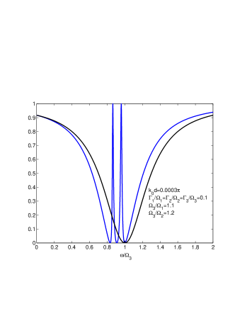
Figure 13: Color online. Transmission for three non-identical qubits (blue line). For comparison the transmission for identical qubits is also shown (black line)

Suppose now that the frequencies of the left and right qubit are equal ($\Omega_{1}=\Omega_{2}\equiv\Omega$) and we manipulate the frequency of the central qubit, $\Omega_{3}$. Then we obtain the picture like the one shown in Fig.14. By changing the qubit frequency $\Omega_{3}$ we may move the frequency of the transmission resonance between $\Omega$ and $\Omega_{3}$ and manipulate its width. When $\Omega_{3}$ becomes equal to $\Omega$ the transmission signal disappear.

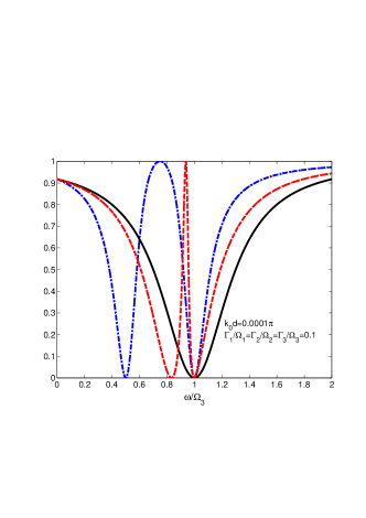
Figure 14: Color online. Transmission for three qubits, two of which are identical. Dashed (red) line: $\Omega_{3}/\Omega_{1}=\Omega_{3}/\Omega_{2}=1.2$. Dash-dotted (blue) line: $\Omega_{3}/\Omega_{1}=\Omega_{3}/\Omega_{2}=2$. For comparison the transmission for identical qubits is also shown by solid (black) line.

V.4 $N$ qubits in a waveguide

In principle the transmission and reflection for any number of qubits can be found from general expressions (45) and (46). For a chain of $N$ identical homogeneously distributed two level atoms the analytical expression for the 1D transmission was found in Tsoi08 . While in general case it is not easy to find analytical solutions for $N$ qubits, nevertheless, from previous calculations of the transmission for one, (49), two, (60), and three (78) qubits, we may guess the general structure of the transmission for $N$ qubits in a waveguide:

$${t_{N}}=\frac{{\prod\limits_{n=1}^{N}{(\omega-{\Omega_{n}})}}}{{{D_{N}}(\omega)}}$$ (98)

where

$${D_{N}}(\omega)=\det\left({\omega-\frac{1}{2}\sum\limits_{i=1}^{N}{{\Omega_{i}}}-{H_{eff}}/\hbar}\right)$$ (99)

As for the spectral properties of the effective Hamiltonian, we can assert that the secular equation $\rm{det}$$(E-H_{eff})$ has $N$ poles in the low half plain of the complex energy. For identical qubits in the long wavelength limit there are $N-1$ stable states with $\widetilde{\omega}=\Omega$ and one resonance $\widetilde{\omega}=\Omega-iN\Gamma$ which absorbs all the widths of individual qubits:

$$t_{N}=\frac{{\omega-\Omega}}{{\omega-\Omega+iN\Gamma}}$$ (100)

$$r_{N}=-\frac{{iN\Gamma}}{{\omega-\Omega+iN\Gamma}}$$ (101)

VI conclusion

In this paper we develop a new technique for the investigation of the photon transport through multiple qubit array in a 1D waveguide. The technique is based on the projection operators formalism and non Hermitian approach, which is known to be a successful tool in some fields of nuclear physics and condensed matter. We considered in detail the one photon transport for two and three qubits in a waveguide, and made some conclusions for $N$ qubit case. We showed that the interaction of qubits with a photon field results in the frequency dependent superposition of the qubit states. We investigated in detail the resonance spectra for two and three qubits and showed that in non Markovian case ($kd>>1$) the resonance widths, which define the decay rates of the superposition state, can be much smaller than the decay width of individual qubit.

We also showed that in the long wavelength limit for uniformly distributed array of identical qubits a coherent superradiance state is formed with the width being equal to the sum of the widths of spontaneous transitions of N individual qubits. Within the framework of our method it is not difficult to account for the decay of the qubit states to the modes other than the waveguide continuum. It can be done by simply adding an imaginary term in the qubit energy level, $\Omega_{n}\rightarrow\Omega_{n}-i\Gamma_{n}^{\prime}$.

The approach developed in the paper can be easily generalized to include the exchange interaction $H_{J}$ between nearest neighbor qubits:

$${H_{J}}=\hbar\sum\limits_{i=1}^{N}{{J_{i}}\left({\sigma_{+}^{i}\sigma_{-}^{i+1}+\sigma_{+}^{i+1}\sigma_{-}^{i}}\right)}$$ (102)

For this case it is necessary to change only the matrix of effective Hamiltonian (39):

$$\left\langle{m}\right|{H_{eff}}\left|{n}\right\rangle=\varepsilon_{m}\delta_{m,n}+\hbar J_{n-1}\delta_{m,n-1}+\hbar J_{n}\delta_{m,n+1}\\ -i\hbar(\Gamma_{m}\Gamma_{n})^{1/2}e^{ik|d_{mn}|}$$ (103)

The results obtained in the paper are of general nature and can be applied to any type of qubits. The specific properties of the qubit are encoded in only two parameters: the qubit energy $\Omega$ and the rate of spontaneous emissin $\Gamma$. For example, for a superconducting flux qubit $\,\Omega=\sqrt{\varepsilon^{2}+\Delta^{2}}$ where $\varepsilon$ is an external parameter which by virtue of external magnetic flux, $\Phi_{X}$ controls the gap between ground and excited states Wal00 , and the quantity $\Delta$ is the qubit’s gap at the degeneracy point ($\varepsilon=0$). The rate of spontaneous emission $\Gamma=g\Delta/\Omega$ Om10 , where $g$ is the qubit- waveguide coupling.

*

Appendix A

A.1 The calculation of integral $J(x_{m},x_{n})$(37)

In (37) the energies $E_{q}$ and $E_{k}$ are the energies of incident photon $|q\rangle$ ($|k\rangle$) plus the energy of $N$ qubits in the ground state. Hence, $E_{q}-E_{k}=\hbar(\omega_{q}-\omega_{k})$. For (37) we, therefore, have

$$J(x_{m},x_{n})=\frac{1}{\hbar}\int\limits_{-\infty}^{+\infty}{dk\frac{{{e^{ikd_{mn}}}}}{{{\omega_{q}}-{\omega_{k}}+i\varepsilon}}}$$ (104)

The main contribution to this integral comes from the region ${\omega_{k}}\approx{\omega_{q}}$. Since $\omega_{k}$ is the even function of $k$, the poles of the integrand (104) in the $k$ plane are located near the points $k\approx\pm q$. For an arbitrary frequency $\omega_{q}$ that is away from the cutoff of the dispersion, with the corresponding wave vector $\pm q$ , we approximate $\omega_{k}$ around $+q$ and $-q$ as

$${\omega_{k}}\approx{\omega_{q}}+(k-q){\left.{\frac{{d{\omega_{k}}}}{{dk}}}\right|_{k=+q}}={\omega_{q}}+(k-q){{\mathop{\rm v}\nolimits}_{g}}$$ (105)

$${\omega_{k}}\approx{\omega_{q}}+(k+q){\left.{\frac{{d{\omega_{k}}}}{{dk}}}\right|_{k=-q}}={\omega_{q}}-(k+q){{\mathop{\rm v}\nolimits}_{g}}$$ (106)

Near the poles the denominator in (104) takes the form:

$$-{{\mathop{\rm v}\nolimits}_{g}}(k-q)+i\varepsilon$$ (107)

$${{\mathop{\rm v}\nolimits}_{g}}(k+q)+i\varepsilon$$ (108)

Therefore, one pole is located in the upper half of the $k$ plane, $k=q+i\varepsilon$, the other pole is located in the lower half of the $k$ plane, $k=-q-i\varepsilon$. For positive $d_{mn}$, when calculating the integral (104) we must close the path in the upper plane. For negative $d_{mn}$ the path should be closed in lower plane. Thus, we obtain:

$$J(x_{m},x_{n})=-\frac{{2\pi i}}{\hbar v_{g}}{e^{ik\left|d_{mn}\right|}}$$ (109)

A.2 Calculation of the $R$ matrix for three qubits in a waveguide

The matrix $R_{m,n}$, ($m,n=1,2,3$) is calculated as the inverse of the matrix $(E-H_{eff})_{m,n}$, the elements of which can be found from (75). The matrix $R_{m,n}$ is symmetric so that $R_{12}=R_{21},R_{13}=R_{31},R_{23}=R_{32}$. Direct calculations yield for $R_{m,n}$ the following result:

$$\begin{array}[]{l}{D_{3}}(E){R_{11}}=\left({E-{\varepsilon_{2}}+i\hbar{\Gamma_{2}}}\right)\left({E-{\varepsilon_{3}}+i\hbar{\Gamma_{3}}}\right)\\ +{\hbar^{2}}{\Gamma_{2}}{\Gamma_{3}}{e^{2ikd}}\\ {D_{3}}(E){R_{22}}=\left({E-{\varepsilon_{1}}+i\hbar{\Gamma_{2}}}\right)\left({E-{\varepsilon_{3}}+i\hbar{\Gamma_{3}}}\right)\\ +{\hbar^{2}}{\Gamma_{1}}{\Gamma_{3}}{e^{2ikd}}\\ {D_{3}}(E){R_{33}}=\left({E-{\varepsilon_{2}}+i\hbar{\Gamma_{2}}}\right)\left({E-{\varepsilon_{1}}+i\hbar{\Gamma_{3}}}\right)\\ +{\hbar^{2}}{\Gamma_{1}}{\Gamma_{2}}{e^{4ikd}}\\ {D_{3}}(E){R_{12}}=-\left({E-{\varepsilon_{3}}+i\hbar{\Gamma_{3}}}\right)i\hbar\sqrt{{\Gamma_{1}}{\Gamma_{2}}}{e^{2ikd}}\\ {-{\hbar^{2}}\sqrt{{\Gamma_{1}}{\Gamma_{2}}}{\Gamma_{3}}{e^{2ikd}}}\\ {D_{3}}(E){R_{13}}=-\left({E-{\varepsilon_{2}}+i\hbar{\Gamma_{2}}}\right)i\hbar\sqrt{{\Gamma_{1}}{\Gamma_{3}}}{e^{ikd}}\\ -{\hbar^{2}}\sqrt{{\Gamma_{1}}{\Gamma_{3}}}{\Gamma_{2}}{e^{3ikd}}\\ {D_{3}}(E){R_{23}}=-\left({E-{\varepsilon_{1}}+i\hbar{\Gamma_{1}}}\right)i\hbar\sqrt{{\Gamma_{2}}{\Gamma_{3}}}{e^{ikd}}\\ -{\hbar^{2}}\sqrt{{\Gamma_{2}}{\Gamma_{3}}}{\Gamma_{1}}{e^{3ikd}}\end{array}$$ (110)

where $D_{3}(E)=\rm{det}\left(\emph{E}-\emph{H}_{eff}\right)_{mn}$:

$$\begin{array}[]{l}{D_{3}}(E)=\left({E-{\varepsilon_{1}}+i\hbar{\Gamma_{1}}}\right)\left({E-{\varepsilon_{2}}+i\hbar{\Gamma_{2}}}\right)\left({E-{\varepsilon_{3}}+i\hbar{\Gamma_{3}}}\right)\\[3.0pt] +\left({E-{\varepsilon_{1}}+i\hbar{\Gamma_{1}}}\right){\hbar^{2}}{\Gamma_{2}}{\Gamma_{3}}{e^{2ikd}}+\\[3.0pt] \left({E-{\varepsilon_{2}}+i\hbar{\Gamma_{2}}}\right){\hbar^{2}}{\Gamma_{1}}{\Gamma_{3}}{e^{2ikd}}+\left({E-{\varepsilon_{3}}-i\hbar{\Gamma_{3}}}\right){\hbar^{2}}{\Gamma_{1}}{\Gamma_{2}}{e^{4ikd}}\end{array}$$ (111)

and the quantities $\varepsilon_{i}(i=1,2,3)$ are defined in (34).

At the end of this subsection we write down from (110) the matrix $R_{m,n}$ for three identical qubits.

$$\begin{array}[]{l}\hbar D_{3}^{id}(\omega){R_{11}}={\left({\omega-\Omega+i\Gamma}\right)^{2}}+{\Gamma^{2}}{e^{2ikd}}\\ \hbar D_{3}^{id}(\omega){R_{33}}={\left({\omega-\Omega+i\Gamma}\right)^{2}}+{\Gamma^{2}}{e^{4ikd}}\\ \hbar D_{3}^{id}(\omega){R_{12}}=-i\Gamma\left({\omega-\Omega}\right){e^{2ikd}}\\ \hbar D_{3}^{id}(\omega){R_{13}}=-i\Gamma\left({\omega-\Omega+i\Gamma}\right){e^{ikd}}-{\Gamma^{2}}{e^{3ikd}}\\ R_{22}=R_{11},R_{23}=R_{13}=R_{31}=R_{32},R_{21}=R_{12}\end{array}$$ (112)

where

$$\begin{array}[]{l}D_{3}^{id}(\omega)={\left({\omega-\Omega+i\Gamma}\right)^{3}}+2{\Gamma^{2}}\left({\omega-\Omega+i\Gamma}\right){e^{2ikd}}\\[3.0pt] +{\Gamma^{2}}\left({\omega-\Omega-i\Gamma}\right){e^{4ikd}}\end{array}$$ (113)

A.3 The transmission for three qubit chain with unequal distance between each other

Here we consider three different qubits which are positioned at the points $x_{1}=-d_{1}$, $x_{2}=+d_{2}$ and $x_{3}=0$, respectively, with $d_{1}\neq d_{2}$. The calculations yields the result:

$$t_{3}=\frac{{(\omega-{\Omega_{1}})(\omega-{\Omega_{2}})(\omega-{\Omega_{3}})}}{{F\left(\omega\right)}}$$ (114)

where

$$\begin{array}[]{l}F(\omega)={U_{1}}{U_{2}}{U_{3}}+i{\Gamma_{1}}{\Gamma_{2}}{\Gamma_{3}}\left({{e^{2ik{d_{1}}}}+{e^{2ik{d_{2}}}}-{e^{2ik({d_{1}}+{d_{2}})}}-1}\right)\\[3.0pt] +{U_{3}}{\Gamma_{1}}{\Gamma_{2}}\left({{e^{2ik{d_{1}}+2ik{d_{2}}}}-1}\right)+{U_{1}}{\Gamma_{2}}{\Gamma_{3}}\left({{e^{2ik{d_{2}}}}-1}\right)\\[3.0pt] +{U_{2}}{\Gamma_{1}}{\Gamma_{3}}\left({{e^{2ik{d_{1}}}}-1}\right)+i{U_{1}}{U_{2}}{\Gamma_{3}}+i{U_{1}}{U_{3}}{\Gamma_{2}}+i{U_{2}}{U_{3}}\Gamma\end{array}$$ (115)

$$U_{1}=\omega-\Omega_{1};\,U_{2}=\omega-\Omega_{2};\,U_{3}=\omega-\Omega_{3}$$

The equation (114) is similar to (78) with the same numerator but different denominator.

References

- (1) I. Buluta, S. Ashhab, F. Nori, Natural and artificial atoms for quantum computation. Rep. Progr. Phys. 74, 104401 (2011).
- (2) J.Q. You, F. Nori, Atomic physics and quantum optics using superconducting circuits. Nature 474, 589 (2011).
- (3) I. Buluta, F. Nori, Quantum Simulators. Science 326, 108 (2009).
- (4) Yao-Lung L. Fang and H. U. Beranger, Wavegude QED: Power spectra and correlations of two photons scattered off multiple distant qubits and a mirror. Phys. Rev. A91, 053845 (2015).
- (5) A. Blais, R-S. Huang, A. Wallraff, S. M. Girvin and R. J. Schoelkopf, Cavity quantum electrodynamics for superconducting electrical circuits: an architecture for quantum computation Phys. Rev. A 69, 062320 (2004).
- (6) A. Wallraff, D. I. Schuster, A. Blais, L. Frunzio, R-S. Huang, J. Majer, S. Kumar, S. M. Girvin and R. J. Schoelkopf, Strong coupling of a single photon to a superconducting qubit using circuit quantum electrodynamics. Nature 431 162 (2004).
- (7) R. J. Schoelkopf and S. M. Girvin, Wiring up quantum systems. Nature, 451, 664 (2008).
- (8) Astafiev O, Zagoskin A M, Abdumalikov A A, Pashkin Yu A, Yamamoto T, Inomata K, Nakamura Y and Tsai J S., Resonance fluorescence of a single artificial atom. Science 327, 840 (2010).
- (9) Astafiev O V, Abdumalikov A A, Zagoskin A M, Pashkin Yu A, Nakamura Y and Tsai J S Ultimate on-chip quantum amplifier. Phys. Rev. Lett. 104, 183603 (2010).
- (10) Abdumalikov A A, Astafiev O, Zagoskin A M, Pashkin Yu A, Nakamura Y and Tsai J S Electromagnetically induced transparency on a single artificial atom Phys. Rev. Lett. 104 , 193601 (2010).
- (11) Abdumalikov A A, Astafiev O V, Pashkin Yu A, Nakamura Y and Tsai J S., Dynamics of coherent and incoherent emission from an artificial atom in a 1D space. Phys. Rev. Lett. 107, 043604 (2011).
- (12) Hoi I-C, Wilson C M, Johansson G, Palomaki T, Peropadre B and Delsing P Demonstration of a single- photon router in the microwave regime Phys. Rev. Lett. 107, 073601 (2011).
- (13) Hoi I-C, Palomaki T, Lindkvist J, Johansson G, Delsing P and Wilson C M Generation of nonclassical microwave states using an artificial atom in 1D open space. Phys. Rev. Lett. 108, 263601 (2012).
- (14) I.-C. Hoi, A. F. Kockum, T. Palomaki, T. M. Stace, B. Fan, L. Tornberg, S. R. Sathyamoorthy, G. Johansson, P. Delsing, and C. M. Wilson, Giant cross Kerr effect for propagating microwaves induced by an artificial atom. Phys. Rev. Lett. 111, 053601 (2013).
- (15) Hoi I-C, Wilson C M, Johansson G, Lindkvist J, Peropadre B, Palomaki T and Delsing P Microwave quantum optics with an artificial atom in one-dimensional open space. New J. Phys. 15, 025011 (2013).
- (16) A. F. van Loo, A. Fedorov, K. Lalumiere, B. C. Sanders, A. Blais, and A. Wallraff, Photon-mediated interactions between distant artificial atoms. Science 342, 1494 (2013).
- (17) L. DiCarlo, M. D. Reed, L. Sun, B. R. Johnson, J. M. Chow, J. M. Gambetta, L. Frunzio, S. M. Girvin, M. H. Devoret, and R. J. Schoelkopf, Preparation and Measurement of Three-Qubit Entanglement in a Superconducting Circuit. Nature 467, 574 (2010).
- (18) N. Roch, M. E. Schwartz, F. Motzoi, C. Macklin, R. Vijay, A. W. Eddins, A. N. Korotkov, K. B. Whaley, M. Sarovar, and I. Siddiqi, Observation of measurement-induced entanglement and quantum trajectories of remote superconducting qubits. Phys. Rev. Lett. 112, 170501 (2014).
- (19) M. Jerger, S. Poletto, P. Macha, U. Hubner, A. Lukashenko, E. Il’ichev and A. V. Ustinov Readout of a qubit array via a single transmission line. Eur. Phys. Lett. 96, 40012 (2011).
- (20) M. Jerger, S. Poletto, P. Macha, U. Hübner, E. Il’ichev, and A. V. Ustinov, Frequency Division Multiplexing Readout and Simultaneous Manipulation of an Array of Flux Qubits. Appl. Phys. Lett. 101, 042604 (2012).
- (21) P. Macha, G. Oelsner, J.-M. Reiner, M. Marthaler, S. Andr, G. Schön, U. Huebner, H.-G. Meyer, E. Il’ichev, A. V. Ustinov, Implementation of a Quantum Metamaterial using superconducting qubits. Nat. Commun. 5, 5146 (2014).
- (22) J.-T. Shen and S. Fan, Coherent Single Photon Transport in a One-Dimensional Waveguide Coupled with Superconducting Quantum Bits. Phys. Rev. Lett. 95, 213001 (2005).
- (23) J.-T. Shen and S. Fan, Coherent photon transport from spontaneous emission in one-dimensional waveguides. Optics Letters 30, 2001 (2005).
- (24) Yao-Lung L Fang, Huaixiu Zheng and Harold U Baranger, One-dimensional waveguide coupled to multiple qubits: photon-photon correlations. EPJ Quantum Technology 1, 3, (2014).
- (25) J.-T. Shen and S. Fan, Theory of single photon transport in a single-mode waveguide. I. Coupling to a cavity containing a two-level atom. Phys. Rev. A79, 023837 (2009).
- (26) H. Zheng and H. U. Baranger, Persistent Quantum Beats and Long-Distance Entanglement from Waveguide-Mediated Interactions. Phys. Rev. Lett. 110, 113601 (2013).
- (27) K. Lalumiere, B. C. Sanders, A. F. van Loo, A. Fedorov, A. Wallraff, and A. Blais, Input-output theory for waveguide QED with an ensemble of inhomogeneous atoms. Phys. Rev. A88, 043806 (2013).
- (28) S. Fan, S. E. Kocabas, and J.-T. Shen, Input-output formalism for few-photon transport in one-dimensional nanophotonic waveguides coupled to a qubit. Phys. Rev. A 82, 063821 (2010).
- (29) T. S. Tsoi and C. K. Law, Quantum interference effects of a single photon interacting with an atomic chain. Phys. Rev. A78, 063832 (2008).
- (30) Y. Xu, Y. Li, R. K. Lee, and A. Yariv, Scattering theory analysis of wavegude-resonator coupling. Phys. Rev. E62, 7389 (2000).
- (31) G.Diaz-Camacho, D. Porras, and J. J. Garcia-Ripoll, Photon-mediated qubit interactions in 1D discrete and continous models. Phys. Rev. A 91, 063828 (2015).
- (32) H. Feshbach, Unified Theory of Nuclear Reactions. Ann. Phys. (N.Y.) 5, 357 (1958).
- (33) V. V. Sokolov and V. G. Zelevinsky, Collective Dynamics of Unstable Quantum States. Ann. Phys. (NY) 216, 323 (1992).
- (34) S. Sorathia, F.M. Izrailev, G.L. Celardo, V.G. Zelevinsky, and G.P. Berman, Internal chaos in an open quantum system: From Ericson to conductance fluctuations. Eur. Phys. Lett. 88, 27003 (2009).
- (35) G. L. Celardo, A. M. Smith, S. Sorathia, V. G. Zelevinsky, R. A. Sen’kov, and L. Kaplan, Transport through nanostructures with asymmetric coupling to the leads. Phys. Rev. B 82, 165437 (2010).
- (36) Ya. S. Greenberg, N. Merrigan, A. Tayebi, and V. Zelevinsky, Quantum signal transmission through a single-qubit chain. Eur. Phys. J. 86, 368 (2013).
- (37) N. Auerbach and V. Zelevinsky, Super-radiant dynamics, doorways, and resonances in nuclei and other open mesoscopic systems. Rep. Progr. Phys. 74, 106301 (2011).
- (38) E. Il ichev, S. N. Shevchenko, S. H. W. van der Ploeg, M. Grajcar, E. A. Temchenko, A. N. Omelyanchouk, and H.-G. Meyer, Multiphoton excitations and inverse population in a system of two flux qubits. Phys. Rev. B 81, 012506 (2010).
- (39) E. A. Temchenko, S. N. Shevchenko, and A. N. Omelyanchouk, Dissipative dynamics of a two-qubit system: Four-level lasing. Phys. Rev. B 83, 144507 (2011).
- (40) S. Zippilli, M. Grajcar, E. Il ichev, and F. Illuminati, Simulating long-distance entanglement in quantum spin chains by superconducting flux qubits. Phys. Rev. A 91, 022315 (2015).
- (41) I. Rotter, Dynamics of quantum systems. Phys. Rev E 64, 036213 (2001).
- (42) Caspar H. van der Wal, A. C. J. ter Haar, F. K. Wilhelm, R. N. Schouten, C. J. P. M. Harmans, T. P. Orlando, Seth Lloyd, and J. E. Mooij, Quantum Superposition of Macroscopic Persistent-Current States. Science 290, 773 (2000).
- (43) A. N. Omelyanchouk, S. N. Shevchenko, Ya. S. Greenberg, O. Astafiev, and E. Il’ichev, Quantum behavior of a flux qubit coupled to a resonator. Low Temp. Phys. 36, 893 (2010).