A New Adaptive Weighted Essentially Non-Oscillatory WENO-$\theta$ Scheme for Hyperbolic Conservation Laws

Abstract.

A new adaptive weighted essentially non-oscillatory WENO-$\theta$ scheme in the context of finite difference is proposed. Depending on the smoothness of the large stencil used in the reconstruction of the numerical flux, a parameter $\theta$ is set adaptively to switch the scheme between a 5th-order upwind and 6th-order central discretization. A new indicator $\tau^{\theta}$ measuring the smoothness of the large stencil is chosen among two candidates which are devised based on the possible highest-order variations of the reconstruction polynomials in $L^{2}$ sense. In addition, a new set of smoothness indicators $\tilde{\beta}_{k}$’s of the sub-stencils is introduced. These are constructed in a central sense with respect to the Taylor expansions around the point $x_{j}$.

Numerical results show that the new scheme combines good properties of both 5th-order upwind schemes, e.g., WENO-JS ([JS96]), WENO-Z ([BCCD08]), and 6th-order central schemes, e.g., WENO-NW6 ([YC09]), WENO-CU6 ([HWA10]). In particular, the new scheme captures discontinuities and resolves small-scaled structures much better than the 5th-order schemes; overcomes the loss of accuracy near some critical regions and is able to maintain symmetry which are drawbacks detected in the 6th-order ones.

Chang-Yeol Jung and Thien Binh Nguyen

Department of Mathematical Sciences, School of Natural Science,

Ulsan National Institute of Science and Technology,

UNIST-gil 50, Ulsan 689-798, Republic of Korea

cjung@unist.ac.kr, thienbinh84@unist.ac.kr

Keywords. Hyperbolic conservation laws, Euler equations, shock-capturing methods, Weighted essentially non-oscillatory (WENO) schemes, Adaptive upwind-central schemes, Smoothness indicators.

2010 Mathematics Subject Classification. 76N15, 35L65, 35L67, 65M06.

1. Introduction

In this work, we consider the following one-dimensional hyperbolic conservation law

(1.1) $$\begin{cases}&\mathbf{u}_{t}+\mathbf{f}(\mathbf{u})_{x}=0,\quad x\in\mathbb{R},\ t>0,\\ &\mathbf{u}(x,0)=\mathbf{u}_{0}(x),\end{cases}$$

where $\mathbf{u}=(u_{1},\ldots,u_{m})^{T}$ is an $m$-dimensional vector of conserved quantities and its flux $\mathbf{f}(\mathbf{u})$ is a vector-valued function with $m$ components, $x$ and $t$ denote space and time, respectively. Eq. (1.1) is called hyperbolic assuming that all eigenvalues $\lambda_{s}$’s of the Jacobian $A(\mathbf{u})=\partial{\mathbf{f}}/\partial{\mathbf{u}}$ are real and the set of all eigenvectors $\mathbf{r}_{s}$’s is complete.

It is well-known that shocks and discontinuities may develop in the solution of Eq. (1.1) even if the initial condition is smooth. Thus classical numerical methods which depend on Taylor expansions in general do not work in this case. As a result, there exist spurious oscillations near these discontinuities.

In order to overcome this difficulty, in [Ha83], [Ha84] Harten introduced the Total Variation Diminishing (TVD) schemes which are of high-order resolutions as well as oscillations free. The schemes are constructed based on the principle that the total variation of the numerical approximation must be non-increasing in time. A drawback is that TVD schemes are only at most first-order near smooth extrema (see [OC84]). Later on, Harten et al. in [HOEC86], [HO87], and [HEOC97] tried to tackle this disadvantage by relaxing the TVD condition and allowing spurious oscillations in the order of the truncation error to occur but the $\mathcal{O}(1)$ Gibbs-like ones are essentially prevented. Thus these new schemes were named essentially non-oscillatory (ENO). For an $r$th-order ENO scheme, only the smoothest stencil is chosen among $r$ candidates to approximate the numerical flux. The smoothness of the solution on each stencil is determined by an indicator of smoothness. Later on, Liu, Osher, and Chan ([LOC94]) upgraded ENO schemes and introduced the Weighted ENO (WENO) by combining all stencil candidates (hereafter sub-stencils) in the numerical flux approximation. Here, a nonlinear weight is assigned to each sub-stencil to control its contribution in the procedure. WENO schemes maintain the essentially non-oscillatory property of the ENO near discontinuities and outperform the latter in smooth regions where the accuracy order is increased to $(r+1)$th-order if $r$ sub-stencils are used. Consequently, Jiang and Shu (see [JS96], also [Sh03], and the review [Sh09]) constructed WENO schemes in the framework of finite difference and further improved the order to $(2r-1)$th in smooth regions by introducing a new class of smoothness indicators. Hereafter, we denote WENO-JS for the 5th-order finite difference WENO developed in [JS96]. In [BS00], [SZ08] higher order than 5th-order WENO schemes are given.

Since the introduction of WENO, many improvements and derivatives of the schemes have been developed and introduced. Henrick et al. in [HAP05] carefully analyzed the necessary and sufficient conditions of the nonlinear weights and found that WENO-JS does not achieve the designed 5th-order but reduces to only 3rd-order in cases where the first and third derivatives of the flux do not simultaneously vanish (e.g., $f^{\prime}(x_{j})=0$ but $f^{\prime\prime\prime}(x_{j})\neq 0$ for the scalar case of Eq. (1.1)). They then suggested an improved version which is called mapped WENO, abbreviated by WENO-M. By using a mapping on the nonlinear weights, WENO-M satisfies the sufficient condition on which WENO-JS fails and obtains optimal order near simple smooth extrema. In a different approach on the construction of the nonlinear weights, in [BCCD08] Borges et al. introduced the 5th-order WENO-Z scheme. Here, the authors also measured the smoothness of the large stencil which comprises all sub-stencils and incorporated this in devising the new smoothness indicators and nonlinear weights. It was proven numerically that WENO-Z is less dissipative than WENO-JS and more efficient than WENO-M, respectively. It was also checked that WENO-Z attains 4th-order near simple smooth extrema comparing with 3rd-order of WENO-JS. For higher order WENO-Z schemes, we refer readers to [CCD11]. Another approach to improve WENO schemes is the new designs of the smoothness indicators. In [HKLY13], $L^{1}$-norm based smoothness indicators are suggested, and the ones devised from Lagrange interpolation polynomials are given in [Fa14], and [FSTY14]. See also [FHW12] for a new mapped WENO scheme.

We notice that for a general flux where the signs of the eigenvalues of the Jacobian $A(\mathbf{u})$ are not uniform throughout the domain, a flux splitting technique, for example, the global or local Lax-Friedrichs or the Roe with entropy fix (see [JS96] and the references therein) is needed. This increases the number of grid points in the numerical flux approximating procedure by one. We take the 5th-order WENO-JS scheme for example, the total number of grid points used in the reconstruction for both positive and negative fluxes will be six instead of five. We also note that with these six points, one can indeed improve the scheme up to 6th-order in smooth regions. The difficulty of this approach lies in the dispersive nature of a central scheme if six points are employed. In this case, oscillations are expected to occur near discontinuities. In [YC09] (see also [CFY13] for the boundary condition treatment), Yamaleev and Carpenter for the first time introduced a 6th-order WENO scheme by adding one more sub-stencil into the numerical flux approximation. We denote this scheme WENO-NW6. For this most downwind sub-stencil, an ad hoc treatment on the smoothness indicator $\beta_{3}$ was suggested. The idea is originated from that of Martín et al. in [MTW06]. In order that oscillations do not happen, $\beta_{3}$ is computed using the information of $\mathbf{f}(\mathbf{u})$ on all grid points of the large stencil, i.e, six points. Hence, the sub-stencil only plays roles in case the solution is smooth over this large stencil. In a similar manner, recently Hu, Wang, and Adams in [HWA10] proposed an adaptive central-upwind WENO-CU6 scheme which switches between a 5th-order upwind and 6th-order central WENO scheme automatically. The difference of their work from that given in [YC09] is that $\beta_{3}$ is defined via a Lagrange interpolating polynomial of degree five over the large stencil. In [HA11], the authors successfully applied WENO-CU6 in the LES simulation of scale separation. Other hybrid WENO schemes can be found in, for examples, [CD07], or [LQ10], [HP04], etc.

A drawback of the presented 6th-order WENO schemes (i.e., WENO-NW6, WENO-CU6) is that they suffer from a loss of accuracy near the smooth critical region which is just behind another one where the first derivative of the flux is undefined. To illustrate this, we consider Eq. (1.1) in a scalar case where $f(u)=u$ in the following example.

Example 1.1.

(1.2) $$\begin{cases}&u_{t}+u_{x}=0,\quad x\in(-1,1),\\ &u_{0}(x)=\max(-\sin(\pi x),0),\end{cases}$$

subject to periodic boundary conditions.

We approximate the solution of (1.2) by the WENO-JS, WENO-Z, WENO-NW6, and WENO-CU6 schemes. The results at time $t=2.4$ with $200$ grid intervals are plotted in Fig. 1 with the critical region zoomed in. It is clearly shown the above mentioned defect of the WENO-NW6 and WENO-CU6 schemes. Near the smooth critical region, we note that these schemes are worse than both WENO-JS and WENO-Z. Since there are many problems whose solution often exhibits the same behavior as mentioned above, we notice that this loss of accuracy is an important issue.

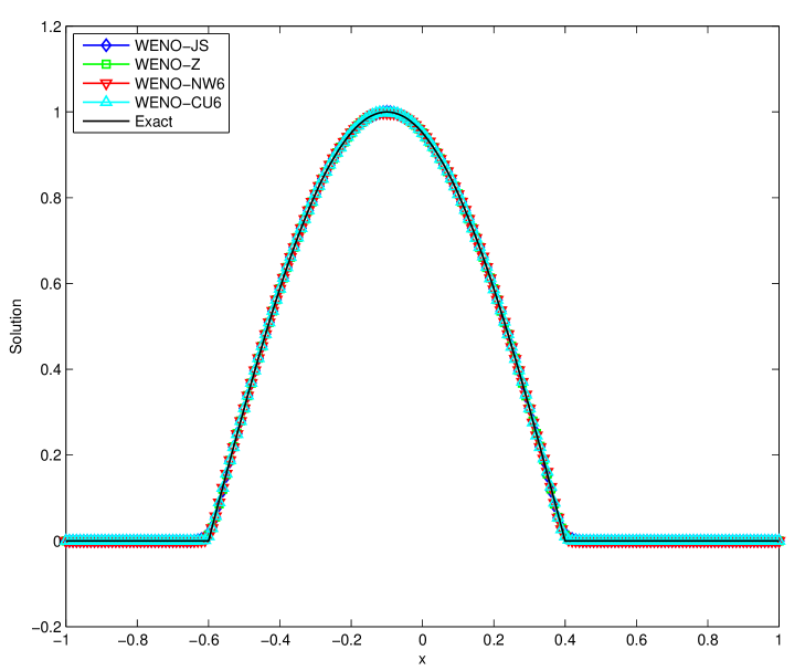
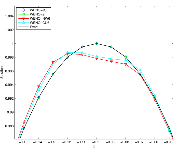
Figure 1. Left: Numerical solutions of Eq. (1.2) at time $t=2.4$ obtained from different WENO schemes. Right: Zoom near the critical region.

Our goal in this work is to construct a new WENO scheme which overcomes the drawback of WENO-NW6 and WENO-CU6 presented in the previous example. For this, we introduce a different switching mechanism between a 5th-order upwind and 6th-order central scheme. Unlike the WENO-NW6 or WENO-CU6 scheme in which the change depends on the smoothness indicator of the most downwind sub-stencil, in our scheme, whether the scheme is upwind or central is due to the smoothness indicator of the large stencil. Moreover, instead of using all six points for the indicator $\beta_{3}$, we reduce the number of points down to only four. The reason for this is explained in the below section. We also introduce a new set of smoothness indicators which are constructed in a central sense in Taylor expansions with respect to the point $x_{j}$. The feature of our new scheme is that it automatically switches between a 5th-order upwind scheme near discontinuities to prevent spurious oscillations, and a 6th-order central scheme in smooth regions which improves the loss of accuracy of the WENO-NW6 and WENO-CU6 schemes. Moreover, it is shown in the numerical results below that the new scheme maintains symmetry in the solutions much better than the 6th-order ones.

We organize our paper as follows. In section 2, we summarize the mentioned above WENO schemes which relate to our work. From there, we construct our new scheme in section 3. In this section, we first start with the new definition of the central smoothness indicators. We then introduce a new switching mechanism for 5th-order upwind and 6th-order central scheme. Numerical results comparing the performances of all schemes are presented in section 4. Finally, we close our discussions with a conclusion section.

2. Summary on Finite Difference WENO Schemes

For simplicity, we consider Eq. (1.1) in a scalar case. We rewrite the equation as follows,

(2.1) $$\begin{cases}&u_{t}+f(u)_{x}=0,\quad x\in[x_{l},x_{r}],\\ &u(x,0)=u_{0}(x).\end{cases}$$

We first define a uniformly spatial grid $x_{j}=x_{l}+j\Delta x$, $j=0,\ldots,N$, where $\Delta x$ is the grid size. We denote the interval $I_{j}=[x_{j-\frac{1}{2}},x_{j+\frac{1}{2}}]$ where $x_{j\pm\frac{1}{2}}=x_{j}\pm\frac{\Delta x}{2}$ are the interfaces of $I_{j}$. We also denote all quantities with a subscript $(\cdot)_{j}$ their grid values at $x_{j}$, for examples, $u_{j}=u(x_{j},\cdot)$, $f_{j}=f(u_{j})$, etc.; and so as with a subscript $(\cdot)_{j+\frac{1}{2}}$ for the quantities at the interface $x_{j+\frac{1}{2}}$. Whether these quantities are exact or approximate depends on particular circumstances.

We denote $h(x)$ the numerical flux function defined as follows,

(2.2) $$f(u(x,\cdot))=\bar{h}(x):=\dfrac{1}{\Delta x}\int_{x-\frac{\Delta x}{2}}^{x+\frac{\Delta x}{2}}h(y)dy.$$

Evaluating Eq. (2.1) at grid point $x_{j}$, we obtain the semi-discretized form as follows,

(2.3) $$\dfrac{du_{j}}{dt}=-\dfrac{\partial f}{\partial x}\bigg{|}_{x=x_{j}}=-\dfrac{h(x_{j+\frac{1}{2}})-h(x_{j-\frac{1}{2}})}{\Delta x}=:\mathcal{L}(u).$$

It is noticed that Eq. (2.3) is exact since there are no approximating errors in the formula.

2.1. Time Integration

We first mention about time advancing for Eq. (2.3). Following [GS98] and the references therein, for all below WENO schemes, we employ the 3rd-order TVD Runge-Kutta method as below. For TVD, we mean that the time integrator follows the same property mentioned above. Here, $\Delta t$ is the time step satisfying some proper CFL condition.

(2.4) $$\begin{split}&u^{(1)}=u^{n}+\Delta t\hat{\mathcal{L}}(u^{n}),\\ &u^{(2)}=\dfrac{3}{4}u^{n}+\dfrac{1}{4}u^{(1)}+\dfrac{1}{4}\Delta t\hat{\mathcal{L}}(u^{(1)}),\\ &u^{n+1}=\dfrac{1}{3}u^{n}+\dfrac{2}{3}u^{(2)}+\dfrac{2}{3}\Delta t\hat{\mathcal{L}}(u^{(2)}),\end{split}$$

where $\hat{\mathcal{L}}(u)$ obtained from some method is an approximation of the spatial operator $\mathcal{L}(u)$. In particular, see the below WENO discretizations $\hat{\mathcal{L}}^{5}(u)$ in Eq. (2.12) where $\hat{f}^{5}_{j+\frac{1}{2}}=\hat{f}_{j+\frac{1}{2}}$ follows Eq. (2.13) and $\hat{\mathcal{L}}^{6}(u)$ in Eq. (2.46) where $\hat{f}^{6}_{j+\frac{1}{2}}$ is defined in Eq. (2.47) with $\gamma_{k}$’s replaced by $\omega_{k}$’s.

We now proceed to the discussions on the spatial discretizations.

2.2. 5th-order Upwind WENO Reconstruction

We notice that for simplicity, we can assume that $f^{\prime}(u)\geq 0$ over the whole computational domain. In case there is a change in signs of $f^{\prime}(u)$, a flux splitting technique is invoked. We discuss this in Remark 2.1 below.

Originally, WENO schemes were constructed in the context of finite volume (see [LOC94]). Thanks to Lemma $3.1$ given in [Sh09], the schemes can be transformed into finite difference through relation (2.2). The $\bar{h}_{j}$ is called an average value of the numerical flux $h(x)$ over the interval $I_{j}$. We then seek for an approximating polynomial $\hat{f}^{5}(x)$ of degree four of $h(x)$ as below

(2.5) $$h(x)\approx\hat{f}^{5}(x)=a_{0}+a_{1}x+a_{2}x^{2}+a_{3}x^{3}+a_{4}x^{4},$$

over the large stencil $S^{5}=\{x_{j-2},x_{j-1},x_{j},x_{j+1},x_{j+2}\}$. We note that $S^{5}$ is chosen biased to the left with respect to the point $x_{j+\frac{1}{2}}$ for the stability purpose. Hence, the scheme is in an upwind sense.

Replacing the integrand $h(x)$ in Eq. (2.2) by its approximation $\hat{f}^{5}(x)$ in Eq. (2.5) and evaluating at $x_{k}$, $k=j-2,\ldots,j+2$, we can uniquely determine the coefficients $a_{k}$’s, $k=0,\ldots,4$. Since the procedure is via the average $\bar{h}_{k}=\bar{h}(x_{k})=f(u(x_{k},\cdot))$ in Eq. (2.2), it is called reconstruction and $\hat{f}^{5}(x)$ is the reconstruction polynomial. Evaluating $\hat{f}^{5}(x)$ at $x_{j+\frac{1}{2}}$, we obtain the approximation of $h_{j+\frac{1}{2}}$ as follows,

(2.6) $$\hat{f}^{5}_{j+\frac{1}{2}}=\dfrac{2}{60}f_{j-2}-\dfrac{13}{60}f_{j-1}+\dfrac{47}{60}f_{j}+\dfrac{27}{60}f_{j+1}-\dfrac{3}{60}f_{j+2}.$$

Here, we recall $f_{k}=f(u_{k})=f(u(x_{k},\cdot))$.

To justify the approximation error, we denote the polynomial $H(x)$ such that

(2.7) $$H^{\prime}(x)=h(x).$$

We then deduce from Eq. (2.2) that

(2.8) $$f(u(x,\cdot))=\dfrac{1}{\Delta x}\int_{x-\frac{\Delta x}{2}}^{x+\frac{\Delta x}{2}}H^{\prime}(y)dy=\dfrac{H(x+\frac{\Delta x}{2})-H(x-\frac{\Delta x}{2})}{\Delta x}.$$

Substituting Eq. (2.8) into the approximation (2.6), evaluating at $x_{k}$, $k=j-2,\ldots,j+2$, and applying Taylor expansions of $H(x)$ at $x=x_{j+\frac{1}{2}}$, we obtain the following truncation error,

(2.9) $$\begin{split}\hat{f}^{5}_{j+\frac{1}{2}}&=\dfrac{1}{60\Delta x}(-2H_{j-\frac{5}{2}}+15H_{j-\frac{3}{2}}-60H_{j-\frac{1}{2}}+20H_{j+\frac{1}{2}}+30H_{j+\frac{3}{2}}-3H_{j+\frac{5}{2}})\\ &=H^{\prime}_{j+\frac{1}{2}}-\dfrac{1}{60}\dfrac{d^{6}H}{dx^{6}}\bigg{|}_{x=x_{j+\frac{1}{2}}}\Delta x^{5}+\mathcal{O}(\Delta x^{6})=h_{j+\frac{1}{2}}-\dfrac{1}{60}\dfrac{\partial^{5}f}{\partial x^{5}}\bigg{|}_{x=x_{j}}\Delta x^{5}+\mathcal{O}(\Delta x^{6}).\end{split}$$

The last equality in Eq. (2.9) is justified as follows. Thanks to the relation in (2.8), by a Taylor expansion around $x_{j+\frac{1}{2}}$ we have that

(2.10) $$\begin{split}\dfrac{\partial^{5}f}{\partial x^{5}}\bigg{|}_{x=x_{j}}&=\dfrac{1}{\Delta x}\left[\dfrac{d^{5}H}{dx^{5}}\bigg{|}_{x=x_{j+\frac{1}{2}}}-\dfrac{d^{5}H}{dx^{5}}\bigg{|}_{x=x_{j+\frac{1}{2}}-\Delta x}\right]=\dfrac{d^{6}H}{dx^{6}}\bigg{|}_{x=x_{j+\frac{1}{2}}}+\mathcal{O}(\Delta x).\end{split}$$

Together with Eq. (2.7), we deduce the last equality in Eq. (2.9).

Similarly, we have

(2.11) $$\hat{f}^{5}_{j-\frac{1}{2}} =\dfrac{2}{60}f_{j-3}-\dfrac{13}{60}f_{j-2}+\dfrac{47}{60}f_{j-1}+\dfrac{27}{60}f_{j}-\dfrac{3}{60}f_{j+1}$$

$$=h_{j-\frac{1}{2}}-\dfrac{1}{60}\dfrac{\partial^{5}f}{\partial x^{5}}\bigg{|}_{x=x_{j}}\Delta x^{5}+\mathcal{O}(\Delta x^{6}).$$

Hence, we have

(2.12) $$\dfrac{du_{j}}{dt}\approx-\dfrac{\hat{f}^{5}_{j+\frac{1}{2}}-\hat{f}^{5}_{j-\frac{1}{2}}}{\Delta x}=:\hat{\mathcal{L}}^{5}(u).$$

The scheme is 5th-order of accuracy in space.

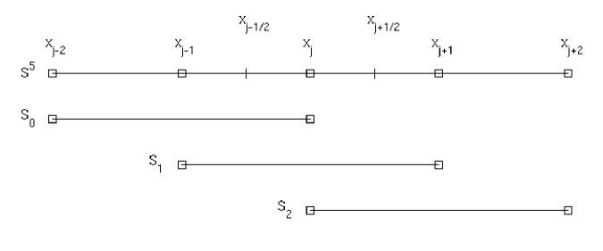
Figure 2. Stencils for 5th-order WENO schemes.

For non-smooth solutions, we employ WENO reconstruction. The idea of WENO schemes is that, instead of the 5-point stencil $S^{5}$, a convex combination of three 3-point sub-stencils are facilitated for an adaptive choice of candidates for the reconstruction. That is,

(2.13) $$\hat{f}_{j+\frac{1}{2}}=\sum_{k=0}^{2}\omega_{k}\hat{f}^{k}_{j+\frac{1}{2}},$$

where $\hat{f}^{k}_{j+\frac{1}{2}}$’s are defined below and $\omega_{k}$ is the non-linear weight satisfying $\omega_{k}\geq 0,\ \forall k$ and

(2.14) $$\sum_{k=0}^{2}\omega_{k}=1.$$

The necessity of non-negative nonlinear weights is discussed in [LSZ09] and in [SHS02] for practical implementations. And $\hat{f}^{k}_{j+\frac{1}{2}}$ is the approximation of $h_{j+\frac{1}{2}}$ by the reconstruction polynomial $\hat{f}^{k}(x)=b_{0}+b_{1}x+b_{2}x^{2}$ over the sub-stencil $S_{k}$, $k=0,1,2$. Here, $S_{0}=\{x_{j-2},x_{j-1},x_{j}\}$, $S_{1}=\{x_{j-1},x_{j},x_{j+1}\}$, and $S_{2}=\{x_{j},x_{j+1},x_{j+2}\}$ (see Fig. 2). Carrying a similar process as for the large stencil $S^{5}$, we find that around $x_{j}=0$,

(2.15) $$\hat{f}^{0}(x)=\dfrac{-f_{j-2}+2f_{j-1}+23f_{j}}{24}+\left(\dfrac{f_{j-2}-4f_{j-1}+3f_{j}}{2\Delta x}\right)x+\left(\dfrac{f_{j-2}-2f_{j-1}+f_{j}}{2\Delta x^{2}}\right)x^{2},$$

(2.16) $$\hat{f}^{1}(x)=\dfrac{-f_{j-1}+26f_{j}-f_{j+1}}{24}+\left(\dfrac{f_{j+1}-f_{j-1}}{2\Delta x}\right)x+\left(\dfrac{f_{j-1}-2f_{j}+f_{j+1}}{2\Delta x^{2}}\right)x^{2},$$

(2.17) $$\hat{f}^{2}(x)=\dfrac{23f_{j}+2f_{j+1}-f_{j+2}}{24}+\left(\dfrac{-3f_{j}+4f_{j+1}-f_{j+2}}{2\Delta x}\right)x+\left(\dfrac{f_{j}-2f_{j+1}+f_{j+2}}{2\Delta x^{2}}\right)x^{2}.$$

Evaluating each of these $\hat{f}^{k}(x)$’s at $x_{j+\frac{1}{2}}$, we obtain that

(2.18) $$\hat{f}^{0}_{j+\frac{1}{2}}=\dfrac{2}{6}f_{j-2}-\dfrac{7}{6}f_{j-1}+\dfrac{11}{6}f_{j},$$

(2.19) $$\hat{f}^{1}_{j+\frac{1}{2}}=-\dfrac{1}{6}f_{j-1}+\dfrac{5}{6}f_{j}+\dfrac{2}{6}f_{j+1},$$

(2.20) $$\hat{f}^{2}_{j+\frac{1}{2}}=\dfrac{2}{6}f_{j}+\dfrac{5}{6}f_{j+1}-\dfrac{1}{6}f_{j+2}.$$

Carrying a similar process as given in Eqs. (2.9) - (2.10) with $\hat{f}^{k}_{j+\frac{1}{2}}$ replacing $\hat{f}^{5}_{j+\frac{1}{2}}$, we obtain that

(2.21) $$h_{j+\frac{1}{2}}=\hat{f}^{k}_{j+\frac{1}{2}}+\mathcal{O}(\Delta x^{3}).$$

Comparing between $\hat{f}^{5}_{j+\frac{1}{2}}$ given in Eq. (2.6) and the ones in Eqs. (2.18) - (2.20), we deduce the following linear relation

(2.22) $$\hat{f}^{5}_{j+\frac{1}{2}}=\sum_{k=0}^{2}\gamma_{k}\hat{f}^{k}_{j+\frac{1}{2}},$$

where

(2.23) $$\gamma_{0}=\frac{1}{10},\quad\gamma_{1}=\frac{6}{10},\quad\gamma_{2}=\frac{3}{10},$$

are called the linear (optimal) weights. We note that

(2.24) $$\sum_{k=0}^{2}\gamma_{k}=1.$$

Adding and subtracting $\sum_{k=0}^{2}\gamma_{k}\hat{f}^{k}_{j+\frac{1}{2}}$ into and from Eq. (2.13), thanks to the truncation errors in Eqs. (2.9), (2.21), the normalization in Eqs. (2.14), (2.24), and the linear relation (2.22) we obtain that

(2.25) $$\begin{split}\hat{f}_{j\pm\frac{1}{2}}&=\sum_{k=0}^{2}(\omega^{\pm}_{k}-\gamma^{\pm}_{k})\hat{f}^{k}_{j^{\pm}\frac{1}{2}}+\sum_{k=0}^{2}\gamma^{\pm}_{k}\hat{f}^{k}_{j^{\pm}\frac{1}{2}}\\ &=\sum_{k=0}^{2}(\omega^{\pm}_{k}-\gamma^{\pm}_{k})(h_{j^{\pm}\frac{1}{2}}+\mathcal{O}(\Delta x^{3}))+\left(h_{j^{\pm}\frac{1}{2}}-\dfrac{1}{60}\dfrac{\partial^{5}f}{\partial x^{5}}\bigg{|}_{x=x_{j}}\Delta x^{5}+\mathcal{O}(\Delta x^{6})\right)\\ &=h_{j^{\pm}\frac{1}{2}}-\dfrac{1}{60}\dfrac{\partial^{5}f}{\partial x^{5}}\bigg{|}_{x=x_{j}}\Delta x^{5}+\sum_{k=0}^{2}(\omega^{\pm}_{k}-\gamma^{\pm}_{k})\mathcal{O}(\Delta x^{3})+\mathcal{O}(\Delta x^{6}),\end{split}$$

where $\gamma^{\pm}_{k}$, $\omega^{\pm}_{k}$ are the linear and non-linear weights of the sub-stencils $S^{j\pm\frac{1}{2}}_{k}$ corresponding to the interfaces $x_{j\pm\frac{1}{2}}$, respectively.

Hence, in order that the discretization in Eq. (2.12) where $\hat{f}^{5}_{j\pm\frac{1}{2}}=\hat{f}_{j\pm\frac{1}{2}}$ follow the nonlinear relation (2.13) to be 5th-order, we deduce the sufficient condition for the nonlinear weights as follows,

(2.26) $$\omega^{\pm}_{k}-\gamma^{\pm}_{k}=\mathcal{O}(\Delta x^{3}),\quad\forall k.$$

Different WENO schemes depends on how these nonlinear weights and the smoothness indicators are defined. The latter ones are introduced in the below section. In the following subsections, we summarize the 5th-order upwind and 6th-order central WENO schemes discussed previously. Since WENO-Z is a good replacement for WENO-M, we omit the latter one in our comparison.

2.2.1. WENO-JS

In [JS96], Jiang and Shu defined the nonlinear weights as follows,

(2.27) $$\omega^{JS}_{k}=\dfrac{\alpha^{JS}_{k}}{\sum_{l=0}^{2}\alpha^{JS}_{l}},\quad\alpha^{JS}_{k}=\dfrac{\gamma_{k}}{(\varepsilon+\beta_{k})^{p}},$$

where $\gamma_{k}$ is defined in Eq. (2.23), $\beta_{k}$ is called the smoothness indicator of $S_{k}$ which measures how smooth the solution is over this sub-stencil. The authors defined these $\beta_{k}$’s through the normalized $L^{2}$-norm of high-order variations of the reconstruction polynomials given in Eqs. (2.18) - (2.20). Explicitly, for a 5th-order scheme, we have

(2.28) $$\beta_{k}=\Delta x\int_{x_{j-\frac{1}{2}}}^{x_{j+\frac{1}{2}}}\left(\dfrac{d}{dx}\hat{f}^{k}(x)\right)^{2}dx+\Delta x^{3}\int_{x_{j-\frac{1}{2}}}^{x_{j+\frac{1}{2}}}\left(\dfrac{d^{2}}{dx^{2}}\hat{f}^{k}(x)\right)^{2}dx,$$

where $\hat{f}^{k}(x)$’s are as in Eqs. (2.15) - (2.17) and the sub-stencils $S_{0}$, $S_{1}$, $S_{2}$ are centered around $x_{j}=0$.

Evaluating for each $k$, we obtain that

(2.29) $$\beta_{0} =\frac{13}{12}(f_{j-2}-2f_{j-1}+f_{j})^{2}+\frac{1}{4}(f_{j-2}-4f_{j-1}+3f_{j})^{2}$$

$$=f^{\prime 2}\Delta x^{2}+\left(\frac{13}{12}f^{\prime\prime 2}-\frac{2}{3}f^{\prime}f^{\prime\prime\prime}\right)\Delta x^{4}+\mathcal{O}(\Delta x^{5}),$$

(2.30) $$\beta_{1} =\frac{13}{12}(f_{j-1}-2f_{j}+f_{j+1})^{2}+\frac{1}{4}(f_{j+1}-f_{j-1})^{2}$$

$$=f^{\prime 2}\Delta x^{2}+\left(\frac{13}{12}f^{\prime\prime 2}+\frac{1}{3}f^{\prime}f^{\prime\prime\prime}\right)\Delta x^{4}+\mathcal{O}(\Delta x^{6}),$$

(2.31) $$\beta_{2} =\frac{13}{12}(f_{j}-2f_{j+1}+f_{j+2})^{2}+\frac{1}{4}(3f_{j}-4f_{j+1}+f_{j+2})^{2}$$

$$=f^{\prime 2}\Delta x^{2}+\left(\frac{13}{12}f^{\prime\prime 2}-\frac{2}{3}f^{\prime}f^{\prime\prime\prime}\right)\Delta x^{4}+\mathcal{O}(\Delta x^{5}),$$

where the derivatives are evaluated at $x=x_{j}$.

In formula (2.27), $\varepsilon$ is a small parameter to prevent division by zero. In most cases, WENO-JS works well with $\varepsilon=10^{-6}$. A thorough analysis of the role of $\varepsilon$ can be found in [HAP05]. The parameter $p$ is to increase the dissipation of the scheme. For WENO-JS, $p=2$ is chosen.

If $f^{\prime}_{j}=f^{\prime}(x_{j})\neq 0$, $\forall k$, $\beta_{k}$ can be written in the form

(2.32) $$\beta_{k}=(f^{\prime}_{j}\Delta x)^{2}(1+\mathcal{O}(\Delta x^{2})).$$

Substituting these into Eq. (2.27) with the removal of $\varepsilon$, since $(1+y)^{-2}=1+\mathcal{O}(y)$, by Eq. (2.24) we obtain that

(2.33) $$\begin{split}\omega^{JS}_{k}=\dfrac{\gamma_{k}(f^{\prime}_{j}\Delta x)^{-2}(1+\mathcal{O}(\Delta x^{2}))}{(f^{\prime}_{j}\Delta x)^{-2}\sum_{l=0}^{2}\gamma_{l}(1+\mathcal{O}(\Delta x^{2}))}=\gamma_{k}+\mathcal{O}(\Delta x^{2}),\end{split}$$

which is a relaxed form of (2.26). We notice that for WENO-JS, $\omega^{JS}_{k}$ cannot satisfy condition (2.26) directly. Moreover, if $f^{\prime}_{j}=0$, it is observed from Eqs. (2.29) - (2.31) that $\beta_{k}=\frac{13}{12}(f^{\prime\prime}_{j})^{2}\Delta x^{4}(1+\mathcal{O}(\Delta x))$ for $k=0,2$ and $\beta_{1}=\frac{13}{12}(f^{\prime\prime}_{j})^{2}\Delta x^{4}(1+\mathcal{O}(\Delta x^{2}))$, in which the condition (2.32) is not satisfied for all $k$’s. Similarly, we find that

(2.34) $$\omega^{JS}_{k}=\gamma_{k}+\mathcal{O}(\Delta x),$$

which is a loss of accuracy near this critical point. This accuracy loss is improved by the WENO-Z scheme which is summarized in the next subsection.

2.2.2. WENO-Z

Borges et al. in [BCCD08] proposed a new WENO-Z. In their scheme, the nonlinear weights are defined differently from those of WENO-JS. They are as follows,

(2.35) $$\omega^{Z}_{k}=\dfrac{\alpha^{Z}_{k}}{\sum_{l=0}^{2}\alpha^{Z}_{l}},\quad\alpha^{Z}_{k}=\gamma_{k}\left(1+\left(\dfrac{\tau^{Z}}{\varepsilon+\beta_{k}}\right)^{q}\right),$$

where the smoothness indicators $\beta_{k}$’s are the same as those given in Eqs. (2.29) - (2.31), $\varepsilon=10^{-40}$, and $\tau^{Z}$ is the smoothness indicator of the large stencil $S^{5}$. The power $q$ is used to tune the relation between the dispersive and dissipative property of the scheme. It is checked numerically in [BCCD08] that the scheme becomes more dissipative when $q$ is increased. For WENO-Z, $\tau^{Z}$ is defined as follows,

(2.36) $$\tau^{Z}=|\beta_{0}-\beta_{2}|=\frac{13}{3}|f^{\prime\prime}f^{\prime\prime\prime}|\Delta x^{5}+\mathcal{O}(\Delta x^{6}).$$

We note that if $f^{\prime}_{j}\neq 0$ and $q=1$, $\beta_{k}=\mathcal{O}(\Delta x^{2})$, $\forall k$. Then

(2.37) $$\dfrac{\tau^{Z}}{\beta_{k}}=\mathcal{O}(\Delta x^{3}),\quad\forall k.$$

Similarly to Eq. (2.33), we obtain that

(2.38) $$\omega^{Z}_{k}=\gamma_{k}+\mathcal{O}(\Delta x^{3}),$$

directly without using the relaxed version as the WENO-JS scheme. It was also proven in [BCCD08] that WENO-Z is 4th-order near simple smooth critical points (i.e. where $f^{\prime}_{j}=0$) for $q=1$ and attains the designed 5th-order for $q=2$. The tradeoff for the latter case is that the scheme is more dissipative. Throughout this work, we choose $q=1$. One more advantage of WENO-Z over WENO-JS is that the former is more central in a sense that the stencil over which the solution is discontinuous plays more roles in the approximation of the numerical flux. This assessment is checked as follows. We suppose that $S_{2}$ contains a discontinuity whereas the solution is smooth over the other two sub-stencils. Hence, $\tau^{Z}=\mathcal{O}(1)$, $\beta_{2}=\mathcal{O}(1)$, and $\beta_{k}=\mathcal{O}(\Delta x^{2})$, $k=0,1$. Then,

(2.39) $$\begin{split}\dfrac{\alpha^{Z}_{2}}{\alpha^{Z}_{k}}=\dfrac{\gamma_{2}\left(1+\frac{\tau^{Z}}{\beta_{2}}\right)}{\gamma_{k}\left(1+\frac{\tau^{Z}}{\beta_{k}}\right)}=\dfrac{\frac{\gamma_{2}}{\beta_{2}}(\beta_{2}+\tau^{Z})}{\frac{\gamma_{k}}{\beta_{k}}(\beta_{k}+\tau^{Z})}=\dfrac{\alpha^{JS}_{2}(\beta_{2}+\tau^{Z})}{\alpha^{JS}_{k}(\beta_{k}+\tau^{Z})}\geq\dfrac{\alpha^{JS}_{2}}{\alpha^{JS}_{k}},\end{split}$$

since

(2.40) $$\dfrac{\beta_{2}+\tau^{Z}}{\beta_{k}+\tau^{Z}}\approx\dfrac{\beta_{2}+\tau^{Z}}{\tau^{Z}}\geq 1.$$

Hence, WENO-Z has a sharper capturing of discontinuities than WENO-JS.

Remark 2.1.

2. In case the condition $f^{\prime}(u)\geq 0$ is not satisfied, which is general in real applications, we apply a flux splitting technique to decompose $f(u)$ into positive and negative components. In most applications, the global Lax-Friedrichs flux splitting is used (see [JS96] and the references therein),

   (2.41) $$f^{\pm}(u)=\dfrac{1}{2}(f(u)\pm\alpha u),$$

   where $\alpha=\max|f^{\prime}(u)|$ over the whole computational domain. Then,

   (2.42) $$\hat{f}_{j+\frac{1}{2}}=\hat{f}^{+}_{j+\frac{1}{2}}+\hat{f}^{-}_{j+\frac{1}{2}}.$$

   The negative flux $\hat{f}^{-}_{j+\frac{1}{2}}$ is symmetric to $\hat{f}^{+}_{j+\frac{1}{2}}$ with respect to $x_{j+\frac{1}{2}}$.

3. If the flux splitting is employed, the overall number of grid points used in the reconstruction of the numerical flux is increased by one. That is, let $S^{5+}$ and $S^{5-}$ be the stencils over which $\hat{f}^{+}_{j+\frac{1}{2}}$ and $\hat{f}^{-}_{j+\frac{1}{2}}$ are determined, then

   (2.43) $$S^{6}:=S^{5+}\bigcup S^{5-}=\{x_{j-2},x_{j-1},x_{j},x_{j+1},x_{j+2},x_{j+3}\},$$

   which consists of six points. We note that with this $S^{6}$, there exists a polynomial of degree five which reconstructs $h(x)$ over the stencil. Therefore, the accuracy of WENO schemes can be increased up to sixth. These schemes are discussed in the subsection below.

2.3. 6th-order Central WENO Reconstruction

Carrying a similar procedure as described in the previous subsection for the 6-point large stencil $S^{6}$, we can deduce that

(2.44) $$\begin{split}\hat{f}^{6}_{j+\frac{1}{2}}&=\dfrac{1}{60}f_{j-2}-\dfrac{8}{60}f_{j-1}+\dfrac{37}{60}f_{j}+\dfrac{37}{60}f_{j+1}-\dfrac{8}{60}f_{j+2}+\dfrac{1}{60}f_{j+3}\\ &=h_{j+\frac{1}{2}}+\dfrac{1}{140}\dfrac{\partial^{6}f}{\partial x^{6}}\bigg{|}_{x=x_{j}}\Delta x^{6}+\mathcal{O}(\Delta x^{7}).\end{split}$$

Similarly,

(2.45) $$\begin{split}\hat{f}^{6}_{j-\frac{1}{2}}&=\dfrac{1}{60}f_{j-3}-\dfrac{8}{60}f_{j-2}+\dfrac{37}{60}f_{j-1}+\dfrac{37}{60}f_{j}-\dfrac{8}{60}f_{j+1}+\dfrac{1}{60}f_{j+2}\\ &=h_{j-\frac{1}{2}}+\dfrac{1}{140}\dfrac{\partial^{6}f}{\partial x^{6}}\bigg{|}_{x=x_{j}}\Delta x^{6}+\mathcal{O}(\Delta x^{7}).\end{split}$$

Hence we obtain that

(2.46) $$\dfrac{du_{j}}{dt}\approx-\dfrac{\hat{f}^{6}_{j+\frac{1}{2}}-\hat{f}^{6}_{j-\frac{1}{2}}}{\Delta x}=:\hat{\mathcal{L}}^{6}(u).$$

The scheme is increased to 6th-order of accuracy in space.

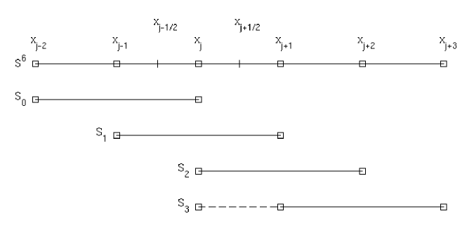
Figure 3. Stencils for 6th-order WENO schemes.

Adding one more sub-stencil $S_{3}=\{x_{j+1},x_{j+2},x_{j+3}\}$ into the approximation of the interfaced value $\hat{f}_{j+\frac{1}{2}}$ (see Fig. 3), we deduce a similar linear relation with Eq. (2.22) as follows

(2.47) $$\hat{f}^{6}_{j+\frac{1}{2}}=\sum_{k=0}^{3}\gamma_{k}\hat{f}^{k}_{j+\frac{1}{2}},$$

where

(2.48) $$\gamma_{0}=\gamma_{3}=\dfrac{1}{20},\quad\gamma_{1}=\gamma_{2}=\dfrac{9}{20}.$$

Here, $\hat{f}^{3}_{j+\frac{1}{2}}$ is the 3rd-order approximation of the numerical flux $h(x)$ at the interface $x_{j+\frac{1}{2}}$ from the reconstruction polynomial $\hat{f}^{3}(x)$ over the sub-stencil $S_{3}$. Explicitly, we have

(2.49) $$\hat{f}^{3}_{j+\frac{1}{2}}=\dfrac{11}{6}f_{j+1}-\dfrac{7}{6}f_{j+2}+\dfrac{2}{6}f_{j+3}.$$

The other approximations $\hat{f}^{k}_{j+\frac{1}{2}}$’s, $k=0,1,2$ follow Eqs. (2.18) - (2.20).

The nonlinear combination using the nonlinear weights is similar to that of the linear case (2.47), except for the linear weight $\gamma_{k}$ replaced by its nonlinear version $\omega_{k}$, $k=0,\ldots,3$.

Remark 2.2.

2. Since the accuracy order is increased to sixth, the sufficient condition for the nonlinear weights given in (2.26) is also increased by one. That is,

   (2.50) $$\omega^{\pm}_{k}-\gamma^{\pm}_{k}=\mathcal{O}(\Delta x^{4}),\ \forall k.$$

3. Observing from Eq. (2.47) that the approximations $\hat{f}_{j+\frac{1}{2}}$’s are now symmetric with respect to $x_{j+\frac{1}{2}}$. It means that the scheme now is central. Hence, spurious oscillations are expected to occur near discontinuities. A treatment on the most downwind sub-stencil $S_{3}$ is needed to sustain the essentially non-oscillatory property of the scheme. We now overview the 6th-order WENO schemes for this case.

2.3.1. WENO-NW6

In [YC09], Yamaleev and Carpenter proposed a 6th-order energy-stable WENO scheme. They introduced an artificial dissipative term and proved that this makes the new scheme be stable in $L^{2}$ sense. In this work, we only discuss their treatment on the nonlinear weights and omit this artificial dissipative term (see [YC09] for a detailed discussion on the term). Hence, the scheme here is denoted by WENO-NW6, not ESWENO as in their paper.

The nonlinear weights (denoted $\omega_{k}^{NW}$, $\alpha_{k}^{NW}$) follow those defined in the WENO-Z scheme which are given in Eq. (2.35), for $k=0,\ldots,3$. The differences lie on the smoothness indicator of the most downwind sub-stencil $\beta_{3}$ and the one for the large stencil $S^{6}$. For the former, in order that there are no oscillations occurring near discontinuities, all grid values of the flux over $S^{6}$ are accounted for the computation of $\beta_{3}$. It is as follows,

(2.51) $$\beta_{3}=\dfrac{1}{4}(\beta_{0}^{4}+\beta_{1}^{4}+\beta_{2}^{4}+\tilde{\beta}_{3}^{4})^{1/4},$$

where $\tilde{\beta}_{3}$ is computed using the formula given in Eq. (2.28). That is,

(2.52) $$\begin{split}\tilde{\beta}_{3}&=\dfrac{13}{12}(f_{j+1}-2f_{j+2}+f_{j+3})^{2}+\dfrac{1}{4}(-5f_{j+1}+8f_{j+2}-3f_{j+3})^{2}\\ &=f^{\prime 2}\Delta x^{2}+\left(\frac{13}{12}f^{\prime\prime 2}-\frac{11}{3}f^{\prime}f^{\prime\prime\prime}\right)\Delta x^{4}+\mathcal{O}(\Delta x^{5}),\end{split}$$

where the derivatives are evaluated at $x=x_{j}$. The other indicators $\beta_{k}$’s, $k=0,1,2$ follow Eqs. (2.29) - (2.31).

The smoothness indicator of the large stencil $S^{6}$ is defined as the highest, i.e., fifth-degree, undivided difference as follows

(2.53) $$\begin{split}\tau^{NW}&=(f_{j-2}-5f_{j-1}+10f_{j}-10f_{j+1}+5f_{j+2}-f_{j+3})^{2}\\ &=(f^{(5)})^{2}\Delta x^{10}+\mathcal{O}(\Delta x^{11}).\end{split}$$

Carrying a similar procedure as in Eqs. (2.37) - (2.38) with a change in $\tau$, thanks to Eq. (2.53), we obtain that

(2.54) $$\dfrac{\tau^{NW}}{\beta_{k}}=\begin{cases}&\mathcal{O}(\Delta x^{8}),\quad\text{if }f^{\prime}_{j}\neq 0,\\ &\mathcal{O}(\Delta x^{6}),\quad\text{if }f^{\prime}_{j}=0,\end{cases}\quad\forall k,$$

thus condition (2.50) is satisfied. Hence, the scheme is 6th-order in smooth regions. The case where the derivatives of $f$ vanish will be checked numerically in the below section.

2.3.2. WENO-CU6

In [HWA10], Hu et al. developed the adaptive central-upwind scheme WENO-CU6 based on the principle that the most downwind sub-stencil only plays roles in smooth regions and is suppressed near discontinuities. Hence the scheme is central in smooth regions and upwind near discontinuities. The scheme is different from WENO-NW6 in defining the smoothness indicators $\beta_{3}$ and $\tau$. In particular, they are as below,

(2.55) $$\begin{split}\beta_{3}&=\dfrac{1}{120960}[271779f_{j-2}^{2}+f_{j-2}(-2380800f_{j-1}+4086352f_{j}-3462252f_{j+1}+1458762f_{j+2}-245620f_{j+3})\\ &+f_{j-1}(5653317f_{j-1}-20427884f_{j}+17905032f_{j+1}-7727988f_{j+2}+1325006f_{j+3})+f_{j}(19510972f_{j}\\ &-35817664f_{j+1}+15929912f_{j+2}-2792660f_{j+3})+f_{j+1}(17195652f_{j+1}-15880404f_{j+2}\\ &+2863984f_{j+3})+f_{j+2}(3824847f_{j+2}-1429976f_{j+3})+139633f_{j+3}^{2}]\\ &=f^{\prime 2}\Delta x^{2}+\dfrac{13}{12}f^{\prime\prime 2}\Delta x^{4}+\mathcal{O}(\Delta x^{6}).\end{split}$$

It is noticed that there is a typo in Eq. (25) in [HWA10], and we have corrected it in Eq. (2.55).

From there, the smoothness indicator of the large stencil $S^{6}$ is defined as follows,

(2.56) $$\tau^{CU}=\beta_{3}-\dfrac{1}{6}(\beta_{0}+4\beta_{1}+\beta_{2})=\mathcal{O}(\Delta x^{6}).$$

Hence, we have for $k=0,\ldots,3,$,

(2.57) $$\dfrac{\tau^{CU}}{\beta_{k}}=\begin{cases}&\mathcal{O}(\Delta x^{4}),\quad\text{if }f^{\prime}_{j}\neq 0,\\ &\mathcal{O}(\Delta x^{2}),\quad\text{if }f^{\prime}_{j}=0,\end{cases}$$

which satisfies the condition (2.50).

It is also noteworthy that $\alpha^{CU}_{k}$ in Eq. (2.35) has a change as below,

(2.58) $$\alpha^{CU}_{k}=\gamma_{k}\left(C+\dfrac{\tau^{CU}}{\varepsilon+\beta_{k}}\right),$$

where $C\gg 1$ is to increase the contribution of the linear weights when the smoothness indicators have comparable magnitudes (see [TWM07]). Following [HWA10], we choose $C=20$.

As indicated in example 1.1, the 6th-order WENO-NW6 and WENO-CU6 schemes suffer from the loss of accuracy near the smooth critical points just right behind, with respect to the characteristic direction, a critical point where the first derivative of the solution is undefined, that is, the solution is just $C^{0}$ at that point. The explanation for this defect is given in the below section. In the next section, we propose a new scheme which automatically switches between a 6th-order central and 5th-order upwind scheme and overcomes the defect occurred in the mentioned schemes.

3. The New Scheme

We first observe that the 5th- and 6th-order linear approximations given in Eqs. (2.6) and (2.44), respectively, can be combined linearly in the following manner,

(3.1) $$\hat{f}_{j+\frac{1}{2}}=\gamma^{\theta}_{0}\hat{f}^{0}_{j+\frac{1}{2}}+\gamma^{\theta}_{1}\hat{f}^{1}_{j+\frac{1}{2}}+\gamma^{\theta}_{2}\hat{f}^{2}_{j+\frac{1}{2}}+\gamma^{\theta}_{3}\hat{f}^{3}_{j+\frac{1}{2}},$$

where

(3.2) $$\gamma^{\theta}_{0}=\frac{1}{20}(1+\theta),\quad\gamma^{\theta}_{1}=\frac{3}{20}(3+\theta),\quad\gamma^{\theta}_{2}=\frac{3}{20}(3-\theta),\quad\gamma^{\theta}_{3}=\frac{1}{20}(1-\theta),$$

and $\hat{f}^{k}_{j+\frac{1}{2}}$, $k=0,1,2,3$ is given in Eqs. (2.18) - (2.20) and (2.49), respectively.

We deduce that

(3.3) $$\hat{f}_{j+\frac{1}{2}}=\begin{cases}&\hat{f}^{5}_{j+\frac{1}{2}}\quad\text{if }\theta=1,\\ &\hat{f}^{6}_{j+\frac{1}{2}}\quad\text{if }\theta=0.\end{cases}$$

We then propose a new scheme in which $\hat{f}_{j+\frac{1}{2}}$ is chosen between $\hat{f}^{5}_{j+\frac{1}{2}}$ and $\hat{f}^{6}_{j+\frac{1}{2}}$ adaptively. Hence, the scheme is $5$th-order upwind or $6$th-order central depending on the smoothness of the stencils $S^{5}$ and $S^{6}$. We expect that this will get over the drawback of accuracy degeneration of the above mentioned central 6th-order schemes. To proceed, we first rewrite Eq. (3.1) using instead the non-linear weights $\omega^{\theta}_{k}$’s as follows,

(3.4) $$\hat{f}_{j+\frac{1}{2}}=\omega^{\theta}_{0}\hat{f}^{0}_{j+\frac{1}{2}}+\omega^{\theta}_{1}\hat{f}^{1}_{j+\frac{1}{2}}+\omega^{\theta}_{2}\hat{f}^{2}_{j+\frac{1}{2}}+\omega^{\theta}_{3}\hat{f}^{3}_{j+\frac{1}{2}},$$

where, for $k=0,\ldots,3$, and

(3.5) $$\omega^{\theta}_{k}=\dfrac{\alpha^{\theta}_{k}}{\sum_{l=0}^{3}\alpha^{\theta}_{l}},\quad\alpha^{\theta}_{k}=\gamma^{\theta}_{k}\left(1+\dfrac{\tau^{\theta}}{\varepsilon+\tilde{\beta}_{k}}\right).$$

Here, $\tau^{\theta}$ is the smoothness indicator of the large stencil, and $\tilde{\beta}_{k}$ is the smoothness indicator of the sub-stencil $S_{k}$. We define these indicators in the following subsection.

3.1. The Central Smoothness Indicators $\tilde{\beta}_{k}$ and New $\tau^{\theta}$

For a 6th-order central scheme over the large stencil $S^{6}$, spurious oscillations are expected to occur near discontinuities. To overcome this, WENO-NW6 and WENO-CU6 choose to construct their $\beta_{3}$ over all points of $S^{6}$. A more careful observation reveals that this cost can be reduced in the following way. We remind the principle of WENO schemes is that there is at least one smoothest sub-stencil is used in the reconstruction of the numerical flux. We suppose that $\beta_{3}$ follows Eq. (2.52), that is, it measures the smoothness of the most downwind $S_{3}$ only. We further assume that the grid size $\Delta x$ is so small that a discontinuity does not spread over two neighboring grid points, then for a 6th-order WENO scheme, the only case where oscillations occur is when a discontinuity is in between $x_{j}$ and $x_{j+1}$. In this case, both $\hat{f}^{0}_{j+\frac{1}{2}}$ and $\hat{f}^{3}_{j+\frac{1}{2}}$ play main roles in the combination (3.4) since $\beta_{0}$ and $\beta_{3}$ are much smaller than the other two. This leads to oscillations since the downwind $\hat{f}^{3}_{j+\frac{1}{2}}$ is wrongly chosen. To prevent this from happening, we choose $\beta_{3}$ to measure the smoothness of an extended sub-stencil $\tilde{S}_{3}:=\{x_{j},x_{j+1},x_{j+2},x_{j+3}\}$ (see Fig. 3 with $S_{3}$ extended by the dashed line). It is observed that $S_{2}$ is now a subset of $\tilde{S}_{3}$ and all sub-stencils share the point $x_{j}$. Hence, the case where oscillations occur is essentially eliminated. Moreover, the cost of computing $\beta_{3}$ is now much reduced since the computation involves only four grid points defined in $\tilde{S}_{3}$ instead of six in $S^{6}$ as in WENO-NW6 or WENO-CU6.

For 5th-order schemes, all sub-stencils are symmetric with respect to $x_{j}$. As a result, the smoothness indicators $\beta_{k}$’s are also symmetric with respect to $x_{j}$ (see Eqs. (2.29) - (2.31)). That is, $\beta_{0}$ and $\beta_{2}$ are equal to each other up to order $\mathcal{O}(\Delta x^{4})$ in Taylor expansions. We recall that WENO discretizations choose the sub-stencils depending on the non-linear weights $\omega_{k}$’s which are very sensitive to the smoothness indicators $\beta_{k}$’s due to the latter’s smallness in smooth regions (see Eq. (2.27) for WENO-JS, Eq. (2.35) for WENO-Z, WENO-NW6, and WENO-CU6). For the sensitivity, we mean that a small change in any $\beta_{k}$ leads to a large difference among $\alpha_{k}$’s, thus $\omega_{k}$’s. In that sense, the symmetry in terms of Taylor expansions of $\beta_{k}$’s reduces the effects of this sensitivity, especially in transition regions where the solution is smooth and discontinuous. We refer to Figs. 5 and 7 below for numerical evidences for this assessment in which the schemes with symmetric $\beta_{k}$’s (i.e., WENO-Z and WENO-$\theta$) show better results than the ones without this property. Unfortunately, the 6th-order methods lack of this (comparing $\beta_{3}$ in Eq. (2.51) for WENO-NW6, and Eq. (2.55) for WENO-CU6 with the other $\beta_{k}$’s, $k=0,1,2$, defined Eqs. (2.29) - (2.31)). In our new scheme, we try to recover the property. We devise our new smoothness indicators in a central sense. That is, they are constructed based on the reconstruction polynomials which are symmetric with respect to $x_{j+\frac{1}{2}}$. In addition, it is shown below that the new indicators are symmetric in terms of Taylor expansions with respect to $x_{j}$. We notice that Taylor expansions about $x_{j}$ are natural since the approximation of $f(u)_{x}$ is at the interval center $x_{j}$ (see Eq. (2.3)) although the reconstruction of the numerical flux function $h(x)$ is at the interface $x_{j+\frac{1}{2}}$ (see Eqs. (2.6) and (2.44) for 5th-order and 6th-order schemes, respectively).

Proceeding the reconstruction procedure as given in subsection 2.2, but instead around $x_{j+\frac{1}{2}}=0$ and with $\tilde{S}_{3}$ replacing $S_{3}$, we obtain that

(3.6) $$\tilde{f}^{0}(x)=\dfrac{2f_{j-2}-7f_{j-1}+11f_{j}}{6}+\left(\dfrac{f_{j-2}-3f_{j-1}+2f_{j}}{\Delta x}\right)x+\left(\dfrac{f_{j-2}-2f_{j-1}+f_{j}}{2\Delta x^{2}}\right)x^{2},$$

(3.7) $$\tilde{f}^{1}(x)=\dfrac{-f_{j-1}+5f_{j}+2f_{j+1}}{6}+\left(\dfrac{f_{j+1}-f_{j}}{\Delta x}\right)x+\left(\dfrac{f_{j-1}-2f_{j}+f_{j+1}}{2\Delta x^{2}}\right)x^{2},$$

(3.8) $$\tilde{f}^{2}(x)=\dfrac{2f_{j}+5f_{j+1}-f_{j+2}}{6}+\left(\dfrac{f_{j+1}-f_{j}}{\Delta x}\right)x+\left(\dfrac{f_{j}-2f_{j+1}+f_{j+2}}{2\Delta x^{2}}\right)x^{2},$$

(3.9) $$\begin{split}\tilde{f}^{3}(x)&=\dfrac{3f_{j}+13f_{j+1}-5f_{j+2}+f_{j+3}}{12}+\left(\dfrac{-11f_{j}+9f_{j+1}+3f_{j+2}-f_{j+3}}{12\Delta x}\right)x\\ &+\left(\dfrac{3f_{j}-7f_{j+1}+5f_{j+2}-f_{j+3}}{4\Delta x^{2}}\right)x^{2}+\left(\dfrac{-f_{j}+3f_{j+1}-3f_{j+2}+f_{j+3}}{6\Delta x^{3}}\right)x^{3}.\end{split}$$

We notice that these reconstruction polynomials are different from those given in Eqs. (2.15) - (2.17) which are constructed symmetrically with respect to $x_{j}=0$. Substituting these into Eq. (2.28) with $\tilde{f}^{k}(x)$ replacing $\hat{f}^{k}(x)$, $k=0,1,2,3$, we deduce the new central smoothness indicators as follows,

(3.10) $$\begin{split}\tilde{\beta}_{0}&=\frac{13}{12}(f_{j-2}-2f_{j-1}+f_{j})^{2}+(f_{j-2}-3f_{j-1}+2f_{j})^{2}\\ &=f^{\prime 2}\Delta x^{2}+f^{\prime}f^{\prime\prime}\Delta x^{3}+\left(\frac{4}{3}f^{\prime\prime 2}-\frac{5}{3}f^{\prime}f^{\prime\prime\prime}\right)\Delta x^{4}+\mathcal{O}(\Delta x^{5}),\end{split}$$

(3.11) $$\begin{split}\tilde{\beta}_{1}&=\frac{13}{12}(f_{j-1}-2f_{j}+f_{j+1})^{2}+(f_{j+1}-f_{j})^{2}\\ &=f^{\prime 2}\Delta x^{2}+f^{\prime}f^{\prime\prime}\Delta x^{3}+\left(\frac{4}{3}f^{\prime\prime 2}+\frac{1}{3}f^{\prime}f^{\prime\prime\prime}\right)\Delta x^{4}+\mathcal{O}(\Delta x^{5}),\end{split}$$

(3.12) $$\begin{split}\tilde{\beta}_{2}&=\frac{13}{12}(f_{j}-2f_{j+1}+f_{j+2})^{2}+(f_{j}-f_{j+1})^{2}\\ &=f^{\prime 2}\Delta x^{2}+f^{\prime}f^{\prime\prime}\Delta x^{3}+\left(\frac{4}{3}f^{\prime\prime 2}+\frac{1}{3}f^{\prime}f^{\prime\prime\prime}\right)\Delta x^{4}+\mathcal{O}(\Delta x^{5}),\end{split}$$

and

(3.13) $$\begin{split}\tilde{\beta}_{3}&=\frac{13}{48}(3f_{j}-7f_{j+1}+5f_{j+2}-f_{j+3})^{2}+(2f_{j+1}-3f_{j+2}+f_{j+3})^{2}\\ &=f^{\prime 2}\Delta x^{2}+f^{\prime}f^{\prime\prime}\Delta x^{3}+\left(\frac{4}{3}f^{\prime\prime 2}-\frac{5}{3}f^{\prime}f^{\prime\prime\prime}\right)\Delta x^{4}+\mathcal{O}(\Delta x^{5}),\end{split}$$

where the derivatives are evaluated at $x=x_{j}$. We note that for the most downwind $\tilde{\beta}_{3}$, we treated $\tilde{f}_{3}(x)$ in Eq. (3.9) as a 2nd-degree polynomial by ignoring the 3rd-degree term when substituting it into Eq. (2.28) so that $\int_{x_{j-\frac{1}{2}}}^{x_{j+\frac{1}{2}}}\left(\frac{d^{2}}{dx^{2}}\tilde{f}^{3}(x)\right)^{2}dx$ is the highest-order variation. This is for the consistency with the other reconstruction polynomials $\tilde{f}^{k}$’s, $k=0,1,2$, which are of lower-degree. We also modified the second term in the obtained indicator so that its Taylor expansion agrees with that of $\tilde{\beta}_{0}$ up to order $\mathcal{O}(\Delta x^{4})$; thus all $\tilde{\beta}_{k}$’s are now symmetric with respect to $x_{j}$ in Taylor expansions, which is our goal in designing these new smoothness indicators. The original smoothness indicator $\hat{\beta}_{3}$ for $\tilde{\beta}_{3}$ obtained from Eq. (2.28) was as below,

(3.14) $$\hat{\beta}_{3}=\frac{13}{48}(3f_{j}-7f_{j+1}+5f_{j+2}-f_{j+3})^{2}+\frac{1}{144}(-11f_{j}+9f_{j+1}+3f_{j+2}-f_{j+3})^{2}.$$

In order to enhance the dispersion of the scheme, following the approach by Taylor et al. ([TWM07]), we set a restriction on the smoothness indicators as below, for $k=0,\ldots,3$,

(3.15) $$\tilde{\beta}_{k}=\begin{cases}&0,\quad\text{if }R(\tilde{\beta})\leq\alpha_{R},\\ &\tilde{\beta}_{k},\quad\text{otherwise};\end{cases}$$

where

(3.16) $$R(\tilde{\beta})=\dfrac{\max_{k}(\tilde{\beta}_{k})}{\varepsilon+\min_{k}(\tilde{\beta}_{k})}.$$

Here, $\alpha_{R}$ is a threshold value depending on the configurations of flows. $\alpha_{R}$ is taken small for flows with the presence of shocks. For a detailed discussion, consult [TWM07].

We next devise the smoothness indicator of the large stencil $S^{6}$. Since the one proposed by Yamaleev and Carpenter in [YC09] (see Eq. (2.53)) is too dispersive and may lead to oscillations (see the evidence in [YC09]), we introduce a new smoothness indicator $\tau^{\theta}$ which is based on Eq. (2.28) but at a much higher order variations for the large stencil $S^{6}$. We consider the following $\tau$’s,

(3.17) $$\begin{split}\tau_{5}&=\Delta x^{5}\int_{x_{j-\frac{1}{2}}}^{x_{j+\frac{1}{2}}}\left(\dfrac{d^{3}}{dx^{3}}\tilde{f}^{5}(x)\right)^{2}dx+\Delta x^{7}\int_{x_{j-\frac{1}{2}}}^{x_{j+\frac{1}{2}}}\left(\dfrac{d^{4}}{dx^{4}}\tilde{f}^{5}(x)\right)^{2}dx\\ &=\dfrac{13}{12}(f_{j-2}-4f_{j-1}+6f_{j}-4f_{j+1}+f_{j+2})^{2}+(-f_{j-1}+3f_{j}-3f_{j+1}+f_{j+2})^{2}\\ &=f^{\prime\prime\prime 2}\Delta x^{6}+f^{\prime\prime\prime}f^{(4)}\Delta x^{7}+\left(\dfrac{1}{2}f^{\prime\prime\prime}f^{(5)}+\dfrac{4}{3}(f^{(4)})^{2}\right)\Delta x^{8}+\mathcal{O}(\Delta x^{9}),\end{split}$$

and

(3.18) $$\begin{split}\tau_{6}&=\Delta x^{7}\int_{x_{j-\frac{1}{2}}}^{x_{j+\frac{1}{2}}}\left(\dfrac{d^{4}}{dx^{4}}\tilde{f}^{6}(x)\right)^{2}dx+\Delta x^{9}\int_{x_{j-\frac{1}{2}}}^{x_{j+\frac{1}{2}}}\left(\dfrac{d^{5}}{dx^{5}}\tilde{f}^{6}(x)\right)^{2}dx\\ &=\dfrac{13}{12}(-f_{j-2}+5f_{j-1}-10f_{j}+10f_{j+1}-5f_{j+2}+f_{j+3})^{2}\\ &+\dfrac{1}{4}(f_{j-2}-3f_{j-1}+2f_{j}+2f_{j+1}-3f_{j+2}+f_{j+3})^{2}\\ &=(f^{(4)})^{2}\Delta x^{8}+f^{(4)}f^{(5)}\Delta x^{9}+\left(\dfrac{5}{6}f^{(4)}f^{(5)}+\dfrac{4}{3}(f^{(5)})^{2}\right)\Delta x^{10}+\mathcal{O}(\Delta x^{11}),\end{split}$$

where $\tilde{f}^{5}(x)$ and $\tilde{f}^{6}(x)$ are the central reconstruction polynomials around $x_{j+\frac{1}{2}}=0$ constructed in a similar way as with $\tilde{f}^{k}(x)$’s in Eqs. (3.6) - (3.9) but for the large stencils $S^{5}$ and $S^{6}$, respectively; and the derivatives are evaluated at $x_{j}$.

We then choose our $\tau^{\theta}$ and set $\theta$ in Eq. (3.2) as follows,

(3.19) $$(\tau^{\theta},\theta)=\begin{cases}&(\tau_{6},0)\quad\text{if }\tau_{6}<\tau_{5},\\ &(\tau_{5},1)\quad\text{if }\tau_{6}\geq\tau_{5}.\end{cases}$$

It is noted that by choosing such $\tau^{\theta}$ and $\theta$ as in Eq. (3.19), the scheme achieves a 6th-order in smooth regions since $\tau_{6}\ll\tau_{5}$; whereas it adaptively chooses the smoother large stencil between $S^{5}$ and $S^{6}$ in the WENO reconstruction near discontinuities or unresolved regions. The new scheme now chooses the smoothest not only sub-stencils but also large one in the reconstruction procedure. The non-linear weights follow Eq. (3.5) above. Since our new method depends on $\theta$ to switch between a 5th-order upwind and 6th-order central scheme, we name it WENO-$\theta$. In the numerical simulations below, we use the name WENO-$\theta 6$ for the compatibility with the other 6th-order schemes.

Remark 3.1.

2. Although the definition of $\tau^{\theta}$ has a switching mechanism by an if statement, it does not ruin the methodology of WENO schemes. This is because the switching applies to the smoothness indicator of the large stencil, not to the choice of smoother sub-stencils.

3. Although the switching is discontinuous in nature, WENO-$\theta$ is robust for problems with highly unstable fluid flows. We illustrate this by conducting a numerical simulation of the Rayleigh-Taylor instability problem in the below section.

4. The role of $\varepsilon$ is well investigated in [HAP05]. We note here that for cases with increasing number of vanishing derivatives, since both $\tau$ and $\beta_{k}$ are very small at critical points, $\varepsilon$ does play roles to sustain the designed formal accuracy order. For this reason, except for WENO-JS where $\varepsilon=10^{-6}$, we choose $\varepsilon=10^{-10}$ for other schemes. See the accuracy tests in the below section.

In the next step, we test the accuracy, and resolutions of the new scheme.

3.2. Accuracy Tests

We note that either $\tau_{5}$ or $\tau_{6}$ is chosen in Eq. (3.19), the sufficient condition (2.50) is always satisfied. Hence the new scheme is 6th-order in smooth regions.

For the tests of accuracy, we choose the linear scalar conservation law,

(3.20) $$\begin{cases}&u_{t}+u_{x}=0,\quad x\in(-1,1),\\ &u(x,0)=u_{0}(x),\end{cases}$$

subject to periodic boundary conditions. The following initial data are considered:

$\bullet$ Initial condition 1:

(3.21) $$u_{0}(x)=\sin(\pi x);$$

and

$\bullet$ Initial condition 2:

(3.22) $$u_{0}(x)=\left(x+\dfrac{1}{2}\right)^{k}\exp\left(-100\left(x+\frac{1}{2}\right)^{2}\right),$$

where $k-1$ is the number of vanishing spatial derivatives at $x=-\frac{1}{2}$, that is, $0=\frac{\partial f}{\partial x}\big{|}_{x=0}=\ldots=\frac{\partial^{(k-1)}f}{\partial x^{(k-1)}}\big{|}_{x=0}\neq\frac{\partial^{(k)}f}{\partial x^{(k)}}\big{|}_{x=0}$.

Table 1. Convergence of $u_{t}+u_{x}=0$ with initial conditions (3.21) and (3.22), at time $t=1$.

		Eq. (3.21)		Eq. (3.22), $k=2$		Eq. (3.22), $k=3$
	$N$	$L^{1}$ error	$L^{\infty}$ error	$L^{1}$ error	$L^{\infty}$ error	$L^{1}$ error	$L^{\infty}$ error
WENO-	40	4.5E-07 (-)	3.4E-07 (-)	4.5E-04 (-)	2.2E-03 (-)	4.2E-05 (-)	1.3E-04 (-)
CU6	80	6.9E-09 (6.0)	5.4E-09 (6.0)	3.8E-05 (3.6)	2.0E-04 (3.5)	8.9E-06 (2.2)	4.5E-05 (1.5)
	160	1.1E-10 (6.0)	8.4E-11 (6.0)	6.5E-07 (5.9)	3.6E-06 (5.8)	1.3E-07 (6.1)	8.1E-07 (5.8)
	320	4.1E-13 (8.0)	3.8E-13 (7.8)	1.1E-08 (5.9)	6.0E-08 (5.9)	1.8E-09 (6.1)	1.1E-08 (6.2)
WENO-	40	4.5E-07 (-)	3.4E-07 (-)	5.0E-04 (-)	2.2E-03 (-)	4.3E-05 (-)	1.4E-04 (-)
NW6	80	6.9E-09 (6.0)	5.3E-09 (6.0)	4.1E-05 (3.6)	2.2E-04 (3.4)	8.7E-06 (2.3)	4.7E-05 (1.6)
	160	1.1E-10 (6.0)	8.4E-11 (6.0)	6.4E-07 (6.0)	3.6E-06 (5.9)	1.4E-07 (5.9)	9.6E-07 (5.6)
	320	4.1E-13 (7.8)	3.6E-13 (7.9)	1.0E-08 (5.9)	6.0E-08 (5.9)	1.8E-09 (6.3)	1.1E-08 (6.5)
WENO-	40	4.5E-07 (-)	3.4E-07 (-)	3.7E-04 (-)	1.8E-03 (-)	3.2E-05 (-)	1.2E-04 (-)
$\theta$6	80	6.9E-09 (6.0)	5.3E-09 (6.0)	4.2E-05 (3.1)	2.3E-04 (2.9)	4.8E-06 (2.7)	2.2E-05 (2.4)
	160	1.1E-10 (6.0)	8.4E-11 (6.0)	7.6E-07 (5.8)	3.9E-06 (5.9)	1.2E-07 (5.3)	6.3E-07 (5.1)
	320	4.1E-13 (8.0)	3.7E-13 (7.8)	1.3E-08 (5.9)	8.0E-08 (5.6)	2.1E-09 (5.9)	1.1E-08 (5.9)

$L^{1}$ and $L^{\infty}$ errors of 6th-order schemes at time $t=1$ are measured and listed in Table 1 together with the order of accuracy (in brackets), and are plotted in Fig. 4. We choose the time step $\Delta t=\Delta x^{6/3}$ so that the numerical errors in time do not contribute to the results. In the figures, we also show the errors of the 5th-order schemes for comparison. It is observed that for all initial conditions, all schemes converge to the designed order of accuracy. Moreover, the errors of the new WENO-$\theta 6$ schemes are almost indistinguishable with those of other 6th-order ones, or even better at some grid sizes.

		!

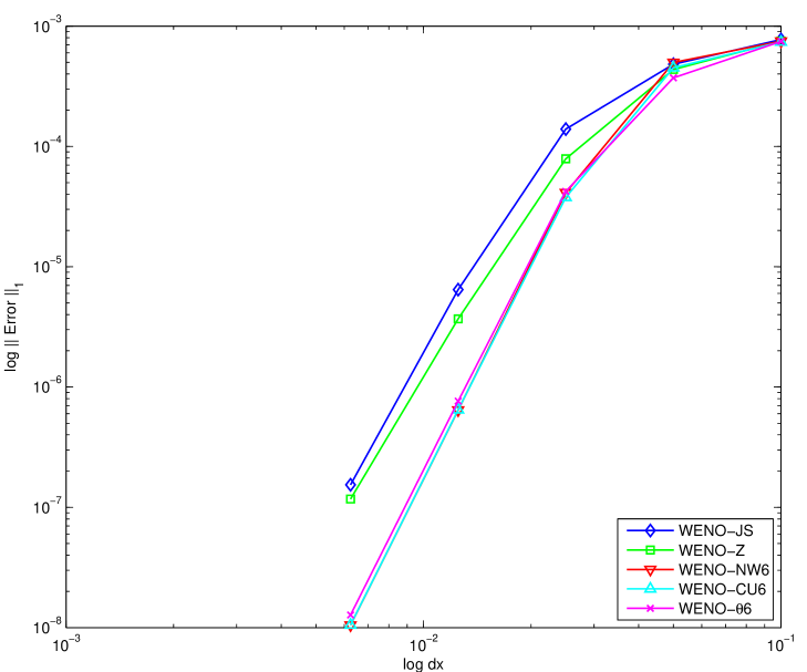
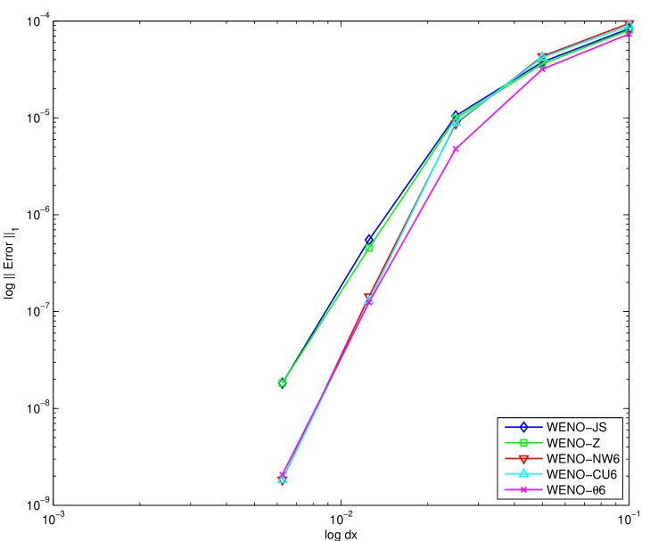
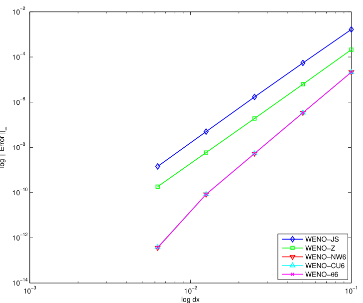
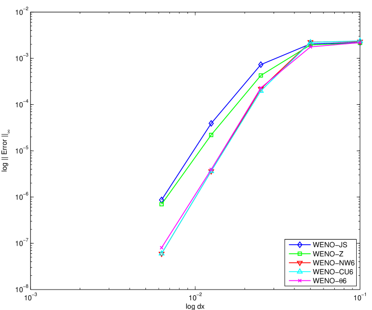
Figure 4. Convergence of Eq. (3.20) at time $t=1$. Left: Initial condition (3.21); Middle: Initial condition (3.22) with $k=2$. Right: Initial condition (3.22) with $k=3$. Top: in $L^{1}$ norm; Bottom: in $L^{\infty}$ norm.

3.3. Resolution Tests

We now test if our new scheme overcomes the loss of accuracy of WENO-CU6 and WENO-NW6. We revisit the initial condition given in example 1.1 which is as follows,

(3.23) $$u_{0}(x)=\max(\sin(\pi x),0),\quad x\in(-1,1).$$

The numerical solution obtained from our new scheme is added and shown in Fig. 5, together with those given in example 1.1. We also plot the pointwise errors in $L^{\infty}$ norm in the same figure. It is shown that WENO-$\theta 6$ approximates the critical region around $x=-0.1$ much better than WENO-CU6 and WENO-NW6. Indeed, the pointwise errors of the former around this region is comparable to those of WENO-JS and WENO-Z, where WENO-NW6 and WENO-CU6 show a loss of accuracy, which in turn causes problems for approximating solutions where symmetry is required. See below tests for numerical evidence.

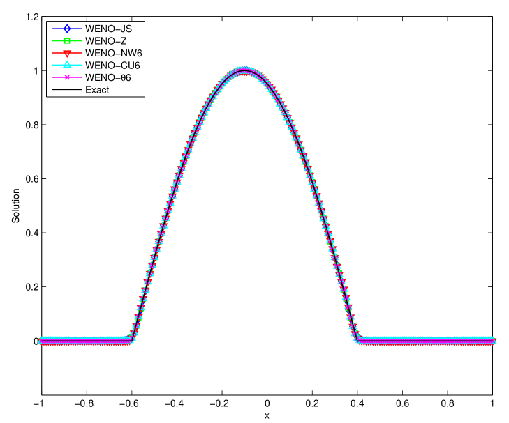
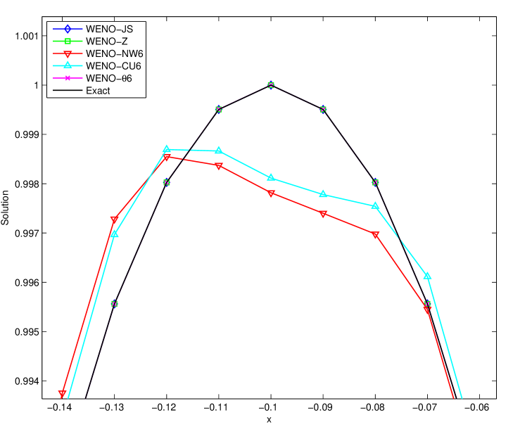
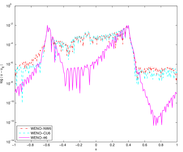
Figure 5. Left: Numerical solutions of Eq. (2.1) with initial condition (3.23) at time $t=2.4$. Grid $200$. Middle: Zoom near the critical point. Right: Pointwise errors in log scale.

The nonlinear weights $\omega_{k}$’s of these schemes are plotted in Fig. 6. We observe that around the critical point, the $\omega_{k}$’s of WENO-Z and WENO-$\theta 6$ are stable and converge to their optimal values $\gamma_{k}$’s. We note that for the latter scheme, the nonlinear weights keep fluctuating between the optimal weights of the 5th-order upwind and 6th-order central linear schemes. This clearly shows the effect of switching mechanism (3.19) in improving the accuracy of the scheme near the critical region. We also notify the non-convergence of $\omega_{k}$’s of the WENO-CU6 and WENO-NW6 schemes around the critical region. This shows the improvement of our new scheme over the other 6th-order ones.

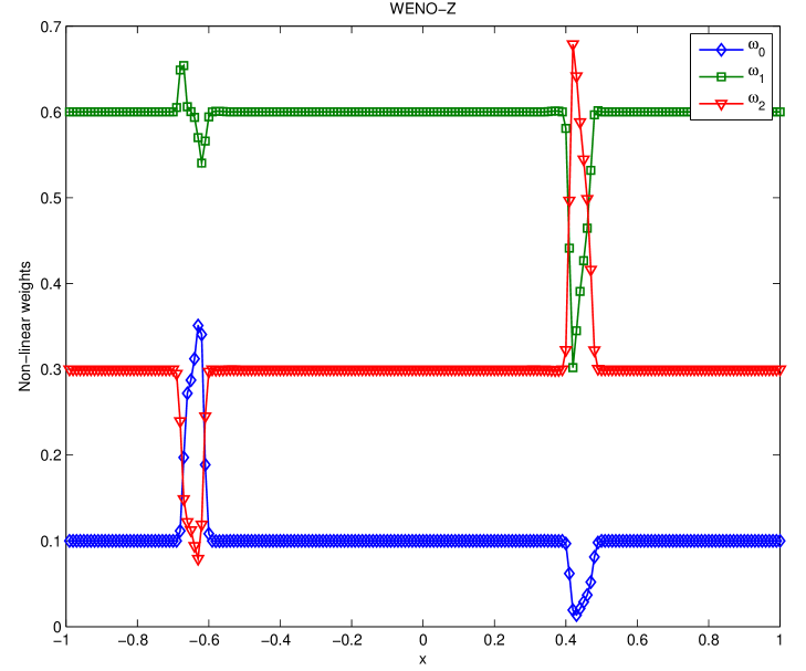
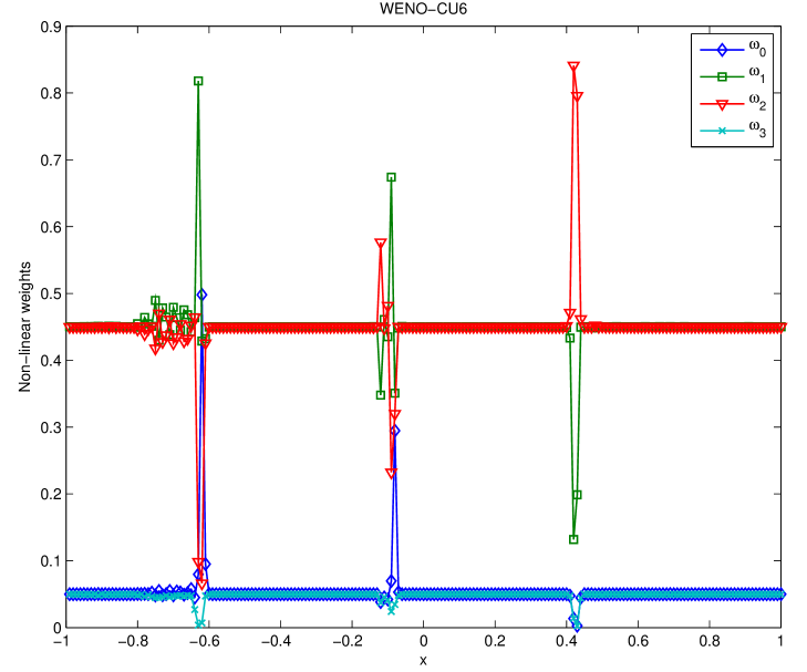
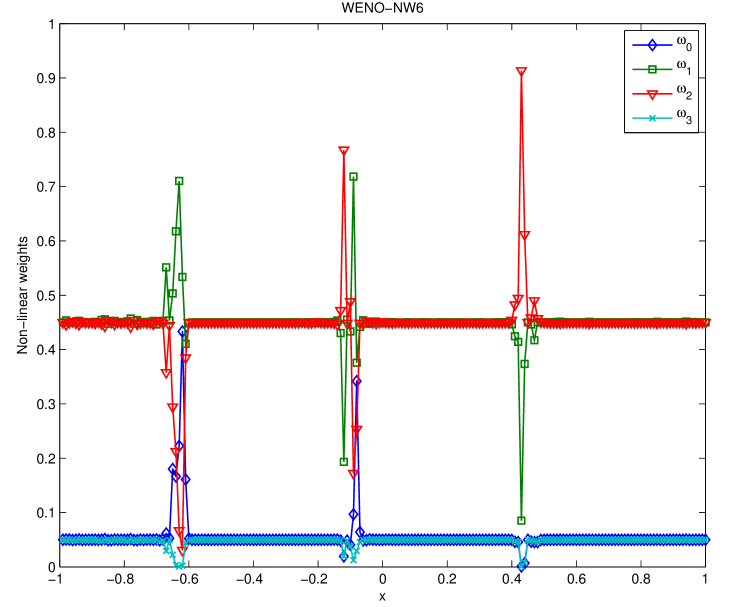
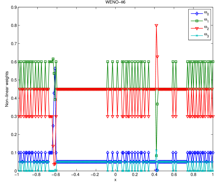
Figure 6. Distribution of the non-linear weights for the initial data (3.23). From top to bottom, left to right: WENO-Z, WENO-CU6, WENO-NW6, and WENO-$\theta$6.

4. Numerical Results

In this section, we perform a number of tests to compare the results of our new scheme with those obtained from the other WENO schemes, including the 5th-order upwind WENO-JS, WENO-Z, and the 6th-order central WENO-CU6, WENO-NW6.

4.1. Scalar Conservation Laws

4.1.1. TEST 1: Linear Case

We solve the one-dimensional linear advection equation (3.20) with the following initial condition $u_{0}(x)$ which contains a $C^{\infty}$ Gaussian, a square wave, a triangle, and a semi-ellipse (see [JS96]),

(4.1) $$u_{0}(x)=\begin{cases}&\frac{1}{6}[G(x,\beta,z-\delta)+4G(x,\beta,z)+G(x,\beta,z+\delta)],\quad-0.8\leq x\leq-0.6,\\ &1,\quad\quad\quad\quad\quad\quad\quad\quad\quad\quad\quad\quad\quad\quad\quad\quad\quad\quad\quad\quad\ \ -0.4\leq x\leq-0.2,\\ &1-|10(x-0.1)|,\quad\quad\quad\quad\quad\quad\quad\quad\quad\quad\quad\quad\quad\quad 0\leq x\leq 0.2,\\ &\frac{1}{6}[F(x,\alpha,a-\delta)+4F(x,\alpha,a)+F(x,\alpha,a+\delta)],\quad 0.4\leq x\leq 0.6,\\ &0,\quad\quad\quad\quad\quad\quad\quad\quad\quad\quad\quad\quad\quad\quad\quad\quad\quad\quad\quad\quad\ \ \text{otherwise},\end{cases}$$

where

(4.2) $$G(x,\beta,z)=\exp(-\beta(x-z)^{2}),$$

(4.3) $$F(x,\alpha,a)=\sqrt{\max(1-\alpha^{2}(x-a)^{2},0)};$$

the constants are $z=-0.7$, $\delta=0.005$, $\beta=\frac{\log 2}{36\delta^{2}}$, $a=0.5$, and $\alpha=10$.

We compute the solution up to time $t=6.3$ with $N=400$ and periodic boundary conditions. The results obtained from the WENO-CU6, WENO-NW6, and WENO-$\theta 6$ schemes are plotted in Fig. 7. We choose $\alpha_{R}=50$. Zooms around the shocks and top of the semi-ellipse are also shown in the same figure. It is observed that WENO-$\theta 6$ is comparable to WENO-NW6 in capturing the shocks, but the former is much better than the latter and WENO-CU6 in approximating top of the semi-ellipse.

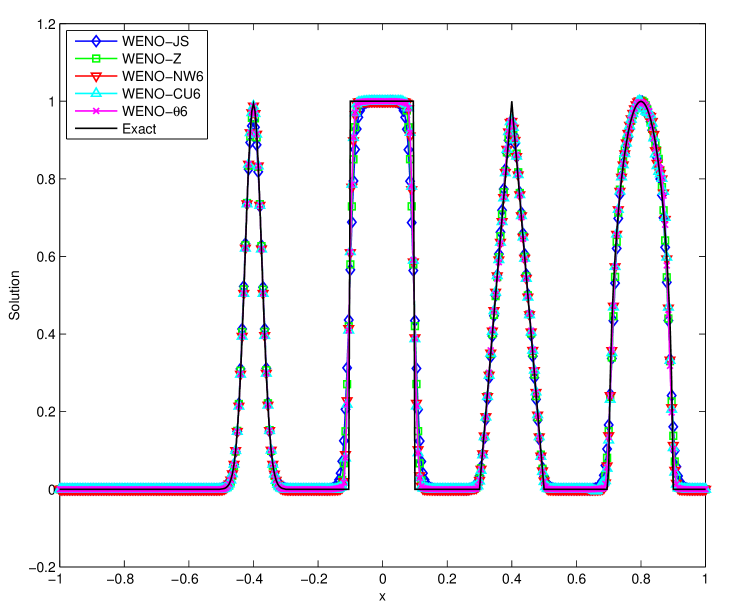
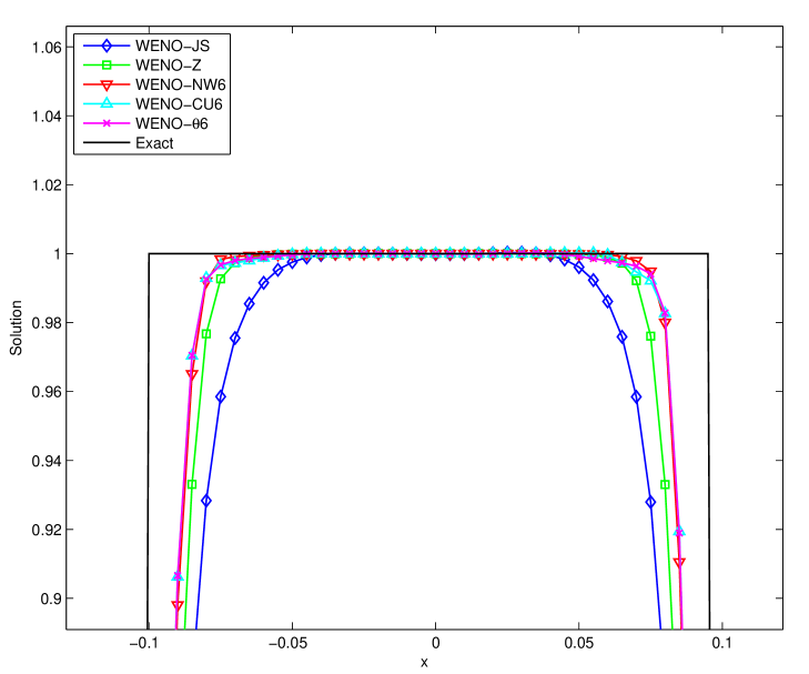
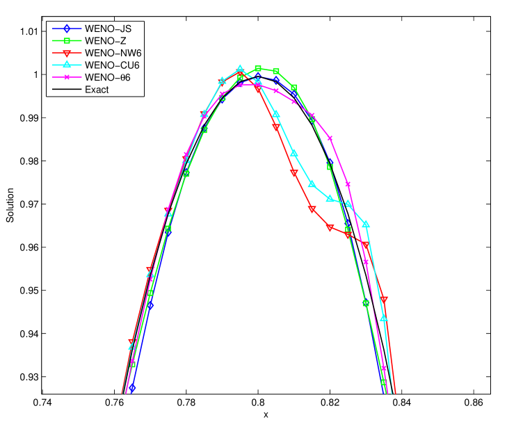
Figure 7. Left: Linear advection Eq. (3.20) with initial condition (4.1). Time $t=6.3$. Grid $400$. The others: zooms at critical regions.

4.1.2. TEST 2: Nonlinear Case

For this, we choose the Burgers equation

(4.4) $$\begin{cases}u_{t}+\left(\dfrac{u^{2}}{2}\right)_{x}=0,\quad x\in(-1,1),\\ u(x,0)=u_{0}(x),\end{cases}$$

subject to periodic boundary conditions.

In Fig. 8, we show the numerical results of the 6th-order WENO schemes for the initial condition

(4.5) $$u_{0}(x)=-\sin(\pi x);$$

at time $t=1.5$ and

(4.6) $$u_{0}(x)=\dfrac{1}{2}+\sin(\pi x)$$

at $t=0.55$. We choose a grid of $N=200$ grid intervals and $\alpha_{R}=50$. It is shown that the shocks are very well captured by all schemes.

Figure 8. Burgers’ Eq. (4.4). Grid $200$. Left: initial condition (4.5) at time $t=1.5$; Right: initial condition (4.6) at time $t=0.55$.

4.2. Euler Equations of Gas Dynamics

In this subsection, we consider the one-dimensional Euler equations of gas dynamics given in the following,

(4.7) $$\mathbf{u}_{t}+\mathbf{f}(\mathbf{u})_{x}=0,$$

where

(4.8) $$\mathbf{u}=(\rho,\rho u,E)^{T},\quad\mathbf{f}(\mathbf{u})=(\rho u,p+\rho u^{2},(E+p)u)^{T},$$

where $\rho$, $u$, $p$, $E$ are density, velocity, pressure, and total energy, respectively. The equation of state is as follows,

(4.9) $$p=(\gamma-1)\left(E-\dfrac{1}{2}\rho u^{2}\right),\quad\gamma=1.4,$$

where $\gamma$ is the ratio of specific heats. More details on the Euler equations can be found in, e.g., [LV92], [To97].

For all below numerical simulations, we apply the WENO schemes in characteristic fields of the flux $\mathbf{f}(\mathbf{u})$. That is, we first find an average of the Jacobian $A_{j+\frac{1}{2}}$ at the interface $x=x_{j+\frac{1}{2}}$. For this, we apply the Roe’s mean matrix (see [Ro81]). Then the eigenvalues $\lambda_{s}$’s, $L=[\mathbf{l}_{s}]_{s=1}^{m}$, $R=[\mathbf{r}_{s}]_{s=1}^{m}$ the complete sets of the left and right eigenvectors, respectively, of $A_{j+\frac{1}{2}}$ are determined. We next project the flux $\mathbf{f}(\mathbf{u})$ into the characteristic fields by left multiplying it with $L$. WENO schemes with a global Lax-Friedrichs flux splitting are applied to approximate the components of the flux. After that, the approximation in each characteristic field is projected back to the component space by a right multiplying with the matrix $R$.

4.2.1. TEST 3: Riemann Problems

We consider the shock-tube problems which are Eq. (4.7) with Riemann initial data. In particular, the Sod problem, the Lax problem, and the $123$ problem are given below.

$\bullet$ Sod’s problem:

(4.10) $$(\rho,u,p)=\begin{cases}&(0.125,\ \ 0,\ \ 0.1),\quad-5<x<0,\\ &(1,\ \ 0,\ \ 1),\quad 0<x<5;\end{cases}$$

and the final time $t=1.7$.

$\bullet$ Lax’s problem:

(4.11) $$(\rho,u,p)=\begin{cases}&(0.445,\ \ 0.698,\ \ 3.528),\quad-5<x<0,\\ &(0.5,\ \ 0,\ \ 0.571),\quad 0<x<5;\end{cases}$$

and the final time $t=1.3$.

$\bullet$ 123 problem:

(4.12) $$(\rho,u,p)=\begin{cases}&(1,\ \ -2,\ \ 0.4),\quad-5<x<0,\\ &(1,\ \ 2,\ \ 0.4),\quad 0<x<5;\end{cases}$$

and the final time $t=1$.

We apply a transmissive condition at both boundaries. The exact solution of these shock-tube problems can be found in, for example, [To97]. For Lax’s and the blast waves problems, we choose $\alpha_{R}=10$; and $\alpha_{R}=50$ for other problems.

Numerical results of the density obtained from all WENO schemes with a grid of $N=300$ are shown in Figs. 9 - 11, respectively. We observe that for Sod’s and Lax’s problems, there are overshoots at the contact discontinuities for WENO-CU6, whereas WENO-$\theta 6$ gives the sharpest capturing without generating oscillations. For the $123$ problem, WENO-CU6 shows the most wiggling behavior around the trivial contact discontinuity.

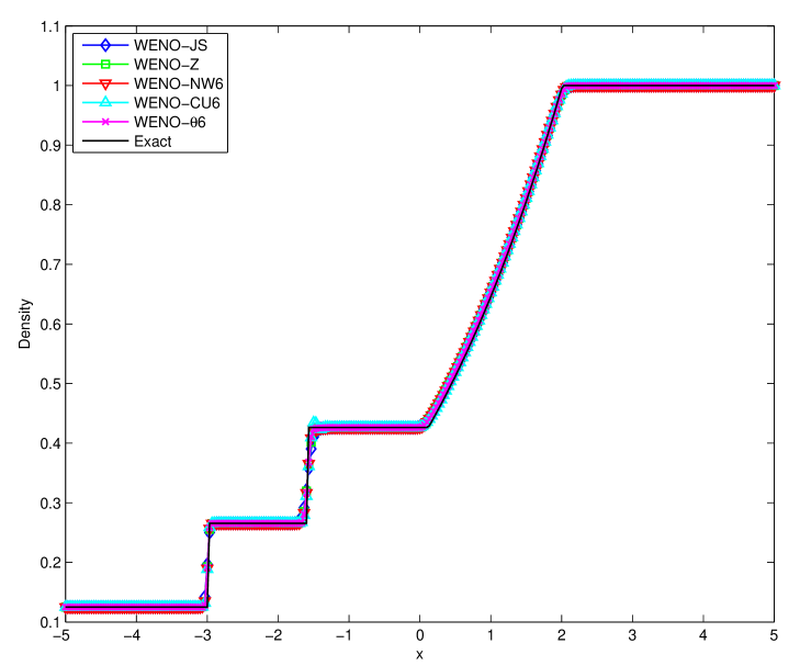
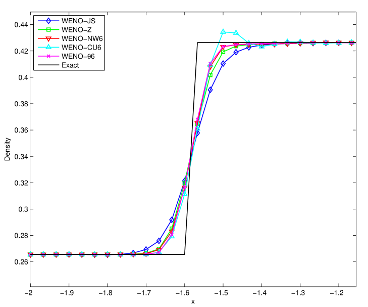
Figure 9. Left: Sod’s problem with initial data (4.10). Time $t=1.7$. Grid $300$. Right: zoom at the contact discontinuity.

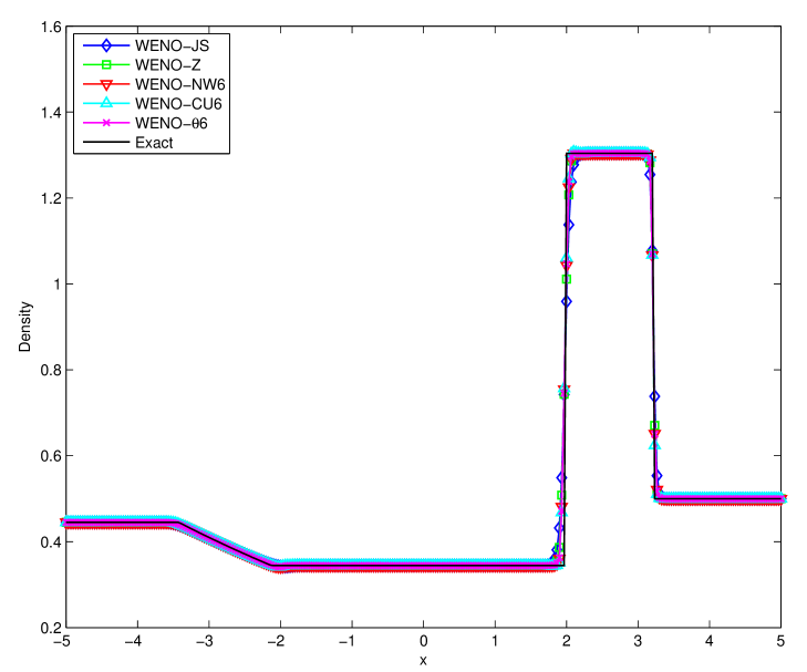
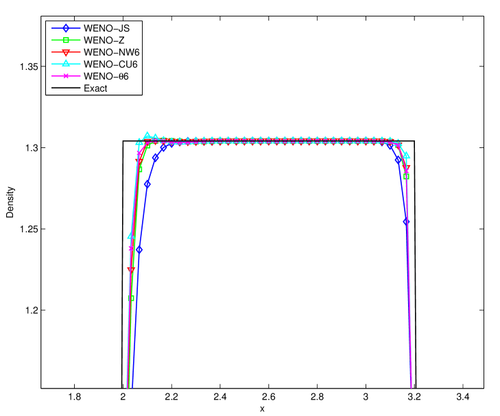
Figure 10. Left: Lax’s problem with initial data (4.11). Time $t=1.3$. Grid $300$. Right: zoom at the contact discontinuity.

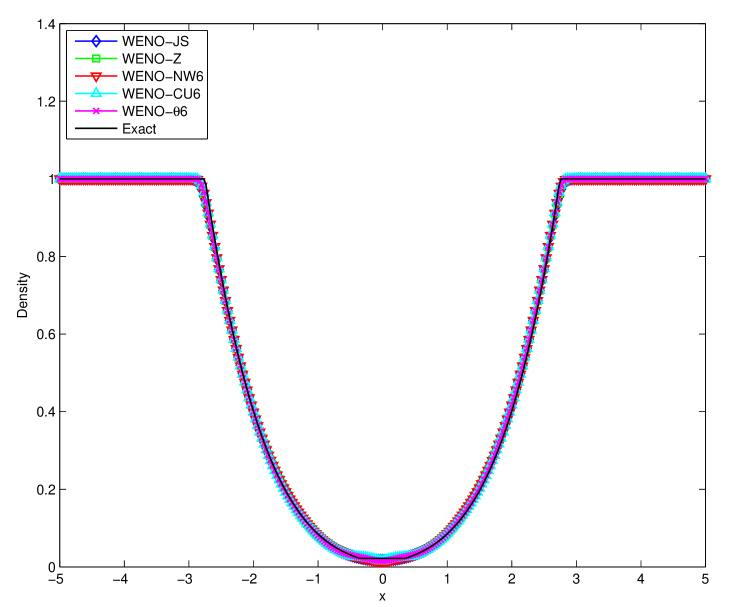
Figure 11. Left: The $123$ problem with initial data (4.12). Time $t=1.0$. Grid $300$. Right: zoom at the trivial contact discontinuity.

4.2.2. TEST 4: Shock Density Wave Interaction, Shu-Osher’s test

We consider the following initial data,

(4.13) $$(\rho,u,p)=\begin{cases}&(3.857143,\ \ 2.629369,\ \ 31/3),\quad-5<x<-4,\\ &(1+0.2\sin(5x),\ \ 0,\ \ 1),\quad-4<x<5,\end{cases}$$

with zero-gradient boundary conditions.

The problem simulates the interaction of a right-moving Mach 3 shock with a wavelike perturbed density whose magnitude is much smaller than the shock. As a result, a flow field of compressed and amplified wave trails is created right behind the shock. For more details, see [JS96]. In Fig. 12, we show the numerical results of the 6th-order WENO schemes at time $t=1.8$ with grids of $N=200$ and $N=400$ intervals. The “exact” solution is computed by WENO-JS with a fine grid $N=4000$. It is shown that all schemes give satisfactory approximations of the compressed wavelike structures behind the shock. A careful observation reveals that WENO-$\theta 6$ resolves the wave package as well as WENO-CU6, whereas WENO-NW6 is more dissipative for both grid levels.

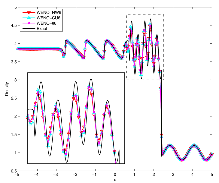
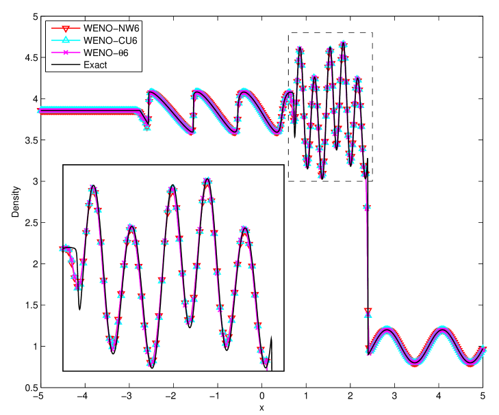
Figure 12. Shu-Osher’s problem with initial data (4.13). Density. Time $t=1.8$. Left: medium grid $200$; Right: fine grid $400$.

4.2.3. TEST 5: Two Interacting Blast Waves

In this test, we show that our new scheme WENO-$\theta 6$ passes the tough test of two interacting blast waves which the initial data are given as follows,

(4.14) $$(\rho,u,p)=\begin{cases}&(1,\ \ 0,\ \ 1000),\quad 0<x<0.1,\\ &(1,\ \ 0,\ \ 0.01),\quad 0.1<x<0.9,\\ &(1,\ \ 0,\ \ 100),\quad 0.9<x<1,\end{cases}$$

and a reflective condition is applied at both boundaries. This problem is used to test the robustness of shock-capturing methods since many interactions are observed in a small area. A detailed discussion of this problem can be found in [WC84].

Numerical results of 6th-order WENO schemes are computed up to time $t=0.038$ with a grid of $N=801$ and plotted in Fig. 13 for the density. The exact solution is approximated by WENO-JS with a much fine grid $N=4001$. It is shown that all schemes well capture the shocks as well as contact discontinuities. A zoom near $x=0.745$ indicates that WENO-$\theta 6$ gives better resolution than WENO-NW6 and WENO-CU6. We also emphasize that there exists a stair-casing phenomenon in the solutions of the latter methods in this region, which is similar to that at the top of the semi-ellipse in test $1$ (see Fig. 7), and the $123$ problem (see Fig. 11).

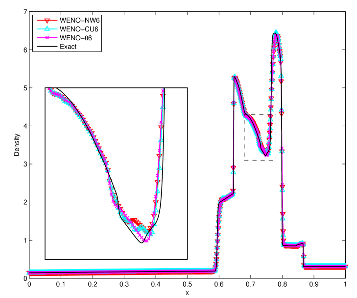
Figure 13. Two interacting blast waves with initial data (4.14). Density. Time $t=0.038$. Grid $801$.

4.3. Two-dimensional Euler’s Equations

In this subsection, we extend the problem to two-dimensional cases. We choose the 2D Euler equations which are as follows,

(4.15) $$\begin{cases}&\mathbf{u}_{t}+\mathbf{f}(\mathbf{u})_{x}+\mathbf{g}(\mathbf{u})_{y}=0,\\ &\mathbf{u}(x,y,0)=\mathbf{u}_{0}(x,y),\end{cases}$$

where $\mathbf{u}=(\rho,\rho u,\rho v,E)^{T}$, $\mathbf{f}(\mathbf{u})=(\rho u,p+\rho u^{2},\rho uv,u(E+p))^{T}$, $\mathbf{g}(\mathbf{u})=(\rho v,\rho uv,p+\rho v^{2},v(E+p))^{T}$. The relation of pressure and conservative quantities is through the equation of state

(4.16) $$p=(\gamma-1)\left(E-\dfrac{1}{2}(u^{2}+v^{2})\right).$$

Here, we choose the ratio of specific heats $\gamma=1.4$.

4.3.1. TEST 6: Rayleigh-Taylor Instability

In the following tests, we show numerical evidence that WENO-$\theta 6$ maintains symmetry in the solutions much better than the other 6th-order schemes, and outperforms 5th-order schemes in resolving small-scaled structures occurring in flow configurations. We first simulate the Rayleigh-Taylor instability. The instability occurs where there is a heavy fluid falling into a light fluid (see [GGLO88], [At], [FSTY14]). Following [At], we set up the problem as follows. The domain is $(x,y)=(-0.25,0.25)\times(-0.75,0.75)$. Initial density has a discontinuity at the interface, i.e., $\rho=2$ for $y\geq 0$ and $\rho=1$ for $y<0$. The pressure is set at hydrostatic equilibrium initially $p=2.5-\rho gy$ where $g=0.1$ is the gravitational acceleration. The $x$-component velocity $u=0$, while the $y$-component is perturbed with $v=\frac{0.01}{4}(1+\cos(4\pi x))(1+\cos(\frac{4}{3}\pi y))$ for a single mode perturbation. Boundary conditions are set periodic in $x$-direction, and reflective in $y$-direction. The ratio of specific heats $\gamma=1.4$. We add $-g\rho$ and $-g\rho v$ in the $y$-momentum and energy equations of (4.15) as source terms.

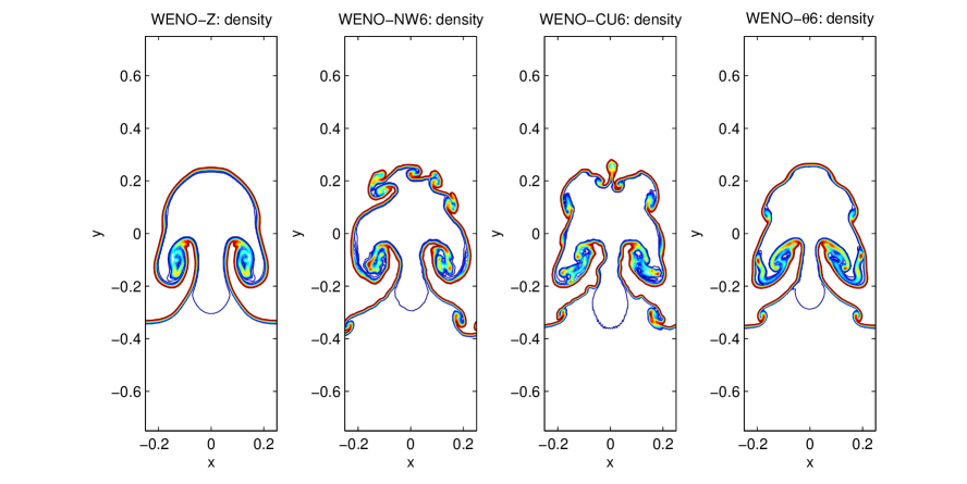
Figure 14. The Rayleigh-Taylor instability. Density at time $t=9.5$. Grid $120\times 360$. $CFL=0.5$. From left to right: WENO-Z, WENO-NW6, WENO-CU6, and WENO-$\theta 6$.

In Fig. 14, we plot the density with 20 equally spaced contours obtained from 5th- and 6th-order WENO schemes at time $t=9.5$ with a $120\times 360$ grid. It is shown that the 6th-order schemes have much better numerical resolution comparing with the 5th-order ones. We notice that WENO-$\theta 6$ preserves the symmetry of the solution; whereas WENO-NW6 and WENO-CU6 do not. We conjecture the lack of symmetry of WENO-NW6 is due to the loss of accuracy around critical regions which is shown in previous numerical tests. The test also shows that the discontinuous switching of $\tau^{\theta}$ in Eq. (3.19) does not affect the robustness of the new WENO-$\theta$ scheme, even for problem with highly unstable fluid flows as the Rayleigh-Taylor instability.

4.3.2. TEST 7: Implosion problem

The next numerical test is the implosion problem (see [At], [LW04]) with initial data as follows,

(4.17) $$(\rho,p)=\begin{cases}&(1,1)\quad\text{for }x+y>\frac{1}{2},\\ &(0.125,0.14)\quad\text{otherwise},\end{cases}$$

and zero velocity everywhere initially. We choose reflecting conditions for all boundaries.

Symmetry is important for this test. For such a scheme, due to the interactions of shock waves and reflecting boundaries, jets along the diagonal are created. Longer and narrower jets are produced for less dissipative schemes.

In Fig. 15, we show the results obtained from different schemes on computational domain $(0,1)\times(0,1)$ at final time $t=5$. We choose a grid of $400\times 400$. For WENO-$\theta$, we choose $\alpha_{R}=1$. It is shown that only WENO-Z and WENO-$\theta$ well preserve the symmetry of the problem; whereas the other 6th-order schemes do not. The jets created by WENO-NW6 and WENO-CU6 tend to diverge from the main diagonal $x=y$. We also note that the jets produced by WENO-$\theta$ is much longer and narrower than those of WENO-Z, which means that the former scheme is less dissipative than the latter one.

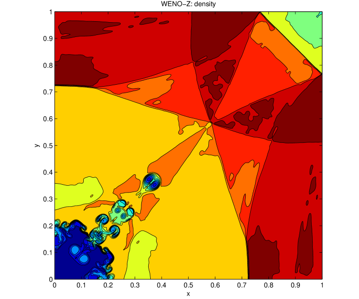
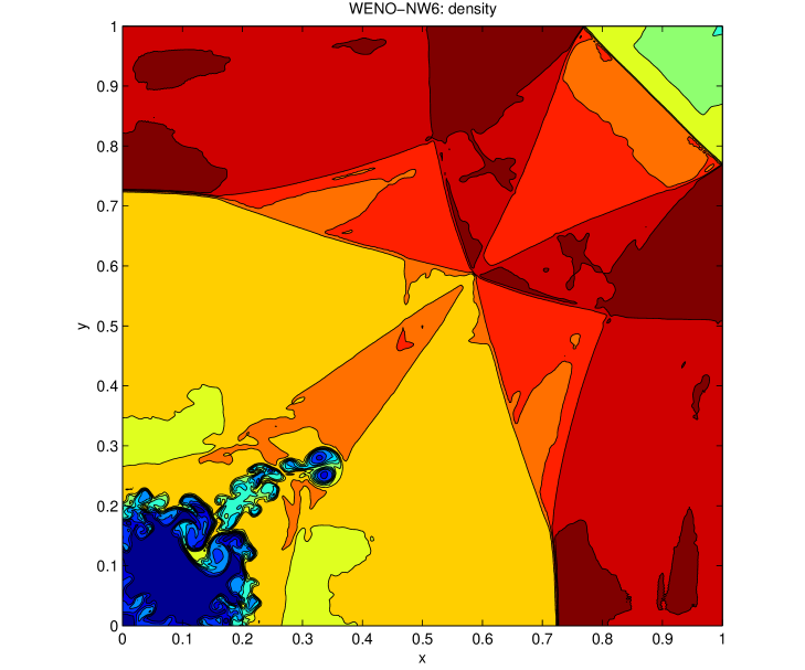
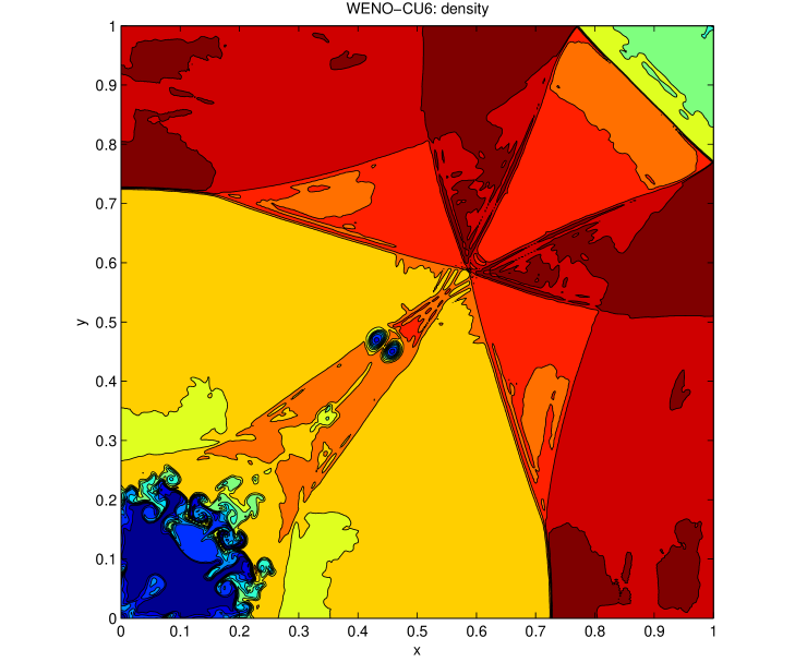
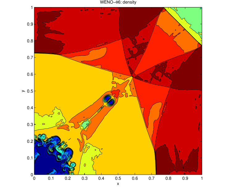
Figure 15. The implosion problem. Density with 20 contours uniformly distributing from $0$ to 1. Grid $400\times 400$. Final time $t=5$. Left to right, top to bottom: WENO-Z, WENO-NW6, WENO-CU6, WENO-$\theta$6.

4.3.3. TEST 8: 2D Riemann Initial Data

The 2D Riemann problem is set up by assigning different constant states of $(\rho_{k},u_{k},v_{k},p_{k})$, $k=1,2,3,4$, to four quadrants of the computational domain $\Omega=(0,1)\times(0,1)$. The constant states are chosen so that there is only a single elementary wave, namely, shock-, rarefaction-, and contact-wave, connecting two neighboring quadrants (see [SCG93]). For our test, we choose the following configuration for the initial data, respectively, for quadrants $1$, $2$, $3$, $4$,

(4.18) $$(\rho,u,v,p)=\begin{cases}&(0.5313,\ 0,\ 0,\ 0.4),\ \quad x>0.5,\ y>0.5,\\ &(1,\ 0.7276,\ 0,\ 1),\quad\quad x<0.5,\ y>0.5,\\ &(0.8,\ 0,\ 0,\ 1),\ \ \quad\quad\quad x<0.5,\ y<0.5,\\ &(1,\ 0,\ 0.7276,\ 1),\ \ \ \quad x>0.5,\ y<0.5,\end{cases}$$

which has shocks through quadrants $1$ - $2$ and $1$ - $4$, and contact discontinuities through quadrants $2$ - $3$ and $3$ - $4$. Transmissive boundary conditions are imposed on all boundaries for these two cases.

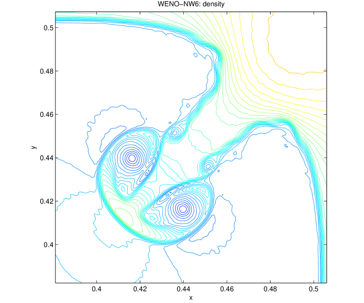
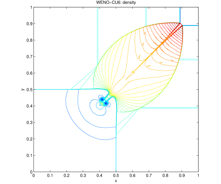
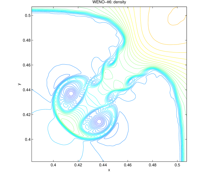
Figure 16. Left: The 2D Riemann problem with initial data (4.18). Density with $50$ contours. Time $t=0.25$. Grid $1000\times 1000$. Right: Zoom at the spirals. From top to bottom, respectively: WENO-NW6, WENO-CU6, WENO-$\theta$6.

The approximations of the density with initial data (4.18) at time $t=0.25$ are plotted in Fig. 16 with $50$ contours for WENO-NW6 and WENO-$\theta$6. Here, we use a fine grid with $1000\times 1000$ intervals for the capturing of the small vortices along the contacts. Zooms near the spirals region are also shown on the right column in the same figure. Again, we observe a better performance of the WENO-$\theta$6 over WENO-NW6 and WENO-CU6 schemes over these small-scaled structures without oscillations on the contours.

4.3.4. TEST 9: Double Mach Reflection of a Strong Shock

Finally, we investigate the double Mach reflection of a strong shock which is a typical benchmark test for shock-capturing methods. The problem simulates the reflection occurring when a simple planar shock interacts with a wedge making with the $x$-axis an angle $\alpha$. The strength of the moving shock is characterized by the Mach number $M_{s}$. For a double Mach reflection problem, $M_{s}=10$ and the wedge angle is chosen as $\alpha=30^{\circ}$. Detailed discussions on this type of problems can be found in [WC84] and the references therein. For numerical purpose, we choose the computational domain $\Omega=(0,4)\times(0,1)$. Initially the shock is located at $x_{0}=1/6$, inclined with the $x$-axis by the angle $90^{\circ}-\alpha$. Inflow and zero gradients conditions are imposed on the left and right boundaries, respectively. On the bottom one, a reflective condition is applied to the interval $[x_{0},4]$ representing the wedge, and the exact post-shock state is imposed over $[0,x_{0}]$. The top boundary is treated in a way that there are no interactions of the shock with this boundary. That is, the exact post- and pre-shock states are employed over the intervals $[0,x_{s}(t)]$ and $[x_{s}(t),4]$, respectively, on the top boundary. Here, $x_{s}(t)=x_{0}+\dfrac{1}{\tan 60^{\circ}}+\dfrac{M_{s}a_{pre}}{\cos 30^{\circ}}t$, where $a_{pre}$ is the sound speed of the pre-shock state, is the location of the shock in time. These states can be computed exactly when one of them is pre-described (see, e.g., [To97]). In particular, for our problem the initial conditions are given as follows,

(4.19) $$(\rho,u,v,p)=\begin{cases}&(8,\ 8.25\cos 30^{\circ},\ -8.25\sin 30^{\circ},\ 116.5),\quad x<x_{0}+\frac{y}{\tan 60^{\circ}},\\ &(1.4,\ 0,\ 0,\ 1),\quad\quad\quad\quad\quad\quad\quad\quad\quad\quad\quad\ x\geq x_{0}+\frac{y}{\tan 60^{\circ}}.\end{cases}$$

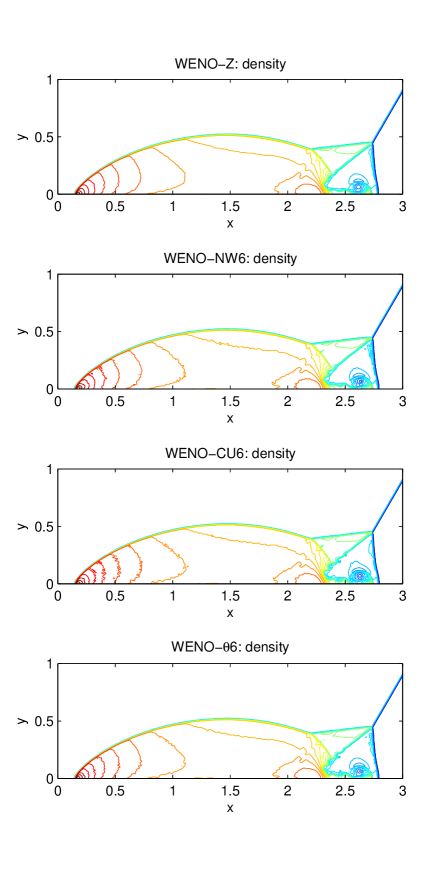
Figure 17. The double-Mach reflection problem with initial data (4.19). Density with $30$ contours. Time $t=0.2$. Grid $800\times 200$. From top to bottom, respectively: WENO-Z, WENO-NW6, WENO-CU6, and WENO-$\theta$6.

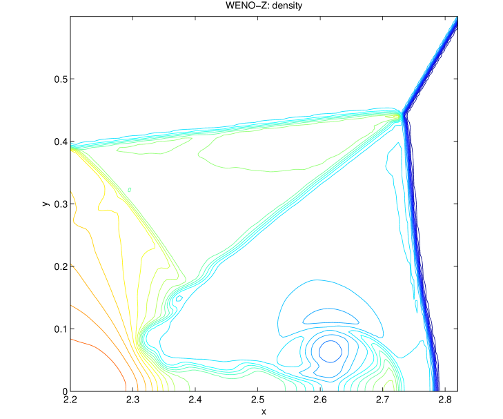
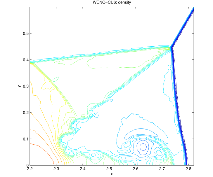
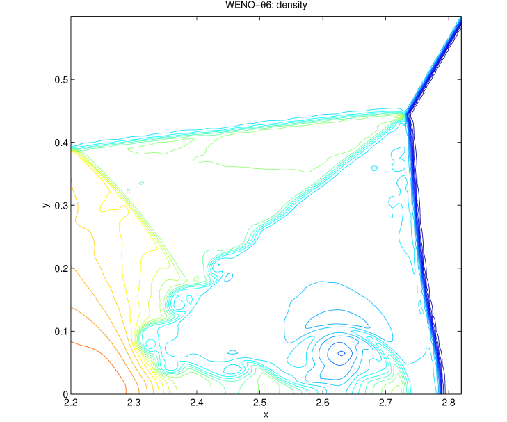
Figure 18. The double-Mach reflection problem with initial data (4.19). Zoom at the double Mach stems region. From top to bottom, respectively: WENO-Z, WENO-NW6, WENO-CU6, and WENO-$\theta$6.

Numerical results of the density obtained from the 5th-order WENO-Z, the 6th-order WENO-NW6, WENO-CU6, and WENO-$\theta$6 schemes at time $t=0.2$ are plotted in Fig. 17 with $30$ contours. For this case, we choose a fine grid of $800\times 200$ points for all schemes. We notice the rendering of small vortices at the end of the slip line and the wall jet, starting from WENO-Z and becoming clearer for the 6th-order schemes. The zoom-in on the Mach stems region shown in Fig. 18 reveals that the WENO-$\theta$6 scheme gives more satisfactory resolution than the WENO-NW6 and WENO-CU6 ones.

5. Conclusion

In this work, we have presented a new WENO-$\theta$ scheme which adaptively switches between a 5th-order upwind and 6th-order central scheme, depending on the smoothness of not only the sub-stencils but also the large one. Unlike the other 6th-order WENO methods in which this switch depends solely on the smoothness of the most downwind sub-stencil, it is that of the large stencil which decides this mechanism in our new scheme. Main features of our new scheme are that the new scheme combines good properties of both 5th-order upwind and 6th-order central schemes. That is, the new scheme is more dispersive than the 5th-order ones in terms of better resolution of small-scaled structures and capturing discontinuities. Moreover, the scheme overcomes the loss of accuracy around some critical regions and has the ability to maintain symmetry in the solutions which are drawbacks of other comparing 6th-order WENO schemes.

We have also developed the new smoothness indicators of the sub-stencils $\tilde{\beta}_{k}$’s which are symmetric in terms of Taylor expansions around the point $x_{j}$ and a new $\tau^{\theta}$ for the large stencil. The latter is chosen as the smoother one among two candidates which are computed based on the possible highest-order variations of the reconstruction polynomials in $L^{2}$ sense. From then, value of the parameter $\theta$ is determined to decide if the scheme is 5th-order upwind or 6th-order central.

A number of numerical tests for both scalar cases, linear and nonlinear, and system case with the Euler equations of gas dynamics are carried out to check the accuracy, resolution, and robustness of our new scheme. It is shown that our new method is more accurate than WENO-JS, WENO-Z, and WENO-CU6; more robust than WENO-CU6 and WENO-NW6; and outperforms comparing schemes in capturing small-scaled structures, and around critical regions.

Numerical simulations of higher dimensional problems will be investigated in a subsequent work. Since the new smoothness indicators $\tilde{\beta}_{3}$ and $\tau^{\theta}$ are constructed in a systematic manner, we expect a development of the scheme to a higher order of accuracy. This will be considered in our future work.

References

- [At] Athena3D in Fortran , http://www.astro.virginia.edu/VITA/athena.php.
- [BCCD08] R. Borges, M. Carmona, B. Costa, and W. S. Don, An improved weighted essentially non-oscillatory scheme for hyperbolic conservation laws, J. Comput. Phys. 227 (2008), 3191-3211.
- [BS00] D. S. Balsara, and C.-W. Shu, Monotonicity preserving weighted essentially non-oscillatory schemes with increasingly high order of accuracy, J. Comput. Phys. 160, 405-452 (2000).
- [CCD11] M. Castro, B. Costa, and W. S. Don, High order weighted essentially non-oscillatory WENO-Z schemes for hyperbolic conservation laws, J. Comput. Phys. 230 (2011), 1766-1792.
- [CD07] B. Costa, and W. S. Don, High order hydrid central - WENO finite difference scheme for conservation laws, IJCAM, 204 (2007), 209-218.
- [CFY13] M. H. Carpenter, T. C. Fisher, and N. K. Yamaleev, Boundary closures for sixth-order energy-stable weighted essentially non-oscillatory finite-difference schemes, Advances in Applied Mathematics, Modeling, and Computational Science, Fields Institute Communications Vol. 66, 2013, 117-160.
- [EP04] B. Epstein, and S. Peigin, Application of WENO (weighted essentially non-oscillatory) approach to Navier-Stokes computations, Int. J. Comput. Fluid D. 2004, Vol. 18 (3), 289-293.
- [Fa14] P. Fan, High order weighted essentially nonoscillatory WENO- schemes for hyperbolic conservation laws, J. Comput. Phys. 269 (2014), 355-285.
- [FHW12] H. Feng, F. Hu, and R. Wang, A new mapped weighted essentially non-oscillatory scheme, J. Sci. Comput. (2012), 51:449-473.
- [FSTY14] P. Fan, Y. Shen, B. Tian, and C. Yang, A new smoothness indicator for improving the weighted essentially non-oscillatory scheme, J. Comput. Phys., 269 (2014), 329-354.
- [GGLO88] J. Glimm, J. Grove, X. Li, W. Oh, and D. C. Tan, The dynamics of bubble growth for Rayleigh-Taylor unstable interfaces, Physics of Fluids 31 (1988), 447-465.
- [GS98] S. Gottlieb, and C.-W. Shu, Total variation dimishing Runge-Kutta schemes, Mathematics of Computation, Vol. 67, No. 221, (1998) 73-85.
- [Ha83] A. Harten, High resolution schemes for hyperbolic conservation laws, J. Comput. Phys. 49, 357-393 (1983).
- [Ha84] A. Harten, On a class of high resolution total-variation-stable finite-difference schemes, SIAM J. Numer. Anal., Vol. 21, No. 1, 1984.
- [HA11] X. Y. Hu, and N. A. Adams, Scale separation for implicit large eddy simulation, J. Comput. Phys., 230 (2011), 7240-7249.
- [HAP05] A. K. Henrick, T. D. Aslam, and J. M. Powers, Mapped weighted essentially non-oscillatory schemes: Achieving optimal order near critical points, J. Comput. Phys. 207 (2005), 542-567.
- [HEOC97] A. Harten, B. Engquist, S. Osher, and S. R. Chakravarthy, Uniformly high order accurate non-oscillatory schemes, III, J. Comput. Phys. 131, 3-47 (1997).
- [HKLY13] Y. Ha, C. H. Kim, Y. J Lee, and J. Yoon, An improved weighted essentially non-oscillatory scheme with a new smoothness indicator, J. Comput. Phys., 232 (2013), 68-86.
- [HP04] D. J. Hill, and D. I. Pullin, Hydrid tuned center-difference WENO method for large-eddy simulations in the presence of strong shocks, J. Comput. Phys. 194 (2004), 435-450.
- [HO87] A. Harten, and S. Osher, Uniformly high-order accurate nonoscillatory schemes, I, SIAM J. Numer. Anal., Vol. 24, No. 2, 1987, 279-309.
- [HOEC86] A. Harten, S. Osher, B. Engquist, and S. R. Chakravarthy, Some results on uniformly high-order accurate essentially nonoscillatory schemes, Applied Numerical Mathematics 2 (1986), 347-377.
- [HWA10] X. Y. Hu, Q. Wang, and N. A. Adams, An adaptive central-upwind weighted essentially non-oscillatory scheme, J. Comput. Phys., 229 (2010), 8952-8965.
- [JS96] G.-S. Jiang, and C.-W. Shu, Efficient implementation of Weighted ENO schemes, J. Comput. Phys. 126, 202-228 (1996).
- [LOC94] X.-D. Liu, S. Osher, and T. Chan, Weighted essentially non-oscillatory schemes, J. Comput. Phys. 115, 200-212 (1994).
- [LQ10] G. Li, and J. Qiu, Hydrid weighted essentially non-oscillatory schemes with different indicators, J. Comput. Phys., 229 (2010), 8105-8129.
- [LSZ09] Y.-Y. Liu, C.-W. Shu, and M.-P. Zhang, On the positivity of linear weights in WENO approximations, Acta Mathematicae Applicatae Sinica, English series, Vol. 25, No. 3 (2009), 503-538.
- [LV92] R. J. LeVeque, Numerical methods for conservation laws, 2nd ed., Lectures in Mathematics, ETH Zürich.
- [LW04] R. Liska, and B. Wendroff, Comparision of several difference schemes on 1D and 2D test problems for the Euler equations, SIAM J. Sci. Comput., 25 (3), 995-1017, 2003.
- [MTW06] M. P. Martín, E. M. Taylor, M. Wu, and V.G. Weirs, A bandwidth-optimized WENO scheme for the effective direct numerical simulation of compressible turbulence, J. Comput. Phys. 220 (2006), 270-289.
- [OC84] S. Osher, and S. Chakravarthy, High resolution schemes and the entropy condition, SIAM J. Numer. Anal., Vol. 21, No. 5, 1984.
- [Ro81] P. L. Roe, Approximate Riemann solvers, parameter vectors, and difference schemes, J. Comput. Phys. 43, 357-372 (1981).
- [Sh03] C.-W. Shu, High-order finite difference and finite volume WENO schemes and discontinuous Galerkin methods for CFD, Int. J. Comput. Fluid D., 2003, Vol. 17 (2), 107-118.
- [Sh09] C.-W. Shu, High order weighted essentially nonoscillatory schemes for convection dominated problems, SIAM Review, Vol. 51, No. 1, 82-126.
- [SCG93] C. W. Schulz-Rinne, J. P. Collins, and H. M. Glaz, Numerical solution of the Riemann problem for two-dimensional gas dynamics, SIAM J. Sci. Comput., Vol. 14, No. 6, pp. 1394-1414, 1993.
- [SHS02] J. Shi, C. Hu, and C.-W. Shu, A technique of treating negative weights in WENO schemes, J. Comput. Phys. 175, 108-127 (2002).
- [SZ08] Y. Shen, and G. Zha, A robust seventh-order WENO scheme and its applications, AIAA paper 2008-0757.
- [To97] E. F. Toro, Riemann solvers and numerical methods for fluid dynamics: A practical introduction, Springer-Verlag Berlin Heidelberg 1997.
- [TWM07] E. M. Taylor, M. Wu, and M. P. Martín, Optimization of nonlinear error for weighted essentially non-oscillatory methods in direct numerical simulations of compressible turbulence, J. Comput. Phys., 223 (2007), 384-397.
- [WC84] P. Woodward, and P. Colella, The numerical simulation of two-dimensional fluid flow with strong shocks, J. Comput. Phys. 54, 115-173 (1984).
- [YC09] N. K. Yamaleev, and M. H. Carpenter, A systematic methodology for constructing high-order energy stable WENO schemes, J. Comput. Phys. 228 (2009), 4248-4272.