Point Localization and Density Estimation from Ordinal kNN graphs using Synchronization

Abstract

We consider the problem of embedding unweighted, directed k-nearest neighbor graphs in low-dimensional Euclidean space. The k-nearest neighbors of each vertex provide ordinal information on the distances between points, but not the distances themselves. Relying only on such ordinal information, along with the low-dimensionality, we recover the coordinates of the points up to arbitrary similarity transformations (rigid transformations and scaling). Furthermore, we also illustrate the possibility of robustly recovering the underlying density via the Total Variation Maximum Penalized Likelihood Estimation (TV-MPLE) method. We make existing approaches scalable by using an instance of a local-to-global algorithm based on group synchronization, recently proposed in the literature in the context of sensor network localization, and structural biology, which we augment with a scale synchronization step. We show our approach compares favorably to the recently proposed Local Ordinal Embedding (LOE) algorithm even in the case of smaller sized problems, and also demonstrate its scalability on large graphs. The above divide-and-conquer paradigm can be of independent interest to the machine learning community when tackling geometric embeddings problems.

Index Terms—  k-nearest-neighbor graphs, ordinal constraints, graph embeddings, eigenvector synchronization

1 Introduction

Embedding unweighted $k$-nearest neighbor (kNN) graphs is a special case of ordinal or non-metric embedding, where one seeks a spatial embedding of $n$ points $\left\{\vec{x}_{i}\right\}_{i=1}^{n}$ in $\mathbb{R}^{d}$ such that

$$\forall(i_{1},j_{1},i_{2},j_{2})\in\mathcal{C},\hskip 7.22743pt\|\vec{x}_{i_{1}}-\vec{x}_{j_{1}}\|_{2}<\|\vec{x}_{i_{2}}-\vec{x}_{j_{2}}\|_{2},$$ (1)

where $\mathcal{C}$ denotes the set of ordinal constraints. Ordinal constraints are sometimes also specified as triplets [1]. In the case of unweighted kNN graph embedding, $\mathcal{C}=\mathcal{C}(G)=\left\{(a,b,a,c)\big{|}ab\in E(G),ac\not\in E(G)\right\},$ where $E(G)$ is the set of directed edges in the kNN graph $G$.

Graph-based methods are of utmost importance in several modern machine learning methods with applications such as clustering, dimensionality reduction, and ranking. Many such methods rely on weighted graphs, with weights often based on similarity functions, i.e., $w_{ij}=S(x_{i},x_{j})$. From a practical standpoint, storing unweighted kNN graphs instead would allow for a very sparse representation of the data. If one could recover the source data $\{x_{i}\}_{i=1}^{n}$ from unweighted kNN graphs, such a computationally efficient sparser representation would incur no information loss. Because of the extreme sparsity of the representation, this is generally a hard problem. Just recently, a method for recovering data distributions from unweighted kNN graphs was introduced in [2]. Another motivation for this problem comes from an instance of the popular sensor network localization problem, where each sensor is able to transmit only limited connectivity information to a central location (ID names of its k nearest neighbors), but transmits neither the distance measurements nor a complete list of all its neighbors within a given fixed radius.

The original work on this problem dates back to Shepard [3] and Kruskal [4, 5], and lately has been studied intensively in the machine learning literature [1, 6, 7, 8, 9, 10, 11, 12, 13, 14, 15, 16, 17]. In this work, we compare against and extend the recent Local Ordinal Embedding method [18], which enjoys several favorable comparisons with other modern methods. Another motivation for this problem comes from an instance of the popular sensor network localization problem, where each sensor is able to transmit only limited connectivity information to a central location, in the form of ID names of its k nearest neighbor sensors, but transmits neither the estimated distance measurements nor a complete list of all its neighbors within a given fixed radius. Note that either of these last two scenarios renders the localization problem (of estimating the sensor coordinates) easier to solve. Similar to the sensor network application, one could potentially apply this framework to cooperative control and sensing involving swarms of robot micro-vehicles with limited payloads communicating via radio with limited bandwidth [19, 20]. Our key ingredient is a modified version of the As-Synchronized-As-Possible (ASAP) algorithm introduced in [21], which makes existing embedding methods scalable via a divide-and-conquer, non-iterative local to global approach, reduces computational complexity, allows for massive parallelization of large problems, and increases robustness to noise. The ASAP algorithm introduced in [21], on which we rely in the present paper, renders our approach to reconstruct kNN graphs scalable to graphs with thousands or even tens of thousands of nodes, and is an example of a local-to-global approach that integrates local ordinal information into a global embedding calculation.

We detail in Section 3.1 the exact approach used to decompose the initial kNN graph into many overlapping subgraphs, that we shall refer to as patches from now on. Each resulting patch is then separately embedded in a coordinate system of its own using an ordinal embedding algorithm, such as the recent Local Ordinal Embedding (LOE) algorithm [18]. In the hypothetical scenario when LOE recovers the actual ground truth coordinates of each patch, such local coordinates agree with the global coordinates up to scaling and some unknown rigid motion (such as rotation, reflection and translation), in other words, up to a similarity transformation. However, in most practical instances, it is unreasonable to expect that the LOE algorithm will recover the exact coordinates only from ordinal data. On a related note, we point out the recent work of Kleindessner and von Luxburg [22], who settled a long-known conjecture claiming that, given knowledge of all ordinal constraints of the form $||x_{i}-x_{j}||<||x_{k}-x_{l}||$ between an unknown set of points $x_{1},\ldots,x_{n}\in\mathbb{R^{d}}$ (for finite $n$), it is possible to approximately recover the ground truth coordinates of the points up to similarity transformations. Furthermore, the same authors show that the above statement holds even when we only have local information such as the distance comparisons between points in small neighborhoods of the graphs, thus giving hope for a local-to-global approach, in the spirit of the one we propose in the present paper.

Our contributions are: 1. We present a local-to-global approach for the problem of embedding clouds of points from ordinal information, which is scalable to very large graphs, and can be computed efficiently and robustly in a distributed manner. Specifically, we extend the ASAP framework to the setting of ordinal embeddings, by augmenting it with a scale synchronization step. We believe that local-to-global strategies could benefit many problems in the machine learning community. The scale of data involved in many interesting problems poses a challenge to direct, holistic approaches. 2. We extend the ordinal embedding pipeline to perform density estimation via Total Varation Maximum Penalized Likelihood Estimation. This demonstrates the similarity between the point localization and density estimation problems. Sufficiently simple point distributions can be well estimated by applying a short postprocessing step to an approximate embedding. 3. We present preliminary results for a very simple, straightforward ordinal embedding method.

The rest of the paper is organized as follows. Section 2 is a summary of existing methods for related embedding problems. Section 3 details the pipeline of the ASAP framework, including the scale synchronization step in Section 3.2. In Section 4 we remark on the connection to the density estimation problem, and describe the post-processing step performed via Total-Variation Maximum Penalized Likelihood Estimation. Section 5 shows the results of several experiments recovering point embeddings from a variety of data sets, and compares to the existing LOE algorithm, as well as presenting results for the density estimation problem. In Section 6 we discuss an entirely different approach to ordinal embedding, and present some preliminary results which suggest more modifications are needed. We conclude our primary discussion in Section 7 and summarize in Appendix 7.1 some related basic notions from the rigidity theory literature.

2 Related Work

2.1 Multidimensional Scaling

Broadly speaking, multidimensional scaling (MDS) refers to a number of related problems and methods. In Classical Multidimensional Scaling (CMDS) [23], one is given all Euclidean Squared-Distance measurements $\Delta_{ij}=\|\vec{x}_{i}-\vec{x}_{j}\|_{2}^{2}$ on a set of points $X=\{\vec{x}_{i}\}_{i=1}^{n}$ and wishes to approximate the points, assuming that they approximately lie in a low-dimensional space $d\ll n$. Note that the solution for the coordinates is unique only up to rigid transformations, and that solutions do not exist for all possible inputs $\Delta$.

One can generalize CMDS to incorporate additional nonnegative weights $W_{ij}$ on each distance, useful when some distances are missing, or most distances are noisy, but some are known. The optimization involves minimizing an energy known in the literature as stress [24]. One approach to minimize stress is to iteratively minimize a majorizing function of two variables. A further generalization of MDS is non-metric MDS, or Ordinal Embedding, in which the input $D$ is assumed to be an increasing function applied to distance measurements [3]. This may be the case if $D$ represents dissimilarity between points, as opposed to measured distances. The problem can again be expressed with stress functionals and is usually solved with isotonic regresion [5].

2.2 Semidefinite Programming methods

Semidefinite Programming methods (SDP) have been applied frequently to MDS and related problems. Classical MDS can be stated as an SDP, with a closed form solution. Any formulation of the problem that optimizes over the Gram matrix requires the semidefinite constraint $K\in\mathbb{S}^{n}_{+}.$ Indeed, for metric MDS, if one penalizes the squared error on the squared distance measurements, the problem can be written as

$$\min_{X\in\mathbb{R}^{d\times n}}{\sum_{ij}W_{ij}(\Delta_{ij}-\Delta_{ij}(X))^{2}}$$

$$= \min_{K\in\mathbb{S}^{n}_{+},X\in\mathbb{R}^{d\times n}}{\sum_{ij}W_{ij}(\Delta_{ij}-(K_{ii}-2K_{ij}+K_{jj}))^{2}}$$

$$\mbox{ s.t. }K=X^{T}X.$$

Constraints of the form $K=X^{T}X$ are usually not allowed however, and are typically relaxed to [25, 26]

$$\left[\begin{matrix}I&X\\ X^{T}&K\end{matrix}\right]\succeq 0.$$

via Schur’s Lemma. Furthermore, one encourages $K$ to be approximately low-rank by introducing a nuclear norm or trace penalty $\|K\|_{*}=\|\sigma(K)\|_{1}=tr(K),$ as a convex relaxation of a rank constraint. Intuitively, since the $\ell_{1}$ norm promotes sparsity, the nuclear norm should promote few nonzero singular values. Elsewhere [27], it is argued that one should maximize $tr(K)$, in the spirit of the popular Maximum Variance Unfolding approach [27]. Neither minimizing nor maximizing the trace actually imposes an exact rank constraint, which is non-convex and NP-hard. One approach that could achieve exact rank constraints would be to use the Majorized Penalty Approach of Gao and Sun [28] with an alternating minimization method.

A group of methods have studied the graph realization problem, where one is asked to recover the configuration of a cloud of points given a sparse and noisy set of pairwise distances between the points [29, 30, 31, 32, 33]. One of the proposed approaches involves minimizing the following energy

$$\min_{p_{1},...,p_{n}\in\mathbb{R}^{2}}\sum_{(i,j)\in E}\left(\|p_{i}-p_{j}\|^{2}-d_{ij}^{2}\right)^{2}.$$ (2)

which unfortunately is nonconvex, but admits a convex relaxation into a SDP program. We refer the reader to Section 2 of [21] for several variations of this approach, some of which have been shown to be more robust to noise in the measured distances.

2.3 Local Ordinal Embedding

Terada and von Luxburg [18] have recently proposed an algorithm for ordinal embedding and kNN embedding specifically, called Local Ordinal Embedding (LOE), which minimizes a soft objective function that penalizes violated ordinal constraints.

$$\min_{X\in\mathbb{R}^{d\times n}}{\sum_{i<j,k<l,(i,j,k,l)\in\mathcal{C}}\max\left[0,D_{ij}(X)+\delta-D_{kl}(X)\right]^{2}}.$$ (3)

The energy takes into account not only the number of constraints violated, but the distance by which the constraints are violated, penalizing large violations more heavily.

An advantage of this energy in contrast to ones that normalize by the variance of $X$ (to guarantee nondegeneracy) is its relatively simple dependence on $X$, making the above energy easier to minimize. Instead, the scale parameter $\delta$ guarantees nondegeneracy, and fixes the scale of the embedding (which is indeterminable from ordinal data alone).

The authors introduce algorithms to minimizing the above energy, based on majorization minimization and the Broyden-Fletcher-Goldfarb-Shanno (BFGS) approximation of Newton’s method, and prove that ordinal embedding is possible when only local information is given (e.g. a $k$ neareast neighbor graph). The algorithm recovers not only the ordinal constraints, but the density structure of the data as well. The algorithm applies to ordinal constraints associated with $k$NN graphs as well more general sets of ordinal constraints. We will use this crucial property when solving subproblems in the method presented here, as the corresponding subgraphs are generally not $k$NN graphs.

3 ASAP & Scale Synchronization for Ordinal Embeddings

In this section we detail the steps of the ASAP algorithm, central to the divide-and-conquer algorithm we propose for the ordinal embedding problem. Note that the difference between the original ASAP algorithm introduced in [21] and our approach lies in the decomposition method from Section 3.1 and the scale synchronization step from Section 3.2. The ASAP approach starts by decomposing the given graph $G$ into overlapping subgraphs (referred to as patches), which are then embedded via the method of choice (in our case LOE). To every local patch embedding, there corresponds a scaling and an element of the Euclidean group Euc(d) of $d$-dimensional rigid transformations, and our goal is to estimate the scalings and group elements that will properly align all the patches in a globally consistent framework. The local optimal alignments between pairs of overlapping patches yield noisy measurements for the ratios of the above unknown group elements. Finding group elements from noisy measurements of their ratios is also known as the group synchronization problem. for which Singer [34] introduced spectral and semidefinite programming (SDP) relaxations over the group SO(2) of planar rotations, which is a building block for the ASAP algorithm [21].

Table 1 gives an overview of the steps of our approach. The inputs are an ordinal graph (we consider kNN graphs) $G=(V,E)$, where edge $ij\in E$ and non-edge $il\not\in E$ indicates that $d_{ij}\leq d_{il},$ the max patch size parameter MPS, the target dimension $d$, and a base-case ordinal embedding method $OrdEmbed:G\mapsto X\in\mathbb{R}^{d\times n}$ for embedding each patch, such as LOE.

INPUT	$G=(V,E),\;|V|=n,\;|E|=m,\;$ $MPS,\;d,\;OrdEmbed(\cdot)$
Choose Patches	1. Break $G$ into $N$ overlapping globally rigid patches $P_{1},\ldots,P_{N}$ following the steps in Sec. 3.1.
Embed Patches	2. Embed each patch $P_{i}$ separately based on the ordinal constraints of the corresponding subgraph of $G$ using $OrdEmbed(\cdot).$
Step 1	1. If a pair of patches $(P_{i},P_{j})$ have enough nodes in common, let $\Lambda_{ij}$ be the median of the ratios of distances realized in the embedding of $P_{i}$ and their corresponding distances in $P_{j}$ as in (4); otherwise set $\Lambda_{ij}=0$.
Scale	2. Compute the eigenvector $v_{1}^{\Lambda}$ corresponding to the largest eigenvalue of the sparse matrix $\Lambda$.
	3. Scale each patch $P_{i}$ by $v_{1}^{\Lambda}(i)$, for $i=1,\ldots,n$
Step 2	1. Align all pairs of patches $(P_{i},P_{j})$ that have enough nodes in common.
Rotate & Reflect	2. Estimate their relative rotation and possibly reflection $H_{ij}\in O(d)\subset\mathbb{R}^{d\times d}$.
	3. Build a sparse $dN\times dN$ symmetric matrix $H=(H_{ij})$ where entry $ij$ is itself a matrix in $O(d)$.
	4. Define $\mathcal{H}=D^{-1}H$, where $D$ is a diagonal matrix with $D_{1+d(i-1),1+d(i-1)}=\ldots=D_{di,di}=deg(i)$, $i=1,\ldots,N$, where $deg(i)$ is the node degree of patch $P_{i}$.
	5. Compute the top $d$ eigenvectors $v_{i}^{\mathcal{H}}$ of $\mathcal{H}$ satisfying $\mathcal{H}v_{i}^{\mathcal{H}}=\lambda_{i}^{\mathcal{H}}v_{i}^{\mathcal{H}},i=1,\ldots,d$.
	6. Estimate the global reflection and rotation of patch $P_{i}$ by the orthogonal matrix $\hat{h}_{i}$ that is closest to $\widetilde{H}_{i}$ in Frobenius norm, where $\widetilde{H}_{i}$ is the submatrix corresponding to the i${}^{\text{th}}$ patch in the $dN\times d$ matrix formed by the top $d$ eigenvectors $[v_{1}^{\mathcal{H}}\ldots v_{d}^{\mathcal{H}}]$.
	7. Update the embedding of patch $P_{i}$ by applying the above orthogonal transformation $\hat{h}_{i}$
Step 3 Translate	Solve $m\times n$ overdetermined system of linear equations (6) for optimal translation in each dimension.
OUTPUT	Estimated coordinates $\hat{x}_{1},\ldots,\hat{x}_{n}$

Algorithm 1 Modified ASAP algorithm that incorporates the scale synchronization step.

3.1 Break up the kNN graph into patches and embed

The first step we use in breaking the kNN graph into patches is to apply normalized spectral clustering [35] to a symmetrized version of the graph. Normalized spectral clustering partitions the nodes of a graph into $N\ll n$ clusters by performing k-means on the embedding given by the top $N$ eigenvectors of the random-walk normalized graph Laplacian. It is shown [35] that normalized spectral clustering minimizes a relaxation of the normalized graph cut problem. Next, we enlarge the clusters by adding the graph-neighbors of each node, so that the resulting patches have significant overlap, a prerequisite for the ASAP synchronization algorithm. The higher the overlap between the patches, the more robust the pairwise group ratio estimates would be, thus leading overall to a more accurate final global solution. Finally, we use an iterative procedure to remove nodes from the graph relying on tools from rigidity theory. If a patch is not globally rigid, we drop a constant fraction of the added nodes. At each round we choose to drop a quarter of the nodes with the lowest degree while retaining all nodes that were in the original cluster generated by k-means in the corresponding patch. This uses the heuristic that low-degree nodes tend to render a graph not globally rigid. After dropping nodes, we check the remaining patch for globally rigidity again. We stop the pruning process when the patch contains fewer than $4/3$ the number of nodes in the original cluster, or the patch is globally rigid.

We refer the readers to Appendix 7.1 for for a brief description of global rigidity, and relevant results in the literature, and use the remainder of this section as a brief discussion of the main definitions. In the graph realization problem (GRP), one is given a graph $G=(V,E)$ together with a non-negative distance measurement $d_{ij}$ associated with each edge, and is asked to compute a realization of $G$ in $\mathbb{R}^{d}$. In other words, for any pair of adjacent nodes $i$ and $j$, the distance $d_{ij}=d_{ji}$ is available, and the goal is to find a $d$-dimensional embedding $p_{1},p_{2},\ldots,p_{n}\in\mathbb{R}^{d}$ such that $\|p_{i}-p_{j}\|=d_{ij},\mbox{ for all }(i,j)\in E$. The main difference between the GRP and the problem we aim to address in our paper is the input information available to the user. Unlike the GRP problem where distances are available to the user, here we only have information of the adjacency matrix of the graph and have the knowledge that it represents a kNN graph. Both problems aim to recover an embedding of the initial configuration of points.

A graph is globally rigid in $\mathbb{R}^{d}$ if there is a unique (up to the trivial Euclidean isometries) embedding of the graph $\mathbb{R}^{d}$ such that all distance constraints are preserved. It is well known that a necessary condition for global rigidity is 3-connectivity of the graph. Since the problem at hand that we are trying to solve is harder (as we do not have distance information available) we require that the patches we generate are globally rigid graphs. Even in the favorable scenario when we do have available distance measurements (which we do not in the present problem, but only ordinal information), any algorithm seeking an embedding of the graph would fail if the graph were to have multiple non-congruent realizations.

3.2 Scale Synchronization

Before applying the original ASAP algorithm to the embedded patches, we introduce an additional step that further improves our approach and is independent of the dimension $d$. In the graph realization problem which motivated ASAP, one is given a graph $G=(V,E)$ and non-negative distance measurement $d_{ij}$ associated with each edge $ij\in E(G)$, and is asked to compute a realization of $G$ in $\mathbb{R}^{d}$. The distances are readily available to the user and thus the local embedding of each patch is on the same scale as the ground truth. However, in the kNN embedding problem, distances are unknown and the scale of one patch relative to another must be approximated. Any ordinal embedding approach has no way of relating the scaling of the local patch to the global scale. To this end, we augment the ASAP algorithm with a step where we synchronize local scaling information to recover an estimate for the global scaling of each patch, thus overall synchronizing over the group of similarity transformations.

We accomplish this as follows. Given a set of patches, $\{P_{i}\}_{i=1}^{N}$, we create a patch graph in which two patches are connected if and only if they have at least $d+1$ nodes in common. We then construct a matrix $\Lambda\in\mathbb{R}^{N\times N}$ as

$$\Lambda_{ij}=\begin{cases}\mbox{median}\left\{\frac{D_{a,b}^{P_{i}}}{D_{a,b}^{P_{j}}}\right\}_{a\neq b\in P_{i}\cap P_{j}}&\vspace{-3mm}\mbox{if $P_{i}\sim P_{j}$, $i\leq j,$}\\ 1/\Lambda_{ji}&\mbox{if $P_{i}\sim P_{j}$, $i>j,$}\\ 0&\mbox{otherwise},\end{cases}$$ (4)

where $D_{a,b}^{P_{i}}$ is the distance between nodes $a$ and $b$ as realized in the embedded patch $P_{i}$. The matrix $\Lambda$ approximates the relative scales between patches. If all distances in all patches were recovered correctly up to scale, and all patches had sufficient overlap with each other, then each row of $\Lambda$ would be a scalar multiple of the others and each column of $\Lambda$ would be scalar multiple of the others, thus rendering $\Lambda$ a rank-1 matrix. For the noisy case, in order to get a consistent estimate of global scaling, we compute the best rank-1 approximation of $\Lambda$, given by its leading eigenvector $v_{1}^{(\Lambda)}$. We use this approximation of global scaling to rescale the embedded patches before running ASAP. Note that the connectivity of the patch graph and the non-negativity of $\Lambda$ guarantee, via the Perron-Frobenius Theorem, that all entries of $v_{1}^{(\Lambda)}$ are positive. We refer the reader to Figure 2, which illustrates on an actual example the importance of this scaling synchronization step.

3.3 Optimal Rotation, Reflection and Translation

After applying the optimal scaling to each patch embedding, we use the original ASAP algorithm to integrate all patches in a global framework, as illustrated in the pipeline in Figure 1. We estimate, for each patch $P_{i}$, an element of the Euclidean group Euc($d$) $=$ O(d) $\times\mathbb{R}^{d}$ which, when applied to that patch embedding $P_{i}$, aligns all patches as best as possible in a single coordinate system. In doing so, we start by estimating, for each pair of overlapping patches $P_{i}$ and $P_{j}$, their optimal relative rotation and reflection, i.e., an element $H_{ij}$ of the orthogonal group O(d) that best aligns $P_{j}$ with $P_{i}$. Whenever the patch embeddings perfectly match the ground truth, $H_{ij}=O_{i}O_{j}^{-1}$. We refer the reader to [21] for several methods on aligning pairs of patches and computing their relative reflections and rotations $H_{i,j}$. Finding group elements $\{O_{i}\}_{i=1}^{N}$ from noisy measurements $H_{ij}$ of their ratios is also known as the group synchronization problem. Since this problem is NP-hard, we rely on the spectral relaxation [34] of

$$\min_{O_{1},\dots,O_{N}\in O(d)}\sum_{P_{i}\sim P_{j}}\|O_{i}O_{j}^{-1}-H_{ij}\|_{F}^{2}.$$ (5)

for synchronization over O(2), and estimate a consistent global rotation of each patch from the top $d$ eigenvectors of the graph Connection Laplacian, as in Step 2.4 in Table 1. We estimate the optimal translation of each patch by solving, in a least squares sense, $d$ overdetermined linear systems

$$x_{i}-x_{j}=x^{(k)}_{i}-x^{(k)}_{j},\quad(i,j)\in E_{k},\quad k=1,\ldots,N,$$ (6)

where $x_{i}$, respectively $x^{(k)}_{i}$, denote the unknown location of node $i$ we are solving for, respectively, the known location of node $i$ in the embedding of patch $P_{k}$. We refer the reader to [21] for a description of computing the optimal translations.

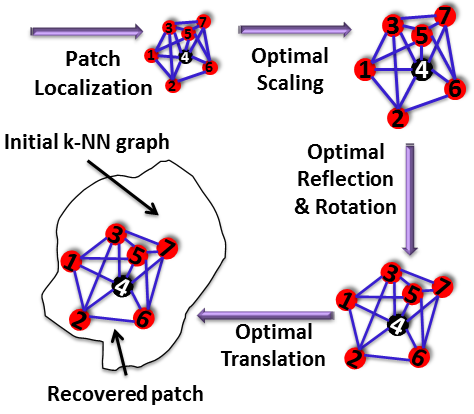
Fig. 1: ASAP and scale synchronization pipeline.

3.4 Extension to higher dimensions

Although we present experiments here on 2D and 3D data, the ASAP approach extends naturally to higher dimensions. In the 3D case, ASAP has been recently used as a scalable robust approach to the molecule problem in structural biology [36]. For the $d$-dimensional general case, one can extend ASAP by first using the same approach for scaling synchronization from Section 3.2, then synchronizing over O($d$), and finally estimating the optimal translations over $R^{d}$ by solving $d$ overdetermined systems of linear equations via least-squares. The LOE approach that can be used to obtain the local patch embeddings required by ASAP, has a natural extension to the $d$-dimensional case, thus rendering the entire pipeline amenable to dealing with higher-dimensional data.

4 Density Estimation

In this section, we remark on the explicit connection between the graph embedding problem considered in this paper and the density estimation problem. In particular, one may approach the problem of recovering the unknown coordinates underlying the kNN graph by first aiming to estimate the density function that generates the coordinates. Suppose for example that one is able to estimate the pointwise density $u:\Omega\subseteq\mathbb{R}^{d}\rightarrow[0,1]$, up to some constant multiple, evaluated at each vertex of the graph, $x_{i}$. Next, as outlined in [2], one can assign weights to the originally unweighted kNN graph, defined by $w(x_{i},x_{j})=(u^{-1/d}(x_{i})+u^{-1/d}(x_{j}))/2$. Furthermore, it can be shown that the shortest path distance in the resulting weighted kNN graphs converges to the Euclidean distance of the original points as the number of points increases. In other words, applying multidimensional scaling to the shortest path distances on the weighted kNN graph will yield increasingly accurate embeddings of the original points $\{x_{i}\}_{i=1}^{n}$ as $n\rightarrow+\infty$.

In contrast to finding an approximate embedding from a density estimate, under certain conditions, the reverse process is also straightforward. With sufficiently many points and sufficiently strong priors on the distribution, the methodology of Maximum Penalized Likelihood Estimation (MPLE) applies [37]. One first assumes that the locations correspond to points drawn independently identically distributed according to some unknown underlying spatial distribution. MPLE approximates the most likely spatial distribution given the points observed and some assumed prior distribution on the space of distributions. The data fidelity term comes in the form of a log-likelihood term, a function of the distribution estimate and the point locations, and is given by

$$L(u,\{x_{i}\}_{i=1}^{n})=\sum_{i=1}^{n}\log(u(x_{i})),$$

and the penalty term, $P(u)$ enforces the prior distribution on the space of distributions. Typical choices for $P(u)$ include the $H^{1}$-seminorm regularizer, $P(u)=\frac{\lambda}{2}\int_{\Omega}|\nabla u|^{2}dx$, enforcing smoothness, and Total Variation (TV) norm regularization, $P(u)=\lambda\int_{\Omega}|\nabla u|dx$, which enforces smoothness, but also allows for edges. Therefore, general MPLE seeks to optimize the following energy over all probability distributions on the spatial domain $\Omega\subseteq\mathbb{R}^{d}$

$$\hat{u}=\mbox{argmax}_{u\geq 0,\int_{\Omega}udx=1}{L(u,\{x_{i}\}_{i=1}^{n})-P(u)}.$$

The form and scale of $P$ encodes different types and amounts of regularity in the resulting density estimate $u$. In practical settings, cross-validation should be performed to determine the appropriate amount of regularity to impose on a given data set.

For the purpose of using kNN graphs to recover densities, we will include a post-processing step for a subset of the embedding experiments, to which we apply a standard implementation of TV MPLE [38] to the embedded points. TV is a good choice of penalty because we will be applying it to points that are drawn from a piecewise constant density. The good density estimates based on good embeddings shown in Section 5 illustrate that there is in fact a strong connection between the embedding and density estimation problems.

The actual implementation of the TV MPLE relies on the Split Bregman (equivalently Alternating Direction Method of Multipliers) minimization technique in which one introduces a splitting and equality constraints that are enforced by performing saddle-point optimization of the augmented Lagrangian. This results in an iterative update procedure given by Algorithm 2.

Algorithm 2 TV MPLE

INPUT : $\{x_{i}\},\rho,\gamma$
$y=0,z=0$
For $numberIterations$ $\{\\$

$$\left(\hat{u},\hat{d}\right)=$$

$$\mbox{argmin}_{u\geq 0,d}\bigg{\{} \|d\|_{1}-\sum_{i=1}^{n}\log(u(x_{i}))$$

$$+\frac{\rho}{2}\|\nabla u-d+y\|_{2}^{2}+\frac{\gamma}{2}\left(\|u\|_{1}-1+z\right)^{2}\bigg{\}}$$

$$y= y+\tilde{\nabla}\hat{u}-\hat{d}$$

$$z= z+\|\hat{u}\|_{1}-1$$

$\}$

The first minimization step is actually replaced by minimizing over $u$, and $d$ individually, making use of the shrinkage proximal operator associated with the $\ell^{1}$ norm.

5 Experiments

Our experiments compare embeddings of points drawn from three different 2D synthetic densities: piecewise constant half-planes (PC), piecewise constant squares (PCS), and Gaussian (Gauss), and a 3D synthetic denisty : piecewise constant half-cubes (halfcube), each with $n=\{500,1000,5000\}$ points, as well as points drawn uniformly from a 3D donut shape (Donut) with $n=500$, and the actual 2D coordinates of $n=1101$ cities in the US (US cities). For a given set of data points, we use its kNN adjacency matrix as input to each ordinal embedding method. Separate from these datasets with a clear correct geometric embeddings, we find embeddings of points in a co-authorship network of network scientists (NetSci2010) with $n=552$ (see Section 5.6). We test Laplacian Eigenmaps [39], the LOE BFGS and LOE MM methods [18], and ASAP with LOE BFGS used for the patch embeddings. As LOE was already compared with several methods in [18], attaining better performance than LOE may suggest better performance than a number of relevant methods including Kamada and Kawai [40], and Fruchterman and Reingold [41]. We remark that our approach deals with a different input than that of the t-SNE method in [42], which is generally used for embeddings of high dimensional data where some of the constraints are deliberately violated, which is not necessarily the case in our setting. We evaluate the methods based on (wall-clock) runtime and two different error metrics, Procrustes alignment error[43], and A-error ($\mathcal{E}_{A}$) defined as the percentage of edge disagreements between the kNN adjacency matrix of the proposed embeddeding $\tilde{X}$ and the ground truth

$$\mbox{error}(\tilde{X},X):\;\;\mathcal{E}_{A}\;\;\stackrel{{\scriptstyle\mathclap{\small\mbox{def}}}}{{=}}\;\;\frac{1}{n^{2}}\sum_{i,j=1}^{n}\left|\left(A^{k}_{\tilde{X}}\right)_{ij}-\left(A^{k}_{X}\right)_{ij}\right|,$$ (7)

where $A_{X}^{k}\in\{0,1\}^{n\times n}$ denotes the adjacency matrix of the corresponding kNN graph. We set varying limits on the number of LOE iterations $\{5,10,50,100,300,500\}$, and we use varying maximum patch sizes (MPS) for ASAP . The LOE and ASAP methods give, for each distribution and values $n$ and $k$, an error-runtime Pareto curve (with low values in both coordinates being best). In Table 1, we establish some shorthand notation for the methods and parameters used in this section. For fair comparisons, we pass the same randomly sampled data to each of the methods. Ideally, one would run these experiments many times over and average the results (to get an estimate of average performance), but this is effect already partially accomplished by running the LOE and ASAP methods with multiple parameters to get a more holistic measurement of performance. It is worth mentioning that while LOE BFGS and LOE MM are iterative methods which should converge to the best estimate of the solution as the number of iterations increases, ASAP is not iterative and the results of ASAP LOE with a given MPS, do not inform the results of ASAP LOE with another MPS. This aspect, combined with the randomized k-means spectral clustering used to choose patches means that we do not generally expect the recovery errors of ASAP LOE to be monotonically decreasing with MPS or time (as higher MPS generally leads to longer computational time). A principled way of choosing the best MPS for a given application of ASAP LOE could be of further interest.

Recovery Method
LE	Laplacian Eigenmaps embedding
LOE MM	Local Ordinal Embedding using majorization minimization
LOE BFGS	Local Ordinal Embedding using BFGS
ASAP LOE	ASAP & LOE BFGS patch embeddings
Parameters
sparse k	$k=\lceil 2\log(n)\rceil$
dense k	$k=\lceil\sqrt{n\log(n)}\rceil$
MPS	maximum patch size (for ASAP)
Iter.	number of iterations (of LOE)
Data sets
PC	2D piecewise constant half-planes
PCS	2D piecewise constant squares
Gauss	2D Gaussian
halfcube	3D piecewise constant half-cubes
Donut	3D Donut
US cities	2D coordinates of US cities
NetSci2010	co-authorship network of scientists

Table 1: Notation for plotting experimental results.

5.1 The need for scale synchronization

First, to illustrate the importance of the scale synchronization introduced in Section 3.2, we compare in Figure 2 ASAP synchronized embeddings with and without this step. Clearly, this step significantly improves the recovered solutions.

Fig. 2: Left: Ground truth, $n=1000,k=14$. Middle: ASAP LOE with scale synchronization: $\mathcal{E}_{A}=0.007$. Right: ASAP LOE without scale synchronization: $\mathcal{E}_{A}=0.038$.

5.2 Simulations with $n=500,1000,5000$ with sparse and dense $k$

We show $\mathcal{E}_{A}$ versus runtime for recovering $n=\{500,1000,5000\}$ points sampled from the PC (Figure 3), PCS (Figure 4), and Gaussian (Figure 5), with each figure showing results in the sparse and dense $k$ regime (see Table 1). We also show $\mathcal{E}_{A}$ versus runtime for $n=\{500,1000,5000\}$ points drawn from the halfcube (Figure 6) distribution for $k=50,150250,450$. Even for lower values of $n$, we find that ASAP LOE is often either faster than or better-performing than LOE BFGS, or both. This seems to be especially true in the sparse $k$ domain. This is partly due to the massively parallel embedding step in ASAP, which can take advantage of multiple cores as the problem scales. One would expect that as $n$ continues to grow, if more processors are made available and memory increases sufficiently, the advantage of embedding parallelization would continue to increase.

Fig. 3: $\mathcal{E}_{A}$ vs. time, $n=\{500,1000,5000\}$, Left : $k$ sparse, Right : $k$ dense, piecewise constant half-planes, $\boldsymbol{\circ}$ ASAP LOE, $\boldsymbol{\times}$ LOE BFGS, $\boldsymbol{\square}$ LE , $\boldsymbol{\star}$ LOE MM

Fig. 4: $\mathcal{E}_{A}$ vs. time, $n=\{500,1000,5000\}$, Left : $k$ sparse, Right : $k$ dense, piecewise constant half-planes, $\boldsymbol{\circ}$ ASAP LOE, $\boldsymbol{\times}$ LOE BFGS, $\boldsymbol{\square}$ LE , $\boldsymbol{\star}$ LOE MM

Fig. 5: $\mathcal{E}_{A}$ vs. time, $n=\{500,1000,5000\}$, Left : $k$ sparse, Right : $k$ dense, Gaussian density $\boldsymbol{\circ}$ ASAP LOE, $\boldsymbol{\times}$ LOE BFGS, $\boldsymbol{\square}$ LE , $\boldsymbol{\star}$ LOE MM

Fig. 6: $\mathcal{E}_{A}$ vs. time, $n=\{500,1000,5000\}$, $k=50,150,250,450$, 3D half-cube density $\boldsymbol{\circ}$ ASAP LOE, $\boldsymbol{\times}$ LOE BFGS, $\boldsymbol{\square}$ LE , $\boldsymbol{\star}$ LOE MM

To further illustrate how the methods perform, we plot the embeddings of $n=1000$ point sampled from the 2D densities in Figure 7. In each case, the ASAP LOE with MPS=400 takes less time to run and yields smaller $\mathcal{E}_{A}$ errors than the LOE BFGS with 100 maximum iterations. We only run LOE MM for $n=500$ because of difficulties we had when trying to get the provided R implementation to run on our Linux-based remote computing resource. We ran into no problems with the LOE BFGS implementation. The computers used have 12 CPU cores which are Intel(R) Xeon(R) X5650 @ 2.67GHz, and have 48GB ram. The R implementation of LOE does not (as far as its authors are aware) take advantage of multiple cores, and runs a single process on a single core. In contrast, our ASAP Matlab implementation uses the Multicore package to divide up the local embedding problems among the available cores.

Fig. 7: Embeddings for the PC (left), PCS (middle), and Gauss (right) data sets with $n=1000$, and $k$ dense. Row 1 : LE. Row 2: LOE BFGS Iter.=100. Row 3: ASAP LOE with MPS = 400 (with each ASAP result obtained is less time than the corresponding LOE result). Row 4: ground truth.

Fig. 8: Embeddings for halfcube data sets with $n=1000$, and $k=50$ (left), 150 (middle), 450 (right) Row 2: LOE BFGS Iter.=100. Row 3: ASAP LOE with MPS = 300 (with each ASAP result obtained is less time than the corresponding LOE result). Row 4: ground truth.

Fig. 9: Embeddings of Donut (3D) and US Cities (2D) data sets. Row 1: LOE BFGS Iter.=500. Row 2: ASAP LOE MPS=300 (with each ASAP result obtained in less time than the corresponding LOE result). Row 3: Ground truth.

To demonstrate that this approach is not limited to the 2D case, nor does it only perform well on synthetic data, we plot in Figure 9 the embeddings Procrustes aligned with points sampled from a 3D donut shape, and actual coordinates of $n=1101$ US cities. In both cases, ASAP LOE with MPS=300 runs faster and yields smaller $\mathcal{E}_{A}$ than LOE BFGS with 500 maximum iterations, the latter of which produces twisted or folded results.

5.3 Large $n$ : 50,000

In Table 2 we show $\mathcal{E}_{A}$ vs runtime for ASAP LOE on a data set of $n=50,000$ points and $k=22$. While this size is completely prohibitive for LOE BFGS, ASAP LOE produces good results in less than 4 hours. The worst possible result would be all edges of original graph misplaced, meaning $\mathcal{E}_{A}=2\cdot 50k\cdot 22/(50k)^{2}=8.8\times 10^{-4}$. $\mathcal{E}_{A}=2\times 10^{-4}$ means we get approximately $3/4$ of the edges correct.

MPS	100	300	500
PCS $\mathcal{E}_{A}$	$5.1\times 10^{-4}$	$5.6\times 10^{-4}$	$1.9\times 10^{-4}$
PC $\mathcal{E}_{A}$	$5.8\times 10^{-4}$	$4.7\times 10^{-4}$	$3.0\times 10^{-4}$

Table 2: Recovery results for $n=50,000$ for ASAP LOE.

5.4 Increasing $k$

We show in Figure 10, scaled $(n/k)\times\text{NumberNonzero}(A-A_{0})$ (this is a rescaling of $\mathcal{E}_{A}$ proportional to number of misplaced edges, more comparable for different values of $k$) and procrustes error versus increasing values of $k$ for $n=\{5000\}$ points drawn from the piecewise constant half-planes distribution using the method ASAP LOE with MPS=300. We see that for large $n$, adjacency matrix error and Procrustes error remain relatively small and stable over a range of small increasing $k$. Additionally, we show in Figure 16 some of the embeddings corresponding to these results. Like the Procrustes error plot, these embeddings suggest that for a range of $k$ small relative to $n$ and not too large relative to MPS, ASAP LOE BFGS returns sensible, although not perfect results. As $k$ gets too large however the results are quite poor. We suspect this is a result of $k$ being too large relative to MPS, leading to patches which are overly dense. When an ordinal graph contains nearly all possible edges, it essentially provides no information. When such data is of specific interest, one could either increase the mps as computational resources and time allow, or potentially use an alternate method for breaking the graph into overlapping patches which are not too dense.

Fig. 10: ASAP LOE MPS=300, $n=5000$, $k$ increasing by 20, Left: number of differences in adjacency matrix divided by number of edges, $nk$, Right: Procrustes error.

5.5 Density Estimation Experiments

In Figure 11 we show the results of applying TV MPLE to some of the embeddings shown in Figure 7. The regularization parameter used is .0001 . This is not obtained by cross-validation, but it simply seems to perform well on the originally sampled points. The densities of the approximate embeddings are as expected, with ASAP LOE BFGS recovering the density best, with LOE BFGS behind, and LE doing the worst. This altogether suggests that better embedding results do lead to better density estimation, if that is the end goal.

Fig. 11: TV MPLE applied to example embeddings of PC $n=1000$, $k$ dense, and top left : LE, top right : LOE BFGS maxIt=100, bottom left : ASAP LOE BFGS max patch size 400, bottom right : estimated density from ground truth points, see column 1 of Figure 7

Fig. 12: TV MPLE applied to example embeddings of PCS $n=1000$, $k$ dense, and top left : LE, top right : LOE BFGS maxIt=100, bottom left : ASAP LOE BFGS max patch size 400, bottom right : estimated density from ground truth points, see column 2 of Figure 7

5.6 Network of network scientists embedding

To further illustrate potential of ordinal embedding to broad categories of data, we present here an experiment embedding data that does not have an apparent ground-truth geometry. We use data from a co-authorship network of network scientists [44] from 2010, which was studied in [45] to evaluate methods of computing core-periphery structure. The network contains nonegatively weighted undirected edges where the weights are based on the number of papers they have co-authored. The network has 552 nodes and 1318 edges, with the number of edges attached to each node ranging from 1 to 38. The mean number of edges attached to each node is 4.7754 and the median is 4.

To embed the data, we treat the co-authorship links as nearest neighbor relationships. In other words, if X and Y have authored papers together, but X has not authored any papers with Z, we impose that the distance between X and Y should be smaller than the distance between X and Z. We used LOE BFGS and ASAP LOE BFGS to perform these embeddings in 2D and 3D. In this case, the LOE results were ultimately best with the 2D LOE BFGS 500 iteration embedding misplacing 754 of the 1318 nearest neighbor edges and the 3D LOE BFGS 500 Iteration embedding misplacing 272 of the nearest neighbor edges, while the 2D ASAP LOE BFGS mps 500 misplaced 910 edges, and the 3D ASAP LOE BFGS mps 500 misplaced 467 edges. That being said, several of the runtimes for the ASAP LOE results beat the LOE results. We speculate that the reasons LOE outperforms ASAP LOE in accuracy in this case are twofold : 1) the number of nodes, $n=552$, is too small to make the LOE method applied to the full data sufficiently intensive, and 2) the wide distribution of degrees of the nodes in the network perhaps does not go well with our approach of breaking up the network via spectral clustering. Perhaps other methods for braking up the network should be considered when the degree distribution is highly varied.

Independent of the comparison of the two methods, we look at the best 2D and 3D embeddings from LOE (shown in Figure 13 and Figure 14 respectively), to see if the embeddings preserve any interesting structure in the network. Since the network was previously studied for core-periphery detection, we color the nodes based on the corescore computed by the method proposed in [45] (mapping low values to blue and high values to red), and label the names of the authors with the top 10 corescores. These red, core authors appear primarily central to the embeddings, suggesting that these embeddings preserve important structural properties in the original network.

Fig. 13: LOE BFGS 2d embeddings of data from NetSci2010 data set, $n=552$, where co-authorship imposes that authors should be close

Fig. 14: LOE BFGS 3d embeddings of data from NetSci2010 data set, $n=552$, where co-authorship imposes that authors should be close

6 A Linear Program Alternative to SDP embedding

In this section we present the algorithm and a few results for a Linear Program Embedding approach using metric MDS (LPEm) for ordinal embedding. Though the results are ultimately not competitive with Local Ordinal Embedding, the approach is different enough so that the ideas may be of independent interest. In contrast to the SDP methods which cast embedding problems in terms of the Gram matrix $K$ our LPEm approach for kNN embedding optimizes over the variables $D$ (the distance matrix), $R$ (the radius at each node), and the slack variables. The radius at each node $i$, denoted by $R_{i}$ is defined to be the distance between node $i$ and its $k$-th closest neighbor. Thus $R_{i}$ is the radius of the neighborhood at node $i$. In kNN embedding, the objective and constraints can be written as linear constraints in $D,R$ and the slack variables, altogether leading to a linear program which is computationally cheaper to solve than an SDP. Although SDP-based methods can encompass a larger class of problems, they currently do not approach the scalability or numerical maturity of LP and SOCP solvers.

After the LP returns a candidate distance matrix $D$ and radii $R$, we pass $D$ into a standard mdscale, here using metric multidimensional scaling (see Algorithm 3),

$$(D^{*},R^{*})= \underset{\alpha,\beta,R,D}{\mbox{argmin}} \sum_{ij\in E(G)}\alpha_{ij}+\sum_{ij\notin E(G)}\beta_{ij}$$

subject to $$\alpha,\beta\in\mathbb{R}_{+}^{n\times n},R\in\mathbb{R}_{+}^{n},D\in\mathbb{R}_{+,sym}^{n\times n}$$

$$D_{ij}\leq R_{i}+\alpha_{ij},\mbox{ if }ij\in E(G)$$

$$D_{ij}>R_{i}-\beta_{ij},\mbox{ if }ij\notin E(G)$$

$$\sum_{i=1}^{n}R_{i}=V$$

$$D_{ij}+D_{ik}\leq D_{kl},(i,j,k)\in\mathcal{T}$$

$$X= \mbox{mds}\left(D^{*},d\right)$$

Algorithm 3 LP approach

where by $\mathcal{T}$ we mean the set of triangle inequalities we considered (ordered set $(i,j,k)$). If $(i,j,k)\in\mathcal{T}$, the same holds true for the two other permutations. The full set of triangle inequalities are necessary, though not sufficient, for the matrix $D$ to correspond to an Euclidean distance matrix. If one omits slack variables, there are $n(n-1)/2$ distance values to solve for along with $n$ radii, and thus $n(n+1)/2$ unknowns in total. Considering the ordinal constraints, for the upper bounds on the entries $D_{ij}$, there are $n$ ways to choose $i$, and for each $i$ there are $k$ ways to choose $j$, thus $nk/2$ constraints (accounting for symmetric distances). For the lower bounds on the entries $D_{ij}$ there are $n$ ways to choose $i$ and for each $i$ there are $n-k-1$ ways to choose $j$, giving $n(n-k-1)/2$ constraints. So there are $n(n-1)/2$ ordinal constraints on relating the $n(n-1)/2$ distances and $n$ radii. In other words, the intuition behind the added triangle inequalities is that they help to better constrain the system. There are on the order of $n^{3}$ triangle inequalities (choose any three points), so for large $n$, there are many more constraints than unknowns.

To avoid the added complexity from imposing all triangle inequalities, one could consider models that impose only a fraction of such constraints via either imposing them locally, for $k$-hop neighboring triples of points, or globally, such as picking edges via an Erdős-Rényi model, or mixing the two approaches.

We remark that dropping triangle inequalities altogether could certainly speed up the embedding process. The resulting non-metric $D$ may correspond to an increasing function of distance (e.g., distance squared), which suggests that non-metric MDS would be appropriate.

In general, even if the recovered distance metric corresponds to a metric distance, this is not a guarantee that the distance is realizable in a low-dimensional space. That requires a rank constraint on $D$, which is non-convex and is computationally intractable for an LP or SDP. The ultimate embedding into a low-dimensional space thus potentially gives up some structure in both the LP and SDP formulation, and it can be argued that this effect is lessened via the local to global approach.

In Figure 15 we show an example with points drawn from the densities discussed in the previous section along with points embedded using the LPEm approach. In these experiments we use a very dense value of $k$, $k=n/2=50$, which is where the approach seemed to work the best. The recovery of the piecewise constant half-planes is the best, but the preliminary results led us to decide not to experiment with this method further for the time being. The method was implemented using the CVX library, a package for specifying and solving convex programs ([46, 47]). Overall, we find the LP formulation appealing due to its simplicity. It would be interesting if a similarly simple approach could obtain competitive results on the problem of ordinal embedding, especially since until the work of von Luxburg and Alamgir [2], it was unknown to the community whether the problem was practically solvable at all.

Fig. 15: Linear Program Embeddings for the PC (left), PCS (middle), and Gauss (right) data sets with $n=100$, Row 1 : $k=22$ Row 2: $k=50$ Row 3: ground truth. Line segments highlight the displacement of each point.

7 Summary and discussion

We have demonstrated that the computational efficiency of LOE for the kNN embedding problem can be significantly improved, while maintaining and often improving spatial and ordinal accuracy in a distributed setting. Our application of the divide-and-conquer ASAP method renders the problem of kNN embedding significantly more tractable, distributing the embedding steps, and using fast spectral methods to combine them. We expect that such improvements will make it possible to use kNN embeddings in a broader range of settings, and that the ASAP framework will be of independent interest to the machine learning community for tackling large geometric embedding problems.

Fig. 16: ASAP LOE BFGS MPS=300, $n=5000$, $k$ increasing by 20, Top left : originally sampled points, Remaining plots : recovered embeddings

References

- [1] S. Agarwal, J. Wills, L. Cayton, G. Lanckriet, D. J. Kriegman, and S. Belongie, “Generalized non-metric multidimensional scaling,” in AISTATS, 2007, pp. 11–18.
- [2] U. von Luxburg and M. Alamgir, “Density estimation from unweighted k-nearest neighbor graphs: a roadmap,” in NIPS, 2013, pp. 225–233.
- [3] R. N. Shepard, “The analysis of proximities: Multidimensional scaling with an unknown distance function i,” Psychometrika, vol. 27, no. 2, pp. 125–140, 1962.
- [4] J. B. Kruskal, “Multidimensional scaling by optimizing goodness of fit to a nonmetric hypothesis,” Psychometrika, vol. 29, no. 1, pp. 1–27, 1964.
- [5] J. B. Kruskal, “Nonmetric multidimensional scaling: a numerical method,” Psychometrika, vol. 29, no. 2, pp. 115–129, 1964.
- [6] B. Shaw and T. Jebara, “Structure preserving embedding,” in ICML. ACM, 2009, pp. 937–944.
- [7] B. McFee and G. R. Lanckriet, “Partial order embedding with multiple kernels,” in ICML, 2009, pp. 721–728.
- [8] M. Quist and G. Yona, “Distributional scaling: An algorithm for structure-preserving embedding of metric and nonmetric spaces,” The Journal of Machine Learning Research, vol. 5, pp. 399–420, 2004.
- [9] O. Tamuz, C. Liu, S. Belongie, O. Shamir, and A. T. Kalai, “Adaptively learning the crowd kernel,” arXiv preprint arXiv:1105.1033, 2011.
- [10] K. G. Jamieson and R. D. Nowak, “Low-dimensional embedding using adaptively selected ordinal data,” in Communication, Control, and Computing (Allerton). IEEE, 2011, pp. 1077–1084.
- [11] R. Rosales and G. Fung, “Learning sparse metrics via linear programming,” in Proceedings of the 12th ACM SIGKDD international conference on knowledge discovery and data mining. ACM, 2006, pp. 367–373.
- [12] N. Ailon, “Active learning ranking from pairwise preferences with almost optimal query complexity.,” in NIPS, 2011, pp. 810–818.
- [13] H. Ouyang and A. Gray, “Learning dissimilarities by ranking: from sdp to qp,” in ICML. ACM, 2008, pp. 728–735.
- [14] B. McFee and G. R. Lanckriet, “Metric learning to rank,” in ICML, 2010, pp. 775–782.
- [15] K. G. Jamieson and R. D. Nowak, “Active ranking using pairwise comparisons.,” in NIPS, 2011, vol. 24, pp. 2240–2248.
- [16] Y. Lan, J. Guo, X. Cheng, and T.-Y. Liu, “Statistical consistency of ranking methods in a rank-differentiable probability space.,” in NIPS, 2012, pp. 1241–1249.
- [17] F. Wauthier, M. Jordan, and N. Jojic, “Efficient ranking from pairwise comparisons,” in Proceedings of the 30th International Conference on Machine Learning, 2013, pp. 109–117.
- [18] Y. Terada and U. V. von Luxburg, “Local ordinal embedding,” in ICML, 2014, pp. 847–855.
- [19] D. S. H. Martinez, M. Gonzalez, X. Huang, B. Irvine, C. H. Hsieh, Y. R. Huang, M. B. Short, and A. L. Bertozzi, “An economical testbed for cooperative control and sensing strategies of robotic micro-vehicles,” in Informatics in Control, Automation and Robotics, pp. 65–75. Springer, 2013.
- [20] M. Gonzalez, X. Huang, D. S. H. Martinez, C. H. Hsieh, Y. R. Huang, B. Irvine, M. B. Short, and A. L Bertozzi, “A third generation micro-vehicle testbed for cooperative control and sensing strategies.,” in ICINCO (2), 2011, pp. 14–20.
- [21] M. Cucuringu, Y. Lipman, and A. Singer, “Sensor network localization by eigenvector synchronization over the Euclidean group,” ACM Trans. Sen. Netw., vol. 8, no. 3, pp. 19:1–19:42, Aug. 2012.
- [22] U. von Luxburg and M. Kleindessner, “Uniqueness of ordinal embedding,” in COLT, 2014, pp. 40–67.
- [23] W. S. Torgerson, Theory and methods of scaling., Wiley, 1958.
- [24] J. B. Kruskal and M. Wish, Multidimensional scaling, vol. 11, Sage, 1978.
- [25] K. Toh, P. Biswas, and Y. Ye, “SNLSDP- a MATLAB software for sensor network localization,” October 2008.
- [26] D. Shamsi, N. Taheri, Z. Zhu, and Y. Ye, “On Sensor Network Localization Using SDP Relaxation,” ArXiv e-prints, Oct. 2010.
- [27] K. Q. Weinberger and L. K. Saul, “An introduction to nonlinear dimensionality reduction by maximum variance unfolding,” in AAAI, 2006, vol. 6, pp. 1683–1686.
- [28] Y. Gao and D. F. Sun, “A majorized penalty approach for calibrating rank constrained correlation matrix problems,” 2010.
- [29] P. Biswas and Y. Ye, “Semidefinite programming for ad hoc wireless sensor network localization,” in Proceedings of the Third International Symposium on Information Processing in Sensor Networks, New York, 2004, pp. 46–54, ACM.
- [30] P. Biswas, T. C. Lian, T. C. Wang, and Y. Ye, “Semidefinite programming based algorithms for sensor network localization,” ACM Transactions on Sensor Networks, vol. 2, no. 2, pp. 188–220, 2006.
- [31] P. Biswas, T. Liang, K. Toh, Y. Ye, and T. Wang, “Semidefinite programming approaches for sensor network localization with noisy distance measurements,” IEEE Transactions on Automation Science and Engineering, vol. 3, no. 4, pp. 360–371, 2006.
- [32] P. Biswas, H. Aghajan, and Y. Ye, “Semidefinite programming algorithms for sensor network localization using angle of arrival information,” in Proc. 39th Annu. Asilomar Conf. Signals, Systems, and Computers, Oct. 2005, pp. 220–224.
- [33] Z. Zhu, A. M. C. So, and Y. Ye, “Universal rigidity: Towards accurate and efficient localization of wireless networks,” in Proc. IEEE INFOCOM, 2010.
- [34] A. Singer, “Angular synchronization by eigenvectors and semidefinite programming,” Appl. Comput. Harmon. Anal., vol. 30, no. 1, pp. 20–36, 2011.
- [35] U. von Luxburg, “A tutorial on spectral clustering,” Statistics and computing, vol. 17, no. 4, pp. 395–416, 2007.
- [36] M. Cucuringu, A. Singer, and D. Cowburn, “Eigenvector synchronization, graph rigidity and the molecule problem,” Information and Inference, vol. 1, no. 1, pp. 21–67, 2012.
- [37] Paulus Petrus Bernardus Eggermont and Vincent N LaRiccia, Maximum Penalized Likelihood Estimation: Regression, vol. 2, Springer, 2001.
- [38] George O Mohler, Andrea L Bertozzi, Thomas A Goldstein, and Stanley J Osher, “Fast tv regularization for 2d maximum penalized likelihood estimation,” Journal of Computational and Graphical Statistics, vol. 20, no. 2, pp. 479–491, 2011.
- [39] M. Belkin and P. Niyogi, “Laplacian eigenmaps for dimensionality reduction and data representation,” Neural Computation, vol. 15, no. 6, pp. 1373–1396, June 2003.
- [40] T. Kamada and S. Kawai, “An algorithm for drawing general undirected graphs,” Information processing letters, vol. 31, no. 1, pp. 7–15, 1989.
- [41] T. M. J. Fruchterman and E. M Reingold, “Graph drawing by force-directed placement,” Software: Practice and experience, vol. 21, no. 11, pp. 1129–1164, 1991.
- [42] L. Van der Maaten and K. Weinberger, “Stochastic triplet embedding,” in IEEE Workshop on Machine Learning for Signal Processing (MLSP), 2012, pp. 1–6.
- [43] R. Sibson, “Studies in the robustness of multidimensional scaling: Procrustes statistics,” Journal of the Royal Statistical Society. Series B, pp. 234–238, 1978.
- [44] D. Edler and M. Rosvall, “The mapequation,” http://www.mapequation.org, software package, available online.
- [45] M Puck Rombach, Mason A Porter, James H Fowler, and Peter J Mucha, “Core-periphery structure in networks,” SIAM Journal on Applied mathematics, vol. 74, no. 1, pp. 167–190, 2014.
- [46] Michael Grant and Stephen Boyd, “CVX: Matlab software for disciplined convex programming, version 2.1,” http://cvxr.com/cvx, Mar. 2014.
- [47] Michael Grant and Stephen Boyd, “Graph implementations for nonsmooth convex programs,” in Recent Advances in Learning and Control, V. Blondel, S. Boyd, and H. Kimura, Eds., Lecture Notes in Control and Information Sciences, pp. 95–110. Springer-Verlag Limited, 2008, http://stanford.edu/~boyd/graph_dcp.html.
- [48] R. Connelly and W. J. Whiteley, “Global rigidity: The effect of coning,” Discrete and Computational Geometry, 2009.
- [49] Steven J. Gortler, Alexander D. Healy, and Dylan P. Thurston, “Characterizing generic global rigidity,” AMERICAN JOURNAL OF MATHEMATICS, vol. 4, pp. 897, 2010.
- [50] B. Hendrickson, “Conditions for unique graph realizations,” SIAM J Comput, vol. 21, pp. 65–84, 1992.
- [51] B. Roth, “Rigid and flexible frameworks,” The American Mathematical Monthly, vol. 88, pp. 6–21, 1981.
- [52] H. Gluck, “Almost all simply connected closed surfaces are rigid,” Geometric Topology, Lecture Notes in Mathematics, vol. 438, pp. 225–239, 1975.
- [53] L. Asimow and B. Roth, “The rigidity of graphs,” Trans. Amer. Math. Soc., vol. 245, pp. 279–289, 1978.
- [54] R. Connelly, “On generic global rigidity,” Applied Geometry and Discrete Mathematics, vol. 4, pp. 147–155, 1991.
- [55] R. Connelly, “Generic global rigidity,” Discrete Comput. Geom, vol. 33, pp. 549–563, 2005.
- [56] Bill Jackson and Tibor Jordán, “Connected rigidity matroids and unique realizations of graphs,” Journal of Combinatorial Theory, Series B, vol. 94, no. 1, pp. 1–29, 2005.