$q$-randomized Robinson–Schensted–Knuth correspondences and random polymers

Abstract.

We introduce and study $q$-randomized Robinson–Schensted–Knuth (RSK) correspondences which interpolate between the classical ($q=0$) and geometric ($q\nearrow 1$) RSK correspondences (the latter ones are sometimes also called tropical).

For $0<q<1$ our correspondences are randomized, i.e., the result of an insertion is a certain probability distribution on semistandard Young tableaux. Because of this randomness, we use the language of discrete time Markov dynamics on two-dimensional interlacing particle arrays (these arrays are in a natural bijection with semistandard tableaux). Our dynamics act nicely on a certain class of probability measures on arrays, namely, on $q$-Whittaker processes (which are $t=0$ versions of Macdonald processes of Borodin–Corwin [7]). We present four Markov dynamics which for $q=0$ reduce to the classical row or column RSK correspondences applied to a random input matrix with independent geometric or Bernoulli entries.

Our new two-dimensional discrete time dynamics generalize and extend several known constructions: (1) The discrete time $q$-TASEPs studied by Borodin–Corwin [8] arise as one-dimensional marginals of our “column” dynamics. In a similar way, our “row” dynamics lead to discrete time $q$-PushTASEPs — new integrable particle systems in the Kardar–Parisi–Zhang universality class. We employ these new one-dimensional discrete time systems to establish a Fredholm determinantal formula for the two-sided continuous time $q$-PushASEP conjectured by Corwin–Petrov [23]. (2) In a certain Poisson-type limit (from discrete to continuous time), our two-dimensional dynamics reduce to the $q$-randomized column and row Robinson–Schensted correspondences introduced by O’Connell–Pei [59] and Borodin–Petrov [16], respectively. (3) In a scaling limit as $q\nearrow 1$, two of our four dynamics on interlacing arrays turn into the geometric RSK correspondences associated with log-Gamma (introduced by Seppäläinen [70]) or strict-weak (introduced independently by O’Connell–Ortmann [58] and Corwin–Seppäläinen–Shen [25]) directed random lattice polymers.

1. Introduction

1.1. Overview

The classical Robinson–Schensted–Knuth (RSK) correspondence associates to an integer matrix a pair of semistandard Young tableaux of the same shape [45], [35], [71], [68]. It is informative to view an integer matrix $M=(M_{ij})$ as a configuration of points (“balls”) in cells of the lattice $\mathbb{Z}_{\geq 0}^{2}$, with $M_{ij}$ balls in the $(i,j)$-th cell (see Fig. 1, left).

Figure 1. Left: an integer matrix as an input to the RSK. Center: an integer word as an input into the RS viewed as a matrix with the continuous $j$ coordinate (at most one ball at a given horizontal position is allowed; the word encodes vertical positions of consecutive balls). Right: a permutation viewed as a matrix with both continuous coordinates (at most one ball at a given horizontal or vertical position is allowed; balls represent the graph of the permutation).

There are also simpler correspondences obtained from the RSK if one makes one or both dimensions of the input continuous, see Fig. 1, center and right. In particular, the Robinson–Schensted (RS) correspondence maps integer words into pairs of Young tableaux of the same shape, but now one of them is standard.

The idea of applying the RSK correspondence to a random input can be traced back to [72] where it was used in connection with the asymptotic theory of characters of the infinite symmetric group (see also [17]). Together with combinatorial properties of the RSK this idea has been extensively employed in studying various stochastic systems, e.g., TASEP (= totally asymmetric simple exclusion process), the last-passage percolation [42], or longest increasing subsequences of random permutations [1], [2].

Reading the random input matrix column by column adds a dynamical perspective to random systems (with $j$ in all three cases on Fig. 1 playing the role of time). This direction has been substantially developed in, e.g., [54], [55], [5].

The geometric version (also sometimes called “tropical”) of the RS and the RSK correspondences has also been employed in the study of stochastic systems [56], [22], [60], [57]. The systems one obtains at this level are related to directed random polymers in random media, in particular, to the O’Connell–Yor, log-Gamma, and strict-weak random polymers introduced in [61], [70], and [58], [25], respectively. Each such polymer model can be viewed as a positive temperature version of a certain last-passage percolation-like model.

In the stochastic systems mentioned above, the RSK and related constructions provide a way to observe and understand their integrability. The integrability property refers to the presence of concise and exact formulas describing observables, which allows to study the asymptotic behavior of such systems, and also gives access to exact descriptions of limiting universal distributions, such as the Tracy-Widom distributions which are features of the Kardar–Parisi–Zhang (KPZ) universality class [20], [14], [15] [67].

The classical RSK is deeply connected to Schur symmetric functions [52, Ch. I], while the geometric RSK is relevant to the $\mathfrak{gl}_{n}$ Whittaker functions [49], [28]. Both families of functions are degenerations of more general Macdonald symmetric functions depending on two parameters $(q,t)$ [52, Ch. VI]: the Schur functions correspond to $q=t$, and the Whittaker functions arise in the limit as $t=0$ and $q\nearrow 1$, [38].

In the recent years, there has been a progress in understanding analogues of the RS correspondences at other levels of the Macdonald hierarchy: $q$-Whittaker ($t=0$ and $0<q<1$) [59], [65], [16] and Hall–Littlewood ($q=0$ and $0<t<1$) [18]. At these levels, the correspondences become randomized, that is, the image of a deterministic word (as on Fig. 1, center) is no longer a fixed pair of Young tableaux, but rather a random such pair. Because of this randomness, an appropriate language for describing the correspondences seems to be that of Markov dynamics on two-dimensional interlacing integer arrays (these arrays are in a natural bijection with semistandard tableaux, see Remark 1.1 below for more detail). The dynamics which are analogues of the RS correspondences evolve in continuous time according to the $j$ axis on Fig. 1, center. These dynamics act nicely on certain families of probability distributions on interlacing arrays, namely, the Macdonald processes [7].

The $q$-Whittaker level is relevant to integrable one-dimensional particle systems such as (continuous time) $q$-TASEP and the stochastic $q$-Boson system [69], [7], [12], [10], [29], and (continuous time) $q$-PushTASEP (= $q$-deformed pushing TASEP) [23]. In particular, continuous time Markov dynamics on interlacing arrays constructed in [59] and [16] are two-dimensional extensions of, respectively, the $q$-TASEP and the $q$-PushTASEP. That is, the latter one-dimensional processes are Markovian marginals of the dynamics on two-dimensional interlacing arrays.

In the present paper we advance further at the $q$-Whittaker level, and introduce four $q$-randomized RSK correspondences, or, in other words, four discrete time Markov dynamics on interlacing arrays which act nicely on $q$-Whittaker processes (these are Macdonald processes with $t=0$). These dynamics unify, generalize and extend all of the above RSK-type constructions:

$\bullet$ When $q=0$, our four $q$-randomized correspondences become usual or dual, row or column classical RSKs (four classical correspondences in total). The input matrix $M$ in the usual RSKs has $M_{ij}\in\{0,1,2,\ldots\}$, and in the dual RSKs one has $M_{ij}\in\{0,1\}$. When one takes $M_{ij}$ to be independent geometric (for usual) or Bernoulli (for dual) random variables and applies a suitable classical RSK, the shape of the resulting random Young diagram is distributed according to the Schur measure [63]. Similarly, our $q$-randomized correspondences applied to $q$-geometric or Bernoulli random inputs (note that the Bernoulli input needs not to be $q$-deformed) give rise to $q$-Whittaker distributed random Young diagrams. The latter property is an instance of “acting nicely” on $q$-Whittaker processes (see also (2.17) in §2 for more detail).

$\bullet$ In a limit from discrete to continuous time, our $q$-randomized RSKs turn into the (simpler) $q$-randomized RS correspondences introduced and studied in [59], [16].

$\bullet$ The two discrete time $q$-TASEPs (associated with $q$-geometric or Bernoulli random variables) studied by Borodin–Corwin [8] arise as one-dimensional marginals of our two “column” dynamics on interlacing arrays. In a similar way, our two “row” dynamics lead to discrete time $q$-PushTASEPs — new integrable particle systems in the KPZ universality class.

$\bullet$ In a scaling limit as $q\nearrow 1$, the dynamics on interlacing arrays associated with the $q$-geometric random input (these are two out of our four $q$-randomized RSK correspondences) converge to geometric (tropical) RSK correspondences. The latter correspondences (which are deterministic birational maps between arrays of positive reals) are relevant to the log-Gamma [70], [22], [60] and strict-weak [25] random lattice polymers.

In §1.2 below we describe one of our four dynamics in detail, and in §1.3 we briefly discuss other dynamics and results.

Figure 2. Left: An interlacing array $\boldsymbol{\lambda}$; we require that $\lambda^{(j)}_{i}\in\mathbb{Z}_{\geq 0}$. Right: A configuration of particles corresponding to an interlacing array of depth $N=5$ (right).

1.2. $q$-randomized row insertion with $q$-geometric input

Discrete time Markov dynamics (i.e., the $q$-randomized RSK correspondences) which we construct in the present paper live on the space of integer arrays $\boldsymbol{\lambda}$ (see Fig. 2). Neighboring levels of the array satisfy certain inequalities which we call the interlacing property (see (2.1) for the definition). Each level $\lambda^{(j)}=(\lambda^{(j)}_{1}\geq\ldots\geq\lambda^{(j)}_{j})$ of an array can be viewed as a partition (equivalently, a Young diagram [52, I.1]), so $\boldsymbol{\lambda}$ is a sequence of interlacing Young diagrams.

Figure 3. A semistandard Young tableau corresponding to the array on Fig. 2, right.

Remark 1.1.

Each $\boldsymbol{\lambda}$ can be also viewed as a semistandard Young tableau of shape $\lambda^{(N)}$ filled with numbers from $1$ to $N$. Here “semistandard” means that in this filling, numbers increase weakly along rows, and strictly down columns. Then each $\lambda^{(j)}$ is the portion of the semistandard tableau filled with numbers from 1 to $j$, see Fig. 3.

Let us now define the ($q$-randomized) operation of inserting a word $w=(1^{m_{1}}2^{m_{2}}\ldots N^{m_{N}})$ (i.e., the word has $m_{1}$ ones, $m_{2}$ twos, etc.) into an array $\boldsymbol{\lambda}$. The result is a new, random array $\boldsymbol{\nu}$. At the first level we have $\nu^{(1)}_{1}=\lambda^{(1)}_{1}+m_{1}$. Then, sequentially at all levels $j=2,\ldots,N$, given the existing change $\lambda^{(j-1)}\to\nu^{(j-1)}$ at the previous level and the old state $\lambda^{(j)}$ at the current level, construct the new state $\nu^{(j)}$ as follows. Each move $\nu^{(j-1)}_{i}-\lambda^{(j-1)}_{i}$, $i=1,\ldots,j-1$, is randomly split into two pieces $r_{i}^{(j-1)}+\ell_{i}^{(j-1)}$, and the piece $r_{i}^{(j-1)}$ is added to the new move of the upper right neighbor $\lambda^{(j)}_{i}$, while the piece $\ell_{i}^{(j-1)}$ is added to the new move of the upper left neighbor $\lambda^{(j)}_{i+1}$. Moreover, $\lambda^{(j)}_{1}$ receives an additional move of size $m_{j}$. All these splittings and moves at level $j$ happen in parallel. That is (here and below $\mathbf{1}_{\cdots}$ stands for the indicator),

$$\nu^{(j)}_{i}-\lambda^{(j)}_{i}=m_{j}\mathbf{1}_{i=1}+r_{i}^{(j-1)}\mathbf{1}_{i<j}+\ell_{i-1}^{(j-1)}\mathbf{1}_{i>1},\qquad i=1,\ldots,j$$

(see Fig. 4). To complete the definition, it now remains to describe the distribution of the splitting of the move $\nu^{(j-1)}_{i}-\lambda^{(j-1)}_{i}=r_{i}^{(j-1)}+\ell_{i}^{(j-1)}$. This is a certain $q$-deformed version of the Beta-binomial distribution, namely, $r_{i}^{(j-1)}$ is randomly chosen to be equal to $r\in\{0,1,2,\ldots,\nu^{(j-1)}_{i}-\lambda^{(j-1)}_{i}\}$ with probability

$$\boldsymbol{\varphi}_{q^{-1},q^{a},q^{b}}(r\mid c):=q^{ar}\frac{(q^{b-a};q^{-1})_{r}}{(q^{-1};q^{-1})_{r}}\frac{(q^{a};q^{-1})_{c-r}}{(q^{-1};q^{-1})_{c-r}}\frac{(q^{-1};q^{-1})_{c}}{(q^{b};q^{-1})_{c}},$$ (1.1)

where

$$a=\lambda^{(j)}_{i}-\lambda^{(j-1)}_{i},\qquad b=\lambda^{(j-1)}_{i-1}-\lambda^{(j-1)}_{i},\qquad c=\nu^{(j-1)}_{i}-\lambda^{(j-1)}_{i},$$

$(u;q)_{m}=(1-u)(1-uq)\ldots(1-uq^{m-1})$ are the $q$-Pochhammer symbols, and we adopt the convention $\lambda^{j-1}_{0}=+\infty$. The quantity $\ell^{(j-1)}_{i}$ is simply equal to $\nu^{(j-1)}_{i}-\lambda^{(j-1)}_{i}-r^{(j-1)}_{i}$.

The quantities (1.1) define a probability distribution in $r$ for $a\leq b$, $c\leq b$ (these conditions follow from the interlacing). Moreover, this distribution is supported on $\{0,1,\ldots,c\}\cap\{c-a,c-a+1,\ldots,b-a-1,b-a\}$, which in fact ensures that the new array $\boldsymbol{\nu}$ is also interlacing (see lemma 6.2 for details).

Figure 4. Splitting of the move at level $j-1$ and its propagation to the level $j$. Here we are using the particle interpretation of interlacing arrays as on Fig. 2, right.

Remark 1.2.

The interlacing array $\boldsymbol{\lambda}$ plays the role of the insertion tableau in our $q$-randomized RSK correspondence (cf. Remark 1.1). One can readily define an accompanying recording tableau in the same way as it is done for the classical RSK correspondences. In the present paper we will not focus on recording tableaux.

Now, let us take the insertion word $w=(1^{m_{1}}2^{m_{2}}\ldots N^{m_{N}})$ to be random itself. More precisely, let $m_{j}$, $j=1,\ldots,N$, be independent $q$-geometric random variables:

$$\operatorname{\mathrm{Prob}}(m_{j}=k)=\frac{\alpha^{k}}{(q;q)_{k}}(\alpha;q)_{\infty},\qquad k=0,1,2,\ldots,\qquad 0<\alpha<1.$$ (1.2)

Inserting this random word $w$ into an array $\boldsymbol{\lambda}$ defines one step of a discrete time Markov chain on interlacing arrays. We denote this Markov chain by $\mathscr{Q}^{q}_{\textnormal{row}}[\alpha]$.

Theorem 1.3.

Start the Markov dynamics $\mathscr{Q}^{q}_{\textnormal{row}}[\alpha]$ from the interlacing array with all $\lambda^{(j)}_{i}(0)=0$. Then the distribution of the array $\boldsymbol{\lambda}(T)$ after $T$ steps of this dynamics is given by the $q$-Whittaker process:

$$\operatorname{\mathrm{Prob}}(\boldsymbol{\lambda}(T)=\boldsymbol{\lambda})=(\alpha;q)^{TN}_{\infty}{P_{\lambda^{(1)}}(1)P_{\lambda^{(2)}/\lambda^{(1)}}(1)\ldots P_{\lambda^{(N)}/\lambda^{(N-1)}}(1)Q_{\lambda^{(N)}}(\underbrace{\alpha,\alpha,\ldots,\alpha}_{T})}.$$

Here $P_{\lambda/\mu}$ and $Q_{\lambda}$ are the $q$-Whittaker polynomials, see §2 for more detail. Theorem 1.3 follows from Theorem 6.4 which we prove in §6.2.

Remark 1.4.

In fact, we can (and will) consider a more general situation when the parameters $\alpha$ in (1.2) may depend on $j$ and on the time step as $\alpha_{t}a_{j}$. Then the $q$-Whittaker process above takes the form

$$\bigg{(}\prod_{j=1}^{N}\prod_{t=1}^{T}(\alpha_{t}a_{j};q)_{\infty}\bigg{)}{P_{\lambda^{(1)}}(a_{1})P_{\lambda^{(2)}/\lambda^{(1)}}(a_{2})\ldots P_{\lambda^{(N)}/\lambda^{(N-1)}}(a_{N})Q_{\lambda^{(N)}}(\alpha_{1},\alpha_{2},\ldots,\alpha_{T})}.$$

We omit the dependence on $j$ and $t$ in Introduction.

Let us now describe three degenerations of the dynamics $\mathscr{Q}^{q}_{\textnormal{row}}[\alpha]$:

$\bullet$ For $q=0$, the splitting distributions (1.1) become supported at a single $r\in\{0,1,\ldots,c\}$, so the randomness in the insertion disappears, and the insertion itself turns into the classical RSK row insertion (we recall its definition in §4.3). The $q$-geometric random variables $m_{j}$ (1.2) become geometric, and the $q$-Whittaker polynomials in Theorem 1.3 turn into the Schur polynomials. This justifies our treatment of the dynamics $\mathscr{Q}^{q}_{\textnormal{row}}[\alpha]$ as the $q$-randomized row RSK correspondences.

$\bullet$ Fix $0<q<1$. When $\alpha\searrow 0$ in (1.2) and one rescales time from discrete to continuous time (see §6.7 for details on this scaling), the random input matrix turns into $N$ independent Poisson processes running in parallel (i.e., we are passing from the left to the center situation on Fig. 1). Then in the splitting distributions one has $c=0$ or $1$, and the dynamics $\mathscr{Q}^{q}_{\textnormal{row}}[\alpha]$ turns into a continuous time dynamics on $q$-Whittaker processes which was introduced in [16]. The latter continuous time dynamics should be viewed as a $q$-randomized row RS correspondence.

$\bullet$ Let $q=e^{-\epsilon}$ and $\alpha=e^{-\theta\epsilon}$ with $\epsilon\searrow 0$ and $\theta>0$. Define the positive random variables $\hat{R}^{j}_{k}(t,\epsilon)$ via the following scaling:

$$\lambda^{(j)}_{k}(t)=(t+j-2k+1)\epsilon^{-1}\log\epsilon^{-1}+\epsilon^{-1}\log\big{(}\hat{R}^{j}_{k}(t,\epsilon)\big{)}.$$

If the quantities $\lambda^{(j)}_{k}$ evolve under the dynamics $\mathscr{Q}^{q}_{\textnormal{row}}[\alpha]$ started from all $\lambda^{(j)}_{k}(0)=0$, then the rescaled quantities $\hat{R}^{j}_{k}(t,\epsilon)$ converge to certain ratios of partition functions in the log-Gamma lattice polymer model (see §8.1 and Theorem 8.7 in particular for details). Moreover, under this scaling the randomness in the splitting (1.1) disappears, and the $q$-randomized insertion described above turns into the geometric RSK insertion.

Remark 1.5.

It is worth noting that there is also a strong connection between the geometric (tropical) RSK and representation theory, cf. [5], [19]. At the $q$-randomized level this connection does not (yet) seem to be present.

When restricted to the rightmost particles $\lambda^{(j)}_{1}$, $j=1,\ldots,N$, of the interlacing array, the dynamics $\mathscr{Q}^{q}_{\textnormal{row}}[\alpha]$ induces a marginally Markovian evolution which we call the (discrete time) geometric $q$-PushTASEP. This is a new integrable particle system in the KPZ universality class. In the shifted coordinates $x_{i}(t):=-\lambda_{1}^{(i)}(t)-i$ (so $x_{N}<\ldots<x_{1}$), the evolution of this system during time step $t\to t+1$ looks as follows. Sequentially for $i=1,2,\ldots,N$, each particle $x_{i}$ jumps to the left by $m_{i}+r^{(i-1)}_{1}$, where $m_{i}$ is an independent $q$-geometric random variable (1.2), and $r^{(i-1)}_{1}$ is a random variable with distribution

$$\boldsymbol{\varphi}_{q^{-1},q^{a},0}(r\mid c)=q^{ar}(q^{a};q^{-1})_{c-r}\frac{(q^{-1};q^{-1})_{c}}{(q^{-1};q^{-1})_{r}(q^{-1};q^{-1})_{c-r}},\qquad\begin{array}[]{l}a=x_{i-1}(t)-x_{i}(t)-1,\\ c=x_{i-1}(t+1)-x_{i-1}(t)\end{array}$$

(this is simply the splitting distribution (1.1) with $b=+\infty$). Note that if $c>a$, then $r^{(i-1)}_{1}$ chosen according to the above distribution will be at least $c-a$. See Fig. 5.

Figure 5. The discrete time geometric $q$-PushTASEP.

In a continuous time limit as $\alpha\searrow 0$, the geometric $q$-PushTASEP turns into the continuous time $q$-PushTASEP of [16], [23]. The $q$-moments of the form $\operatorname{\mathbb{E}}q^{k(x_{n}(t)+n)}$ (and more general such moments) of both $q$-PushTASEPs are given in terms of nested contour integrals. For the geometric $q$-PushTASEP only finitely many such moments exist (i.e., the expectation is infinite for sufficiently large $k$), and for the continuous time $q$-PushTASEP the moments grow too fast and also do not determine the distribution of $x_{n}(t)$. However, it is still possible to write down a Fredholm determinantal formula for the distribution of $x_{n}(t)$ for both processes (started from the step initial configuration $x_{i}(0)=-i$) using the theory of Macdonald processes [7], see [9, Theorem 3.3]. We refer to §7 for further details.

1.3. Other dynamics and results

Besides the dynamics $\mathscr{Q}^{q}_{\textnormal{row}}[\alpha]$ discussed in §1.2 above, we introduce three other dynamics on $q$-Whittaker processes:

$\bullet$ $\mathscr{Q}^{q}_{\textnormal{col}}[\alpha]$ (§6.4 and Theorem 6.11). At $q=0$ this dynamics becomes the classical RSK column insertion applied to a geometric random input $\mathscr{Q}^{q=0}_{\textnormal{col}}[\alpha]$ (§4.3). In a scaling limit as $q\nearrow 1$, $\mathscr{Q}^{q}_{\textnormal{col}}[\alpha]$ turns into a geometric (tropical) RSK associated with the strict-weak lattice polymer introduced in [25] (Theorem 8.8). In a continuous time limit, $\mathscr{Q}^{q}_{\textnormal{col}}[\alpha]$ turns into the $q$-randomized column RS correspondence introduced in [59]. Under $\mathscr{Q}^{q}_{\textnormal{col}}[\alpha]$, the leftmost particles $\lambda^{(j)}_{j}$ of the interlacing array evolve according to the discrete time geometric $q$-TASEP of [8].

$\bullet$ $\mathscr{Q}^{q}_{\textnormal{row}}[\hat{\beta}]$ (§5.1 and Theorem 5.2). At $q=0$ this dynamics becomes the dual RSK row insertion applied to a Bernoulli random input $\mathscr{Q}^{q=0}_{\textnormal{row}}[\hat{\beta}]$ (§4.3). In a continuous time limit, $\mathscr{Q}^{q}_{\textnormal{row}}[\hat{\beta}]$ turns into the $q$-randomized row RS correspondence [16]. Under $\mathscr{Q}^{q}_{\textnormal{row}}[\hat{\beta}]$, the rightmost particles $\lambda^{(j)}_{1}$ of the interlacing array evolve according to a new particle system, the discrete time Bernoulli $q$-PushTASEP (Definition 7.1).

$\bullet$ $\mathscr{Q}^{q}_{\textnormal{col}}[\hat{\beta}]$ (§5.4 and Theorem 5.7). At $q=0$ this dynamics becomes the dual RSK column insertion applied to a Bernoulli random input $\mathscr{Q}^{q=0}_{\textnormal{col}}[\hat{\beta}]$ (§4.3). In a continuous time limit, $\mathscr{Q}^{q}_{\textnormal{row}}[\hat{\beta}]$ turns into the $q$-randomized column RS correspondence of [59]. Under $\mathscr{Q}^{q}_{\textnormal{row}}[\hat{\beta}]$, the leftmost particles $\lambda^{(j)}_{j}$ of the array evolve according to the discrete time Bernoulli $q$-TASEP [8].

Remark 1.6.

We do not attempt a full classification of $q$-randomized RSK correspondences as it was done for the RS correspondences by solving certain linear equations for transition probabilities in [16]. Similar equations for the discrete time situation seem to be much more involved, and in this paper we demonstrate particular solutions to these equations which lead to discrete time Markov dynamics (see also §2.6.1 for further discussion).

We however believe that the four dynamics we construct are the most “natural” discrete time dynamics on $q$-Whittaker processes having all the desired properties and prescribed degenerations:

• The update in the dynamics is sequential, from lower to upper levels of the interlacing array.

• The dynamics act nicely on $q$-Whittaker measures and processes.

• The continuous time limits ($\alpha$ or $\beta\to 0$) of the dynamics coincide with continuous time RS dynamics of [59] or [16].

• For $q=0$, the dynamics degenerate to the ones related to the classical RSK correspondences.

• In the $q\nearrow 1$ limit, the $(\alpha)$ dynamics converge to the ones related to the geometric (tropical) RSKs.

The dynamics $\mathscr{Q}^{q}_{\textnormal{row}}[\hat{\beta}]$ and $\mathscr{Q}^{q}_{\textnormal{col}}[\hat{\beta}]$ are related to each other via a straightforward procedure we call complementation (§5.3) which shortens the proofs for $\mathscr{Q}^{q}_{\textnormal{col}}[\hat{\beta}]$. Moreover, one can say that this procedure provides a direct link between the column and the row $q$-randomized RS correspondences of [59] and [16] (which are continuous time limits of $\mathscr{Q}^{q}_{\textnormal{col}}[\hat{\beta}]$ and $\mathscr{Q}^{q}_{\textnormal{row}}[\hat{\beta}]$, respectively). This also provides a direct coupling between the Bernoulli $q$-TASEP and $q$-PushTASEP (Proposition 7.3).

We employ the discrete time Bernoulli processes to obtain a Fredholm determinantal formula for the continuous time $q$-PushTASEP and for its two-sided extension, the continuous time $q$-PushASEP (the latter formula was conjectured in [23]), see Theorem 7.10. See also a related discussion in the end of §1.2.

1.4. Outline

In §2 we recall the necessary background on Macdonald and $q$-Whittaker symmetric functions and $q$-Whittaker processes, and also write down and discuss main linear equations which must be satisfied by our Markov dynamics on interlacing arrays. In §3 we discuss two particular types of Markov dynamics, namely, push-block and RSK-type dynamics, and explain the differences between them. In §4 we illustrate our main definitions and concepts in the $q=0$ situation, when the $q$-Whittaker polynomials reduce to the simpler Schur polynomials, and the dynamics on interlacing arrays are relevant to the classical RSK correspondences. In §5 and §6 we explain in detail the constructions of four discrete time RSK-type dynamics on interlacing arrays, and prove that these dynamics act on the $q$-Whittaker processes in desired ways. In §7 we discuss moment and Fredholm determinantal formulas for our one-dimensional interacting particle systems. In §8 we consider scaling limits as $q\nearrow 1$ of our two $(\alpha)$ dynamics on interlacing arrays, and show that they turn into the geometric RSK correspondences associated with log-Gamma or strict-weak directed random lattice polymers.

1.5. Acknowledgments

We are grateful to Alexei Borodin, Vadim Gorin, and Ivan Corwin for numerous discussions which were extremely helpful. LP would like to thank Sergey Fomin, Greta Panova, and Guillaume Barraquand for useful remarks. We are also grateful to Columbia University and to Ivan Corwin for the warm hospitality during our short visit at a final stage of this project. We are indebted to Christian Krattenthaler for providing us with proofs of certain $q$-binomial identities (Propositions 6.9 and 6.12) which are crucial ingredients for the construction of one of our four dynamics. We would also like to thank the anonymous referee for valuable comments which has lead to many improvements.

KM was partially supported by the Natural Sciences and Engineering Research Council of Canada through the PGS D Scholarship. LP was partially supported by the University of Virginia through the EDF Fellowship.

2. Macdonald processes and Markov dynamics

In this section we collect main notation and definitions related to Macdonald processes used throughout the paper, and also write down and discuss linear equations satisfied by Markov dynamics on $q$-Whittaker processes which we aim to construct.

2.1. Preliminaries

A signature of length $N\geq 1$ is a nonincreasing collection of integers $\lambda=(\lambda_{1}\geq\ldots\geq\lambda_{N})\in\mathbb{Z}^{N}$. We will work with signatures which have only nonnegative parts, i.e., $\lambda_{N}\geq 0$ (in which case they are also called partitions). Denote the set of all such objects by $\mathbb{GT}^{+}_{N}$. Let also $\mathbb{GT}^{+}:=\bigcup_{N=1}^{\infty}\mathbb{GT}^{+}_{N}$, with the understanding that we identify $\lambda\cup 0=(\lambda_{1},\ldots,\lambda_{N},0,0,\ldots,0)\in\mathbb{GT}^{+}_{N+M}$ ($M$ zeros) with $\lambda\in\mathbb{GT}^{+}_{N}$ for any $M\geq 1$.

We will use two ways to depict signatures (see Fig. 6):

1. Any signature $\lambda\in\mathbb{GT}^{+}_{N}$ can be identified with a Young diagram (having at most $N$ rows) as in [52, I.1].

2. A signature $\lambda\in\mathbb{GT}^{+}_{N}$ can also be represented as a configuration of $N$ particles on $\mathbb{Z}_{\geq 0}$ (with the understanding that there can be more than one particle at a given location).

We denote by $|\lambda|:=\sum_{i=1}^{N}\lambda_{i}$ the number of boxes in the corresponding Young diagram, and by $\ell(\lambda)$ the number of nonzero parts in $\lambda$ (which is finite for all $\lambda\in\mathbb{GT}^{+}$). For $\mu,\lambda\in\mathbb{GT}^{+}$ we will write $\mu\subseteq\lambda$ if (after possibly appending $\mu$ and $\lambda$ by zeros) we have $\mu_{i}\leq\lambda_{i}$ for all $i\in\mathbb{Z}_{>0}$. In this case, the set difference of Young diagrams $\lambda$ and $\mu$ is denoted by $\lambda/\mu$ and is called a skew Young diagram.

Two signatures $\mu,\lambda\in\mathbb{GT}^{+}$ are said to interlace if one can append them by zeros such that $\mu\in\mathbb{GT}^{+}_{N-1}$ and $\lambda\in\mathbb{GT}^{+}_{N}$ for some $N$, and

$$\lambda_{1}\geq\mu_{1}\geq\lambda_{2}\geq\mu_{2}\geq\ldots\geq\lambda_{N-1}\geq\mu_{N-1}\geq\lambda_{N}.$$ (2.1)

In terms of Young diagrams, this means that $\lambda$ is obtained from $\mu$ by adding a horizontal strip (or, equivalently, that the skew diagram $\lambda/\mu$ is a horizontal strip which is, by definition, a skew Young diagram having at most one box in each vertical column), and we denote this by $\mu\prec_{\mathsf{h}}\lambda$.

$$\lambda=\begin{array}[]{|c|c|c|c|c|}\hline\cr&&&&\\ \hline\cr&&\\ \cline{1-3}\cr&&\\ \cline{1-3}\cr&\\ \cline{1-2}\cr\end{array}\hskip 40.0pt\leavevmode\hbox to194.22pt{\vbox to20.16pt{\text{[drawing]}}} 0 1 2 3 4 5 6 0 1 2 3 4 5 6$$

Figure 6. Young diagram $\lambda=(5,3,3,2)\in\mathbb{GT}^{+}_{4}$, and the corresponding particle configuration. Note that there are two particles at location 3.

Let $\lambda^{\prime}$ denote the transposition of the Young diagram $\lambda$. For the diagram on Fig. 6, we have $\lambda^{\prime}=(4,4,3,1,1)$. If $\lambda/\mu$ is a horizontal strip, then $\lambda^{\prime}/\mu^{\prime}$ is called a vertical strip. We will denote the corresponding relation by $\mu^{\prime}\prec_{\mathsf{v}}\lambda^{\prime}$.

2.2. Macdonald polynomials

Probability measures and Markov dynamics studied in the present paper are based on Macdonald polynomials. Here let us briefly recall their definition and properties which are essential for us. An excellent exposition and much more details may be found in [52, Ch. VI]. We also refer to [7, §2] for a discussion of specializations of Macdonald polynomials.

Definition 2.1.

Let $q,t\in[0,1)$ be two parameters. Consider the first order $q$-difference operator acting on functions in $N$ variables:

$$(\mathscr{D}^{(1)}f)(x_{1},\ldots,x_{N}):=\sum_{i=1}^{N}\prod_{j\neq i}\frac{tx_{i}-x_{j}}{x_{i}-x_{j}}f(x_{1},\ldots,x_{i-1},qx_{i},x_{i+1},\ldots,x_{N}).$$

This operator preserves the space $\mathbb{Q}(q,t)[x_{1},\ldots,x_{N}]^{S(N)}$ of symmetric polynomials with coefficients which are rational functions in $q$ and $t$.

Eigenfunctions of $\mathscr{D}^{(1)}$ are given by the Macdonald symmetric polynomials $P_{\lambda}(x_{1},\ldots,x_{N}\mid q,t)$ indexed by $\lambda\in\mathbb{GT}^{+}_{N}$, with eigenvalues

$$\mathscr{D}^{(1)}P_{\lambda}=(q^{\lambda_{1}}t^{N-1}+q^{\lambda_{2}}t^{N-2}+\ldots+q^{\lambda_{N-1}}t+q^{\lambda_{N}})P_{\lambda}$$

(which are pairwise distinct for generic $q,t$). The polynomials $P_{\lambda}$ are homogeneous, and form a linear basis for $\mathbb{Q}(q,t)[x_{1},\ldots,x_{N}]^{S(N)}$.

The Macdonald polynomials are stable in the sense that for any $\lambda\in\mathbb{GT}^{+}_{N}$,

$$P_{\lambda\cup 0}(x_{1},\ldots,x_{N},0\mid q,t)=P_{\lambda}(x_{1},\ldots,x_{N}\mid q,t).$$

Therefore, one may speak about Macdonald symmetric functions $P_{\lambda}(x_{1},x_{2},\ldots\mid q,t)$ in infinitely many variables, indexed by arbitrary $\lambda\in\mathbb{GT}^{+}$. These are elements of the algebra of symmetric functions, which may be viewed as a free unital algebra $\mathsf{Sym}=\mathbb{Q}(q,t)[p_{1},p_{2},\ldots]$ generated by the Newton power sums $p_{k}(x_{1},x_{2},\ldots)=\sum_{j=1}^{\infty}x_{j}^{k}$. In other words, symmetric functions can be viewed as usual polynomials in $p_{1},p_{2},\ldots$. Note that $P_{\lambda}(x_{1},\ldots,x_{N})\equiv 0$ if $\ell(\lambda)>N$. The Macdonald symmetric functions admit an equivalent alternative definition:

Definition 2.2.

Let $(\cdot,\cdot)_{q,t}$ be the scalar product on $\mathsf{Sym}$ defined on products of power sums $p_{\lambda}=p_{\lambda_{1}}p_{\lambda_{2}}\ldots$ as

$$(p_{\lambda},p_{\mu})_{q,t}=\mathbf{1}_{\lambda=\mu}z_{\lambda}(q,t),\qquad z_{\lambda}(q,t):=\bigg{(}\prod_{i\geq 1}i^{m_{i}}(m_{i})!\bigg{)}\cdot\bigg{(}\prod_{i=1}^{\ell(\lambda)}\frac{1-q^{\lambda_{i}}}{1-t^{\lambda_{i}}}\bigg{)},$$

where $\lambda=(1^{m_{1}}2^{m_{2}}\ldots)$ means that $\lambda$ has $m_{1}$ parts equal to 1, $m_{2}$ parts equal to 2, etc.

The $P_{\lambda}$’s form a unique family of homogeneous symmetric functions such that:

1. They are pairwise orthogonal with respect to the scalar product $(\cdot,\cdot)_{q,t}$.

2. For every $\lambda$, we have

   $$P_{\lambda}(x_{1},x_{2},\ldots\mid q,t)=x_{1}^{\lambda_{1}}x_{2}^{\lambda_{2}}\ldots x_{{\ell(\lambda)}}^{\lambda_{\ell(\lambda)}}{}+{}\mbox{lower monomials in lexicographic order}.$$

   The dependence on the parameters $(q,t)$ is in coefficients of the lexicographically lower monomials.

Set $b_{\lambda}(q,t):=1/(P_{\lambda},P_{\lambda})_{q,t}$; this is an explicit quantity determined via the shape of the Young diagram $\lambda$. Then the symmetric functions $Q_{\lambda}(\cdot\mid q,t):=b_{\lambda}(q,t)P_{\lambda}(\cdot\mid q,t)$ are biorthonormal with the $P_{\lambda}$’s: $(P_{\lambda},Q_{\mu})_{q,t}=\mathbf{1}_{\lambda=\mu}$.

Definition 2.3.

The skew Macdonald symmetric functions $Q_{\lambda/\mu}$, $\mu,\lambda,\in\mathbb{GT}^{+}$, are defined as the only symmetric functions for which $(Q_{\lambda/\mu},P_{\nu})_{q,t}=(Q_{\lambda},P_{\mu}P_{\nu})_{q,t}$ for any $\nu\in\mathbb{GT}^{+}$. The “$P$” versions are given by $P_{\lambda/\mu}=(b_{\mu}(q,t)/b_{\lambda}(q,t))Q_{\lambda/\mu}$. These skew functions are identically zero unless $\mu\subseteq\lambda$.

The skew Macdonald symmetric functions enter the following recurrence relations:

$$P_{\lambda}(x_{1},\ldots,x_{N})=\sum_{\mu\in\mathbb{GT}^{+}_{N-K}}P_{\lambda/\mu}(x_{1},\ldots,x_{K})P_{\mu}(x_{K+1},\ldots,x_{N}),\qquad\lambda\in\mathbb{GT}^{+}_{N},\qquad K\geq 1$$ (2.2)

(and similarly for the $Q_{\lambda}$’s). This may be viewed as an alternative definition of the skew Macdonald polynomials $P_{\lambda/\mu}$ in finitely many variables. If $K=1$ in (2.2), then the summation is over the interlacing signatures $\mu\prec_{\mathsf{h}}\lambda$. In this case $P_{\lambda/\mu}(x_{1})$ is proportional to $x_{1}^{|\lambda|-|\mu|}$ by homogeneity (cf. (2.4) below), and (2.2) is also sometimes referred to as the branching rule for the Macdonald polynomials.

From now on let us set the second Macdonald parameter $t$ to zero. Then $P_{\lambda}(\cdot\mid q,0)$ are known as the $q$-Whittaker functions, i.e., the $q$-deformed $\mathfrak{gl}_{n}$ Whittaker functions, cf. [38] and [7, §3].

Remark 2.4.

Other notable degenerations of the Macdonald polynomials include the Hall–Littlewood polynomials (for $q=0$, $t>0$), and the Schur polynomials (for $q=t$). We refer to [52] and [43] for details.

We will use $q$-binomial coefficients and $q$-Pochhammer symbols

$$\binom{n}{k}_{q}:=\frac{(q;q)_{n}}{(q;q)_{k}(q;q)_{n-k}},\qquad(a;q)_{m}:=\begin{cases}(1-a)(1-aq)\ldots(1-aq^{m-1}),&m>0;\\ 1,&m=0;\\ (1-aq^{-1})^{-1}(1-aq^{-2})^{-1}\ldots(1-aq^{m})^{-1},&m<0\end{cases}$$ (2.3)

to record certain explicit $q$-dependent quantities related to $q$-Whittaker functions. We have

$$P_{\lambda/\mu}(x_{1}\mid q,0) =\psi_{\lambda/\mu}x_{1}^{|\lambda|-|\mu|},\qquad\psi_{\lambda/\mu}=\psi_{\lambda/\mu}(q):=\mathbf{1}_{\mu\prec_{\mathsf{h}}\lambda}\prod_{i=1}^{\ell(\mu)}\binom{\lambda_{i}-\lambda_{i+1}}{\lambda_{i}-\mu_{i}}_{q};$$ (2.4)

$$Q_{\lambda/\mu}(x_{1}\mid q,0) =\phi_{\lambda/\mu}x_{1}^{|\lambda|-|\mu|},\qquad\phi_{\lambda/\mu}=\phi_{\lambda/\mu}(q):=\mathbf{1}_{\mu\prec_{\mathsf{h}}\lambda}\frac{1}{(q;q)_{\lambda_{1}-\mu_{1}}}\prod_{i=1}^{\ell(\lambda)}\binom{\mu_{i}-\mu_{i+1}}{\mu_{i}-\lambda_{i+1}}_{q}.$$ (2.5)

Definition 2.5.

A specialization of the algebra of symmetric functions $\mathsf{Sym}$ is an algebra morphism $\mathsf{Sym}\to\mathbb{C}$. This is a generalization of the operation of taking the value of a symmetric function at a point. We will deal with specializations $\mathbf{A}=(\boldsymbol{\alpha};\boldsymbol{\beta};\gamma)$, where $\boldsymbol{\alpha}=(\alpha_{1}\geq\alpha_{2}\geq\ldots\geq 0)$ $\boldsymbol{\beta}=(\beta_{1}\geq\beta_{2}\geq\ldots\geq 0)$, $\gamma\geq 0$, and $\sum_{i}(\alpha_{i}+\beta_{i})<\infty$, which may be defined via the generating function corresponding to signatures $(n)\in\mathbb{GT}^{+}_{1}$:

$$\sum_{n=0}^{\infty}Q_{(n)}(\mathbf{A})\cdot u^{n}=e^{\gamma u}\prod_{i=1}^{\infty}\frac{1+\beta_{i}u}{(\alpha_{i}u;q)_{\infty}}:=\Pi(u;\mathbf{A}).$$ (2.6)

Under these specializations, we have $P_{\lambda/\mu}(\mathbf{A})\geq 0$ for any $\mu,\lambda\in\mathbb{GT}^{+}$ (nonnegativity). The Kerov’s conjecture (see [43, §2.9.3]) states that the specializations of the form $\mathbf{A}=(\boldsymbol{\alpha};\boldsymbol{\beta};\gamma)$ exhaust all nonnegative specializations.

Remark 2.6.

The specialization with all $\beta_{i}=0$ and $\gamma=0$ is the same as assigning values to the formal variables, $x_{j}=\alpha_{j}$. We will refer to this as the pure $(\alpha)$ specialization, and to the parameters $\alpha_{j}$ as the usual parameters.

If we go back to the case of the nonzero $t$ parameter, then the corresponding specialization with all $\alpha_{j}=0$ and $\gamma=0$ would send $P_{\lambda/\mu}(\cdot\mid q,t)$ to $Q_{\lambda^{\prime}/\mu^{\prime}}(\beta_{1},\beta_{2},\ldots\mid t,q)$, the value of the usual specialization into $(\beta_{1},\beta_{2},\ldots)$ with $q$ and $t$ swapped. (Formula (2.6) for nonzero $t$ contains an additional factor $\prod_{i=1}^{\infty}(t\alpha_{i}u;q)_{\infty}$.) Hence we will refer to such specializations as pure $(\hat{\beta})$ specializations, and to the parameters $\beta_{i}$ as the dual parameters (though setting $t=0$ as we do in the rest of the paper eliminates the “full” dual nature of these parameters).

Finally, $\gamma$ will be called the Plancherel parameter, and the corresponding specialization can be defined as a limit of the specializations with, e.g., $\beta_{i}=\gamma/L$, $i=1,\ldots,L$ (and all other parameters zero), as $L\to\infty$.

The present paper mostly deals with specializations with $\gamma=0$. A treatment of the case $\boldsymbol{\alpha}=\boldsymbol{\beta}=0$, $\gamma>0$ may be found in [16], [18].

Let $\mathbf{A}\cup\mathbf{B}$ denote the union of specializations (a generalization of concatenating the sets of variables). Formally it is defined as $p_{k}(\mathbf{A}\cup\mathbf{B})=p_{k}(\mathbf{A})+p_{k}(\mathbf{B})$, $k\geq 1$. An obvious generalization of the recurrence relation (2.2) allows to express $P_{\lambda}(\mathbf{A}\cup\mathbf{B})$ through $P_{\lambda/\mu}(\mathbf{A})$ and $P_{\mu}(\mathbf{B})$. Thus, we can equivalently say that the specialization into usual parameters is completely determined by (2.4) (or (2.5)) and (2.2). Similarly, the specialization into dual parameters is determined by the same recurrence (2.2), but with a different one-parameter formula:

$$Q_{\lambda/\mu}(\beta_{1}\mid q,0)=\psi^{\prime}_{\lambda/\mu}\beta_{1}^{|\lambda|-|\mu|},\qquad\psi^{\prime}_{\lambda/\mu}=\psi^{\prime}_{\lambda/\mu}(q):=\mathbf{1}_{\mu\prec_{\mathsf{v}}\lambda}\prod_{i\geq 1\colon\lambda_{i}=\mu_{i},\;\lambda_{i+1}=\mu_{i+1}+1}(1-q^{\mu_{i}-\mu_{i+1}}).$$ (2.7)

We will also need Cauchy identities for $q$-Whittaker symmetric functions recorded below. Similar identities (involving $t$) also exist for the general Macdonald symmetric functions.

$$\sum_{\lambda\in\mathbb{GT}^{+}}P_{\lambda}(a_{1},\ldots,a_{N})Q_{\lambda}(\mathbf{A}) =\Pi(a_{1};\mathbf{A})\ldots\Pi(a_{N};\mathbf{A});$$ (2.8)

$$\sum_{\varkappa\in\mathbb{GT}^{+}}P_{\varkappa/\lambda}(\mathbf{A})Q_{\varkappa/\nu}(\mathbf{B}) =\Pi(\mathbf{A};\mathbf{B})\sum_{\mu\in\mathbb{GT}^{+}}Q_{\lambda/\mu}(\mathbf{B})P_{\nu/\mu}(\mathbf{A}).$$ (2.9)

In (2.9), $\Pi(\mathbf{A};\mathbf{B})$ is given by

$$\Pi(\mathbf{A};\mathbf{B})=\exp\bigg{(}\sum_{n=1}^{\infty}\frac{1}{n}\frac{1}{1-q^{n}}\,p_{n}(\mathbf{A})p_{n}(\mathbf{B})\bigg{)}.$$ (2.10)

For the proofs see [52, VI.(2.6) and VI.7, Example 6]. This definition agrees with (2.6) when one of the specializations is into a single usual parameter. Note also that $\Pi(\mathbf{A}\cup\mathbf{B};\mathbf{C})=\Pi(\mathbf{A};\mathbf{C})\Pi(\mathbf{B};\mathbf{C})$.

Finally, we will need the Pieri rules: For any $r\geq 1$,

$$P_{(1^{r})}P_{\mu}=\sum_{\lambda\colon\text{$\lambda/\mu$ is a vertical $r$-strip}}\psi^{\prime}_{\lambda/\mu}P_{\lambda},\qquad\qquad Q_{(r)}P_{\mu}=\sum_{\lambda\colon\text{$\lambda/\mu$ is a horizontal $r$-strip}}\phi_{\lambda/\mu}P_{\lambda}$$ (2.11)

(an $r$-strip means a strip consisting of $r$ boxes). Here $P_{(1^{r})}=e_{r}$ is in fact equal to the $r$-th elementary symmetric function $e_{r}(x_{1},x_{2},\ldots)=\sum_{i_{1}<\ldots<i_{r}}x_{i_{1}}\ldots x_{i_{r}}$ (note that $e_{1}=p_{1}$), and the $Q_{(r)}$’s are the quantities entering the generating function (2.6).

2.3. $q$-Whittaker processes

The (depth $N$) $q$-Whittaker processes are probability measures on sequences of interlacing signatures $\boldsymbol{\lambda}=(\lambda^{(1)}\prec_{\mathsf{h}}\lambda^{(2)}\prec_{\mathsf{h}}\ldots\prec_{\mathsf{h}}\lambda^{(N)})$, where $\lambda^{(j)}\in\mathbb{GT}^{+}_{j}$. Such sequences are sometimes referred to as Gelfand–Tsetlin schemes, or patterns, they first appeared in connection with representation theory of unitary groups [37]. We will depict sequences $\boldsymbol{\lambda}$ as interlacing integer arrays, and also associate to them configurations of particles $\{(\lambda^{(k)}_{j},k)\colon k=1,\ldots,N,\;j=1,\ldots,k\}$ on $N$ horizontal copies of $\mathbb{Z}$. See Fig. 2. Let us denote the set of all interlacing arrays $\boldsymbol{\lambda}$ of depth $N$ by $\mathbb{GT}^{(N)}$.

The $q$-Whittaker process $\mathscr{M}_{\mathbf{A}}^{\vec{a}}$ depends on a nonnegative specialization $\mathbf{A}=(\boldsymbol{\alpha};\boldsymbol{\beta};\gamma)$ (Definition 2.5) and on additional parameters $\vec{a}=(a_{1},\ldots,a_{N})$ with $a_{j}>0$, satisfying $\alpha_{i}a_{j}<1$ for all possible $i$ and $j$ (this ensures the finiteness of the normalizing constant $\Pi(\vec{a};\mathbf{A})$ in (2.14) below). The probability weights $\mathscr{M}_{\mathbf{A}}^{\vec{a}}(\boldsymbol{\lambda})$ of interlacing arrays $\boldsymbol{\lambda}$ may be defined via the generating function

$$\sum_{\boldsymbol{\lambda}=(\lambda^{(1)}\prec_{\mathsf{h}}\ldots\prec_{\mathsf{h}}\lambda^{(N)})}\mathscr{M}_{\mathbf{A}}^{\vec{a}}(\boldsymbol{\lambda})\left(\frac{u_{1}}{a_{1}}\right)^{|\lambda^{(1)}|}\left(\frac{u_{2}}{a_{2}}\right)^{|\lambda^{(2)}|-|\lambda^{(1)}|}\ldots\left(\frac{u_{N}}{a_{N}}\right)^{|\lambda^{(N)}|-|\lambda^{(N-1)}|}=\frac{\Pi(\vec{u};\mathbf{A})}{\Pi(\vec{a};\mathbf{A})},$$ (2.12)

plus a certain $q$-Gibbs property requiring that the quantities

$$\frac{\mathscr{M}_{\mathbf{A}}^{\vec{a}}(\boldsymbol{\lambda})}{P_{\lambda^{(1)}}(a_{1})P_{\lambda^{(2)}/\lambda^{(1)}}(a_{2})\ldots P_{\lambda^{(N)}/\lambda^{(N-1)}}(a_{N})}$$ (2.13)

depend only on the top row $\lambda^{(N)}$, and not on $\lambda^{(1)},\ldots,\lambda^{(N-1)}$. Note that setting $\vec{u}=\vec{a}$ turns (2.12) into an identity stating that the sum of all probability weights is $1$.

Remark 2.7.

It is natural to call the property involving quantities (2.13) “$q$-Gibbs” because for $q=0$ and $a_{1}=\ldots=a_{N}=1$ it reduces to the following Gibbs property: The conditional distribution of the interlacing array $\boldsymbol{\lambda}$ under $\mathscr{M}_{\mathbf{A}}^{\vec{a}}(\boldsymbol{\lambda})|_{q=0,\,a_{j}\equiv 1}$ obtained by fixing the top row $\lambda^{(N)}\in\mathbb{GT}^{+}_{N}$ is the uniform distribution on the set of all interlacing arrays $\boldsymbol{\lambda}\in\mathbb{GT}^{(N)}$ with fixed top row $\lambda^{(N)}$ (note that the latter set is finite). For general $q$ and $\vec{a}$, the conditional distribution will not be uniform, but instead each interlacing array will have the conditional weight proportional to $P_{\lambda^{(1)}}(a_{1})P_{\lambda^{(2)}/\lambda^{(1)}}(a_{2})\ldots P_{\lambda^{(N)}/\lambda^{(N-1)}}(a_{N})$.

By the Cauchy identity (2.8) and the fact that the $q$-Whittaker polynomials form a linear basis, definition (2.12)–(2.13) is equivalent to

$$\mathscr{M}_{\mathbf{A}}^{\vec{a}}(\boldsymbol{\lambda})=\frac{1}{\Pi(\vec{a};\mathbf{A})}{P_{\lambda^{(1)}}(a_{1})P_{\lambda^{(2)}/\lambda^{(1)}}(a_{2})\ldots P_{\lambda^{(N)}/\lambda^{(N-1)}}(a_{N})Q_{\lambda^{(N)}}(\mathbf{A})},$$ (2.14)

which is a more traditional definition of the measure (first given in [7], and earlier in [64] in the Schur case). To see this, one also has to note that $\frac{P_{\lambda^{(1)}}(u_{1})\ldots P_{\lambda^{(N)}/\lambda^{(N-1)}}(u_{N})}{P_{\lambda^{(1)}}(a_{1})\ldots P_{\lambda^{(N)}/\lambda^{(N-1)}}(a_{N})}$ is equal to the product of $(u_{j}/a_{j})^{|\lambda^{(j)}|-|\lambda^{(j-1)}|}$ in the left-hand side of (2.12) (provided that the $\lambda^{(j)}$’s satisfy the interlacing constraints).

The marginal distribution of the top row $\lambda^{(N)}$ under $\mathscr{M}_{\mathbf{A}}^{\vec{a}}$ is the $q$-Whittaker measure $\mathscr{MM}_{\mathbf{A}}^{\vec{a}}$ which is defined by either of the following equivalent ways:

$$\sum_{\lambda\in\mathbb{GT}^{+}_{N}}\mathscr{MM}_{\mathbf{A}}^{\vec{a}}(\lambda)\frac{P_{\lambda}(\vec{u})}{P_{\lambda}(\vec{a})} =\frac{\Pi(\vec{u};\mathbf{A})}{\Pi(\vec{a};\mathbf{A})},$$ (2.15)

$$\mathscr{MM}_{\mathbf{A}}^{\vec{a}}(\lambda) =\frac{P_{\lambda}(\vec{a})Q_{\lambda}(\mathbf{A})}{\Pi(\vec{a};\mathbf{A})}.$$ (2.16)

2.4. Markov dynamics

One of the main goals of the present paper is the construction of Markov dynamics preserving the family of $q$-Whittaker processes. More precisely, we will deal with infinite matrices $\mathscr{Q}[{\mathbf{B}}]$ (with rows and columns indexed by interlacing arrays) such that

$$\mathscr{M}_{\mathbf{A}}^{\vec{a}}\mathscr{Q}[{\mathbf{B}}]=\mathscr{M}_{\mathbf{A}\cup\mathbf{B}}^{\vec{a}},\qquad\sum_{\boldsymbol{\lambda}}\mathscr{M}_{\mathbf{A}}^{\vec{a}}(\boldsymbol{\lambda})\mathscr{Q}[{\mathbf{B}}](\boldsymbol{\lambda}\to\boldsymbol{\nu})=\mathscr{M}_{\mathbf{A}\cup\mathbf{B}}^{\vec{a}}(\boldsymbol{\nu}),\qquad\boldsymbol{\nu}\in\mathbb{GT}^{(N)}$$ (2.17)

(the second formula is simply an expansion of the matrix notation in the first formula). It suffices to consider three elementary cases for the specialization $\mathbf{B}$ which is added by the dynamics:

(2.18)

Indeed, applying a sequence of the above elementary steps one can get a general specialization $\mathbf{B}$ (if the number of parameters $\alpha_{i}$ or $\beta_{j}$ is infinite, this also requires a relatively straightforward limit transition).

Remark 2.8.

Note that setting all parameters in a specialization to zero leads to an empty specialization $\varnothing$. The corresponding $q$-Whittaker process $\mathscr{M}_{\varnothing}^{\vec{a}}$ is simply a delta measure on the zero configuration $\lambda^{(k)}_{j}=0$ for all $k,j$. Note also that $\mathscr{Q}[{\varnothing}]$ is the identity matrix.

The third case in (2.18) leads to continuous time Markov dynamics, in which the parameter $\gamma$ plays the role of time. These continuous time dynamics were studied in detail in [16] (see also [59]). They are simpler than the discrete time processes (corresponding to the fist two cases in (2.18)) considered in the present paper.

We will thus not focus on continuous time dynamics, and will deal with construction of matrices $\mathscr{Q}[{\alpha}]$ and $\mathscr{Q}[{\hat{\beta}}]$ whose elements $\mathscr{Q}[{\alpha}](\boldsymbol{\lambda}\to\boldsymbol{\nu})$ and $\mathscr{Q}[{\hat{\beta}}](\boldsymbol{\lambda}\to\boldsymbol{\nu})$ are transition probabilities from $\boldsymbol{\lambda}$ to $\boldsymbol{\nu}$ (where $\boldsymbol{\lambda},\boldsymbol{\nu}\in\mathbb{GT}^{(N)}$) in one step of the discrete time. These matrix elements are nonnegative, and $\sum_{\boldsymbol{\nu}}\mathscr{Q}[{\alpha}](\boldsymbol{\lambda}\to\boldsymbol{\nu})=1$ for all $\boldsymbol{\lambda}$ (and similarly for the second matrix). It is also helpful to view $\mathscr{Q}[{\alpha}]$ and $\mathscr{Q}[{\hat{\beta}}]$ as (Markov) operators acting on functions in the spatial variables $\boldsymbol{\lambda}$ (e.g., these operators act in the space of bounded functions).

Adding a specialization $\mathbf{B}=(\alpha)$ or $(\hat{\beta})$ to $\mathbf{A}$ as in (2.17) corresponds to multiplying the right-hand side of (2.12) by

$$\prod_{j=1}^{N}\frac{(\alpha a_{j};q)_{\infty}}{(\alpha u_{j};q)_{\infty}}\qquad\text{or}\qquad\prod_{j=1}^{N}\frac{1+\beta u_{j}}{1+\beta a_{j}},$$ (2.19)

respectively, since $\Pi(u;\mathbf{A})\Pi(u;\alpha)=\Pi(u,\mathbf{A}\cup(\alpha))$ and $\Pi(u;\mathbf{A})\Pi(u;\hat{\beta})=\Pi(u,\mathbf{A}\cup(\hat{\beta}))$. (Factors containing $a_{j}$ correspond to normalization, and it is the dependence on $u_{j}$ in these expressions which is crucial.) The problem of finding Markov operators $\mathscr{Q}[{\alpha}]$ and $\mathscr{Q}[{\hat{\beta}}]$ can thus be informally restated as the problem of turning (by virtue of (2.12)) the multiplication operators in the variables $\vec{u}$ (2.19) into operators acting in the spatial variables $\boldsymbol{\lambda}$.

A similar problem of turning multiplication operators (2.19) into operators acting in the spatial variables $\lambda\in\mathbb{GT}^{+}_{N}$ may be posed for the generating function for the $q$-Whittaker measures (2.15), (2.16). In this case, the problem of finding the corresponding matrices $\mathscr{P}[{\alpha}]$ and $\mathscr{P}[{\hat{\beta}}]$ (with rows and columns indexed by signatures $\lambda\in\mathbb{GT}^{+}_{N}$) has a unique solution:

Proposition 2.9.

There exist unique transition matrices $\mathscr{P}[{\alpha}]$ and $\mathscr{P}[{\hat{\beta}}]$ which add specializations $(\alpha)$ or $(\hat{\beta})$, respectively, to the $q$-Whittaker measure $\mathscr{MM}_{\mathbf{A}}^{\vec{a}}$ for an arbitrary nonnegative specialization $\mathbf{A}$, in the sense similar to (2.17):

$$\mathscr{MM}_{\mathbf{A}}^{\vec{a}}\mathscr{P}[{\alpha}]=\mathscr{MM}_{\mathbf{A}\cup(\alpha)}^{\vec{a}},\qquad\mathscr{MM}_{\mathbf{A}}^{\vec{a}}\mathscr{P}[{\hat{\beta}}]=\mathscr{MM}_{\mathbf{A}\cup(\hat{\beta})}^{\vec{a}}.$$

Their matrix elements are given by

$$\mathscr{P}[{\alpha}](\lambda\to\nu) =\prod_{j=1}^{N}(\alpha a_{j};q)_{\infty}\frac{P_{\nu}(\vec{a})}{P_{\lambda}(\vec{a})}\,\phi_{\nu/\lambda}\alpha^{|\nu|-|\lambda|}\mathbf{1}_{\lambda\prec_{\mathsf{h}}\nu};$$ (2.20)

$$\mathscr{P}[{\hat{\beta}}](\lambda\to\nu) =\prod_{j=1}^{N}\frac{1}{1+\beta a_{j}}\,\frac{P_{\nu}(\vec{a})}{P_{\lambda}(\vec{a})}\psi^{\prime}_{\nu/\lambda}\beta^{|\nu|-|\lambda|}\mathbf{1}_{\lambda\prec_{\mathsf{v}}\nu},$$ (2.21)

where $\phi_{\nu/\lambda}$ and $\psi^{\prime}_{\nu/\lambda}$ are explicit quantities given in (2.5) and (2.7), respectively.

Transition operators $\mathscr{P}[{\alpha}]$ and $\mathscr{P}[{\hat{\beta}}]$ were introduced in [7], see also [6] for a similar construction for the Schur measures (cf. §4.1 below).

Proof.

Let us consider only the case of $(\hat{\beta})$, the case of $(\alpha)$ is analogous.

Multiply both sides of (2.15) by $\prod_{j=1}^{N}\frac{1+\beta u_{j}}{1+\beta a_{j}}$. By the very definition of the $q$-Whittaker measures, the right-hand side can be rewritten as

$$\frac{\Pi(\vec{u};\mathbf{A}\cup(\hat{\beta}))}{\Pi(\vec{a};\mathbf{A}\cup(\hat{\beta}))}=\sum_{\nu\in\mathbb{GT}^{+}_{N}}\mathscr{MM}_{\mathbf{A}\cup(\hat{\beta})}^{\vec{a}}(\nu)\frac{P_{\nu}(\vec{u})}{P_{\nu}(\vec{a})}.$$

In the left-hand side, use the well-known property $\prod_{j=1}^{N}({1+\beta u_{j}})=\sum_{r=0}^{N}e_{r}(u_{1},\ldots,u_{N})\beta^{r}$ of the elementary symmetric functions [52, I.(2.2)] together with the first Pieri rule (2.11) to write

$$P_{\lambda}(\vec{u})\prod_{j=1}^{N}({1+\beta u_{j}})=\sum_{\nu\colon\lambda\prec_{\mathsf{v}}\nu}P_{\nu}(\vec{u})\psi^{\prime}_{\nu/\lambda}\beta^{|\nu|-|\lambda|}.$$

(In the $(\alpha)$ case, one needs to use the generating function (2.6) and the second Pieri rule.) Then the left hand side of (2.15) multiplied by $\prod_{j=1}^{N}\frac{1+\beta u_{j}}{1+\beta a_{j}}$ becomes

$$\prod_{j=1}^{N}\frac{1}{1+\beta a_{j}}\sum_{\lambda\in\mathbb{GT}^{+}_{N}}\sum_{\nu\colon\lambda\prec_{\mathsf{v}}\nu}\mathscr{MM}_{\mathbf{A}}^{\vec{a}}(\lambda)\frac{P_{\nu}(\vec{u})\psi^{\prime}_{\nu/\lambda}\beta^{|\nu|-|\lambda|}}{P_{\lambda}(\vec{a})}.$$

Collecting the coefficients by $P_{\nu}(\vec{u})/P_{\nu}(\vec{a})$, one can rewrite this as

$$\sum_{\nu\in\mathbb{GT}^{+}_{N}}\frac{P_{\nu}(\vec{u})}{P_{\nu}(\vec{a})}\sum_{\lambda\colon\lambda\prec_{\mathsf{v}}\nu}\mathscr{MM}_{\mathbf{A}}^{\vec{a}}(\lambda)\mathscr{P}[{\hat{\beta}}](\lambda\to\nu),$$

where the operator $\mathscr{P}[{\hat{\beta}}]$ is given by (2.21).

Since $P_{\nu}(\vec{u})/P_{\nu}(\vec{a})$ are linearly independent as polynomials in $\vec{u}$,

$$\mathscr{MM}_{\mathbf{A}\cup(\hat{\beta})}^{\vec{a}}(\nu)=\sum_{\lambda\colon\lambda\prec_{\mathsf{v}}\nu}\mathscr{MM}_{\mathbf{A}}^{\vec{a}}(\lambda)\mathscr{P}[{\hat{\beta}}](\lambda\to\nu)=\sum_{\lambda}\mathscr{MM}_{\mathbf{A}}^{\vec{a}}(\lambda)\mathscr{P}[{\hat{\beta}}](\lambda\to\nu)$$

for all $\nu\in\mathbb{GT}^{+}_{N}$. To show uniqueness suppose there is another operator $\mathscr{P}[{\hat{\beta}}]^{\prime}$ that satisfies

$$\mathscr{MM}_{\mathbf{A}}^{\vec{a}}\mathscr{P}[{\hat{\beta}}]^{\prime}=\mathscr{MM}_{\mathbf{A}\cup(\hat{\beta})}^{\vec{a}}.$$

Pick $\lambda_{0}$ and $\nu_{0}$, such that $\mathscr{P}[{\hat{\beta}}](\lambda_{0}\to\nu_{0})\neq\mathscr{P}[{\hat{\beta}}]^{\prime}(\lambda_{0}\to\nu_{0})$. For any specialization $\mathbf{A}$,

$$\sum_{\lambda\in\mathbb{GT}^{+}_{N}}\mathscr{MM}_{\mathbf{A}}^{\vec{a}}(\lambda)\left(\mathscr{P}[{\hat{\beta}}](\lambda\to\nu_{0})-\mathscr{P}[{\hat{\beta}}]^{\prime}(\lambda\to\nu_{0})\right)=0.$$

Take $\mathbf{A}$ to be a pure specialization into usual parameters $(\alpha_{1},\ldots,\alpha_{N})$ and multiply both sides by $\Pi(\vec{a};\mathbf{A})$ to get

$$\sum_{\lambda\in\mathbb{GT}^{+}_{N}}P_{\lambda}(\vec{a})Q_{\lambda}(\alpha_{1},\ldots,\alpha_{N})\left(\mathscr{P}[{\hat{\beta}}](\lambda\to\nu_{0})-\mathscr{P}[{\hat{\beta}}]^{\prime}(\lambda\to\nu_{0})\right)=0$$

for any $\alpha_{1},\ldots,\alpha_{N}\geq 0$ (in fact, this sum is only over $\lambda\prec_{\mathsf{v}}\nu_{0}$ and thus is finite), which contradicts the fact that $Q_{\lambda}(\alpha_{1},\ldots,\alpha_{N})$ are linearly independent as polynomials in $\alpha_{1},\ldots,\alpha_{N}$. ∎

It follows from (2.9) that both operators $\mathscr{P}[{\hat{\beta}}]$ and $\mathscr{P}[{\alpha}]$ are stochastic, i.e. for any $\lambda\in\mathbb{GT}^{+}_{N}$

$$\sum_{\nu\in\mathbb{GT}^{+}_{N}}\mathscr{P}[{\hat{\beta}}](\lambda\to\nu)=\sum_{\nu\in\mathbb{GT}^{+}_{N}}\mathscr{P}[{\alpha}](\lambda\to\nu)=1.$$ (2.22)

Remark 2.10.

If $N=1$ in Proposition 2.9, then both dynamics $\mathscr{P}[{\alpha}]$ and $\mathscr{P}[{\hat{\beta}}]$ (living on $\mathbb{Z}_{\geq 0}=\mathbb{GT}^{+}_{1}$) are rather simple. Namely, under both dynamics, at each discrete time step the only particle $\lambda^{(1)}_{1}\in\mathbb{Z}_{\geq 0}=\mathbb{GT}^{+}_{1}$ jumps to the right according to

1. the $q$-geometric distribution with parameter $\alpha a_{1}$, i.e., $\mathsf{p}_{\alpha a_{1}}(n):=(\alpha a_{1};q)_{\infty}\frac{(\alpha a_{1})^{n}}{(q;q)_{n}}$, $n=0,1,2,\ldots$, in the case of dynamics $\mathscr{P}[{\alpha}]$, or

2. the Bernoulli distribution with parameter $\beta a_{1}$ in the case of dynamics $\mathscr{P}[{\hat{\beta}}]$: the particle jumps to the right by one with probability $\beta a_{1}/(1+\beta a_{1})$, and stays put with the complementary probability $1/(1+\beta a_{1})$.

More generally, one can show that under the dynamics on $\mathbb{GT}^{+}_{N}$, the quantities $|\lambda^{(N)}|$ evolve as follows. For $\mathscr{P}[{\alpha}]$, at each discrete time step $|\lambda^{(N)}|$ is increased by the sum of $N$ independent $q$-geometric random variables with parameters $\alpha a_{1},\ldots,\alpha a_{N}$. For $\mathscr{P}[{\hat{\beta}}]$, at each discrete time step $|\lambda^{(N)}|$ is increased by the sum of $N$ independent Bernoulli random variables with parameters $\beta a_{1},\ldots,\beta a_{N}$. To see this, use (2.22) to write

$$\sum_{\nu\in\mathbb{GT}^{+}_{N}}\frac{P_{\nu}(\vec{a})}{P_{\lambda}(\vec{a})}\,\phi_{\nu/\lambda}\alpha^{|\nu|-|\lambda|}\mathbf{1}_{\lambda\prec_{\mathsf{h}}\nu}=\prod_{j=1}^{N}\frac{1}{(\alpha a_{j};q)_{\infty}},$$

$$\sum_{\nu\in\mathbb{GT}^{+}_{N}}\frac{P_{\nu}(\vec{a})}{P_{\lambda}(\vec{a})}\psi^{\prime}_{\nu/\lambda}\beta^{|\nu|-|\lambda|}\mathbf{1}_{\lambda\prec_{\mathsf{v}}\nu}=\prod_{j=1}^{N}(1+\beta a_{j})$$

for any $\lambda\in\mathbb{GT}^{+}_{N}$. Substituting $\alpha u$ instead of $\alpha$ (or $\beta u$ instead of $\beta$) in these equalities leads to

$$\sum_{\nu\in\mathbb{GT}^{+}_{N}}\mathscr{P}[{\alpha}](\lambda\to\nu)u^{|\nu|-|\lambda|}=\prod_{j=1}^{N}\frac{(\alpha a_{j};q)_{\infty}}{(\alpha a_{j}u;q)_{\infty}},$$

$$\sum_{\nu\in\mathbb{GT}^{+}_{N}}\mathscr{P}[{\hat{\beta}}](\lambda\to\nu)u^{|\nu|-|\lambda|}=\prod_{j=1}^{N}\frac{1+\beta a_{j}u}{1+\beta a_{j}}.$$

The observation follows, since both left hand sides are probability generating functions of $|\nu|-|\lambda|$ in the formal variable $u$, and the right-hand sides expand as probability generating functions of sums of independent $q$-geometric or Bernoulli random variables.

We will call the dynamics $\mathscr{P}[{\alpha}]$ and $\mathscr{P}[{\hat{\beta}}]$ the univariate dynamics, and the corresponding dynamics on interlacing arrays $\mathscr{Q}[{\alpha}]$ and $\mathscr{Q}[{\hat{\beta}}]$ (which we aim to construct) the multivariate dynamics. In a way, multivariate dynamics on arrays $\boldsymbol{\lambda}=(\lambda^{(1)}\prec_{\mathsf{h}}\ldots\prec_{\mathsf{h}}\lambda^{(N)})$ stitch together univariate dynamics on all levels $\lambda^{(j)}$, $j=1,\ldots,N$: Namely, started from a $q$-Gibbs distribution, the multivariate evolution of the array $\boldsymbol{\lambda}$ reduces to the corresponding univariate dynamics on each of the levels $\lambda^{(j)}$, $j=1,\ldots,N$. This fact follows from the proof of Theorem 2.13 below, see also [16, §2.2] for a related discussion.

Instead of the case of univariate dynamics (driven by identity (2.15)), the problem of constructing multivariate dynamics (involving identity (2.12)) has a whole family of solutions. This phenomenon was known in the Schur ($q=0$) case for some time, with the presence of the RSK-type (e.g., see [54], [55]) and the push-block [13] dynamics (see §4 below for more detail). A similar phenomenon was investigated in [16] for continuous time dynamics increasing the parameter $\gamma$ in the $q$-Whittaker processes. In that simpler continuous time setting, a classification result was established in the latter paper.

Remark 2.11.

Since the $q$-Whittaker polynomials $P_{\lambda}(\vec{a})$ entering (2.20) and (2.21) are not given by an especially nice formula, transition probabilities of the univariate dynamics are harder to analyze. On the other hand, RSK-type multivariate dynamics which we construct in the present paper turn out to have simpler transition probabilities. Note also that multivariate dynamics on $q$-Gibbs distributions can be used to “simulate” the univariate ones, cf. the above discussion about “stitching”.

2.5. Main equations

Here we write down linear equations whose solutions correspond to multivariate discrete time Markov dynamics on $q$-Whittaker processes. Let us first narrow down the class of dynamics $\mathscr{Q}$ on interlacing arrays which we consider.

Definition 2.12.

A dynamics $\mathscr{Q}$ on interlacing arrays will be called a sequential update dynamics if its one-step transition probabilities from $\boldsymbol{\lambda}$ to $\boldsymbol{\nu}$, $\boldsymbol{\lambda},\boldsymbol{\nu}\in\mathbb{GT}^{(N)}$, have a product form

$$\mathscr{Q}(\boldsymbol{\lambda}\to\boldsymbol{\nu})=\mathscr{U}_{1}(\lambda^{(1)}\to\nu^{(1)})\mathscr{U}_{2}(\lambda^{(2)}\to\nu^{(2)}\mid\lambda^{(1)}\to\nu^{(1)})\ldots\mathscr{U}_{N}(\lambda^{(N)}\to\nu^{(N)}\mid\lambda^{(N-1)}\to\nu^{(N-1)}),$$ (2.23)

where $\mathscr{U}_{j}$’s are conditional probabilities of transitions at levels $j=1,\ldots,N$ satisfying

$$\mathscr{U}_{j}(\lambda^{(j)}\to\nu^{(j)}\mid\lambda^{(j-1)}\to\nu^{(j-1)})\geq 0,\qquad\sum_{\nu^{(j)}\in\mathbb{GT}^{+}_{j}}\mathscr{U}_{j}(\lambda^{(j)}\to\nu^{(j)}\mid\lambda^{(j-1)}\to\nu^{(j-1)})=1.$$ (2.24)

In words, the transition $\boldsymbol{\lambda}\to\boldsymbol{\nu}$ looks as follows. First, update $\lambda^{(1)}\to\nu^{(1)}$ at the bottom level $\mathbb{GT}^{+}_{1}$ according to the distribution $\mathscr{U}_{1}$. Then for each $j=2,\ldots,N$, given the transition $\lambda^{(j-1)}\to\nu^{(j-1)}$ at the previous level, update $\lambda^{(j)}\to\nu^{(j)}$ at level $\mathbb{GT}^{+}_{j}$ according to the conditional distribution $\mathscr{U}_{j}$. We see that the evolution of several first levels $\lambda^{(1)},\ldots,\lambda^{(k)}$ of the interlacing array does not depend on what is happening at the upper levels $\lambda^{(k+1)},\ldots,\lambda^{(N)}$.

This setting of sequential update dynamics is not too restrictive as it covers all previously known examples of dynamics on Macdonald (in particular, on $q$-Whittaker and Schur) processes, cf. [16]. For a sequential update dynamics it suffices to describe the evolution at any two consecutive levels $j-1$ and $j$.

Theorem 2.13.

A sequential update dynamics $\mathscr{Q}$ defined via (2.23)–(2.24) preserves the class of $q$-Whittaker processes $\mathscr{M}_{\mathbf{A}}^{\vec{a}}$ and adds a new usual parameter $\alpha$ to the specialization $\mathbf{A}$ if and only if

$$\sum_{\bar{\lambda}\in\mathbb{GT}^{+}_{j-1}}\mathscr{U}_{j}(\lambda\to\nu\mid\bar{\lambda}\to\bar{\nu})(\alpha a_{j})^{|\lambda|-|\nu|-(|\bar{\lambda}|-|\bar{\nu}|)}\psi_{\lambda/\bar{\lambda}}\phi_{\bar{\nu}/\bar{\lambda}}=(\alpha a_{j};q)_{\infty}\psi_{\nu/\bar{\nu}}\phi_{\nu/\lambda}$$ (2.25)

for any $j=1,2,\ldots,N$ and any $\lambda,\nu\in\mathbb{GT}^{+}_{j}$, $\bar{\nu}\in\mathbb{GT}^{+}_{j-1}$, such that the four signatures $\bar{\lambda},\bar{\nu},\lambda,\nu$ are related as on Fig. 7, left (in particular, the above summation is taken only over $\bar{\lambda}$ satisfying $\bar{\lambda}\prec_{\mathsf{h}}\bar{\nu}$, $\bar{\lambda}\prec_{\mathsf{h}}\lambda$). For $j=1$ we take $\bar{\lambda}=\bar{\nu}=\varnothing$ in this equation and it becomes equivalent to $\mathscr{U}_{1}=\mathscr{P}[{\alpha}]$ at level $\mathbb{GT}^{+}_{1}$ (as in Remark 2.10).

Similarly, a dynamics $\mathscr{Q}$ preserves the class of $q$-Whittaker processes and adds a new dual parameter $\beta$ to the specialization $\mathbf{A}$ if and only if

$$\sum_{\bar{\lambda}\in\mathbb{GT}^{+}_{j-1}}\mathscr{U}_{j}(\lambda\to\nu\mid\bar{\lambda}\to\bar{\nu})(\beta a_{j})^{|\lambda|-|\nu|-(|\bar{\lambda}|-|\bar{\nu}|)}\psi_{\lambda/\bar{\lambda}}\psi^{\prime}_{\bar{\nu}/\bar{\lambda}}=\frac{1}{1+\beta a_{j}}\psi_{\nu/\bar{\nu}}\psi^{\prime}_{\nu/\lambda}$$ (2.26)

for any $j=1,2,\ldots,N$ and any $\lambda,\nu\in\mathbb{GT}^{+}_{j}$, $\bar{\nu}\in\mathbb{GT}^{+}_{j-1}$, such that the four signatures $\bar{\lambda},\bar{\nu},\lambda,\nu$ are related as on Fig. 7, right (in particular, the above summation is taken only over $\bar{\lambda}$ satisfying $\bar{\lambda}\prec_{\mathsf{v}}\bar{\nu}$, $\bar{\lambda}\prec_{\mathsf{h}}\lambda$). For $j=1$ we take $\bar{\lambda}=\bar{\nu}=\varnothing$ in this equation and it becomes equivalent to $\mathscr{U}_{1}=\mathscr{P}[{\hat{\beta}}]$ at level $\mathbb{GT}^{+}_{1}$ (as in Remark 2.10).

$(\alpha)$

$(\hat{\beta})$

Figure 7. Squares of four signatures on two consecutive levels relevant to conditional transition $\lambda\to\nu$ on the upper level given the transition $\bar{\lambda}\to\bar{\nu}$ on the lower level, under dynamics $\mathscr{Q}[{\alpha}]$ (left) and $\mathscr{Q}[{\hat{\beta}}]$ (right). Note the similarity to blocks in Fomin’s growth diagrams (about the latter, see [30], [31], [32], [33]).

The proof of these equations was already established in [16, §2.2] using a more general framework of Gibbs-like measures. However, for the sake of completeness, we reproduce it here in our particular setting of the $q$-Whittaker processes.

Proof.

Let us consider only the case of adding $(\alpha)$, as the case of $(\hat{\beta})$ is analogous.

The fact that a sequential update dynamics $\mathscr{Q}$ defined via (2.23)–(2.24) preserves the class of $q$-Whittaker processes $\mathscr{M}_{\mathbf{A}}^{\vec{a}}$ and adds a new usual parameter $\alpha$ to the specialization $\mathbf{A}$ means that

$$\sum_{\boldsymbol{\lambda}}\frac{1}{\Pi(\vec{a};\mathbf{A})}{P_{\lambda^{(1)}}(a_{1})P_{\lambda^{(2)}/\lambda^{(1)}}(a_{2})\ldots P_{\lambda^{(N)}/\lambda^{(N-1)}}(a_{N})Q_{\lambda^{(N)}}(\mathbf{A})}\\ \mathscr{U}_{1}(\lambda^{(1)}\to\nu^{(1)})\mathscr{U}_{2}(\lambda^{(2)}\to\nu^{(2)}\mid\lambda^{(1)}\to\nu^{(1)})\ldots\mathscr{U}_{N}(\lambda^{(N)}\to\nu^{(N)}\mid\lambda^{(N-1)}\to\nu^{(N-1)})=\\ =\frac{1}{\Pi(\vec{a};\mathbf{A}\cup(\alpha))}{P_{\nu^{(1)}}(a_{1})P_{\nu^{(2)}/\nu^{(1)}}(a_{2})\ldots P_{\nu^{(N)}/\nu^{(N-1)}}(a_{N})Q_{\nu^{(N)}}(\mathbf{A}\cup(\alpha))}\quad\text{for every}\ \boldsymbol{\nu}\ \text{and}\ \mathbf{A}.$$ (2.27)

Using (2.2), we can rewrite (2.27) as

$$\sum_{\boldsymbol{\lambda}}\left(\prod_{j=1}^{N}\mathscr{U}_{j}(\lambda^{(j)}\to\nu^{(j)}\mid\lambda^{(j-1)}\to\nu^{(j-1)})a_{j}^{(|\lambda^{(j)}|-|\nu^{(j)}|)-(|\lambda^{(j-1)}|-|\nu^{(j-1)}|)}\psi_{\lambda^{(j)}/\lambda^{(j-1)}}\right)Q_{\lambda^{(N)}}(\mathbf{A})=$$

$$=\left(\prod_{j=1}^{N}(\alpha a_{j};q)_{\infty}\psi_{\nu^{(j)}/\nu^{(j-1)}}\right)\sum_{\nu\in\mathbb{GT}^{+}_{N}}Q_{\nu}(\mathbf{A})\alpha^{|\nu^{(N)}|-|\nu|}\phi_{\nu^{(N)}/\nu}\quad\text{for every}\ \boldsymbol{\nu}\ \text{and}\ \mathbf{A}.$$

Since $Q_{\lambda}(\mathbf{A})$ are linearly independent as polynomials in $u_{1},\ldots,u_{N}$ for a specialization $\mathbf{A}$ into usual variables $(u_{1},\ldots,u_{N})$, this is equivalent to saying that

$$\sum_{\boldsymbol{\lambda}:\lambda^{(N)}=\lambda}\prod_{j=1}^{N}\mathscr{U}_{j}(\lambda^{(j)}\to\nu^{(j)}\mid\lambda^{(j-1)}\to\nu^{(j-1)})(\alpha a_{j})^{(|\lambda^{(j)}|-|\nu^{(j)}|)-(|\lambda^{(j-1)}|-|\nu^{(j-1)}|)}\psi_{\lambda^{(j)}/\lambda^{(j-1)}}=\\ =\phi_{\nu^{(N)}/\lambda^{(N)}}\prod_{j=1}^{N}(\alpha a_{j};q)_{\infty}\psi_{\nu^{(j)}/\nu^{(j-1)}}\quad\text{for all}\ \boldsymbol{\nu}\ \text{and}\ \boldsymbol{\lambda}.$$ (2.28)

For the proof in one direction, suppose that $\mathscr{U}_{1}=\mathscr{P}[{\alpha}]$ at level $\mathbb{GT}^{+}_{1}$, and $\mathscr{U}_{j}(\lambda^{(j)}\to\nu^{(j)}\mid\lambda^{(j-1)}\to\nu^{(j-1)})$ satisfy (2.25) for $2\leq j\leq N$. Then we can show by induction on $k$, that

$$\sum_{\boldsymbol{\lambda}:\lambda^{(k)}=\lambda}\prod_{j=1}^{k}\mathscr{U}_{j}(\lambda^{(j)}\to\nu^{(j)}\mid\lambda^{(j-1)}\to\nu^{(j-1)})(\alpha a_{j})^{(|\lambda^{(j)}|-|\nu^{(j)}|)-(|\lambda^{(j-1)}|-|\nu^{(j-1)}|)}\psi_{\lambda^{(j)}/\lambda^{(j-1)}}=\\ =\phi_{\nu^{(k)}/\lambda^{(k)}}\prod_{j=1}^{k}(\alpha a_{j};q)_{\infty}\psi_{\nu^{(j)}/\nu^{(j-1)}}\ \text{for all}\ 1\leq k\leq N,\boldsymbol{\nu}=(\nu^{(1)}\prec_{\mathsf{h}}\nu^{(2)}\prec_{\mathsf{h}}\ldots\prec_{\mathsf{h}}\nu^{(k)}),\lambda\in\mathbb{GT}^{+}_{k}.$$ (2.29)

Base for $k=1$ follows from the fact that $\mathscr{U}_{1}=\mathscr{P}[{\alpha}]$ at level $\mathbb{GT}^{+}_{1}$, while the inductive step follows from (2.25). So (2.28) holds.

For the other direction, suppose that (2.28) (and hence (2.27)) holds. For $1\leq k\leq N$ by summing (2.27) over $\nu^{(k+1)},\ldots,\nu^{(N)}$ and applying (2.9) we get

$$\sum_{\boldsymbol{\lambda}}\frac{1}{\Pi(a_{1},\ldots,a_{k};\mathbf{A})}{P_{\lambda^{(1)}}(a_{1})P_{\lambda^{(2)}/\lambda^{(1)}}(a_{2})\ldots P_{\lambda^{(k)}/\lambda^{(k-1)}}(a_{k})Q_{\lambda^{(k)}}(\mathbf{A})}\\ \mathscr{U}_{1}(\lambda^{(1)}\to\nu^{(1)})\mathscr{U}_{2}(\lambda^{(2)}\to\nu^{(2)}\mid\lambda^{(1)}\to\nu^{(1)})\ldots\mathscr{U}_{k}(\lambda^{(k)}\to\nu^{(k)}\mid\lambda^{(k-1)}\to\nu^{(k-1)})=\\ =\frac{1}{\Pi(a_{1},\ldots,a_{k};\mathbf{A}\cup(\alpha))}{P_{\nu^{(1)}}(a_{1})P_{\nu^{(2)}/\nu^{(1)}}(a_{2})\ldots P_{\nu^{(k)}/\nu^{(k-1)}}(a_{k})Q_{\nu^{(k)}}(\mathbf{A}\cup(\alpha))}\ \text{for every}\ \boldsymbol{\nu}\ \text{and}\ \mathbf{A},$$

which implies (2.29). For $k=1$ it means that $\mathscr{U}_{1}=\mathscr{P}[{\alpha}]$ at level $\mathbb{GT}^{+}_{1}$, while for $k\geq 2$ using (2.29) for both $k$ and $k-1$ implies (2.25). ∎

In a continuous time setting, there also exist linear equations governing multivariate dynamics, cf. [16, §2.4]. In fact, the latter equations arise as small $\alpha$ or small $\beta$ limits of (2.25) or (2.26), respectively. Markov dynamics on $q$-Whittaker processes corresponding to solutions to these continuous time equations were constructed in [59], [16], [18].

2.6. Discussion of main equations

Let us make a number of general remarks about the main equations of Theorem 2.13.

2.6.1.

The paper [16] contains a classification result in continuous time setting, which was achieved by further restricting the class of dynamics by imposing certain nearest neighbor interaction constraints. Under these constraints, putting together continuous time linear equations (which look similarly to (2.25) and (2.26)) with fixed $\lambda$ and $\bar{\nu}$ in a generic position, at level $j$ one arrives at a system of $j$ linear equations with $3j-2$ variables. Solutions of such a system admit a reasonable classification.

It remains unclear how to impose (preferably, natural) constraints on solutions of discrete time equations (2.25) or (2.26) so that the family of all solutions would admit a reasonable description. Indeed, for example, in the case of a usual parameter (2.25), the number of variables is infinite while the number of available equations is finite. Therefore, in §5 and §6 below we devote our attention to constructing certain particular multivariate discrete time dynamics satisfying equations (2.26) and (2.25), respectively.

2.6.2.

Note that summing (2.25) or (2.26) over $\nu\in\mathbb{GT}^{+}_{j}$ leads to the skew Cauchy identity with both specializations being into one parameter (cf. (2.9)):

$$\sum_{\bar{\lambda}\in\mathbb{GT}^{+}}P_{\lambda/\bar{\lambda}}(a_{j})Q_{\bar{\nu}/\bar{\lambda}}(\mathbf{B})=\frac{1}{\Pi(a_{j};\mathbf{B})}\sum_{\nu\in\mathbb{GT}^{+}}P_{\nu/\bar{\nu}}(a_{j})Q_{\nu/\lambda}(\mathbf{B}),\qquad\text{$\mathbf{B}=(\alpha)$ or $(\hat{\beta})$}.$$ (2.30)

Identity (2.30) may also be interpreted as a certain commutation relation between the univariate Markov operators $\mathscr{P}[{\alpha}]$ or $\mathscr{P}[{\hat{\beta}}]$ (of Proposition 2.9) and Markov projection operators (or links)

$$\Lambda^{j}_{j-1}(\lambda,\bar{\lambda}):=\frac{P_{\bar{\lambda}}(a_{1},\ldots,a_{j-1})}{P_{\lambda}(a_{1},\ldots,a_{j})}P_{\lambda/\bar{\lambda}}(a_{j}),\qquad\lambda\in\mathbb{GT}^{+}_{j},\quad\bar{\lambda}\in\mathbb{GT}^{+}_{j-1},$$

in the sense that

$$\mathscr{P}[{\alpha}]^{(j)}\Lambda^{j}_{j-1}=\Lambda^{j}_{j-1}\mathscr{P}[{\alpha}]^{(j-1)},$$ (2.31)

and similarly for $\mathscr{P}[{\hat{\beta}}]$. Indices $j$ and $j-1$ in $\mathscr{P}[{\alpha}]$ above mean the level of the interlacing array at which the transition operator of the univariate dynamics acts.

One can thus say that each solution to the main equations (2.25) or (2.26) (and, therefore, each discrete time Markov dynamics on $q$-Whittaker processes) corresponds to a refinement of the skew Cauchy identity (2.30) (or of the commutation relation (2.31)).

Remark 2.14.

When $\mathbf{B}=(\alpha)$ is a usual specialization, one may check that all quantities entering both sides of (2.30) can be viewed as generating series in $q$, $\alpha$, and $a_{j}$ with nonnegative integer coefficients. It would be very interesting to understand whether there is a bijective mechanism behind identity (2.30) similar to the one existing in the classical ($q=0$) case (see also the discussion after Theorem 4.7). We are very grateful to Sergey Fomin for this comment.

2.6.3.

The parameters $a_{1},\ldots,a_{j-1}$ (but not $a_{j}$) essentially do not contribute to the main equations (2.25), (2.26): they enter the equations only as a requirement that $\bar{\nu}\in\mathbb{GT}^{+}_{j-1}$ and $\lambda,\nu\in\mathbb{GT}^{+}_{j}$. Thus, equations (2.25), (2.26) essentially depend on two specializations: a specialization into one usual parameter $\boldsymbol{\Lambda}=(a_{j})$ which corresponds to increasing the level number, and a specialization $\mathbf{B}=(\alpha)$ or $(\hat{\beta})$ which corresponds to time evolution. This allows to think of diagrams as on Fig. 7, as well as of main equations, for any specializations $\boldsymbol{\Lambda}$ and $\mathbf{B}$ (see Fig. 8).

Figure 8. A square of four signatures corresponding to arbitrary specializations $\boldsymbol{\Lambda}$ and $\mathbf{B}$. Notation $\bar{\lambda}\prec_{\boldsymbol{\Lambda}}\lambda$ means that $P_{\lambda/\bar{\lambda}}(\boldsymbol{\Lambda})>0$, and similarly for $\prec_{\mathbf{B}}$. When the specialization $\boldsymbol{\Lambda}$ is into a single usual or dual parameter, $\prec_{\boldsymbol{\Lambda}}$ reduces to $\prec_{\mathsf{h}}$ or $\prec_{\mathsf{v}}$, respectively.

It suffices to consider three elementary cases for $\boldsymbol{\Lambda}$ and $\mathbf{B}$ as in (2.18). This yields 9 possible systems of equations for dynamics. If one of the specializations is pure Plancherel (case (3) in (2.18)), then the corresponding Markov dynamics on $q$-Whittaker processes were essentially constructed in [16], [18]. This leaves four systems of equations in which both $\boldsymbol{\Lambda}$ and $\mathbf{B}$ are specializations into a single usual or dual parameter. In this paper we address two of these four cases corresponding to $\boldsymbol{\Lambda}=(a_{j})$, which in particular give rise to two new discrete time $q$-PushTASEPs (as marginally Markovian projections of dynamics on interlacing arrays, see §5.2 and §6.3).

2.6.4.

In fact, one can define the quantities $\psi_{\lambda/\mu}(q,t)$, $\phi_{\lambda/\mu}(q,t)$, $\psi^{\prime}_{\lambda/\mu}(q,t)$ for the general Macdonald parameters $(q,t)$ (see [52, Ch. VI]), and thus write down the corresponding main linear equations for any specializations $\boldsymbol{\Lambda}$ and $\mathbf{B}$. (In particular, for $t\neq 0$ the right-hand side of the identity (2.6) defining a specialization should be multiplied by $\prod_{i=1}^{\infty}(t\alpha_{i}u;q)_{\infty}$.) It is not known whether there exist other solutions to the main equations for general $(q,t)$ yielding honest Markov dynamics (i.e., having nonnegative transition probabilities) except the push-block solution (see §3 below for the definition). We do not address this question in the present paper.

There is a rather simple transformation of the main equations for general $(q,t)$ (related to transposition of Young diagrams) which interchanges $q\leftrightarrow t$ and swaps usual and dual parameters in both specializations $\boldsymbol{\Lambda}$ and $\mathbf{B}$ [18]. This transformation relates the $q$-Whittaker ($t=0$) and the Hall–Littlewood ($q=0$) settings.

The remaining two cases of the ($q$-Whittaker) main equations mentioned above (corresponding to $\boldsymbol{\Lambda}=(\hat{b})$, a specialization into a dual parameter) should thus be thought of as discrete time versions of the continuous time equations of [18] (relevant to the Hall–Littlewood setting). As such, (conjectural) solutions to the former equations leading to discrete time dynamics on interlacing arrays are unlikely to produce new marginally Markovian TASEP-like particle systems in one space dimension (see also discussion in [16, §8.3]). In the present paper, we do not address these two remaining cases corresponding to the Hall–Littlewood setting.

3. Push-block and RSK-type dynamics

3.1. Push-block dynamics

There is a rather straightforward general construction (dating back to an idea of [26]) leading to certain particular multivariate dynamics. Namely, assume that the conditional probabilities $\mathscr{U}_{j}(\lambda\to\nu\mid\bar{\lambda}\to\bar{\nu})$ entering the main equations (Theorem 2.13) do not depend on $\bar{\lambda}$. Then each equation (corresponding to fixed $\lambda,\nu\in\mathbb{GT}^{+}_{j}$, and $\bar{\nu}\in\mathbb{GT}^{+}_{j-1}$) contains only one unknown $\mathscr{U}_{j}(\lambda\to\nu\mid\bar{\nu})$. With this restriction the main equations admit a unique solution. Let us consider the case of a usual parameter $\alpha$ (2.25). Observe that the left-hand side of (2.25) takes the following form (where signatures satisfy conditions on Fig. 7, left):

$$\mathscr{U}_{j}(\lambda\to\nu\mid\bar{\nu})\sum_{\bar{\lambda}\in\mathbb{GT}^{+}_{j-1}}(\alpha a_{j})^{|\lambda|-|\nu|-(|\bar{\lambda}|-|\bar{\nu}|)}\psi_{\lambda/\bar{\lambda}}\phi_{\bar{\nu}/\bar{\lambda}}$$

$$\hskip 20.0pt=\mathscr{U}_{j}(\lambda\to\nu\mid\bar{\nu})\,\alpha^{|\lambda|-|\nu|}a_{j}^{-|\nu|+|\bar{\nu}|}\sum_{\bar{\lambda}\in\mathbb{GT}^{+}_{j-1}}P_{\lambda/\bar{\lambda}}(a_{j})Q_{\bar{\nu}/\bar{\lambda}}(\alpha)$$

$$\hskip 20.0pt=\mathscr{U}_{j}(\lambda\to\nu\mid\bar{\nu})\,(\alpha a_{j};q)_{\infty}\sum_{\varkappa\in\mathbb{GT}^{+}_{j}}(\alpha a_{j})^{|\varkappa|-|\nu|}\psi_{\varkappa/\bar{\nu}}\phi_{\varkappa/\lambda},$$

where we have used the skew Cauchy identity (2.30). Then (2.25) yields the solution

$$\mathscr{U}_{j}(\lambda\to\nu\mid\bar{\nu})=\frac{(\alpha a_{j})^{|\nu|}\psi_{\nu/\bar{\nu}}\phi_{\nu/\lambda}}{\sum_{\varkappa\in\mathbb{GT}^{+}_{j}}(\alpha a_{j})^{|\varkappa|}\psi_{\varkappa/\bar{\nu}}\phi_{\varkappa/\lambda}}.$$ (3.1)

In (3.1) as well as in the above computation, it should be $\lambda\prec_{\mathsf{h}}\nu$, $\bar{\nu}\prec_{\mathsf{h}}\nu$ and $\lambda\prec_{\mathsf{h}}\varkappa$, $\bar{\nu}\prec_{\mathsf{h}}\varkappa$, see Fig. 7, left.

Similarly, the solution of (2.26) not depending on $\bar{\lambda}$ looks as

$$\mathscr{U}_{j}(\lambda\to\nu\mid\bar{\nu})=\frac{(\beta a_{j})^{|\nu|}\psi_{\nu/\bar{\nu}}\psi^{\prime}_{\nu/\lambda}}{\sum_{\varkappa\in\mathbb{GT}^{+}_{j}}(\beta a_{j})^{|\varkappa|}\psi_{\varkappa/\bar{\nu}}\psi^{\prime}_{\varkappa/\lambda}}.$$ (3.2)

The signatures have to be related as on Fig. 7, right, i.e., $\lambda\prec_{\mathsf{v}}\nu$, $\bar{\nu}\prec_{\mathsf{h}}\nu$, and $\lambda\prec_{\mathsf{v}}\varkappa$, $\bar{\nu}\prec_{\mathsf{h}}\varkappa$.

Definition 3.1.

We will call the multivariate dynamics defined by (3.1) or (3.2) the (discrete time) push-block dynamics on $q$-Whittaker processes adding a specialization $(\alpha)$ or $(\hat{\beta})$, respectively. About the name see §4.2 below. We denote these dynamics by $\mathscr{Q}^{q=0}_{\textnormal{pb}}[\alpha]$ and $\mathscr{Q}^{q=0}_{\textnormal{pb}}[\hat{\beta}]$.

The construction of push-block dynamics can be equivalently described as follows. Recall the commutation relation between the univariate dynamics $\mathscr{P}$ and the stochastic links $\Lambda^{j}_{j-1}$ (2.31). Then one can say that the multivariate dynamics chooses $\nu$ at random according to the distribution of the middle signature in a chain of Markov operators

$$\lambda\xrightarrow[\hskip 30.0pt]{\mathscr{P}^{(j)}_{\phantom{j-1}}}\nu\xrightarrow[\hskip 30.0pt]{\Lambda^{j}_{j-1}}\bar{\nu},$$

conditioned on the first signature $\lambda$ and the last signature $\bar{\nu}$. Denominators in formulas (3.1) and (3.2) reflect this conditioning.

The push-block dynamics (in the Schur case) first appeared in [13], see also §4.2 below. For analogous dynamics in continuous time and space in which the univariate dynamics is the Dyson’s Brownian motion see [73]. As shown in [41], the latter dynamics is a diffusion limit of the discrete-space dynamics from [13].

3.2. RSK-type dynamics

Let us now define an important subclass of multivariate dynamics which is central to the present paper.

Definition 3.2.

A multivariate sequential update dynamics $\mathscr{Q}$ (which corresponds to conditional probabilities $\mathscr{U}_{j}(\lambda\to\nu\mid\bar{\lambda}\to\bar{\nu})$ satisfying (2.24) and the main equations (2.25) or (2.26)) is called RSK-type if

$$\mathscr{U}_{j}(\lambda\to\nu\mid\bar{\lambda}\to\bar{\nu})=0\quad\text{unless $|\nu|-|\lambda|\geq|\bar{\nu}|-|\bar{\lambda}|$},\qquad\text{for all}\ \lambda,\nu\in\mathbb{GT}^{+}_{j},\ \bar{\lambda},\bar{\nu}\in\mathbb{GT}^{+}_{j-1}.$$

In the above definition, $|\bar{\nu}|-|\bar{\lambda}|$ is the total distance traveled by particles at level $j-1$, and similarly $|\nu|-|\lambda|$ is the total distance traveled by particles at level $j$. Informally, under an RSK-type dynamics all movement at level $j-1$ must propagate further to level $j$ (and, consequently, to all upper levels of the array).

By Remark 2.10, under an RSK-type dynamics the quantity $|\lambda^{(j)}|-|\lambda^{(j-1)}|$ (for any $j=1,\ldots,N$) at each step of the discrete time is increased by adding a $q$-geometric random variable with parameter $\alpha a_{j}$ (in the case of $\mathscr{Q}[{\alpha}]$), or a Bernoulli random variable with parameter $\beta a_{j}$ (in the case of $\mathscr{Q}[{\hat{\beta}}]$).

Remark 3.3.

This feature of RSK-type dynamics separates them from the push-block dynamics of §3.1. Indeed, under a push-block dynamics movements at level $j-1$ generically do not propagate upwards because the quantities $\mathscr{U}_{j}(\lambda\to\nu\mid\bar{\lambda}\to\bar{\nu})$ do not depend on $\bar{\lambda}$. More precisely, the only steps at level $j-1$ that can propagate to level $j$ correspond to the situation $\bar{\nu}\not\prec_{\mathsf{h}}\lambda$. Then a part of the movement $\lambda\to\nu$ is mandatory, as it is dictated by the need to immediately (i.e., during the same time step of the multivariate dynamics) restore the interlacing between the levels $j-1$ and $j$.

RSK-type dynamics on $q$-Whittaker processes that we construct in §5 and §6 give rise to discrete time $q$-TASEPs and $q$-PushTASEPs as their Markovian marginals. On the other hand, discrete time push-block dynamics do not seem to produce any TASEP-like processes. Note also that in general the denominator in (3.1) or (3.2) does not seem to be given by an explicit formula, so the discrete time push-block dynamics are not easy to work with (cf. Remark 2.11). This provides an additional motivation for constructing and studying RSK-type dynamics.

4. Schur case

In this section we discuss the Schur ($q=0$) case, and explain how in this case the RSK-type multivariate dynamics are related to the classical Robinson–Schensted–Knuth correspondences.

4.1. Univariate dynamics in the Schur case

When $q=0$, the $q$-Whittaker polynomials $P_{\lambda}$ and $Q_{\lambda}$ reduce to the simpler Schur polynomials $s_{\lambda}$. In particular, we have $\psi_{\lambda/\mu}=\phi_{\lambda/\mu}=\mathbf{1}_{\mu\prec_{\mathsf{h}}\lambda}$ and $\psi^{\prime}_{\lambda/\mu}=\mathbf{1}_{\mu\prec_{\mathsf{v}}\lambda}$. Univariate discrete time dynamics on the first level $\mathbb{GT}^{+}_{1}=\mathbb{Z}_{\geq 0}$ look as in Remark 2.10 with the understanding that the $q$-geometric distribution in the case of $\mathscr{P}[{\alpha}]$ has to be replaced by the usual geometric distribution $\mathsf{p}_{\alpha a_{1}}(n)|_{q=0}=(1-\alpha a_{1})(\alpha a_{1})^{n}$, $n=0,1,2,\ldots$.

Remark 4.1.

The continuous time dynamics on $\mathbb{GT}^{+}_{1}$ increasing the parameter $\gamma$ of the specialization is the usual Poisson process which can be obtained from either of the discrete time dynamics $\mathscr{P}[{\alpha}]$ or $\mathscr{P}[{\hat{\beta}}]$ in a small $\alpha$ or small $\beta$ limit, respectively. In fact, this observation is also true in the general $q>0$ case.

The univariate dynamics $\mathscr{P}[{\alpha}]$ and $\mathscr{P}[{\hat{\beta}}]$ at any higher level $\mathbb{GT}^{+}_{N}$, $N=2,3,\ldots$ (described in a $q=0$ version of Proposition 2.9), can be obtained from the $N=1$ dynamics via the Doob’s $h$-transform procedure. Informally, to get the dynamics of $N$ distinct particles $(x_{1}>\ldots>x_{N})$ on $\mathbb{Z}_{\geq 0}$ (this state space is the same as $\mathbb{GT}^{+}_{N}$ up to a shift $x_{i}=\lambda_{i}+N-i$), one should consider the dynamics of $N$ independent particles $x_{j}$ each of which evolves according to the corresponding $N=1$ dynamics, and then impose the condition that the particles never collide and have relative asymptotic speeds $a_{1},\ldots,a_{N}$, respectively. This conditioning gives rise to the presence of the factors $s_{\nu}(\vec{a})/s_{\lambda}(\vec{a})$ in transition probabilities (cf. Proposition 2.9). We refer to, e.g., [48], [47], [55], [62] for details on noncolliding dynamics.

It is worth noting that the Dyson’s Brownian motion coming from $N\times N$ GUE random matrices [27] arises via a similar procedure by considering noncolliding Brownian particles. One may thus think that the univariate dynamics $\mathscr{P}[{\alpha}]$ and $\mathscr{P}[{\hat{\beta}}]$ on $\mathbb{GT}^{+}_{N}$ are certain discrete analogues of the Dyson’s Brownian motion.

4.2. Push-block dynamics in the Schur case

Setting $q=0$ greatly simplifies formulas (3.1) and (3.2) thus leading to nice push-block multivariate dynamics on interlacing arrays. They were introduced and studied in [13].

Due to the sequential nature of multivariate dynamics (2.23), we will consider evolution at consecutive levels $j-1$ and $j$. Assuming that the movement $\bar{\lambda}\to\bar{\nu}$ at level $j-1$ and the old configuration $\lambda$ at level $j$ are given, we will describe the probability distribution of $\nu\in\mathbb{GT}^{+}_{j}$ corresponding to $\mathscr{U}_{j}(\lambda\to\nu\mid\bar{\lambda}\to\bar{\nu})$.

Figure 9. An example of a step of $\mathscr{Q}^{q=0}_{\textnormal{pb}}[\hat{\beta}]$ at levels $4$ and $5$. Here $\lambda=(7,2,2,1,0)$, $\bar{\lambda}=(4,2,1,1)$, and $\bar{\nu}=(5,3,1,1)$. The move $\lambda_{2}=2\to\nu_{2}=2+1$ on the upper level is dictated by the corresponding move $\bar{\lambda}_{2}=2\to\bar{\nu}_{2}=2+1$ on the lower level (due to the short-range pushing mechanism), so no further move of $\nu_{2}$ is possible. The particle $\lambda_{4}=1$ cannot move because it is blocked by $\bar{\nu}_{3}=\lambda_{4}$. All other particles are free to move (including $\lambda_{3}$ which was blocked before the movement at the lower level), and their jumps $Y_{1},Y_{2},Y_{3}$ are independent identically distributed Bernoulli random variables with $P(Y_{1}=0)=1/(1+\beta a_{j})$.

Let us first focus on the case of $\mathscr{Q}^{q=0}_{\textnormal{pb}}[\hat{\beta}]$ (see Fig. 9). In this case (3.2) simplifies to

$$\mathscr{U}_{j}(\lambda\to\nu\mid\bar{\nu})=\frac{(\beta a_{j})^{|\nu|}\mathbf{1}_{\bar{\nu}\prec_{\mathsf{h}}\nu}\mathbf{1}_{\lambda\prec_{\mathsf{v}}\nu}}{\sum_{\varkappa\in\mathbb{GT}^{+}_{j}}(\beta a_{j})^{|\varkappa|}\mathbf{1}_{\bar{\nu}\prec_{\mathsf{h}}\varkappa}\mathbf{1}_{\lambda\prec_{\mathsf{v}}\varkappa}},$$

i.e. for any $\nu^{\prime},\nu^{\prime\prime}\in\mathbb{GT}^{+}_{j}$, such that $\bar{\nu}\prec_{\mathsf{h}}\nu^{\prime},\lambda\prec_{\mathsf{v}}\nu^{\prime}$ and $\bar{\nu}\prec_{\mathsf{h}}\nu^{\prime\prime},\lambda\prec_{\mathsf{v}}\nu^{\prime\prime}$,

$$\frac{\mathscr{U}_{j}(\lambda\to\nu^{\prime}\mid\bar{\nu})}{\mathscr{U}_{j}(\lambda\to\nu^{\prime\prime}\mid\bar{\nu})}=(\beta a_{j})^{|\nu^{\prime}|-|\nu^{\prime\prime}|}.$$

It is clear that the only dynamics with such property fits the following description. During one step of the dynamics, each particle $\lambda_{i}$, $1\leq i\leq j$, can either stay, or jump to the right by one, according to the rules:

1. (short-range pushing) If $\bar{\nu}_{i}=\lambda_{i}+1$, then the move $\lambda_{i}\to\nu_{i}=\lambda_{i}+1$ is mandatory to restore the interlacing (which was broken by the move $\bar{\lambda}\to\bar{\nu}$) during the same step of the discrete time.

2. (blocking) If $\lambda_{i}=\bar{\nu}_{i-1}$, then the particle $\lambda_{i}$ is blocked and must stay, i.e., $\nu_{i}$ is forced to be equal to $\lambda_{i}$.

3. (independent jumps) All other particles $\lambda_{i}$ which are neither pushed nor blocked, jump to the right by $0$ or $1$ according to an independent Bernoulli random variable with probability of staying $1/(1+\beta a_{j})$.

Figure 10. An example of a step of $\mathscr{Q}^{q=0}_{\textnormal{pb}}[\alpha]$ at levels 4 and 5. The move $\bar{\lambda}_{1}=4\to\bar{\nu}_{1}=4+4$ forces $\lambda_{1}$ to move to the right by 1, and similarly the move $\bar{\lambda}_{2}=2\to\bar{\nu}_{2}=2+2$ forces $\lambda_{2}$ to move to the right by 2 (short-range pushing); note that these forced moves do not exhaust all possible distance traveled by $\lambda_{1}$ or $\lambda_{2}$. The particle $\lambda_{4}=1$ is blocked by $\bar{\nu}_{3}=\lambda_{4}$ and thus cannot move. All other parts of the movement $\lambda\to\nu$ are determined by independent identically distributed geometric random variables $Y_{i}$, $1\leq i\leq 4$ with parameter $\alpha a_{j}$, where each variable is conditioned to stay in the maximal interval not breaking the interlacing: $Y_{1}\geq 0$ (i.e., no conditioning), $0\leq Y_{2}\leq 4$, $0\leq Y_{3}\leq 2$, $0\leq Y_{4}\leq 1$.

By the same explanation the dynamics $\mathscr{Q}^{q=0}_{\textnormal{pb}}[\alpha]$ at two consecutive levels looks as follows (see Fig. 10). Each particle $\lambda_{i}$, $1\leq i\leq j$, independently jumps to the right by a random distance which has the geometric distribution with parameter $\alpha a_{j}$ conditioned to stay in the interval from $(\bar{\nu}_{i}-\lambda_{i})_{+}:=\max\{0,\bar{\nu}_{i}-\lambda_{i}\}$ to $\bar{\nu}_{i-1}-\lambda_{i}$ (with the agreement that $\lambda_{0}=+\infty$). This conditioning corresponds to the denominator in (3.1).

4.3. RSK-type dynamics in the Schur case

Let us now discuss four discrete time multivariate RSK-type dynamics $\mathscr{Q}^{q=0}_{\textnormal{row}}[\alpha]$, $\mathscr{Q}^{q=0}_{\textnormal{row}}[\hat{\beta}]$, $\mathscr{Q}^{q=0}_{\textnormal{col}}[\alpha]$, $\mathscr{Q}^{q=0}_{\textnormal{col}}[\hat{\beta}]$ on Schur processes. The former two dynamics arise from the row RSK algorithm applied to geometric or Bernoulli random input, respectively (cf. Remark 4.5 below). Similarly, the latter two dynamics correspond to the column RSK algorithm applied to the same random inputs. We refer to [45], [35], [71] for relevant background and details on RSK correspondences (though descriptions of dynamics below in this subsection may serve as equivalent definitions of RSK algorithms). See also [16, §7] for a “dictionary” between interlacing arrays and semistandard Young tableaux viewpoints.

Let us first recall two elementary operations of deterministic long-range pulling and pushing from [16] (in the language of semistandard Young tableaux they correspond to row and column bumping, respectively).

Definition 4.2.

(Deterministic long-range pulling, Fig. 11) Let $j=2,\ldots,N$, and signatures $\bar{\lambda},\bar{\nu}\in\mathbb{GT}^{+}_{j-1}$, $\lambda\in\mathbb{GT}^{+}_{j}$ satisfy $\bar{\lambda}\prec_{\mathsf{h}}\lambda$, $\bar{\nu}=\bar{\lambda}+\bar{\mathrm{e}}_{i}$, where $\bar{\mathrm{e}}_{i}=(0,0,\ldots,0,1,0,\ldots,0)$ (for some $i=1,\ldots,j-1$) is the $i$th basis vector of length $j-1$. Define $\nu\in\mathbb{GT}^{+}_{j}$ to be

$$\nu=\mathsf{pull}(\lambda\mid\bar{\lambda}\to\bar{\nu}):=\begin{cases}\lambda+\mathrm{e}_{i},&\text{if $\bar{\lambda}_{i}=\lambda_{i}$};\\ \lambda+\mathrm{e}_{i+1},&\text{otherwise}.\end{cases}$$

Here $\mathrm{e}_{i}$ and $\mathrm{e}_{i+1}$ are basis vectors of length $j$.

In words, the particle $\bar{\lambda}_{i}$ at level $j-1$ which moved to the right by one generically pulls its upper left neighbor $\lambda_{i+1}$, or pushes it upper right neighbor $\lambda_{i}$ if the latter operation is needed to preserve the interlacing. Note that the long-range pulling mechanism does not encounter any blocking issues.

Figure 11. An example of pulling mechanism for $i=2$ at levels 2 and 3 (i.e., $j=3$). Left: $\bar{\lambda}_{2}=\lambda_{2}$, which forces the pushing of the upper right neighbor. Right: in the generic situation $\bar{\lambda}_{2}<\lambda_{2}$ the upper left neighbor is pulled.

Definition 4.3.

(Deterministic long-range pushing, Fig. 12) As in the previous definition, let $j=2,\ldots,N$, $\bar{\lambda},\bar{\nu}\in\mathbb{GT}^{+}_{j-1}$, $\lambda\in\mathbb{GT}^{+}_{j}$ be such that $\bar{\lambda}\prec_{\mathsf{h}}\lambda$ and $\bar{\nu}=\bar{\lambda}+\bar{\mathrm{e}}_{i}$. Define $\nu\in\mathbb{GT}^{+}_{j}$ to be

$$\nu=\mathsf{push}(\lambda\mid\bar{\lambda}\to\bar{\nu}):=\lambda+\mathrm{e}_{m},\qquad\text{where $m=\max\{p\colon 1\leq p\leq i\text{ and }\lambda_{p}<\bar{\lambda}_{p-1}\}$}.$$

In words, the particle $\bar{\lambda}_{i}$ at level $j-1$ which moved to the right by one, pushes its first upper right neighbor $\lambda_{m}$ which is not blocked (and therefore is free to move without violating the interlacing). Generically (when all particles are sufficiently far apart) $\lambda_{m}=\lambda_{i}$, so the immediate upper right neighbor is pushed.

Remark 4.4 (Move donation).

It is useful to equivalently interpret the mechanism of Definition 4.3 in a slightly different way. Namely, let us say that when the particle $\bar{\lambda}_{i}$ at level $j-1$ moves, it gives the particle $\lambda_{i}$ at level $j$ a moving impulse. If $\lambda_{i}$ is blocked (i.e., if $\lambda_{i}=\bar{\lambda}_{i-1}$), this moving impulse is donated to the next particle $\lambda_{i-1}$ to the right of $\lambda_{i}$. If $\lambda_{i-1}$ is blocked, too, then the impulse is donated further, and so on. Note that the particle $\lambda_{1}$ cannot be blocked, so this moving impulse will always result in an actual move.

Figure 12. An example of pushing mechanism for $i=3$ at levels 4 and 5 (i.e., $j=5$). Since the particles $\lambda_{3}=\bar{\lambda}_{2}$ and $\lambda_{2}=\bar{\lambda}_{1}$ are blocked, the first particle which can be pushed is $\lambda_{1}$.

Let us now describe four RSK-type dynamics on Schur processes. Under each of the dynamics the interlacing array $\boldsymbol{\lambda}$ is updated sequentially (cf. (2.23)) at each level $j=1,\ldots,N$. At each step of the discrete time corresponding to an update $\boldsymbol{\lambda}\to\boldsymbol{\nu}$, new randomness is introduced via $N$ independent random variables $V_{1},\ldots,V_{N}$, which are either geometric random variables (belonging to $\mathbb{Z}_{\geq 0}$) with parameters $\alpha a_{1},\ldots,\alpha a_{N}$ in the case of $\mathscr{Q}^{q=0}_{\textnormal{row}}[\alpha]$ and $\mathscr{Q}^{q=0}_{\textnormal{col}}[\alpha]$, or Bernoulli random variables $\in\{0,1\}$ with parameters $\beta a_{1},\ldots,\beta a_{N}$ in the case of $\mathscr{Q}^{q=0}_{\textnormal{row}}[\hat{\beta}]$ and $\mathscr{Q}^{q=0}_{\textnormal{col}}[\hat{\beta}]$. These random variables are resampled during each time step.

Remark 4.5.

We see that all randomness in each of the four RSK-type dynamics can be organized into a matrix $(V^{(t)}_{j})_{1\leq j\leq N,\;t=1,2,\ldots}$ (with appropriate distribution of the $V^{(t)}_{j}$’s). Such matrices containing nonnegative integers are usually thought of as inputs for classical Robinson–Schensted–Knuth correspondences.

Under each of the four dynamics, the particle at the first level of the array is updated as $\nu^{(1)}_{1}=\lambda^{(1)}_{1}+V_{1}$. Then, for each $j=2,\ldots,N$, assume that we are given signatures $\bar{\lambda},\bar{\nu}\in\mathbb{GT}^{+}_{j-1}$, $\lambda\in\mathbb{GT}^{+}_{j}$ satisfying relations as on Fig. 7 (note that these relations depend on the type ($\alpha$) or $(\hat{\beta})$ of the dynamics). Let us represent the movement $\bar{\lambda}\to\bar{\nu}$ at level $j-1$ as

$$\bar{\nu}-\bar{\lambda}=\sum_{i=1}^{j-1}c_{i}\bar{\mathrm{e}}_{i},\qquad\begin{cases}c_{i}\in\mathbb{Z}_{\geq 0}&\text{in the case of $\mathscr{Q}^{q=0}_{\textnormal{row}}[\alpha]$ and $\mathscr{Q}^{q=0}_{\textnormal{col}}[\alpha]$};\\ c_{i}\in\{0,1\}&\text{in the case of $\mathscr{Q}^{q=0}_{\textnormal{row}}[\hat{\beta}]$ and $\mathscr{Q}^{q=0}_{\textnormal{col}}[\hat{\beta}]$}\end{cases}$$

(recall that $\bar{\mathrm{e}}_{i}$ is the $i$th basis vector of length $j-1$). Also denote $|c|:=\sum_{i=1}^{j-1}c_{i}$.

Depending on the dynamics, we will construct the signature $\nu\in\mathbb{GT}^{+}_{j}$ (which also fits into relations on Fig. 7) as follows:

$\bullet$ ($\mathscr{Q}^{q=0}_{\textnormal{row}}[\alpha]$, Fig. 13) First, do $|c|$ operations $\mathsf{pull}$ (Definition 4.2) in order from left to right, starting from position $j-1$ all the way up to position $1$. In more detail, let $\mu(j-1,0):=\lambda$ and for $p=1,\ldots,c_{j-1}$ let

$$\mu(j-1,p):=\mathsf{pull}(\mu(j-1,p-1)\mid\bar{\lambda}+(p-1)\,\bar{\mathrm{e}}_{j-1}\to\bar{\lambda}+p\,\bar{\mathrm{e}}_{j-1}),$$

then let $\mu(j-2,0):=\mu(j-1,c_{j-1})$ and for $p=1,\ldots,c_{j-2}$ let

$$\mu(j-2,p):=\mathsf{pull}(\mu(j-2,p-1)\mid\bar{\lambda}+c_{j-1}\bar{\mathrm{e}}_{j-1}+(p-1)\,\bar{\mathrm{e}}_{j-2}\to\bar{\lambda}+c_{j-1}\bar{\mathrm{e}}_{j-1}+p\,\bar{\mathrm{e}}_{j-2}),$$

etc., all the way up to $\mu(1,c_{1}):=\mathsf{pull}(\mu(1,c_{1}-1)\mid\bar{\nu}-\bar{\mathrm{e}}_{1}\to\bar{\nu})$. (Clearly, if some $c_{i}=0$, then the steps corresponding to $\mu(i,\cdot)$ should be omitted.)

After these $|c|$ operations, define $\nu:=\mu(1,c_{1})+V_{j}\mathrm{e}_{1}$. That is, let the rightmost particle at level $j$ jump to the right by $V_{j}$ (which is a geometric random variable with parameter $\alpha a_{j}$).

Figure 13. An example of a step of $\mathscr{Q}^{q=0}_{\textnormal{row}}[\alpha]$ at levels 4 and 5. Propagation steps (represented by numbers on arrows) are performed from left to right, according to $\mathsf{pull}$ operation. After that, the rightmost particle at level $j$ jumps to the right by $V_{j}$.

$\bullet$ ($\mathscr{Q}^{q=0}_{\textnormal{row}}[\hat{\beta}]$, Fig. 14) First, define $\mu(1,0):=\lambda+V_{j}\mathrm{e}_{1}$. That is, let the rightmost particle at level $j$ jump to the right by $V_{j}$ (which is a Bernoulli random variable with parameter $\beta a_{j}$).

After that, perform $|c|$ operations $\mathsf{pull}$ (Definition 4.2) in order from right to left, starting from position $1$ all the way up to position $j-1$ (details are analogous to the above dynamics $\mathscr{Q}^{q=0}_{\textnormal{row}}[\alpha]$). Then set $\nu:=\mu(j-1,c_{j-1})$.

Figure 14. An example of a step of $\mathscr{Q}^{q=0}_{\textnormal{row}}[\hat{\beta}]$ at levels 4 and 5. Propagation steps are performed from right to left, according to $\mathsf{pull}$ operation. Above: $V_{j}=1$, below: $V_{j}=0$.

$\bullet$ ($\mathscr{Q}^{q=0}_{\textnormal{col}}[\alpha]$, Fig. 15) First, the leftmost particle $\lambda_{j}$ at level $j$ receives $V_{j}$ moving impulses (here $V_{j}$ is a geometric random variable with parameter $\alpha a_{j}$). Each moving impulse means that $\lambda_{j}$ tries to jump to the right by one, and if it is blocked (i.e., if $\lambda_{j}=\bar{\lambda}_{j-1}$), then the moving impulse is donated to $\lambda_{j-1}$, etc. (see Remark 4.4). Denote the signature at level $j$ arising after these $V_{j}$ moving impulses by $\mu(j-1,0)$.

After that, perform $|c|$ operations $\mathsf{push}$ (Definition 4.3), in order from left to right, starting from position $j-1$ all the way up to position $1$ (details are analogous to the above). Then we set $\nu:=\mu(1,c_{1})$.

Figure 15. An example of a step of $\mathscr{Q}^{q=0}_{\textnormal{col}}[\alpha]$ at levels 4 and 5. We have $V_{j}=3$, which means that initially the particle $\lambda_{5}$ jumps to the right by 2 and the particle $\lambda_{4}$ jumps by 1 (because of move donation). After that, propagation steps are performed from left to right, according to $\mathsf{push}$ operation.

$\bullet$ ($\mathscr{Q}^{q=0}_{\textnormal{col}}[\hat{\beta}]$, Fig. 16) First, perform $|c|$ operations $\mathsf{push}$ (Definition 4.3), in order from right to left, starting from position $1$ all the way up to position $j-1$ (details are analogous to what is done above). Let $\mu(j-1,c_{j-1})$ be the signature at level $j$ arising after these $|c|$ operations.

After that, let the leftmost particle at level $j$ receives $V_{j}$ moving impulses (here $V_{j}$ is a Bernoulli random variable with parameter $\beta a_{j}$). That is, if $V_{j}=0$, then set $\nu:=\mu(j-1,c_{j-1})$. Otherwise, if $V_{j}=1$, the $j$th particle at level $j$ tries to jump to the right by one. If it is blocked, the impulse is donated to the $(j-1)$th particle at level $j$, etc. In this case, denote by $\nu$ the signature at level $j$ arising after this moving impulse.

Figure 16. An example of a step of $\mathscr{Q}^{q=0}_{\textnormal{col}}[\hat{\beta}]$ at levels 4 and 5. Propagation steps are performed from right to left, according to $\mathsf{push}$ operation. We have $V_{j}=1$, and the jump of the rightmost particle at level $j$ is donated to the right.

The above four rules of constructing the signature $\nu\in\mathbb{GT}^{+}_{j}$ complete the description of the RSK-type dynamics $\mathscr{Q}^{q=0}_{\textnormal{row}}[\alpha]$, $\mathscr{Q}^{q=0}_{\textnormal{row}}[\hat{\beta}]$, $\mathscr{Q}^{q=0}_{\textnormal{col}}[\alpha]$, and $\mathscr{Q}^{q=0}_{\textnormal{col}}[\hat{\beta}]$, respectively.

Remark 4.6.

By the very construction, at each step of any of the four above RSK-type dynamics the quantity $|\lambda^{(N)}|$ is increased by $V_{1}+\ldots+V_{N}$, as it should be (cf. the discussion before Remark 3.3).

Theorem 4.7.

The RSK-type dynamics $\mathscr{Q}^{q=0}_{\textnormal{row}}[\alpha]$, $\mathscr{Q}^{q=0}_{\textnormal{col}}[\alpha]$, $\mathscr{Q}^{q=0}_{\textnormal{row}}[\hat{\beta}]$, and $\mathscr{Q}^{q=0}_{\textnormal{col}}[\hat{\beta}]$ described above satisfy $q=0$ versions of the main equations of Theorem 2.13 and hence act on Schur processes by adding a new usual parameter $\alpha$ or a new dual parameter $\beta$, respectively (as in (2.17)).

Proof.

This statement follows from bijective properties of RSK correspondences (briefly discussed below in this section), or, equivalently, it may be regarded as $q=0$ degeneration of our main results about RSK-type dynamics on $q$-Whittaker processes (Theorems 5.2, 5.7, 6.4, and 6.11). ∎

Each of four RSK-type dynamics described above gives rise to a certain bijection between sets $\{\lambda,\bar{\lambda},\bar{\nu},V_{j}\}$ and $\{\lambda,\nu,\bar{\nu}\}$ (at each time step and at each level $j$ of the interlacing array). In more detail, each of the dynamics $\mathscr{Q}^{q=0}_{\textnormal{row}}[\alpha]$ and $\mathscr{Q}^{q=0}_{\textnormal{col}}[\alpha]$ (see Fig. 13 and 15) produces a bijection between the following sets:

$$\big{\{}\lambda,\bar{\lambda},\bar{\nu}\colon\lambda\succ_{\mathsf{h}}\bar{\lambda}\prec_{\mathsf{h}}\bar{\nu}\big{\}}\cup\big{\{}V_{j}\in\mathbb{Z}_{\geq 0}\big{\}}\longleftrightarrow\big{\{}\lambda,\nu,\bar{\nu}\colon\lambda\prec_{\mathsf{h}}\nu\succ_{\mathsf{h}}\bar{\nu}\big{\}}.$$ (4.1)

Similarly, each of the dynamics $\mathscr{Q}^{q=0}_{\textnormal{row}}[\hat{\beta}]$ and $\mathscr{Q}^{q=0}_{\textnormal{col}}[\hat{\beta}]$ (Fig. 14 and 16) establishes a bijection between the sets

$$\big{\{}\lambda,\bar{\lambda},\bar{\nu}\colon\lambda\succ_{\mathsf{h}}\bar{\lambda}\prec_{\mathsf{v}}\bar{\nu}\big{\}}\cup\big{\{}V_{j}\in\{0,1\}\big{\}}\longleftrightarrow\big{\{}\lambda,\nu,\bar{\nu}\colon\lambda\prec_{\mathsf{v}}\nu\succ_{\mathsf{h}}\bar{\nu}\big{\}}.$$ (4.2)

In (4.1) and (4.2) we have $\bar{\lambda},\bar{\nu}\in\mathbb{GT}^{+}_{j-1}$ and $\lambda,\nu\in\mathbb{GT}^{+}_{j}$, as usual.

The understanding of RSK correspondences via bijections as in (4.1) and (4.2) was presented in [34]. It also implies that fixing $\lambda$ and $\bar{\nu}$ and taking generating functions of both sets in (4.1), by weighting elements of the left set by $(a_{j}\alpha)^{V_{j}+|\bar{\nu}|-|\bar{\lambda}|}$, and of the right set by $(a_{j}\alpha)^{|\nu|-|\lambda|}$ (under the bijections, these powers are equal to each other), one recovers the skew Cauchy identity (2.30) for $\mathbf{B}=(\alpha)$. Similarly, (4.2) leads to (2.30) with $\mathbf{B}=(\hat{\beta})$. This observation agrees with the understanding of multivariate dynamics as refinements of the skew Cauchy identity (§2.6.2).

Remark 4.8.

In RSK-type dynamics on $q$-Whittaker processes considered in §5 and §6 below, a part of new randomness at each step also comes from independent random variables $V_{1},\ldots,V_{N}$ (having $q$-geometric or Bernoulli distribution, cf. Remark 2.10). Moreover, for $q>0$ the bijective mechanisms (4.1), (4.2) will be $q$-randomized (i.e. will no longer be deterministic bijections). This would lead to four $q$-randomized RSK correspondences: the row and column $(\alpha)$, and the row and column $(\hat{\beta})$. In fact, for $q>0$ the step-by-step nature of the $q=0$ case (when $\mathsf{push}$ or $\mathsf{pull}$ operations are performed one at a time) will be broken, and certain series of $\mathsf{push}$ or $\mathsf{pull}$ operations will be clumped together and $q$-randomized as a whole. This will make the dynamics at the $q$-Whittaker level more complicated.

Each of the four RSK-type dynamics possesses a marginally Markovian projection (onto the leftmost or the rightmost particles of the interlacing array) leading to a certain discrete time particle system on $\mathbb{Z}$. Namely, $\mathscr{Q}^{q=0}_{\textnormal{row}}[\alpha]$ and $\mathscr{Q}^{q=0}_{\textnormal{row}}[\hat{\beta}]$ give rise to the geometric and Bernoulli PushTASEPs, respectively, on the rightmost particles $\lambda^{(j)}_{1}$, $j=1,\ldots,N$. Similarly, $\mathscr{Q}^{q=0}_{\textnormal{col}}[\alpha]$ and $\mathscr{Q}^{q=0}_{\textnormal{col}}[\hat{\beta}]$ lead to the geometric and Bernoulli TASEPs, respectively, on the leftmost particles $\lambda^{(j)}_{j}$. The $q$-deformed dynamics of §5 and §6 below would lead to $q$-deformations of these four particle systems.

Remark 4.9.

By imposing some reasonable nearest neighbor constraints on discrete time multivariate dynamics, one may seek a full classification of solutions of the main equations of Theorem 2.13 in the Schur ($q=0$) case. Such classification in continuous time setting was obtained in [16]. We do not pursue this direction here.

5. RSK-type dynamics $\mathscr{Q}^{q}_{\textnormal{row}}[\hat{\beta}]$ and $\mathscr{Q}^{q}_{\textnormal{col}}[\hat{\beta}]$ adding a dual parameter

In this section we explain the construction of two RSK-type dynamics on $q$-Whittaker processes adding a dual parameter $\beta$ to the specialization (in the sense of (2.17)). For $q=0$, these dynamics degenerate to $(\hat{\beta})$ dynamics on Schur processes arising from row and column RSK insertion. We also discover that for $0<q<1$, the row and column dynamics $\mathscr{Q}^{q}_{\textnormal{row}}[\hat{\beta}]$ and $\mathscr{Q}^{q}_{\textnormal{col}}[\hat{\beta}]$ are related by a certain transformation (we call it complementation). Moreover, in a small $\beta$ limit the complementation provides a direct connection between continuous time RSK-type dynamics on $q$-Whittaker processes introduced in [59] (column version) and [16] (row version).

5.1. Row insertion dynamics $\mathscr{Q}^{q}_{\textnormal{row}}[\hat{\beta}]$

Let us now describe one time step $\boldsymbol{\lambda}\to\boldsymbol{\nu}$ of the multivariate Markov dynamics $\mathscr{Q}^{q}_{\textnormal{row}}[\hat{\beta}]$ on $q$-Whittaker processes of depth $N$. A part of randomness during this step comes from independent Bernoulli random variables $V_{1},\ldots,V_{N}\in\{0,1\}$ with parameters $\beta a_{1},\ldots,\beta a_{N}$, respectively (these random variables are resampled during each time step).

The bottommost particle of the interlacing array is updated as $\nu^{(1)}_{1}=\lambda^{(1)}_{1}+V_{1}$ (as it should be, cf. Remark 2.10). Next, sequentially for each $j=2,\ldots,N$, given the movement $\bar{\lambda}\to\bar{\nu}$ at level $j-1$, we will randomly update $\lambda\to\nu$ at level $j$. To describe this update, write

$$\bar{\nu}-\bar{\lambda}=\sum_{i=1}^{j-1}c_{i}\bar{\mathrm{e}}_{i},\qquad c_{i}\in\{0,1\},\qquad\text{$\bar{\mathrm{e}}_{i}$ are basis vectors of length $j-1$},$$

and say that numbers $(k,m)$, where $1\leq k\leq m\leq j-1$, form island$(k,m)$ if

$$\text{$c_{k-1}=0$\quad(or $k=1$),\quad$c_{k}=c_{k+1}=\ldots=c_{m}=1$,\quad{}and\quad$c_{m+1}=0$\quad(or $m=j-1$)}.$$

That is, all particles that have moved at level $j-1$ split into several disjoint islands. Also denote for any $i=1,\ldots,j-1$:

$$\mathsf{f}_{i}=\mathsf{f}_{i}(\bar{\nu},\lambda):=\frac{1-q^{\lambda_{i}-\bar{\nu}_{i}+1}}{1-q^{\bar{\nu}_{i-1}-\bar{\nu}_{i}+1}},\qquad\mathsf{g}_{i}=\mathsf{g}_{i}(\bar{\nu},\lambda):=1-q^{\lambda_{i}-\bar{\nu}_{i}+1}$$ (5.1)

(by agreement, let $\bar{\nu}_{0}:=+\infty$). Note that all these quantities are between 0 and 1.

Figure 17. An example of a step of $\mathscr{Q}^{q}_{\textnormal{row}}[\hat{\beta}]$ at levels 5 and 6. There are two islands, $(1,2)$ and $(4,5)$, moving at level $j-1$. Above: $V_{j}=1$, and the probability of the displayed transition is $1\cdot(1-\mathsf{f}_{4})\mathsf{g}_{5}=1-q$ (note that here the particle $\lambda_{4}=3$ cannot be chosen not to move because $\mathsf{f}_{4}=0$). Below: $V_{j}=0$, and the probability of the displayed transition is $(1-\mathsf{f}_{1})(1-\mathsf{g}_{2})\cdot\mathsf{f}_{4}=q^{3}$ (note that here the particle $\lambda_{4}=5$ must be chosen not to move because $\mathsf{f}_{4}=1$).

The update $\lambda\to\nu$ at level $j$ goes as follows (see Fig. 17). First, the rightmost particle jumps to the right by $V_{j}$, i.e., $\nu_{1}=\lambda_{1}+V_{j}{\mathrm{e}}_{1}$. Then, independently for every island$(k,m)$ of particles that have moved at level $j-1$, perform the following updates:

1. If $V_{j}=1$ and $k=1$ (i.e., the particle $\lambda_{1}$ has already moved, and the island contains the first particle at level $j-1$), then move the particles $\lambda_{2},\ldots,\lambda_{m+1}$ at level $j$ to the right by one with probability 1.

2. If $V_{j}=1$ and $k>1$, or $V_{j}=0$ (i.e., island$(k,m)$ does not interfere with the movement of $\lambda_{1}$ coming from $V_{j}$, or there is no independent movement of $\lambda_{1}$), then island$(k,m)$ triggers the movement (to the right by one) of all particles $\lambda_{k},\ldots,\lambda_{m+1}$ except one. The particle which does not move is chosen at random:

   • $\lambda_{k}$ is chosen not to move with probability

     $$\mathsf{f}_{k}=\frac{1-q^{\lambda_{k}-\bar{\nu}_{k}+1}}{1-q^{\bar{\nu}_{k-1}-\bar{\nu}_{k}+1}};$$ (5.2)

   • each $\lambda_{s}$, $k+1\leq s\leq m$, is chosen not to move with probability

     $$(1-\mathsf{f}_{k})(1-\mathsf{g}_{k+1})\ldots(1-\mathsf{g}_{s-1})\mathsf{g}_{s}=\frac{q^{\lambda_{k}-\bar{\nu}_{k}+1}-q^{\bar{\nu}_{k-1}-\bar{\nu}_{k}+1}}{1-q^{\bar{\nu}_{k-1}-\bar{\nu}_{k}+1}}q^{\sum_{i=k+1}^{s-1}(\lambda_{i}-\bar{\nu}_{i}+1)}(1-q^{\lambda_{s}-\bar{\nu}_{s}+1});$$ (5.3)

   • $\lambda_{m+1}$ is chosen not to move with probability

     $$(1-\mathsf{f}_{k})(1-\mathsf{g}_{k+1})\ldots(1-\mathsf{g}_{m-1})(1-\mathsf{g}_{m})=\frac{q^{\lambda_{k}-\bar{\nu}_{k}+1}-q^{\bar{\nu}_{k-1}-\bar{\nu}_{k}+1}}{1-q^{\bar{\nu}_{k-1}-\bar{\nu}_{k}+1}}q^{\sum_{i=k+1}^{m}(\lambda_{i}-\bar{\nu}_{i}+1)}.$$ (5.4)

   Probabilities (5.2), (5.3), and (5.4) are nonnegative, and their sum telescopes to 1.

This completes the description of the $(\hat{\beta})$ row insertion RSK-type dynamics $\mathscr{Q}^{q}_{\textnormal{row}}[\hat{\beta}]$. Clearly, thus defined conditional probabilities $\mathscr{U}_{j}$, $j=1,\ldots,N$, for this dynamics satisfy (2.24).

Remark 5.1.

The $q$-deformed probabilities (5.2), (5.3), and (5.4) ensure that mandatory pushing and blocking mechanisms (built into Definitions 4.2 and 4.3) work automatically:

• If $\lambda_{s}=\bar{\nu}_{s}-1$ for any $k\leq s\leq m$, then the particle $\lambda_{s}$ cannot be chosen not to move. This agrees with the mandatory pushing of $\lambda_{s}$ by the move of $\bar{\lambda}_{s}=\lambda_{s}$ which is necessary to restore the interlacing.

• If $\lambda_{k}=\bar{\nu}_{k-1}$ (i.e., $\lambda_{k}$ is blocked), then $\mathsf{f}_{k}=1$, so $\lambda_{k}$ must be chosen not to move. This means that in this dynamics no move donations ever arise (cf Remark 4.4).

Theorem 5.2.

The dynamics $\mathscr{Q}^{q}_{\textnormal{row}}[\hat{\beta}]$ defined above satisfies the main equations (2.26), and hence preserves the class of $q$-Whittaker processes and adds a new dual parameter $\beta$ to the specialization $\mathbf{A}$ as in (2.17).

Proof.

We need to prove (2.26) for any fixed $j=2,\ldots,N$ and $\lambda,\nu\in\mathbb{GT}^{+}_{j}$, $\bar{\nu}\in\mathbb{GT}^{+}_{j-1}$, where $\lambda\prec_{\mathsf{v}}\nu\succ_{\mathsf{h}}\bar{\nu}$ (cf. Fig. 7, right). For a subset $I\subseteq\{1,2,\ldots,j-1\}$, set

$$U_{I}:=(1+\beta a_{j})\mathscr{U}_{j}(\lambda\to\nu\mid\bar{\lambda}\to\bar{\nu})\frac{\psi_{\lambda/\bar{\lambda}}\psi^{\prime}_{\bar{\nu}/\bar{\lambda}}}{\psi_{\nu/\bar{\nu}}\psi^{\prime}_{\nu/\lambda}},$$

where $\bar{\lambda}=\bar{\nu}-\sum_{i\in I}\bar{\mathrm{e}}_{i}$, i.e., $\bar{\lambda}\in\mathbb{GT}^{+}_{j-1}$ is obtained from $\bar{\nu}$ by shifting back (by one) all particles with indices belonging to $I$. By agreement, if $I$ is such that $\bar{\lambda}$ does not satisfy $\lambda\succ_{\mathsf{h}}\bar{\lambda}\prec_{\mathsf{v}}\bar{\nu}$ (cf. Fig. 7, right), then $U_{I}=0$. With this notation, the desired identity (2.26) turns into

$$\sum_{I\subseteq\{1,2,\ldots,j-1\}}U_{I}(\beta a_{j})^{|\lambda|-|\nu|-(|\bar{\lambda}|-|\bar{\nu}|)}=1.$$ (5.5)

Note that the denominator $(1+\beta a_{j})$ coming from the Bernoulli distribution of $V_{j}$ will always cancel the corresponding factor in all $U_{I}$’s.

First, let us consider a particular case when $\nu=\lambda+\sum_{i=k}^{m}\mathrm{e}_{i}$, i.e., the movement $\lambda\to\nu$ involves a consecutive group of particles from $k$ to $m$, where $1\leq k\leq m\leq j-1$. There are four subcases:

1. If $k>1$ and $m<j$, then necessarily $V_{j}=0$, and (5.5) becomes

$$U_{[k-1,m-1]}+\sum_{s=k}^{m-1}U_{[k-1,s-1]\cup[s+1,m]}+U_{[k,m]}=1$$ (5.6)

(here and below by $[k-1,m-1]$, etc., we mean the corresponding interval of indices). See Fig. 18.

Figure 18. Situation corresponding to the $s$-th term in (5.6).

Using (2.4), (2.7), we have (as before, here and below in the proof we agree that $\bar{\nu}_{0}=+\infty$)

$$U_{[k-1,m-1]} =\underbrace{\mathsf{f}_{k-1}(\bar{\nu},\lambda)}_{\mathscr{U}_{j}}\cdot\underbrace{\frac{\binom{\lambda_{m}-\lambda_{m+1}}{\lambda_{m}-\bar{\nu}_{m}}_{q}}{\binom{\lambda_{m}+1-\lambda_{m+1}}{\lambda_{m}+1-\bar{\nu}_{m}}_{q}}\frac{\binom{\lambda_{k-1}-\lambda_{k}}{\lambda_{k-1}-\bar{\nu}_{k-1}+1}_{q}}{\binom{\lambda_{k-1}-\lambda_{k}-1}{\lambda_{k-1}-\bar{\nu}_{k-1}}_{q}}}_{\psi_{\lambda/\bar{\lambda}}/\psi_{\nu/\bar{\nu}}}\cdot\underbrace{\frac{1-q^{\bar{\nu}_{k-2}-\bar{\nu}_{k-1}+1}}{1-q^{\lambda_{k-1}-\lambda_{k}}}}_{\psi^{\prime}_{\bar{\nu}/\bar{\lambda}}/\psi^{\prime}_{\nu/\lambda}}$$

$$=\frac{1-q^{\lambda_{k-1}-\bar{\nu}_{k-1}+1}}{1-q^{\bar{\nu}_{k-2}-\bar{\nu}_{k-1}+1}}\frac{1-q^{\lambda_{m}-\bar{\nu}_{m}+1}}{1-q^{\lambda_{m}-\lambda_{m+1}+1}}\frac{1-q^{\lambda_{k-1}-\lambda_{k}}}{1-q^{\lambda_{k-1}-\bar{\nu}_{k-1}+1}}\frac{1-q^{\bar{\nu}_{k-2}-\bar{\nu}_{k-1}+1}}{1-q^{\lambda_{k-1}-\lambda_{k}}}$$

$$=\frac{1-q^{\lambda_{m}-\bar{\nu}_{m}+1}}{1-q^{\lambda_{m}-\lambda_{m+1}+1}}.$$

Also for any $k\leq s\leq m-1$,

$$U_{[k-1,s-1]\cup[s+1,m]}$$

$$=\underbrace{\mathsf{f}_{k-1}(\bar{\nu},\lambda)\cdot(1-\mathsf{f}_{s+1}(\bar{\nu},\lambda))(1-\mathsf{g}_{s+2}(\bar{\nu},\lambda))\ldots(1-\mathsf{g}_{m}(\bar{\nu},\lambda))}_{\mathscr{U}_{j}}$$

$$\phantom{={}}\times\underbrace{\frac{\binom{\lambda_{m}-\lambda_{m+1}}{\lambda_{m}-\bar{\nu}_{m}+1}_{q}}{\binom{\lambda_{m}+1-\lambda_{m+1}}{\lambda_{m}+1-\bar{\nu}_{m}}_{q}}\frac{\binom{\lambda_{s}-\lambda_{s+1}}{\lambda_{s}-\bar{\nu}_{s}}_{q}}{\binom{\lambda_{s}-\lambda_{s+1}}{\lambda_{s}+1-\bar{\nu}_{s}}_{q}}\frac{\binom{\lambda_{k-1}-\lambda_{k}}{\lambda_{k-1}-\bar{\nu}_{k-1}+1}_{q}}{\binom{\lambda_{k-1}-\lambda_{k}-1}{\lambda_{k-1}-\bar{\nu}_{k-1}}_{q}}}_{\psi_{\lambda/\bar{\lambda}}/\psi_{\nu/\bar{\nu}}}\cdot\underbrace{\frac{(1-q^{\bar{\nu}_{k-2}-\bar{\nu}_{k-1}+1})(1-q^{\bar{\nu}_{s}-\bar{\nu}_{s+1}+1})}{1-q^{\lambda_{k-1}-\lambda_{k}}}}_{\psi^{\prime}_{\bar{\nu}/\bar{\lambda}}/\psi^{\prime}_{\nu/\lambda}}$$

$$=\frac{1-q^{\lambda_{k-1}-\bar{\nu}_{k-1}+1}}{1-q^{\bar{\nu}_{k-2}-\bar{\nu}_{k-1}+1}}\frac{q^{\lambda_{s+1}-\bar{\nu}_{s+1}+1}-q^{\bar{\nu}_{s}-\bar{\nu}_{s+1}+1}}{1-q^{\bar{\nu}_{s}-\bar{\nu}_{s+1}+1}}q^{\sum_{i=s+2}^{m}(\lambda_{i}-\bar{\nu}_{i}+1)}$$

$$\phantom{={}}\times\frac{1-q^{\bar{\nu}_{m}-\lambda_{m+1}}}{1-q^{\lambda_{m}+1-\lambda_{m+1}}}\frac{1-q^{\lambda_{s}+1-\bar{\nu}_{s}}}{1-q^{\bar{\nu}_{s}-\lambda_{s+1}}}\frac{1-q^{\lambda_{k-1}-\lambda_{k}}}{1-q^{\lambda_{k-1}-\bar{\nu}_{k-1}+1}}\frac{(1-q^{\bar{\nu}_{k-2}-\bar{\nu}_{k-1}+1})(1-q^{\bar{\nu}_{s}-\bar{\nu}_{s+1}+1})}{1-q^{\lambda_{k-1}-\lambda_{k}}}$$

$$=\frac{(1-q^{\lambda_{s}+1-\bar{\nu}_{s}})(1-q^{\bar{\nu}_{m}-\lambda_{m+1}})}{1-q^{\lambda_{m}+1-\lambda_{m+1}}}q^{\sum_{i=s+1}^{m}(\lambda_{i}-\bar{\nu}_{i}+1)},$$

and

$$U_{[k,m]} =\underbrace{(1-\mathsf{f}_{k}(\bar{\nu},\lambda))(1-\mathsf{g}_{k+1}(\bar{\nu},\lambda))\ldots(1-\mathsf{g}_{m}(\bar{\nu},\lambda))}_{\mathscr{U}_{j}}$$

$$\phantom{={}}\times\underbrace{\frac{\binom{\lambda_{m}-\lambda_{m+1}}{\lambda_{m}-\bar{\nu}_{m}+1}_{q}}{\binom{\lambda_{m}+1-\lambda_{m+1}}{\lambda_{m}+1-\bar{\nu}_{m}}_{q}}\frac{\binom{\lambda_{k-1}-\lambda_{k}}{\lambda_{k-1}-\bar{\nu}_{k-1}}_{q}}{\binom{\lambda_{k-1}-\lambda_{k}-1}{\lambda_{k-1}-\bar{\nu}_{k-1}}_{q}}}_{\psi_{\lambda/\bar{\lambda}}/\psi_{\nu/\bar{\nu}}}\cdot\underbrace{\frac{1-q^{\bar{\nu}_{k-1}-\bar{\nu}_{k}+1}}{1-q^{\lambda_{k-1}-\lambda_{k}}}}_{\psi^{\prime}_{\bar{\nu}/\bar{\lambda}}/\psi^{\prime}_{\nu/\lambda}}$$

$$=\frac{q^{\lambda_{k}-\bar{\nu}_{k}+1}-q^{\bar{\nu}_{k-1}-\bar{\nu}_{k}+1}}{1-q^{\bar{\nu}_{k-1}-\bar{\nu}_{k}+1}}q^{\sum_{i=k+1}^{m}(\lambda_{i}-\bar{\nu}_{i}+1)}\frac{1-q^{\bar{\nu}_{m}-\lambda_{m+1}}}{1-q^{\lambda_{m}+1-\lambda_{m+1}}}\frac{1-q^{\lambda_{k-1}-\lambda_{k}}}{1-q^{\bar{\nu}_{k-1}-\lambda_{k}}}\frac{1-q^{\bar{\nu}_{k-1}-\bar{\nu}_{k}+1}}{1-q^{\lambda_{k-1}-\lambda_{k}}}$$

$$=\frac{1-q^{\bar{\nu}_{m}-\lambda_{m+1}}}{1-q^{\lambda_{m}+1-\lambda_{m+1}}}q^{\sum_{i=k}^{m}(\lambda_{i}-\bar{\nu}_{i}+1)}.$$

The summation in (5.6) thus telescopes and gives 1 as desired (similarly to the sum of expressions (5.2), (5.3), and (5.4)).

2. If $k>1$ and $m=j$, then also necessarily $V_{j}=0$, and there is only one $I$, namely, $[k-1,j-1]$, contributing to (5.5). We have

$$U_{[k-1,j-1]} =\mathsf{f}_{k-1}(\bar{\nu},\lambda)\cdot\frac{\binom{\lambda_{k-1}-\lambda_{k}}{\lambda_{k-1}-\bar{\nu}_{k-1}+1}_{q}}{\binom{\lambda_{k-1}-\lambda_{k}-1}{\lambda_{k-1}-\bar{\nu}_{k-1}}_{q}}\cdot\frac{1-q^{\bar{\nu}_{k-2}-\bar{\nu}_{k-1}+1}}{1-q^{\lambda_{k-1}-\lambda_{k}}}$$

$$=\frac{1-q^{\lambda_{k-1}-\bar{\nu}_{k-1}+1}}{1-q^{\bar{\nu}_{k-2}-\bar{\nu}_{k-1}+1}}\frac{1-q^{\lambda_{k-1}-\lambda_{k}}}{1-q^{\lambda_{k-1}-\bar{\nu}_{k-1}+1}}\frac{1-q^{\bar{\nu}_{k-2}-\bar{\nu}_{k-1}+1}}{1-q^{\lambda_{k-1}-\lambda_{k}}}=1,$$

so we see that (5.5) holds.

3. If $k=1$ and $m<j$, then $V_{j}$ can be either 0 or 1, and (5.5) now looks as

$$U_{[1,m]}+(a_{j}\beta)^{-1}\sum_{s=1}^{m-1}U_{[1,s-1]\cup[s+1,m]}+(a_{j}\beta)^{-1}U_{[1,m-1]}=1.$$

This identity is established similarly to the subcase 1. Namely, one readily sees that

$$U_{[1,m]} =\frac{1-q^{\bar{\nu}_{m}-\lambda_{m+1}}}{1-q^{\lambda_{m}-\lambda_{m+1}+1}}q^{\sum_{i=1}^{m}(\lambda_{i}-\bar{\nu}_{i}+1)};$$

$$U_{[1,s-1]\cup[s+1,m]} =(a_{j}\beta)\frac{(1-q^{\bar{\nu}_{m}-\lambda_{m+1}})(1-q^{\lambda_{s}-\bar{\nu}_{s}+1})}{1-q^{\lambda_{m}-\lambda_{m+1}+1}}q^{\sum_{i=s+1}^{m}(\lambda_{i}-\bar{\nu}_{i}+1)};$$

$$U_{[1,m-1]} =(a_{j}\beta)\frac{1-q^{\lambda_{m}-\bar{\nu}_{m}+1}}{1-q^{\lambda_{m}-\lambda_{m+1}+1}},$$

and the sum of these quantities telescopes and gives 1.

4. If $k=1$ and $m=j$, this means that necessarily $V_{j}=1$, and the only term that enters (5.5) is $U_{[1,j-1]}=\beta a_{j}$, so the desired identity also holds.

We have now established the desired identity in the particular case $\nu=\lambda+\sum_{i=k}^{m}\mathrm{e}_{i}$. In the general case there could be several consecutive groups of particles forming the move $\lambda\to\nu$ at level $j$. Let there be gaps of at least two not moving particles between neighboring moving groups. Then, by the product nature of the quantities $\psi$ and $\psi^{\prime}$ (2.4), (2.7), as well as by the independence of propagation for different islands at level $j-1$, cf. Fig. 17, the sum in the left-hand side of (5.5) can clearly be represented as a product of sums corresponding to individual groups of moving particles. Each such individual sum is the same as in one of the subcases 1–4 above, and therefore is equal to 1. This implies (5.5) in the case when moving groups at level $j$ are sufficiently far apart.

Figure 19. Two islands at level $j$ corresponding to a single island at level $j-1$.

Figure 20. Two configurations giving the same contribution as the one on Fig. 19.

Finally, it remains to check (5.5) in the case when there could be moving groups at level $j$ separated by one not moving particle. Consider two such neighboring groups. The only configuration of moves at level $j-1$ (corresponding to these two groups at level $j$) that could prevent the sum in (5.5) to be of product form is given on Fig. 19. However, one readily sees that the contribution of this configuration is the same as the product of contributions of two configurations on Fig. 20. Indeed, factors involving the quantities $\psi$ are already in a product form, and the remaining factors (coming from $\mathscr{U}_{j}$ and the quantities $\psi^{\prime}$) are

$$\underbrace{\frac{q^{\lambda_{k}-\bar{\lambda}_{k}}-q^{\bar{\lambda}_{k-1}-\bar{\lambda}_{k}}}{1-q^{\bar{\lambda}_{k-1}-\bar{\lambda}_{k}}}q^{\sum_{i=k+1}^{s-1}(\lambda_{i}-\bar{\lambda}_{i})}(1-q^{\lambda_{s}-\bar{\lambda}_{s}})}_{\text{$(1-\mathsf{f}_{k})(1-\mathsf{g}_{k+1})\ldots(1-\mathsf{g}_{s-1})\mathsf{g}_{s}$ on Fig.\leavevmode\nobreak\ \ref{fig:beta_main_equation_in_proof1}}}\cdot\frac{1-q^{\bar{\lambda}_{k-1}-\bar{\lambda}_{k}}}{(1-q^{\lambda_{k-1}-\lambda_{k}})(1-q^{\lambda_{s}-\lambda_{s+1}})}$$

$$\hskip 20.0pt=\underbrace{\frac{1-q^{\lambda_{s}-\bar{\lambda}_{s}}}{1-q^{\bar{\lambda}_{s-1}-\bar{\lambda}_{s}}}}_{\text{$\mathsf{f}_{s}$ on Fig.\leavevmode\nobreak\ \ref{fig:beta_main_equation_in_proof2}, left}}\cdot\frac{1-q^{\bar{\lambda}_{s-1}-\bar{\lambda}_{s}}}{1-q^{\lambda_{s}-\lambda_{s+1}}}\times\underbrace{\frac{q^{\lambda_{k}-\bar{\lambda}_{k}}-q^{\bar{\lambda}_{k-1}-\bar{\lambda}_{k}}}{1-q^{\bar{\lambda}_{k-1}-\bar{\lambda}_{k}}}q^{\sum_{i=k+1}^{s-1}(\lambda_{i}-\bar{\lambda}_{i})}}_{\text{$(1-\mathsf{f}_{k})(1-\mathsf{g}_{k+1})\ldots(1-\mathsf{g}_{s-1})$ on Fig.\leavevmode\nobreak\ \ref{fig:beta_main_equation_in_proof2}, right}}\cdot\frac{1-q^{\bar{\lambda}_{k-1}-\bar{\lambda}_{k}}}{1-q^{\lambda_{k-1}-\lambda_{k}}}.$$

Note that we have expressed everything in terms of signatures $\lambda$ and $\bar{\lambda}$ because the signatures $\bar{\nu}$ differ on Fig. 19 and Fig. 20.

Therefore, in the last remaining case we can still rewrite (5.5) in a product form. This completes the proof of the theorem. ∎

Remark 5.3 (Schur degeneration).

If one sets $q=0$, then in a generic situation (when particles at levels $j-1$ and $j$ are sufficiently far apart from each other) all quantities $\mathsf{f}_{i}$ and $\mathsf{g}_{i}$ become equal to one, see (5.1). One readily sees that the dynamics $\mathscr{Q}^{q}_{\textnormal{row}}[\hat{\beta}]$ reduces to the dynamics $\mathscr{Q}^{q=0}_{\textnormal{row}}[\hat{\beta}]$ on Schur processes. The latter dynamics is based on the classical Robinson–Schensted–Knuth row insertion (§4.3).

5.2. Bernoulli $q$-PushTASEP

One can readily check that under the dynamics $\mathscr{Q}^{q}_{\textnormal{row}}[\hat{\beta}]$ we have just constructed, the rightmost $N$ particles $\lambda^{(j)}_{1}$ of the interlacing array evolve in a marginally Markovian manner (i.e., their evolution does not depend on the dynamics of the rest of the interlacing array). Namely, at each discrete time step $t\to t+1$ the bottommost particle is updated as $\lambda^{(1)}_{1}(t+1)=\lambda^{(1)}_{1}(t)+V_{1}$, and for any $j=2,\ldots,N$:

• If $\lambda^{(j-1)}_{1}$ has not moved, then the rightmost particle at level $j$ is updated as

  $$\lambda^{(j)}_{1}(t+1)=\lambda^{(j)}_{1}(t)+V_{j};$$

• If $\lambda^{(j-1)}_{1}$ has moved to the right by one, then the same particle is updated as

  $$\lambda^{(j)}_{1}(t+1)=\lambda^{(j)}_{1}(t)+V_{j}+(1-V_{j})\cdot\mathbf{1}_{\text{pushing by $\lambda^{(j-1)}_{1}$}},$$

  where pushing by $\lambda^{(j-1)}_{1}$ happens with probability $1-\mathsf{f}_{1}=q^{\lambda_{1}^{(j)}(t)-\lambda_{1}^{(j-1)}(t)}$ which depends only on the rightmost particles of the array.

(Recall that the $V_{i}$’s are independent Bernoulli random variables which are independently resampled each step of the discrete time.) This evolution of the rightmost particles $\lambda^{(j)}_{1}$, $1\leq j\leq N$, leads to a new interacting particle system on $\mathbb{Z}$ which we call the (discrete time) Bernoulli $q$-PushTASEP. We discuss this process in detail in §7 below.

Figure 21. Complementation of propagation rules turning the dynamics $\mathscr{Q}^{q}_{\textnormal{row}}[\hat{\beta}]$ (with move propagation given by thin solid arrows) into $\mathscr{Q}^{q}_{\textnormal{col}}[\hat{\beta}]$ (corresponding to thick dashed arrows).

5.3. Complementation

Let us take another look at propagation rules employed in the definition of the row insertion dynamics $\mathscr{Q}^{q}_{\textnormal{row}}[\hat{\beta}]$ on $q$-Whittaker processes (see the beginning of §5.1). These rules state that, generically, an island of moving particles at level $j-1$ splits (at random) into two moving islands at level $j$ separated by exactly one staying particle (either of two moving islands at level $j$ is allowed to be empty). Now consider the pattern of staying particles at levels $j-1$ and $j$. We see that an island$(k,m)$ (where $k\leq m$) of staying particles at level $j-1$ always gives rise to an island$(k+1,m)$ of staying particles at level $j$, plus one more staying particle somewhere to the right of $k$ (but to the left of the next staying particle at level $j$). The latter staying particle (whose index is chosen at random) is precisely the one separating the two moving islands at level $j$. See Fig. 21.

The transformation of propagation rules of $\mathscr{Q}^{q}_{\textnormal{row}}[\hat{\beta}]$ that we just described informally in fact leads to a new RSK-type multivariate dynamics on $q$-Whittaker processes. Let us work in a more general setting:

Definition 5.4 (Complementation of a dynamics).

Assume that $\mathscr{Q}$ is a multivariate sequential update dynamics on $q$-Whittaker processes adding a specialization $(\hat{\beta})$. For $j=2,\ldots,N$ and signatures $\lambda,\nu\in\mathbb{GT}^{+}_{j}$, $\bar{\lambda},\bar{\nu}\in\mathbb{GT}^{+}_{j-1}$ satisfying conditions on Fig. 7, right, let $\mathscr{U}_{j}(\lambda\to\nu\mid\bar{\lambda}\to\bar{\nu})$ be the corresponding conditional probabilities. Assume that the dynamics is translation invariant, i.e., that the values $\mathscr{U}_{j}(\lambda\to\nu\mid\bar{\lambda}\to\bar{\nu})$ do not change if one adds the same number to all coordinates of all four signatures.

For $S$ a sufficiently large positive integer, define the complement conditional probabilities as

$$\mathscr{U}_{j}^{\prime}(\lambda\to\nu\mid\bar{\lambda}\to\bar{\nu}):=(a_{j}\beta)^{-2(|\lambda|-|\nu|-|\bar{\lambda}|+|\bar{\nu}|)-1}\mathscr{U}_{j}\Big{(}[S-\lambda]\to[S+1-\nu]\;\Big{|}\;[S-\bar{\lambda}]\to[S+1-\bar{\nu}]\Big{)},$$

where

$$[S-\lambda]:=\big{(}S-\lambda_{j}\geq S-\lambda_{j-1}\geq\ldots\geq S-\lambda_{1}\big{)}$$

is the complement of the Young diagram $\lambda$ in the $j\times S$ rectangle, and similarly for $[S+1-\nu]$, $[S-\bar{\lambda}]$, and $[S+1-\bar{\nu}]$ (hence the name “complementation”). Note that these four new signatures also satisfy conditions on Fig. 7, right.

Let us denote by $\mathscr{Q}^{\prime}$ the dynamics on interlacing arrays corresponding to $\mathscr{U}_{j}^{\prime}$, $j=2,\ldots,N$. Note that due to translation invariance, the complement dynamics $\mathscr{Q}^{\prime}$ does not depend on $S$ provided that $S$ is large enough.

Lemma 5.5.

Let $S$ be sufficiently large. For $\bar{\mu}\in\mathbb{GT}^{+}_{k-1}$, $\mu\in\mathbb{GT}^{+}_{k}$ such that $\bar{\mu}\prec_{\mathsf{h}}\mu$, we have

$$\psi_{[S-\mu]/[S-\bar{\mu}]}=\psi_{\mu/\bar{\mu}}.$$

For $\mu,\varkappa\in\mathbb{GT}^{+}_{k}$ such that $\mu\prec_{\mathsf{v}}\varkappa$, we have

$$\psi^{\prime}_{[S+1-\varkappa]/[S-\mu]}=\psi^{\prime}_{\varkappa/\mu}.$$

Proof.

A straightforward verification using definitions (2.4), (2.7). ∎

Proposition 5.6.

If $\mathscr{Q}$ is a multivariate sequential update dynamics adding a specialization $(\hat{\beta})$, then so is the complement dynamics $\mathscr{Q}^{\prime}$.

Proof.

One can show that the complement dynamics $\mathscr{Q}^{\prime}$ satisfies the same main equations (2.26) as the original dynamics $\mathscr{Q}$. Indeed, Lemma 5.5 ensures that the coefficients $\psi_{\lambda/\bar{\lambda}}\psi^{\prime}_{\bar{\nu}/\bar{\lambda}}$ and $\psi_{\nu/\bar{\nu}}\psi^{\prime}_{\nu/\lambda}$ do not change under complementation, and powers of $(a_{j}\beta)$ also transform as they should:

$$\mathscr{U}_{j}^{\prime}(\lambda\to\nu\mid\bar{\lambda}\to\bar{\nu})(a_{j}\beta)^{|\lambda|-|\nu|-|\bar{\lambda}|+|\bar{\nu}|}$$

$$\hskip 15.0pt=(a_{j}\beta)^{-|\lambda|+|\nu|+|\bar{\lambda}|-|\bar{\nu}|-1}\mathscr{U}_{j}\Big{(}[S-\lambda]\to[S+1-\nu]\;\Big{|}\;[S-\bar{\lambda}]\to[S+1-\bar{\nu}]\Big{)}$$

$$\hskip 15.0pt=(a_{j}\beta)^{\big{|}[S-\lambda]\big{|}-\big{|}[S+1-\nu]\big{|}-\big{|}[S-\bar{\lambda}]\big{|}+\big{|}[S+1-\bar{\nu}]\big{|}}\mathscr{U}_{j}\Big{(}[S-\lambda]\to[S+1-\nu]\;\Big{|}\;[S-\bar{\lambda}]\to[S+1-\bar{\nu}]\Big{)}.$$

This establishes the main equations for the complement dynamics. ∎

5.4. Column insertion dynamics $\mathscr{Q}^{q}_{\textnormal{col}}[\hat{\beta}]$

Clearly, the row insertion dynamics $\mathscr{Q}^{q}_{\textnormal{row}}[\hat{\beta}]$ on $q$-Whittaker processes is translation invariant (in the sense of Definition 5.4), so one can define the complement dynamics. Denote it by $\mathscr{Q}^{q}_{\textnormal{col}}[\hat{\beta}]$. Let us describe (in an explicit way) the evolution of the interlacing array under this new dynamics during one step of the discrete time. See Fig. 22 for an example.

As before, a part of randomness comes from independent Bernoulli random variables $V_{j}\in\{0,1\}$ with $P(V_{j}=0)=1/(1+\beta a_{j})$, $j=1,\ldots,N$. The bottommost particle of the interlacing array is updated as $\nu^{(1)}_{1}=\lambda^{(1)}_{1}+V_{1}$. Sequentially for each $j=2,\ldots,N$, given the movement $\bar{\lambda}\to\bar{\nu}$ at level $j-1$, we will randomly update $\lambda\to\nu$ at level $j$. Let us denote (as usual, $\bar{\nu}_{0}=+\infty$)

$$\mathsf{f}_{k}^{\prime}=\mathsf{f}_{k}^{\prime}(\bar{\nu},\lambda):=\frac{1-q^{\bar{\nu}_{k-1}-\lambda_{k}}}{1-q^{\bar{\nu}_{k-1}-\bar{\nu}_{k}+1}},\qquad\qquad\mathsf{g}_{s}^{\prime}=\mathsf{g}_{s}^{\prime}(\bar{\nu},\lambda):=1-q^{\bar{\nu}_{s-1}-\lambda_{s}}.$$ (5.7)

Figure 22. An example of a step of $\mathscr{Q}^{q}_{\textnormal{col}}[\hat{\beta}]$ at levels 5 and 6. Above: $V_{j}=0$, and the probability of the displayed transition is $1-\mathsf{f}^{\prime}_{3}=(q+q^{2})/(1+q+q^{2})$. Below: $V_{j}=1$, and the probability of the displayed transition is $(1-\mathsf{g}^{\prime}_{6})(1-\mathsf{f}^{\prime}_{3})=q^{2}$. Note that in the latter case the particle $\lambda_{3}=6$ cannot be chosen to move because it is blocked by $\bar{\lambda}_{2}=\lambda_{3}$ which is not moving; this agrees with $\mathsf{f}^{\prime}_{3}=0$.

The update $\lambda\to\nu$ looks as follows:

1. Consider a pair of moved particles $(\bar{\lambda}_{r},\bar{\lambda}_{k})$ at level $j-1$, where $0\leq r<k\leq j-1$, such that the particles $\bar{\lambda}_{r+1},\ldots,\bar{\lambda}_{k-1}$ in between did not move (by agreement, $r=0$ corresponds to $\bar{\lambda}_{k}$ being the rightmost moved particle at level $j-1$). Regardless of the value of $V_{j}$, each such pair of moved particles at level $j-1$ triggers the move (to the right by one) of exactly one particle $\lambda_{s}$, $r+1\leq s\leq k$, between them at level $j$. If $r+1=k$, then there is only one choice $s=k$, so $\lambda_{k}$ must move. Otherwise, the moving particle $\lambda_{s}$ is chosen at random (independently of everything else) with the following probabilities:

   • If $s=k$, then $\lambda_{s}$ is chosen to move with probability

     $$\mathsf{f}^{\prime}_{k}=\frac{1-q^{\bar{\nu}_{k-1}-\lambda_{k}}}{1-q^{\bar{\nu}_{k-1}-\bar{\nu}_{k}+1}};$$ (5.8)

   • If $r+1<s<k$, then $\lambda_{s}$ is chosen to move with probability

     $$(1-\mathsf{f}^{\prime}_{k})(1-\mathsf{g}^{\prime}_{k-1})\ldots(1-\mathsf{g}^{\prime}_{s+1})\mathsf{g}^{\prime}_{s}=\frac{q^{\bar{\nu}_{k-1}-\lambda_{k}}-q^{\bar{\nu}_{k-1}-\bar{\nu}_{k}+1}}{1-q^{\bar{\nu}_{k-1}-\bar{\nu}_{k}+1}}q^{\sum_{i=s}^{k-2}(\bar{\nu}_{i}-\lambda_{i+1})}(1-q^{\bar{\nu}_{s-1}-\lambda_{s}});$$ (5.9)

   • If $s=r+1$, then $\lambda_{s}$ is chosen to move with probability

     $$(1-\mathsf{f}^{\prime}_{k})(1-\mathsf{g}^{\prime}_{k-1})\ldots(1-\mathsf{g}^{\prime}_{r+3})(1-\mathsf{g}^{\prime}_{r+2})=\frac{q^{\bar{\nu}_{k-1}-\lambda_{k}}-q^{\bar{\nu}_{k-1}-\bar{\nu}_{k}+1}}{1-q^{\bar{\nu}_{k-1}-\bar{\nu}_{k}+1}}q^{\sum_{i=r+1}^{k-2}(\bar{\nu}_{i}-\lambda_{i+1})}.$$ (5.10)

   Clearly, these probabilities are nonnegative, and their sum telescopes to 1.

2. If $V_{j}=1$, then in addition to the moves described above, exactly one more particle at level $j$ is chosen to move (to the right by one). Namely, let $\bar{\lambda}_{m}$ be the leftmost moved particle at level $j-1$. If $m=j-1$, then the additional moving particle at level $j$ is $\lambda_{j}$, the leftmost particle. If $m<j-1$, then one of the particles $\lambda_{s}$ with $m+1\leq s\leq j$ is randomly chosen to move (independently of everything else) with the following probabilities:

   • If $s=j$, then $\lambda_{s}$ is chosen to move with probability

     $$\mathsf{g}^{\prime}_{j}=1-q^{\bar{\nu}_{j-1}-\lambda_{j}};$$ (5.11)

   • If $m+1<s<j$, then $\lambda_{s}$ is chosen to move with probability

     $$(1-\mathsf{g}^{\prime}_{j})(1-\mathsf{g}^{\prime}_{j-1})\ldots(1-\mathsf{g}^{\prime}_{s+1})\mathsf{g}^{\prime}_{s}=(1-q^{\bar{\nu}_{s-1}-\lambda_{s}})q^{\sum_{i=s}^{j-1}(\bar{\nu}_{i}-\lambda_{i+1})};$$ (5.12)

   • If $s=m+1$, then $\lambda_{s}$ is chosen to move with probability

     $$(1-\mathsf{g}^{\prime}_{j})(1-\mathsf{g}^{\prime}_{j-1})\ldots(1-\mathsf{g}^{\prime}_{m+3})(1-\mathsf{g}^{\prime}_{m+2})=q^{\sum_{i=m+1}^{j-1}(\bar{\nu}_{i}-\lambda_{i+1})}.$$ (5.13)

   The sum of these probabilities also telescopes to 1.

This completes the description of the $(\hat{\beta})$ column insertion RSK-type dynamics $\mathscr{Q}^{q}_{\textnormal{col}}[\hat{\beta}]$.

Theorem 5.7.

The dynamics $\mathscr{Q}^{q}_{\textnormal{col}}[\hat{\beta}]$ defined above satisfies the main equations (2.26), and hence preserves the class of $q$-Whittaker processes and adds a new dual parameter $\beta$ to the specialization $\mathbf{A}$ as in (2.17).

Proof.

One can readily check that $\mathscr{Q}^{q}_{\textnormal{col}}[\hat{\beta}]$ is the complement of $\mathscr{Q}^{q}_{\textnormal{row}}[\hat{\beta}]$. Then the desired statement follows from Theorem 5.2 and Proposition 5.6. ∎

Remark 5.8.

Similarly to $\mathscr{Q}^{q}_{\textnormal{row}}[\hat{\beta}]$ (cf. Remark 5.1), probabilities (5.8)–(5.13) employed in the definition of $\mathscr{Q}^{q}_{\textnormal{col}}[\hat{\beta}]$ ensure the mandatory pushing, blocking, and move donation mechanisms (described in Definitions 4.2 and 4.3 and Remark 4.4). Namely, observe that

• If $\bar{\lambda}_{k}=\lambda_{k}$ for some $k$ and $\bar{\lambda}_{k}$ has moved at level $j-1$, then $\mathsf{f}^{\prime}_{k}=1$, which means that $\lambda_{k}$ is chosen to move with probability 1.

• If $\lambda_{s}=\bar{\lambda}_{s-1}$, and $\bar{\lambda}_{s-1}$ has not moved, then $\mathsf{g}^{\prime}_{s}=\mathsf{f}^{\prime}_{s}=0$, so according to (5.8), (5.9) the particle $\lambda_{s}$ at level $j$ cannot be chosen to move. If, moreover, $\bar{\lambda}_{s}$ has moved at level $j-1$, then this move will trigger some other particle to the right of $\lambda_{s}$ at level $j$ to move. In other words, the moving impulse coming from $\bar{\lambda}_{s}\to\bar{\nu}_{s}=\bar{\lambda}_{s}+1$ will be donated further to the right of $\lambda_{s}$.

Remark 5.9 (Schur degeneration).

When $q=0$, one readily sees from (5.7) that generically (i.e., when particles at levels $j-1$ and $j$ are sufficiently far apart) we have $\mathsf{f}^{\prime}_{k}=\mathsf{g}^{\prime}_{s}=1$. This implies that the dynamics $\mathscr{Q}^{q}_{\textnormal{col}}[\hat{\beta}]$ degenerates to the multivariate dynamics $\mathscr{Q}^{q=0}_{\textnormal{col}}[\hat{\beta}]$ on Schur processes. The latter is based on the classical Robinson–Schensted–Knuth column insertion (§4.3).

5.5. Bernoulli $q$-TASEP

Under the dynamics $\mathscr{Q}^{q}_{\textnormal{col}}[\hat{\beta}]$, the leftmost $N$ particles $\lambda^{(j)}_{j}$ of the interlacing array evolve in a marginally Markovian manner. Indeed, one can readily check that at each discrete time step $t\to t+1$ the bottommost particle is updated as $\lambda^{(1)}_{1}(t+1)=\lambda^{(1)}_{1}(t)+V_{1}$, and for any $j=2,\ldots,N$:

• If $\lambda^{(j-1)}_{j-1}$ has moved, then the leftmost particle at level $j$ is updated as

  $$\lambda^{(j)}_{j}(t+1)=\lambda^{(j)}_{j}(t)+V_{j};$$

• If $\lambda^{(j-1)}_{j-1}$ has not moved, then the same particle is updated as

  $$\lambda^{(j)}_{j}(t+1)=\lambda^{(j)}_{j}(t)+V_{j}\cdot\mathbf{1}_{\text{$\lambda^{(j)}_{j}$ is chosen to move}},$$

  where $\lambda^{(j)}_{j}$ is chosen to move with probability $\mathsf{g}_{j}^{\prime}=1-q^{\lambda^{(j-1)}_{j-1}(t)-\lambda^{(j)}_{j}(t)}$ which depends only on the leftmost particles of the array.

This evolution of the leftmost particles $\lambda^{(j)}_{j}$, $1\leq j\leq N$, is the (discrete time) Bernoulli $q$-TASEP which was introduced and studied in [8].

5.6. Small $\beta$ continuous time limit

If one sends the parameter $\beta$ to zero and simultaneously rescales time from discrete to continuous, then both dynamics $\mathscr{Q}^{q}_{\textnormal{row}}[\hat{\beta}]$ and $\mathscr{Q}^{q}_{\textnormal{col}}[\hat{\beta}]$ turn into certain continuous time Markov dynamics on $q$-Whittaker processes. At the level $j=1$ (cf. Remark 2.10), this limit transition coincides with the one bringing the (one-sided) discrete time random walk to the continuous time Poisson process. In continuous time setting, at most one particle can move at each level $j=1,\ldots,N$ during an instance of continuous time.

The continuous time limit of $\mathscr{Q}^{q}_{\textnormal{row}}[\hat{\beta}]$ looks as follows. Each rightmost particle $\lambda^{(j)}_{1}$ of the interlacing array has an independent exponential clock with rate $a_{j}$. When the clock rings, the particle jumps to the right by one.

There is also a jump propagation mechanism present: If at level $j-1$ some particle $\lambda^{(j-1)}_{m}$ has moved (to the right by one), then this move instantaneously triggers the move of the upper left neighbor $\lambda^{(j)}_{m+1}$ with probability $\mathsf{f}_{m}=\frac{1-q^{\lambda^{(j)}_{m}-\lambda^{(j-1)}_{m}}}{1-q^{\lambda^{(j-1)}_{m-1}-\lambda^{(j-1)}_{m}}}$, or the move of the upper right neighbor $\lambda^{(j)}_{m}$ with the complementary probability $1-\mathsf{f}_{m}$. This dynamics was introduced in [16] (Dynamics 8). Under it, the rightmost particles of the array also evolve in a marginally Markovian manner. This leads to the continuous time $q$-PushTASEP on $\mathbb{Z}$ [16, §8.3], [23].

The continuous time limit of $\mathscr{Q}^{q}_{\textnormal{col}}[\hat{\beta}]$ looks as follows. Each particle $\lambda_{k}$, $1\leq k\leq j$, at level $j$ has an independent exponential clock with rate

$$\begin{cases}a_{j}\mathsf{g}^{\prime}_{j},&\hskip 15.0ptk=j;\\ a_{j}(1-\mathsf{g}^{\prime}_{j})(1-\mathsf{g}^{\prime}_{j-1})\ldots(1-\mathsf{g}^{\prime}_{k+1})\mathsf{g}^{\prime}_{k},&\hskip 15.0pt1<k<j;\\ a_{j}(1-\mathsf{g}^{\prime}_{j})(1-\mathsf{g}^{\prime}_{j-1})\ldots(1-\mathsf{g}^{\prime}_{3})(1-\mathsf{g}^{\prime}_{2}),&\hskip 15.0ptk=1.\end{cases}$$

These quantities correspond to (5.11)–(5.13) with $\bar{\nu}=\bar{\lambda}$ (because if an independent jump occurs at level $j$ then at level $j-1$ there could be no movement). When the clock of $\lambda_{k}$ rings, this particle jumps to the right by one. Note that the move donation mechanism described in Remark 4.4 follows from the above probabilities.

There is also a jump propagation mechanism: If a particle $\bar{\lambda}_{k}$ has moved at level $j-1$, then it triggers the move (to the right by one) of exactly one particle $\lambda_{s}$, $1\leq s\leq k$, at level $j$, where $s$ is chosen at random with probabilities

$$\begin{cases}\mathsf{f}^{\prime}_{k},&\hskip 15.0pts=k;\\ (1-\mathsf{f}^{\prime}_{k})(1-\mathsf{g}^{\prime}_{k-1})\ldots(1-\mathsf{g}^{\prime}_{s+1})\mathsf{g}^{\prime}_{s},&\hskip 15.0pt1<s<k;\\ (1-\mathsf{f}^{\prime}_{k})(1-\mathsf{g}^{\prime}_{k-1})\ldots(1-\mathsf{g}^{\prime}_{3})(1-\mathsf{g}^{\prime}_{2}),&\hskip 15.0pts=1.\end{cases}$$

The above probabilities are given by (5.8)–(5.10) where $\bar{\nu}$ differs from $\bar{\lambda}$ as $\bar{\nu}=\bar{\lambda}+\bar{\mathrm{e}}_{k}$. This dynamics on $q$-Whittaker processes was introduced in [59]. Under it, the leftmost particles of the interlacing array evolve in a marginally Markovian manner as a $q$-TASEP. This continuous time particle system was introduced in [7]. See also, e.g., [12], [10], [29] for further results on the $q$-TASEP.

Thus, the two continuous time dynamics on $q$-Whittaker processes (or, in other words, $q$-randomized Robinson–Schensted correspondences) introduced in [59] and [16] are the $\beta\to 0$ degenerations of $\mathscr{Q}^{q}_{\textnormal{col}}[\hat{\beta}]$ and $\mathscr{Q}^{q}_{\textnormal{row}}[\hat{\beta}]$, respectively. On the other hand, complementation (§5.3) provides a straightforward link between the two latter discrete time dynamics.

6. RSK-type dynamics $\mathscr{Q}^{q}_{\textnormal{row}}[\alpha]$ and $\mathscr{Q}^{q}_{\textnormal{col}}[\alpha]$ adding a usual parameter

In this section we explain the construction of two RSK-type dynamics $\mathscr{Q}^{q}_{\textnormal{row}}[\alpha]$ and $\mathscr{Q}^{q}_{\textnormal{col}}[\alpha]$ on $q$-Whittaker processes adding a usual parameter $\alpha$ to the specialization (as in (2.17)). For $q=0$, these dynamics degenerate to $(\alpha)$ dynamics on Schur processes arising from row and column RSK insertion. As in the case of $\mathscr{Q}^{q}_{\textnormal{row}}[\hat{\beta}]$ and $\mathscr{Q}^{q}_{\textnormal{col}}[\hat{\beta}]$ dynamics, in a small $\alpha$ limit the dynamics $\mathscr{Q}^{q}_{\textnormal{row}}[\alpha]$ and $\mathscr{Q}^{q}_{\textnormal{col}}[\alpha]$ degenerate to continuous time RSK-type dynamics from [59] (column version) and [16] (row version).

6.1. The $q$-deformed Beta-binomial distribution

We will use the following quantities:

Definition 6.1.

Let $y\in\{0,1,2,\ldots\}\cup\{+\infty\}$, and $s\in\{0,1,\ldots,y\}$. Recall the $q$-notation from (2.3). Let

$$\boldsymbol{\varphi}_{q,\xi,\eta}(s\mid y):=\xi^{s}\frac{(\eta/\xi;q)_{s}(\xi;q)_{y-s}}{(\eta;q)_{y}}\frac{(q;q)_{y}}{(q;q)_{s}(q;q)_{y-s}}.$$ (6.1)

If $y=+\infty$, the limits of the above quantities are

$$\boldsymbol{\varphi}_{q,\xi,\eta}(s\mid+\infty)=\xi^{s}\frac{(\eta/\xi;q)_{s}}{(q;q)_{s}}\frac{(\xi;q)_{\infty}}{(\eta;q)_{\infty}}.$$ (6.2)

An important property of the quantities (6.1) and (6.2) is that for all $y\in\{0,1,2,\ldots\}\cup\{+\infty\}$, we have

$$\sum_{s=0}^{y}\boldsymbol{\varphi}_{q,\xi,\eta}(s\mid y)=1.$$ (6.3)

This statement may be rewritten as the $q$-Chu-Vandermonde identity for the basic hypergeometric series ${}_{2}\phi_{1}$. For the proof and more details see [36], [21]. Recall that in general the unilateral basic hypergeometric series ${}_{j}\phi_{k}$ is defined via

$${}_{j}\phi_{k}\left[\begin{array}[]{ccc}a_{1}&\ldots&a_{j}\\ b_{1}&\ldots&b_{k}\end{array};q,z\right]:=\sum_{n=0}^{\infty}\frac{(a_{1},\ldots,a_{j};q)_{n}}{(b_{1},\ldots,b_{k},q;q)_{n}}\left((-1)^{n}q^{\binom{n}{2}}\right)^{1+k-j}z^{n},$$ (6.6)

where $(c_{1},\ldots,c_{m};q)_{n}=\prod_{i=1}^{m}(c_{i};q)_{n}$. Later on in this section to prove some identities we will need to apply transformation formulas for certain hypergeometric series.

Therefore, for all values of the parameters $(q,\xi,\eta)$ for which $\boldsymbol{\varphi}_{q,\xi,\eta}(s\mid y)$ is well-defined and nonnegative for every $0\leq y\leq s$, (6.1) defines a probability distribution on $\{0,1,\ldots,y\}$. One such family of parameters is $0\leq q<1$, $0\leq\eta\leq\xi<1$, cf. [66], [21]. Another choice of parameters leading to a probability distribution which we will use is $\boldsymbol{\varphi}_{q^{-1},q^{a},q^{b}}(\cdot\mid c)$, where $a\leq b$, $c\leq b$ are nonnegative integers.

The distribution $\boldsymbol{\varphi}_{q,\xi,\eta}$ appears (under a simple change of parameters) as the orthogonality weight of the classical $q$-Hahn orthogonal polynomials [46, §3.6], and is also related to a very natural $q$-deformation of the Polya urn scheme [40]. As such, $\boldsymbol{\varphi}_{q,\xi,\eta}$ may be regarded as a $q$-deformed Beta-binomial distribution, since the latter is the orthogonality weight for the Hahn orthogonal polynomials, and also arises from the ordinary Polya urn scheme. We can also directly see by taking $q=e^{-\epsilon},\xi=e^{-\alpha\epsilon},\eta=e^{-(\alpha+\beta)\epsilon}$ and letting $\epsilon\to 0+$, that $\boldsymbol{\varphi}_{q,\xi,\eta}(s\mid y)$ converges to

$$\frac{\Gamma(\alpha+\beta)}{\Gamma{(\alpha)}\Gamma(\beta)}\frac{\Gamma(\alpha+y-s)\Gamma(\beta+s)}{\Gamma(\alpha+\beta+y)}\binom{y}{s},$$

which is the probability of $s$ under the beta-binomial distribution with parameters $y,\alpha,\beta$.

Let us now record two straightforward observations which we will be using below. First,

$$\binom{n}{k}_{q^{-1}}=q^{-k(n-k)}\binom{n}{k}_{q}.$$ (6.7)

Second, if $a\leq b$, $c\leq b$ are nonnegative integers ($b$ might also be $+\infty$), then for any $s\in\{0,1,\ldots,c\}$ one has

$$\lim_{q\searrow 0}\boldsymbol{\varphi}_{q^{-1},q^{a},q^{b}}(s\mid c)=\mathbf{1}_{s=\max\{c-a,0\}}.$$ (6.8)

Indeed, in this case

$$\boldsymbol{\varphi}_{q^{-1},q^{a},q^{b}}(s\mid c)=q^{s(a-c+s)}\frac{(q^{a};q^{-1})_{c-s}(q^{b-a};q^{-1})_{s}}{(q^{b};q^{-1})_{c}}\binom{s}{c}_{q}.$$

If $a>c$, as $q\to 0$ this converges to $1$ for $s=0$ and to $0$ for $s>0$. If $a\leq c$, as $q\to 0$ this converges to $0$ for $0\leq s<c-a$, since $(q^{a};q^{-1})_{c-s}$ vanishes, to $0$ for $s>c-a$, since a positive power of $q$ tends to $0$, and to $1$ for $s=c-a$.

6.2. Row insertion dynamics $\mathscr{Q}^{q}_{\textnormal{row}}[\alpha]$

Let us now describe one time step $\boldsymbol{\lambda}\to\boldsymbol{\nu}$ of the multivariate Markov dynamics $\mathscr{Q}^{q}_{\textnormal{row}}[\alpha]$ on $q$-Whittaker processes of depth $N$. A part of randomness a time step comes from independent $q$-geometric random variables $V_{1},\ldots,V_{N}\in\mathbb{Z}_{\geq 0}$ with parameters $\alpha a_{1},\ldots,\alpha a_{N}$, respectively (these random variables are resampled during each time step).

The bottommost particle of the interlacing array is updated as $\nu_{1}^{(1)}=\lambda_{1}^{(1)}+V_{1}$. Next, sequentially for each $j=2,\ldots,N$, given the movement $\bar{\lambda}=\lambda^{(j-1)}\to\bar{\nu}=\nu^{(j-1)}$ at level $j-1$, we will randomly update $\lambda=\lambda^{(j)}\to\nu=\nu^{(j)}$ at level $j$. To describe this update, write

$$\bar{\nu}-\bar{\lambda}=\sum_{i=1}^{j-1}c_{i}\bar{\mathrm{e}}_{i},\qquad c_{i}\in\mathbb{Z}_{\geq 0},\qquad\text{$\bar{\mathrm{e}}_{i}$ are basis vectors of length $j-1$}.$$

Note that by interlacing, it must be that $c_{i}\leq\bar{\lambda}_{i-1}-\bar{\lambda}_{i}$.

Sample independent random variables $W_{1},\ldots,W_{j-1}$, such that each $W_{i}\in\{0,1,\ldots,c_{i}\}$ is distributed according to

$$\boldsymbol{\varphi}_{q^{-1},\xi_{i},\eta_{i}}(\cdot\mid c_{i}),\quad\text{where $\xi_{i}:=q^{\lambda_{i}-\bar{\lambda}_{i}}$ and $\eta_{i}:=q^{\bar{\lambda}_{i-1}-\bar{\lambda}_{i}}$}$$ (6.9)

(this is a probability distribution because $\lambda_{i}-\bar{\lambda}_{i}\leq\bar{\lambda}_{i-1}-\bar{\lambda}_{i}$ and $c_{i}\leq\bar{\lambda}_{i-1}-\bar{\lambda}_{i}$, cf. §6.1). We will use the conventions $\bar{\lambda}_{0}=+\infty$ and $\eta_{1}=0$. Define a sequence of signatures

$$\lambda=\mu({0}),\mu({1}),\ldots,\mu({j-1})$$

via

$$\mu({i}):=\mu({i-1})+W_{j-i}\mathrm{e}_{j-i}+(c_{j-i}-W_{j-i})\mathrm{e}_{j-i+1}\quad\text{for $1\leq i\leq j-1$}$$

(where $\mathrm{e}_{i}$ are basis vectors of length $j$). Finally, define $\nu:=\mu({j-1})+V_{j}e_{1}$, this is our new signature at level $j$.

In words, each $i$th particle on the $(j-1)$-st level which has moved by $c_{i}$, must trigger a total of $c_{i}$ moves (to the right by one) at level $j$ (this the RSK-type property, see Definition 3.2). Each such particle at level $j-1$ independently from the others, in parallel, splits contribution from its jump between its nearest neighbors on the level $j$, according to the distribution (6.9). After this pushing, the rightmost particle on the $j$-th level additionally performs an independent jump according to the $q$-geometric distribution with parameter $\alpha a_{j}$. Clearly, thus defined conditional probabilities $\mathscr{U}_{j}$, $j=1,\ldots,N$, for this dynamics are nonnegative and satisfy (2.24). See Fig. 23.

One must verify that the interlacing properties (as on Fig. 7, left) are preserved by this dynamics:

Lemma 6.2.

If $\bar{\lambda}\prec_{\mathsf{h}}\bar{\nu}$, $\bar{\lambda}\prec_{\mathsf{h}}\lambda$ and $\mathscr{U}_{j}(\lambda\to\nu\mid\bar{\lambda}\to\bar{\nu})>0$, then $\bar{\nu}\prec_{\mathsf{h}}\nu$ and $\lambda\prec_{\mathsf{h}}\nu$.

Proof.

Observe that for $a\leq b$ and $c\leq b$

$$\boldsymbol{\varphi}_{q^{-1},q^{a},q^{b}}(s\mid c)=0,\quad\text{if $s>b-a$ or $c-s>a$}.$$ (6.10)

Apply this for $a=\lambda_{i}-\bar{\lambda}_{i}$, $b=\bar{\lambda}_{i-1}-\bar{\lambda}_{i}$, $c=c_{i}$ to get $c_{i}-\lambda_{i}+\bar{\lambda}_{i}\leq W_{i}\leq\bar{\lambda}_{i-1}-\lambda_{i}$.

Since $\nu_{i}=\lambda_{i}+W_{i}+c_{i-1}-W_{i-1}$, we have

$$\nu_{i}\leq\lambda_{i}+\bar{\lambda}_{i-1}-\lambda_{i}+c_{i-1}-W_{i-1}=\bar{\lambda}_{i-1}+c_{i-1}-W_{i-1}=\bar{\nu}_{i-1}-W_{i-1}\leq\bar{\nu}_{i-1}$$

and $\bar{\nu}_{i}=\bar{\lambda}_{i}+c_{i}\leq\lambda_{i}+W_{i}\leq\nu_{i}$, so $\nu\succ_{\mathsf{h}}\bar{\nu}$. Moreover, we can also write

$$\nu_{i}\leq\lambda_{i}+\bar{\lambda}_{i-1}-\lambda_{i}+\lambda_{i-1}-\bar{\lambda}_{i-1}=\lambda_{i-1},\qquad\lambda_{i}\leq\nu_{i}$$

which implies that $\nu\succ_{\mathsf{h}}\lambda$. ∎

This verification completes the description of the $(\alpha)$ row insertion RSK-type dynamics $\mathscr{Q}^{q}_{\textnormal{row}}[\alpha]$.

Remark 6.3.

(Schur degeneration). If one sets $q=0$, then the dynamics $\mathscr{Q}^{q}_{\textnormal{row}}[\alpha]$ reduces to the dynamics $\mathscr{Q}^{q=0}_{\textnormal{row}}[\alpha]$ on Schur processes based on the classical Robinson–Schensted–Knuth row insertion (§4.3). To see this, observe that (6.8) implies

$$\boldsymbol{\varphi}_{q^{-1},\xi_{i},\eta_{i}}(s\mid c_{i})\to\mathbf{1}_{s=\max\{c_{i}-\lambda_{i}+\bar{\lambda}_{i},0\}}\quad\text{as $q\to 0$},$$

that is, each $W_{i}$ becomes equal to $\max\{c_{i}-\lambda_{i}+\bar{\lambda}_{i},0\}$ in the $q\searrow 0$ limit. Therefore, the update $\lambda\to\nu$ is reduced to applying $c_{i}$ operations $\mathsf{pull}$ at positions $i$ from $j-1$ to $1$, plus an additional independent jump of the rightmost particle according to the geometric distribution with parameter $\alpha a_{j}$.

Figure 23. An example of a step of $\mathscr{Q}^{q}_{\textnormal{row}}[\alpha]$ at levels 5 and 6, with $V_{j}=3$. The probability of this update is equal to ${\boldsymbol{\varphi}_{q^{-1},q^{4},q^{6}}(1\mid 3)}{\boldsymbol{\varphi}_{q^{-1},q^{3},q^{7}}(2\mid 4)}{\boldsymbol{\varphi}_{q^{-1},q^{6},q^{10}}(2\mid 5)}\boldsymbol{\varphi}_{q^{-1},q^{6},0}(1\mid 4)(\alpha a_{6};q)_{\infty}\frac{(\alpha a_{6})^{3}}{(q;q)_{3}}.$ Note that, e.g., ${\boldsymbol{\varphi}_{q^{-1},q^{3},q^{7}}(0\mid 4)}=0$, which ensures the mandatory pushing (by at least $1$) of $\lambda_{3}$ by the move of $\bar{\lambda}_{3}$.

Theorem 6.4.

The dynamics $\mathscr{Q}^{q}_{\textnormal{row}}[\alpha]$ defined above satisfies the main equations (2.25), and hence preserves the class of $q$-Whittaker processes and adds a new usual parameter $\alpha$ to the specialization $\mathbf{A}$ as in (2.17).

Proof.

We will prove (2.25) by induction on $j$. Case $j=1$ is straightforward because $\bar{\lambda}$ is empty (cf. Remark 2.10).

Assume now that (2.25) holds for signatures $\lambda,\nu$ having length $j-1$, and let us prove this identity for $\lambda,\nu$ or length $j$. The idea is to expand each term in the sum in the left-hand side of (2.25) with respect to what happens to the leftmost particle on the $(j-1)$-st level (and its neighborhood), and then use the inductive assumption and the fact that the $\boldsymbol{\varphi}$’s sum to $1$.

For a signature $\mu=(\mu_{1}\geq\ldots\geq\mu_{m})$ we denote by $\mu^{-}$ the signature $(\mu_{1}\geq\ldots\geq\mu_{m-1})$ obtained by deleting the smallest part of $\mu$, and by $\mu+[s]_{\textnormal{lm}}$ the signature $(\mu_{1}\geq\ldots\geq\mu_{m-1}\geq\mu_{m}+s)$ obtained by adding $s$ to the smallest part of $\mu$ (for $s\leq\mu_{m-1}-\mu_{m}$). To simplify certain notations below, also denote

$$\mathscr{V}_{j}(\lambda\to\nu\mid\bar{\lambda}\to\bar{\nu}):=\mathscr{U}_{j}(\lambda\to\nu\mid\bar{\lambda}\to\bar{\nu})\frac{(\alpha a_{j})^{|\lambda|-|\bar{\lambda}|-|\nu|+|\bar{\nu}|}}{(\alpha a_{j};q)_{\infty}}.$$ (6.11)

Temporarily let $t$ stand for $c_{j-1}=\bar{\nu}_{j-1}-\bar{\lambda}_{j-1}$ which is the move of the leftmost particle on the $(j-1)$-st level. In order to have at least one nonzero summand in the left-hand side of (2.25), we need to have (see Fig. 24):

• $t\geq\nu_{j}-\lambda_{j}$, since the jump of the leftmost particle on the $j$-th level happens due to contribution of a part of the jump of the leftmost particle on the $(j-1)$-st level.

• $t\geq\nu_{j}-\lambda_{j}+\bar{\nu}_{j-1}-\lambda_{j-1}$, since $\boldsymbol{\varphi}_{q^{-1},\xi_{j-1},\eta_{j-1}}(t-\nu_{j}+\lambda_{j}\mid t)>0$ implies by (6.10) that $\nu_{j}-\lambda_{j}\leq\lambda_{j-1}-\bar{\nu}_{j-1}+t$.

• $t\leq\bar{\nu}_{j-1}-\lambda_{j}$, since we must have $\bar{\lambda}_{j-1}\geq\lambda_{j}$.

• $t\leq\nu_{j-1}-\lambda_{j-1}+\nu_{j}-\lambda_{j}$, since the contribution from the jump of the leftmost particle on the $(j-1)$-st level is split between particles $\lambda_{j}$ and $\lambda_{j-1}$ at the level $j$.

Denote the interval of $t$ satisfying the above inequalities by $I$. We also must have

• $t\leq\bar{\lambda}_{j-2}-\lambda_{j-1}+\nu_{j}-\lambda_{j}$, since $\boldsymbol{\varphi}_{q^{-1},\xi_{j-1},\eta_{j-1}}(t-\nu_{j}+\lambda_{j}\mid t)>0$ implies by (6.10) that $t-\nu_{j}+\lambda_{j}\leq\bar{\lambda}_{j-2}-\lambda_{j-1}$. For $j=2$ this last inequality should be omitted.

We will use the notation $\tilde{\lambda}:=\bar{\lambda}^{-}$. Denote by $J(t)$ the set of signatures $\tilde{\lambda}$ of length $j-2$, such that $\tilde{\lambda}\prec_{\mathsf{h}}\bar{\nu}$, $\tilde{\lambda}\prec_{\mathsf{h}}\lambda^{-}$, and $\tilde{\lambda}_{j-2}\geq t+\lambda_{j-1}-\nu_{j}+\lambda_{j}$. For $j=2$ this set consists of just the empty signature $\varnothing$. If $\bar{\lambda}$ is such that $\bar{\lambda}\prec_{\mathsf{h}}\bar{\nu}$, $\bar{\lambda}\prec_{\mathsf{h}}\lambda$ and $\mathscr{V}_{j}(\lambda\to\nu\mid\bar{\lambda}\to\bar{\nu})\neq 0$, then $\bar{\lambda}^{-}\in\bigsqcup_{t\in I}J(t)$.

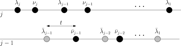
Figure 24. We expand sum with respect to the jump $t=c_{j-1}=\bar{\nu}_{j-1}-\bar{\lambda}_{j-1}$ of the leftmost particle on the $(j-1)$-st level. Note that the signatures $\nu,\lambda,\bar{\nu}$ are fixed, while the positions of particles $\bar{\lambda}_{i}$ vary in the sum.

The left-hand side of (2.25) divided by the right-hand side of the same equation is equal to

$$\sum_{\bar{\lambda}}\mathscr{V}_{j}(\lambda\to\nu\mid\bar{\lambda}\to\bar{\nu})\frac{\psi_{\lambda/\bar{\lambda}}\phi_{\bar{\nu}/\bar{\lambda}}}{\psi_{\nu/\bar{\nu}}\phi_{\nu/\lambda}}$$

$$=\sum_{t\in I}\sum_{\tilde{\lambda}\in J(t)}\underbrace{\binom{t}{\nu_{j}-\lambda_{j}}_{q^{-1}}\frac{(q^{\lambda_{j-1}-\bar{\nu}_{j-1}+t};q^{-1})_{\nu_{j}-\lambda_{j}}(q^{\tilde{\lambda}_{j-2}-\lambda_{j-1}};q^{-1})_{t-\nu_{j}+\lambda_{j}}}{(q^{\tilde{\lambda}_{j-2}-\bar{\nu}_{j-1}+t};q^{-1})_{t}}q^{(\lambda_{j-1}-\bar{\nu}_{j-1}+t)(t-\nu_{j}+\lambda_{j})}}_{\boldsymbol{\varphi}_{q^{-1},q^{\tilde{\lambda}_{j-2}-\lambda_{j-1}},q^{\tilde{\lambda}_{j-2}-\bar{\nu}_{j-1}+t}}(t-\nu_{j}+\lambda_{j}\mid t)}$$

$$\hskip 30.0pt\times\mathscr{V}_{j-1}(\lambda^{-}+[t-\nu_{j}+\lambda_{j}]_{\textnormal{lm}}\to\nu^{-}\mid\tilde{\lambda}\to\bar{\nu}^{-})\cdot\frac{\psi_{\lambda^{-}+[t-\nu_{j}+\lambda_{j}]_{\textnormal{lm}}/\tilde{\lambda}}\phi_{\bar{\nu}^{-}/\tilde{\lambda}}}{\psi_{\nu^{-}/\bar{\nu}^{-}}\phi_{\nu^{-}/\lambda^{-}+[t-\nu_{j}+\lambda_{j}]_{\textnormal{lm}}}}$$

$$\hskip 30.0pt\times\underbrace{\frac{\binom{\lambda_{j-1}-\lambda_{j}}{\bar{\nu}_{j-1}-t-\lambda_{j}}_{q}}{\binom{\nu_{j-1}-\nu_{j}}{\bar{\nu}_{j-1}-\nu_{j}}_{q}}\cdot\frac{\binom{\tilde{\lambda}_{j-2}-\bar{\nu}_{j-1}+t}{t}_{q}}{\binom{\lambda_{j-1}-\lambda_{j}}{\nu_{j}-\lambda_{j}}_{q}}\cdot\frac{(q^{\nu_{j-1}-\lambda_{j-1}};q^{-1})_{t-\nu_{j}+\lambda_{j}}}{(q^{\tilde{\lambda}_{j-2}-\lambda_{j-1}};q^{-1})_{t-\nu_{j}+\lambda_{j}}}}_{\frac{\psi_{\lambda/\bar{\lambda}}\psi_{\nu^{-}/\bar{\nu}^{-}}}{\psi_{\lambda^{-}+[t-\nu_{j}+\lambda_{j}]_{\textnormal{lm}}/\tilde{\lambda}}\psi_{\nu/\bar{\nu}}}\cdot\frac{\phi_{\bar{\nu}/\bar{\lambda}}\phi_{\nu^{-}/\lambda^{-}+[t-\nu_{j}+\lambda_{j}]_{\textnormal{lm}}}}{\phi_{\nu/\lambda}\phi_{\bar{\nu}^{-}/\tilde{\lambda}}}}$$

$$=\sum_{t\in I}\bigg{(}\boldsymbol{\varphi}_{q^{-1},q^{\nu_{j-1}-\bar{\nu}_{j-1}},q^{\nu_{j-1}-\nu_{j}}}(t-\nu_{j}+\lambda_{j}\mid\nu_{j-1}-\lambda_{j-1})$$

$$\hskip 30.0pt\times\sum_{\tilde{\lambda}\in J(t)}\mathscr{V}_{j-1}(\lambda^{-}+[t-\nu_{j}+\lambda_{j}]_{\textnormal{lm}}\to\nu^{-}\mid\tilde{\lambda}\to\bar{\nu}^{-})\cdot\frac{\psi_{\lambda^{-}+[t-\nu_{j}+\lambda_{j}]_{\textnormal{lm}}/\tilde{\lambda}}\phi_{\bar{\nu}^{-}/\tilde{\lambda}}}{\psi_{\nu^{-}/\bar{\nu}^{-}}\phi_{\nu^{-}/\lambda^{-}+[t-\nu_{j}+\lambda_{j}]_{\textnormal{lm}}}}\bigg{)}$$

$$=\sum_{t\in I}\boldsymbol{\varphi}_{q^{-1},q^{\nu_{j-1}-\bar{\nu}_{j-1}},q^{\nu_{j-1}-\nu_{j}}}(t-\nu_{j}+\lambda_{j}\mid\nu_{j-1}-\lambda_{j-1})=1.$$

Above $\mathscr{V}_{j-1}$ and $\mathscr{V}_{j}$ have the same value of the parameter $a=a_{j}$. We have also used the fact that

$$|\nu|-|\lambda|-|\bar{\nu}|+|\bar{\lambda}| =|\nu^{-}|-|\lambda^{-}|+\nu_{j}-\lambda_{j}-|\bar{\nu}^{-}|+|\bar{\lambda}^{-}|-\bar{\nu}_{j-1}+\bar{\lambda}_{j-1}$$

$$=|\nu^{-}|-|\lambda^{-}+[t-\nu_{j}+\lambda_{j}]_{\textnormal{lm}}|-|\bar{\nu}^{-}|+|\bar{\lambda}^{-}|,$$

hence $\mathscr{V}_{j}(\lambda\to\nu\mid\bar{\lambda}\to\bar{\nu})$ involves the same power of $\alpha a_{j}$ as $\mathscr{V}_{j-1}(\lambda^{-}+[t-\nu_{j}+\lambda_{j}]_{\textnormal{lm}}\to\nu^{-}\mid\bar{\lambda}^{-}\to\bar{\nu}^{-})$. Also, (6.10) implies that $\boldsymbol{\varphi}_{q^{-1},q^{\nu_{j-1}-\bar{\nu}_{j-1}},q^{\nu_{j-1}-\nu_{j}}}(t-\nu_{j}+\lambda_{j}\mid\nu_{j-1}-\lambda_{j-1})$ is nonzero only for $t\in I$, hence one gets $1$ after summing these quantities over $t\in I$.

This concludes the proof, and also establishes Theorem 1.3 from Introduction. ∎

6.3. Geometric $q$-PushTASEP

Under the dynamics $\mathscr{Q}^{q}_{\textnormal{row}}[\alpha]$ we have just constructed, the rightmost $N$ particles $\lambda^{(j)}_{1}$ of the interlacing array evolve in a marginally Markovian manner (i.e., their evolution does not depend on the dynamics of the rest of the interlacing array). Namely, at each discrete time step $t\to t+1$ the bottommost particle is updated as $\lambda^{(1)}_{1}(t+1)=\lambda^{(1)}_{1}(t)+V_{1}$, and for any $j=2,\ldots,N$ if we let $\mathsf{gap}_{j}(t)=\lambda^{(j)}_{1}(t)-\lambda^{(j-1)}_{1}(t)$ be the gap between the rightmost particles on the $(j-1)$-st and the $j$-th levels at time $t$, then

$$\lambda^{(j)}_{1}(t+1)=\lambda^{(j)}_{1}(t)+V_{j}+W_{j,t}$$

for an independent random variable $W_{j,t}$ distributed according to

$$\boldsymbol{\varphi}_{q^{-1},q^{\mathsf{gap}_{j}(t)},0}\big{(}\cdot\mid\lambda^{(j-1)}_{1}(t+1)-\lambda^{(j-1)}_{1}(t)\big{)}.$$

The random variable $V_{j}$ (recall that it has the $q$-geometric distribution with parameter $\alpha a_{j}$ which is resampled during each time step) represents an independent jump of $\lambda^{(j)}_{1}$. The variable $W_{j,t}$ represents the pushing of $\lambda^{(j)}_{1}$ by the move of $\lambda^{(j-1)}_{1}$.

This evolution of the rightmost particles $\lambda^{(j)}_{1}$, $1\leq j\leq N$, leads to a new interacting particle system on $\mathbb{Z}$ which we call the (discrete time) geometric $q$-PushTASEP.

6.4. Column insertion dynamics $\mathscr{Q}^{q}_{\textnormal{col}}[\alpha]$. Description and discussion

Let us now describe one time step $\boldsymbol{\lambda}\to\boldsymbol{\nu}$ of the multivariate Markov dynamics $\mathscr{Q}^{q}_{\textnormal{col}}[\alpha]$ on $q$-Whittaker processes of depth $N$. As in the previous case, the bottommost particle of the interlacing array is updated as $\nu_{1}^{(1)}=\lambda_{1}^{(1)}+X$ for a $q$-geometric random variable $X$ with parameter $\alpha a_{1}$. Next, sequentially for each $j=2,\ldots,N$, given the movement $\bar{\lambda}\to\bar{\nu}$ at level $j-1$, we will randomly update $\lambda\to\nu$ at level $j$. To describe this update we write, as usual,

$$\bar{\nu}-\bar{\lambda}=\sum_{i=1}^{j-1}c_{i}\bar{\mathrm{e}}_{i},\qquad c_{i}\in\mathbb{Z}_{\geq 0}.$$

All randomness during this update comes from a collection of $3j$ dependent random variables $X_{1},\ldots,X_{j},Y_{1},\ldots,Y_{j},Z_{1},\ldots,Z_{j}$ (they are resampled during each time step), and

$$\nu_{j-i+1}-\lambda_{j-i+1}=\underbrace{X_{i}}_{\text{voluntary jump}}+\underbrace{Y_{i}}_{\text{push from $\bar{\lambda}_{j-i+1}$}}+\underbrace{Z_{i}}_{\text{push from the ``stabilization fund''}},\qquad i=1,\ldots,j.$$

(It will be convenient to let $i$ represent the position of the particle counted from the left.) Observe that $Y_{1}$ must be identically zero. The “stabilization fund” means the leftover push from the first $i-2$ particles from the left at level $j-1$ (i.e., from $\bar{\lambda}_{j-1},\ldots,\bar{\lambda}_{j-i+2}$) (in particular, $Z_{1}$ and $Z_{2}$ are identically zero).

Let us first formally define the distribution of all the parts of the jumps:

1. Set $\theta_{1}:=1$. For $i$ from $1$ to $j$ sample $X_{i}$ according to

   $$X_{i}\sim\boldsymbol{\varphi}_{q,\alpha a_{j}\theta_{i},0}(\cdot\mid\bar{\lambda}_{j-i}-\lambda_{j-i+1})$$ (6.12)

   and set

   $$\theta_{i+1}:=\theta_{i}q^{\bar{\lambda}_{j-i}-\lambda_{j-i+1}-X_{i}}.$$

   The jump $X_{i}$ comes from the input $V_{j}$, see Remark 6.7 below. Here the convention $\bar{\lambda}_{0}=+\infty$ applies when $i=j$.

2. Set $Y_{1}:=0$. For $i$ from $2$ to $j-1$ take $Y_{i}=y$ with probability

   $$Y_{i}\sim\boldsymbol{\varphi}_{q^{-1},q^{c_{j-i+1}},q^{\bar{\lambda}_{j-i}-\bar{\lambda}_{j-i+1}}}(\bar{\lambda}_{j-i}-\lambda_{j-i+1}-X_{i}-y\mid\bar{\lambda}_{j-i}-\lambda_{j-i+1}-X_{i}).$$ (6.13)

   Finally, set $Y_{j}:=c_{1}$.

3. Set $r_{1}=r_{2}=1$ and $Z_{1}=Z_{2}:=0$. Set $r_{3}:=r_{2}q^{c_{j-1}-Y_{2}}$. For $i$ from $3$ to $j-1$ take $Z_{i}=z$ with probability

   $$Z_{i}\sim\boldsymbol{\varphi}_{q^{-1},r_{i},0}(\bar{\lambda}_{j-i}-\lambda_{j-i+1}-X_{i}-Y_{i}-z\mid\bar{\lambda}_{j-i}-\lambda_{j-i+1}-X_{i}-Y_{i})$$ (6.14)

   and set

   $$r_{i+1}:=r_{i}q^{c_{j-i+1}-Y_{i}-Z_{i}}.$$

   Finally, let $Z_{j}:=\log_{q}r_{j}$.

Remark 6.5.

For fixed $s,u,d\geq 0$ (possibly $u=\infty$) and $D\to\infty$ observe that

$$\boldsymbol{\varphi}_{q^{-1},q^{s},q^{u+D}}(D-d\mid D)=q^{(s-d)(D-d)}(q^{s};q^{-1})_{d}\binom{D}{d}_{q}\frac{(q^{u+D-s};q^{-1})_{D-d}}{(q^{u+D};q^{-1})_{D}}\to\textbf{1}_{d=s}.$$

Therefore, the definitions of $Z_{j}=\log_{q}r_{j}$ and $Y_{j}=c_{1}$ are consistent with the definitions of $Z_{i}$ and $Y_{i}$ ($i<j$), respectively. In words, the consistency for $Z_{j}$ means that the stabilization fund is depleted for the push of the rightmost particle on the $j$-th level. The consistency for $Y_{j}$ means that the whole value of the jump of the rightmost particle on the $(j-1)$-st level is transferred to the rightmost particle on the $j$-th level via immediate pushing.

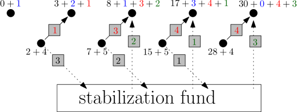
Figure 25. An example of a step of $\mathscr{Q}^{q}_{\textnormal{col}}[\alpha]$ at levels 4 and 5.

Lemma 6.6.

If $\bar{\lambda}\prec_{\mathsf{h}}\bar{\nu}$, $\bar{\lambda}\prec_{\mathsf{h}}\lambda$ and $\mathscr{U}_{j}(\lambda\to\nu\mid\bar{\lambda}\to\bar{\nu})>0$, then $\bar{\nu}\prec_{\mathsf{h}}\nu$ and $\lambda\prec_{\mathsf{h}}\nu$.

Proof.

It is straightforward from the definition of the dynamics $\mathscr{Q}^{q}_{\textnormal{col}}[\alpha]$ that $\nu_{j-i+1}\leq\bar{\lambda}_{j-i}\leq\min(\bar{\nu}_{j-i},\lambda_{j-i})$. Also for $2\leq i\leq j$ (6.13) together with (6.10) implies that $\bar{\lambda}_{j-i}-\lambda_{j-i+1}-X_{i}-Y_{i}\leq\bar{\lambda}_{j-i}-\bar{\lambda}_{j-i+1}-c_{j-i+1}$, hence $\nu_{j-i+1}\geq\lambda_{j-i+1}+X_{i}+Y_{i}\geq\bar{\nu}_{j-i+1}$. It follows that the interlacing properties are preserved. ∎

In the rest of this subsection we will describe the column insertion dynamics in words, and also discuss its various properties. The (rather involved) proof that this dynamics acts on $q$-Whittaker processes in a desired way is postponed to the next subsection.

There are two stages of the update of particle positions $\lambda_{j},\lambda_{j-1},\ldots,\lambda_{1}$, performed in order from left to right, which we will describe below.

During the first stage of the update, the particles at level $j$ level make voluntary jumps in order from left to right. The value $X_{i}$ of the voluntary jump of $\lambda_{j+1-i}$ depends on the previous jump $X_{i-1}$, where $2\leq i\leq j$. Indeed, this dependence comes from the parameters $\theta_{i}$ (note that they are nonincreasing in $i$), see (6.12). Note that unlike the $\mathscr{Q}^{q}_{\textnormal{row}}[\alpha]$ case, in which all random movements not coming from pushing are restricted to the right edge, in the case of $\mathscr{Q}^{q}_{\textnormal{col}}[\alpha]$ any particle might make a voluntary jump.

Remark 6.7.

The random variable $X_{1}+\ldots+X_{j}$ has the $q$-geometric distribution with parameter $\alpha a_{j}$, as it should be by Remark 2.10 and the discussion of §3.2. This is seen by applying inductively the next Lemma.

Lemma 6.8.

Let $A$ and $B$ be random variables such that $A$ is distributed according to $\boldsymbol{\varphi}_{q,\alpha,0}(\cdot\mid a)$, and $B$ given $A$ is distributed according to $\boldsymbol{\varphi}_{q,\alpha q^{a-A},0}(\cdot\mid b)$ (where $b$ might be $+\infty$). Then $A+B$ is distributed according to $\boldsymbol{\varphi}_{q,\alpha,0}(\cdot\mid a+b)$.

Proof.

Indeed, we have

$$Prob(A+B=y)=\sum_{s=0}^{y}Prob(A=s)Prob(B=y-s|A=s)$$

$$\hskip 30.0pt=\sum_{s=0}^{y}\alpha^{s}(\alpha;q)_{a-s}\binom{a}{s}_{q}(\alpha q^{a-s})^{y-s}(\alpha q^{a-s};q)_{b-y+s}\binom{b}{y-s}_{q}$$

$$\hskip 30.0pt=\sum_{s=0}^{y}\alpha^{y}(\alpha;q)_{a+b-y}q^{a(y-s)}\frac{(q^{a};q^{-1})_{s}(q^{b};q^{-1})_{y-s}}{(q;q)_{y}}q^{-s(y-s)}\binom{y}{s}_{q}$$

$$\hskip 30.0pt=\alpha^{y}(\alpha;q)_{a+b-y}\binom{a+b}{y}_{q}\cdot\sum_{s=0}^{y}\boldsymbol{\varphi}_{q^{-1},q^{a},q^{a+b}}(y-s\mid y)$$

$$\hskip 30.0pt=\boldsymbol{\varphi}_{q,\alpha,0}(y\mid a+b),$$

which establishes the desired statement. ∎

The second stage of the update consists of pushing, in order from left to right. We start an initially empty stabilization fund, which will collect impulses not immediately used for pushing, and will be a source of the pushes $Z_{i}$. The value of the stabilization fund just before the movement of $\lambda_{j+1-i}$ is $\log_{q}r_{i}$ (by agreement, $r_{1}=r_{2}=1$ always). For each $i$ ranging from $2$ to $j$, the following three steps happen:

(6.15)

One can also think that the above two update stages are performed together for each particle $\lambda_{j},\lambda_{j-1},\ldots,\lambda_{1}$.

Proposition 6.9.

One can switch the order of the lower left neighbor pushing and stabilization fund pushing (i.e., steps (1) and (2) in (6.15)) without changing the dynamics.

Proof.

Fix $k=2,\ldots,j$. Suppose that after the voluntary displacement stage the distance from the $k$-th particle from the left at level $j$ (denote this particle by $P$) to $\bar{\lambda}_{j+1-k}$ is $h:=\bar{\lambda}_{j-k}-\lambda_{j-k+1}-X_{j-k+1}$. Also set $\ell:=\bar{\nu}_{j-k+1}-\bar{\lambda}_{j-k+1}$, $b:=\bar{\lambda}_{j-k}-\bar{\lambda}_{j-k+1}$, and let the current size of the stabilization fund be $R$.

If the steps (1) and (2) in (6.15) are not interchanged, then the probability that $P$ jumps by $s\geq 0$ is

$$\sum_{y=0}^{s}\boldsymbol{\varphi}_{q^{-1},q^{\ell},q^{b}}(h-y\mid h)\boldsymbol{\varphi}_{q^{-1},q^{R},0}(h-s\mid h-y).$$

If the steps (1) and (2) in (6.15) are interchanged, then the same probability is given by

$$\sum_{y=0}^{s}\boldsymbol{\varphi}_{q^{-1},q^{R},0}(h-s+y\mid h)\boldsymbol{\varphi}_{q^{-1},q^{\ell},q^{b}}(h-s\mid h-s+y).$$

After dividing each of these two expressions by $\frac{q^{(R+\ell)(h-s)}(q^{b-\ell};q^{-1})_{h-s}}{(q^{b};q^{-1})_{h-s}}\binom{h}{s}_{q^{-1}}$ we arrive to the following identity we need to verify:

$$\sum_{y=0}^{s}\binom{s}{y}_{q^{-1}}q^{\ell(s-y)}(q^{\ell};q^{-1})_{y}(q^{R};q^{-1})_{s-y}(q^{b-\ell-h+s};q^{-1})_{s-y}\\ =\sum_{y=0}^{s}\binom{s}{y}_{q^{-1}}q^{Ry}(q^{\ell};q^{-1})_{y}(q^{R};q^{-1})_{s-y}(q^{b-h+1};q)_{s-y}.$$ (6.16)

We are very grateful to Christian Krattenthaler for providing us with a proof of the $q$-binomial identity (6.16), which we reproduce below.

First, use a transformation formula for ${}_{3}\phi_{2}$ series [36, (III.12)]:

$${}_{3}\phi_{2}\left[\begin{array}[]{c}q^{-n},b,c\\ d,e\end{array};q,q\right]=\frac{(e/c;q)_{n}}{(e;q)_{n}}c^{n}{{}_{3}\phi_{2}}\left[\begin{array}[]{c}q^{-n},c,d/b\\ d,cq^{1-n}/e\end{array};q,\frac{bq}{e}\right]$$

Sending $b\to 0$ we obtain

$$_{3}\phi_{2}\left[\begin{array}[]{c}q^{-n},0,c\\ d,e\end{array};q,q\right]=\frac{(e/c;q)_{n}}{(e;q)_{n}}c^{n}{{}_{2}\phi_{2}}\left[\begin{array}[]{c}q^{-n},c\\ d,cq^{1-n}/e\end{array};q,\frac{dq}{e}\right]$$ (6.21)

Multiply both sides of (6.21) by $c^{-n}(d;q)_{n}(e;q)_{n}$ to obtain

$$c^{-n}\sum_{y=0}^{n}\frac{(q^{-n};q)_{y}}{(q;q)_{y}}(c;q)_{y}(dq^{n-1};q^{-1})_{n-y}(eq^{n-1};q^{-1})_{n-y}q^{y}=$$

$$\sum_{y=0}^{n}\frac{(q^{-n};q)_{y}(e/c;q)_{n}}{(q;q)_{y}(cq^{1-n}/e;q)_{y}}(c;q)_{y}(dq^{n-1};q^{-1})_{n-y}(-1)^{y}q^{y(y-1)/2}(dq/e)^{y}.$$

This equality can be rewritten as

$$\sum_{y=0}^{n}\binom{n}{y}_{q^{-1}}c^{y-n}(c^{-1};q^{-1})_{y}(dq^{n-1};q^{-1})_{n-y}(eq^{n-1};q^{-1})_{n-y}=$$

$$\sum_{y=0}^{n}\binom{n}{y}_{q^{-1}}(e/c;q)_{n-y}(c^{-1};q^{-1})_{y}(dq^{n-1};q^{-1})_{n-y}(dq^{n-1})^{y}.$$

Now make the substitution $n:=s$, $d:=q^{1+R-s}$, $c:=q^{-\ell}$, $e:=q^{1+b-h-\ell}$ to arrive to (6.16). ∎

Remark 6.10.

(Schur degeneration) If one sets $q=0$, then the dynamics $\mathscr{Q}^{q}_{\textnormal{col}}[\alpha]$ reduces to the dynamics $\mathscr{Q}^{q=0}_{\textnormal{col}}[\alpha]$ on Schur processes based on the classical Robinson–Schensted–Knuth column insertion (§4.3). Indeed, observe that

$$\lim_{q\to 0}\boldsymbol{\varphi}_{q,uq^{t},0}(s\mid g)=\mathbf{1}_{s=0}\quad\text{for}\ t>0,\ \text{and}\quad\lim_{q\to 0}\boldsymbol{\varphi}_{q,u,0}(s\mid g)=(1-u+u\mathbf{1}_{s=g})u^{s}.$$

Thus, the first update stage (voluntary movements) reduces to the propagation of the impulse the leftmost particle receives (which has geometric distribution with parameter $\alpha a_{j}$). The lower left neighbor pushing due to (6.8) and the stabilization fund pushing together degenerate to performing $c_{j-1}+\cdots+c_{1}$ operations $\mathsf{push}$ (Definition 4.3) in order from left to right.

6.5. Column insertion dynamics $\mathscr{Q}^{q}_{\textnormal{col}}[\alpha]$. Proof

Theorem 6.11.

The dynamics $\mathscr{Q}^{q}_{\textnormal{col}}[\alpha]$ defined above satisfies the main equations (2.25), and hence preserves the class of $q$-Whittaker processes and adds a new usual parameter $\alpha$ to the specialization $\mathbf{A}$ as in (2.17).

Proof.

We aim to prove the desired statement by induction on $j$. To apply this induction, we will need a more general statement. To describe it, introduce the following notation. For a nonnegative integer $h$, use $\mathscr{U}_{j}^{h}(\lambda\to\nu\mid\bar{\lambda}\to\bar{\nu})$ to denote the probability that transition $\bar{\lambda}\to\bar{\nu}$ on the $(j-1)$-st level spurs a transition $\lambda\to\nu$ on the $j$-th level according to the rules of $\mathscr{Q}^{q}_{\textnormal{col}}[\alpha]$ specified above, but modified so that $Z_{2}=z$ with probability

$$\boldsymbol{\varphi}_{q^{-1},r_{2},0}(\bar{\lambda}_{j-2}-\lambda_{j-1}-X_{2}-Y_{2}-z\mid\bar{\lambda}_{j-2}-\lambda_{j-1}-X_{2}-Y_{2}),\qquad r_{2}:=q^{h}.$$

Note that the original dynamics $\mathscr{Q}^{q}_{\textnormal{col}}[\alpha]$ has $r_{2}=1$. In other words, the modification $\mathscr{U}_{j}^{h}$ means that we introduce an additional impulse of size $h$ which is distributed among particles at level $j$ (except for $\lambda_{j}$), as if coming from (nonexistent) particles preceding the leftmost particle on the $(j-1)$-st level.

Let $\sigma:=|\nu^{-}|-|\lambda^{-}|-|\bar{\nu}|+|\bar{\lambda}|$ (recall that the notation $\mu^{-}$ means $\mu$ without the last coordinate). Under the modified probabilities $\mathscr{U}_{j}^{h}$ as above, $\sigma-h$ is a sum of voluntary movements of particles on the $j$-th level except for the leftmost one. Note also that $\mathscr{U}_{j}^{h}(\lambda\to\nu\mid\bar{\lambda}\to\bar{\nu})=0$ for $h>\sigma$.

For the purposes of the proof, let (see Fig. 26)

$$a:=\lambda_{j},\qquad k:=\nu_{j}-\lambda_{j},\qquad b:=\bar{\nu}_{j-1},\qquad t:=\bar{\nu}_{j-1}-\bar{\lambda}_{j-1},$$

$$c:=\lambda_{j-1},\qquad d:=\bar{\nu}_{j-2},\qquad s:=\bar{\nu}_{j-2}-\bar{\lambda}_{j-2},$$

$$\ell:=\nu_{j-1}-\lambda_{j-1},\qquad x:=X_{2}\qquad y:=Y_{2}.$$

For a nonnegative integer $H$ define

$$\tilde{\mathscr{U}}_{j}^{H}(\lambda\to\nu\mid\bar{\lambda}\to\bar{\nu}):=\sum_{h=0}^{H}\binom{H}{h}_{q^{-1}}q^{(H-h)\sigma+h(b-t-a-k)}\mathscr{U}_{j}^{h}(\lambda\to\nu\mid\bar{\lambda}\to\bar{\nu}).$$ (6.22)

In particular, $\tilde{\mathscr{U}}_{j}^{0}(\lambda\to\nu\mid\bar{\lambda}\to\bar{\nu})=\mathscr{U}_{j}(\lambda\to\nu\mid\bar{\lambda}\to\bar{\nu})$. In general, the quantities $\tilde{\mathscr{U}}_{j}^{H}$ are not probability distributions in $\nu$. Their only meaning is that they come up in the inductive proof below.

With all the above notation we are now able to describe and prove the generalized statement which we will prove by induction:

$$\sum_{\bar{\lambda}\in\mathbb{GT}^{+}_{j-1}}\tilde{\mathscr{V}}_{j}^{H}(\lambda\to\nu\mid\bar{\lambda}\to\bar{\nu})\frac{\psi_{\lambda/\bar{\lambda}}\phi_{\bar{\nu}/\bar{\lambda}}}{\psi_{\nu/\bar{\nu}}\phi_{\nu/\lambda}}=1\qquad\text{for any $H\geq 0$.}$$ (6.23)

Here and below $\tilde{\mathscr{V}}_{j}^{H}$ is related to $\tilde{\mathscr{U}}_{j}^{H}$ as in (6.11). For $H=0$ this statement gives us (2.25).

For $j=1$ we have $\sigma=0$, so only the term $h=0$ contributes to (6.22). Therefore, checking this induction base is the same as in the proof for $\mathscr{Q}^{q}_{\textnormal{row}}[\alpha]$ dynamics.

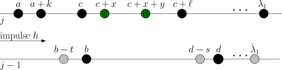
Figure 26. We expand sum with respect to jump $t=c_{j-1}=\bar{\nu}_{j-1}-\bar{\lambda}_{j-1}$ of the leftmost particle on the $(j-1)$-st level, voluntary movement $x$ of the second leftmost particle on the $j$-th level and push $y$ from the leftmost particle on the $(j-1)$-st level.

Let us now perform the inductive step. Denote by $I$ the range of $(t,x,y,h)$, such that

$$t,x,y,h\geq 0,\qquad x+y\leq\ell,\qquad h+t+x-\ell\geq 0,\qquad t\leq b-a-k.$$

Then we may write (see Fig. 26)

$$\sum_{\bar{\lambda}\in\mathbb{GT}^{+}_{j-1}}\tilde{\mathscr{V}}_{j}^{H}(\lambda\to\nu\mid\bar{\lambda}\to\bar{\nu})\frac{\psi_{\lambda/\bar{\lambda}}\phi_{\bar{\nu}/\bar{\lambda}}}{\psi_{\nu/\bar{\nu}}\phi_{\nu/\lambda}}{}$$

$$\hskip 20.0pt=\sum_{(t,x,y,h)\in I}\frac{(q;q)_{H}}{(q;q)_{h}(q;q)_{H-h}}\frac{(q;q)_{c-a}}{(q;q)_{b-t-a}(q;q)_{c-b+t}}\frac{(q;q)_{b-a-k}(q;q)_{c+\ell-b}}{(q;q)_{c+\ell-a-k}}\frac{(q;q)_{d-s-b+t}}{(q;q)_{t}(q;q)_{d-s-b}}$$

$$\hskip 40.0pt\times\frac{(q;q)_{k}(q;q)_{c-a-k}}{(q;q)_{c-a}}\frac{(q;q)_{b-t-a}}{(q;q)_{k}(q;q)_{b-t-a-k}}\frac{(q;q)_{d-s-c}}{(q;q)_{x}(q;q)_{d-s-c-x}}\frac{(q;q)_{d-s-c-x}}{(q;q)_{y}(q;q)_{d-s-c-x-y}}$$

$$\hskip 40.0pt\times\frac{(q^{t};q^{-1})_{y}(q^{d-s-b};q^{-1})_{d-s-c-x-y}}{(q^{d-s-b+t};q^{-1})_{d-s-c-x}}\frac{(q;q)_{d-s-c-x-y}}{(q;q)_{\ell-x-y}(q;q)_{d-s-c-\ell}}(q^{h};q^{-1})_{\ell-x-y}$$

$$\hskip 40.0pt\times q^{-h(H-h)-y(d-s-c-x-y)-(d-s-c-\ell)(\ell-x-y)+t(d-s-c-x-y)}$$

$$\hskip 40.0pt\times q^{h(d-s-c-\ell)+(H-h)\sigma+h(b-t-a-k)+(b-t-a-k)x+(b-t-a-k+\ell-x)(\sigma-x-h)}$$

$$\hskip 60.0pt\times\sum_{\tilde{\lambda}\in\mathbb{GT}^{+}_{j-2}}\mathscr{V}_{j}^{h+t+x-\ell}(\lambda^{-}\to\nu^{-}\mid\tilde{\lambda}\to\bar{\nu}^{-})\frac{\psi_{\lambda^{-}/\tilde{\lambda}}\phi_{\bar{\nu}^{-}/\tilde{\lambda}}}{\psi_{\nu^{-}/\bar{\nu}^{-}}\phi_{\nu^{-}/\lambda^{-}}}$$

$$\hskip 20.0pt=\sum_{r=0}^{H+B}\binom{H+B}{r}_{q^{-1}}q^{(H+B-r)(\sigma-\ell+t)+r(d-s-c-\ell)}$$

$$\hskip 60.0pt\times\sum_{\tilde{\lambda}\in\mathbb{GT}^{+}_{j-2}}\mathscr{V}_{j}^{r}(\lambda^{-}\to\nu^{-}\mid\tilde{\lambda}\to\bar{\nu}^{-})\frac{\psi_{\lambda^{-}/\tilde{\lambda}}\phi_{\bar{\nu}^{-}/\tilde{\lambda}}}{\psi_{\nu^{-}/\bar{\nu}^{-}}\phi_{\nu^{-}/\lambda^{-}}}$$

$$\hskip 20.0pt=\sum_{\tilde{\lambda}\in\mathbb{GT}^{+}_{j-2}}\tilde{\mathscr{V}}_{j}^{H+B}(\lambda^{-}\to\nu^{-}\mid\tilde{\lambda}\to\bar{\nu}^{-})\frac{\psi_{\lambda^{-}/\tilde{\lambda}}\phi_{\bar{\nu}^{-}/\tilde{\lambda}}}{\psi_{\nu^{-}/\bar{\nu}^{-}}\phi_{\nu^{-}/\lambda^{-}}}$$

$$\hskip 20.0pt=1.$$

Here we have applied Proposition 6.12 (see below) with $A=H$, $B=b-a-k$, $C=c-b+\ell$, where $r:=h+t-\ell+x$ is the value of the stabilization fund just before the push of the third leftmost particle on the $j$-th level plus the value of the additional impulse in the inductive assumption. This completes the inductive step in proving (6.23), and thus implies the theorem. ∎

Proposition 6.12.

For $A,B,C,\ell,r\geq 0$, such that $A+B\geq r$ and $B+C\geq\ell$, one has

$$\sum_{t=0}^{B}\sum_{x=0}^{\ell}\sum_{y=0}^{\ell-x}\Bigg{[}\binom{\ell}{x,\ y}_{q^{-1}}\binom{B}{t}_{q^{-1}}(q^{t};q^{-1})_{y}(q^{r+\ell-x};q^{-1})_{t}(q^{r+\ell-t-x};q^{-1})_{\ell-x-y}\frac{(q;q)_{r}}{(q;q)_{r+\ell-x}}\\ \times\frac{(q;q)_{A}}{(q;q)_{A+B}}\frac{(q^{A+B-r};q^{-1})_{B-t+\ell-x}(q^{C+t};q^{-1})_{\ell}(q^{C};q^{-1})_{\ell-x-y}}{(q^{B+C};q^{-1})_{\ell}(q^{C+t};q^{-1})_{\ell-x}}\\ \times q^{t(\ell-x-y)+(r+\ell-x)(B-t)+(A+B-r)x}\Bigg{]}=1.$$

Here and thereafter we use $q$-multinomial notation $\displaystyle\binom{n}{m,\ k}_{q}:=\frac{(q;q)_{n}}{(q;q)_{k}(q;q)_{m}(q;q)_{n-m-k}}$.

We are extremely grateful to Christian Krattenthaler for providing us with a proof of this proposition. We reproduce the proof below.

Proof.

The left hand side of the equality can be expressed as a power series in $q^{A},q^{r},q^{C}$, hence we can set $\alpha=q^{A}$, $\beta=q^{r}$, $\gamma=q^{C}$ and prove a more general equality:

$$\sum_{t=0}^{B}\sum_{x=0}^{\ell}\sum_{y=0}^{\ell-x}\Bigg{[}\binom{\ell}{x,\ y}_{q^{-1}}\binom{B}{t}_{q^{-1}}(q^{t};q^{-1})_{y}\frac{(\beta q^{\ell-x};q^{-1})_{t+\ell-x-y}}{(\beta q^{\ell-x};q^{-1})_{\ell-x}}\\ \times\frac{(\alpha q^{B}/\beta;q^{-1})_{B-t+\ell-x}(\gamma q^{t};q^{-1})_{\ell}(\gamma;q^{-1})_{\ell-x-y}}{(\alpha q^{B};q^{-1})_{B}(\gamma q^{B};q^{-1})_{\ell}(\gamma q^{t};q^{-1})_{\ell-x}}\times\alpha^{x}\beta^{B-t-x}q^{-ty+B\ell}\Bigg{]}=1.$$

By first summing over $y$, the left hand side can be written as

$$\sum_{t=0}^{B}\sum_{x=0}^{\ell}\Bigg{[}{{}_{3}\phi_{2}}\left[\begin{array}[]{c}q^{-t},0,q^{-\ell+x}\\ \beta q^{1-t},\gamma q^{1-\ell+x}\end{array};q,q\right]\binom{\ell}{x}_{q^{-1}}\binom{B}{t}_{q^{-1}}\frac{(\beta q^{\ell-x};q^{-1})_{t+\ell-x}}{(\beta q^{\ell-x};q^{-1})_{\ell-x}}\\ \times\frac{(\alpha q^{B}/\beta;q^{-1})_{B-t+\ell-x}(\gamma q^{t};q^{-1})_{\ell}(\gamma;q^{-1})_{\ell-x}}{(\alpha q^{B};q^{-1})_{B}(\gamma q^{B};q^{-1})_{\ell}(\gamma q^{t};q^{-1})_{\ell-x}}\times\alpha^{x}\beta^{B-t-x}q^{B\ell}\Bigg{]}.$$

We now apply transformation formula (6.21) to rewrite this as

$$=\sum_{t=0}^{B}\sum_{x=0}^{\ell}\Bigg{[}{{}_{2}\phi_{2}}\left[\begin{array}[]{c}q^{-t},q^{-\ell+x}\\ \beta q^{1-t},q^{-t}/\gamma\end{array};q,\beta q^{1+\ell-t-x}/\gamma\right]\binom{\ell}{x}_{q^{-1}}\binom{B}{t}_{q^{-1}}\frac{(\beta q^{\ell-x};q^{-1})_{t+\ell-x}}{(\beta q^{\ell-x};q^{-1})_{\ell-x}}\frac{(\gamma q;q)_{t}}{(\gamma q^{1-\ell+x};q)_{t}}$$

$$\hskip 40.0pt\times\frac{(\alpha q^{B}/\beta;q^{-1})_{B-t+\ell-x}(\gamma q^{t};q^{-1})_{\ell}(\gamma;q^{-1})_{\ell-x}}{(\alpha q^{B};q^{-1})_{B}(\gamma q^{B};q^{-1})_{\ell}(\gamma q^{t};q^{-1})_{\ell-x}}\times\alpha^{x}\beta^{B-t-x}q^{B\ell-\ell t+tx}\Bigg{]}$$

$$\hskip 20.0pt=\sum_{t=0}^{B}\sum_{x=0}^{\ell}\sum_{y=0}^{\min\{t,\ell-x\}}\Bigg{[}(-1)^{y}\frac{(q^{-t};q)_{y}(q^{-\ell+x};q)_{y}}{(q^{-t}/\gamma;q)_{y}(\beta q^{1-t};q)_{y}(q;q)_{y}}\binom{\ell}{x}_{q^{-1}}\binom{B}{t}_{q^{-1}}\frac{(\gamma q;q)_{t}}{(\gamma q^{1-\ell+x};q)_{t}}$$

$$\hskip 40.0pt\times\frac{(\beta;q^{-1})_{t}(\alpha q^{B}/\beta;q^{-1})_{B-t+\ell-x}(\gamma q^{t};q^{-1})_{\ell}(\gamma;q^{-1})_{\ell-x}}{(\alpha q^{B};q^{-1})_{B}(\gamma q^{B};q^{-1})_{\ell}(\gamma q^{t};q^{-1})_{\ell-x}}$$

$$\hskip 40.0pt\times\alpha^{x}\beta^{B-t-x+y}\gamma^{-y}q^{B\ell+\ell y-\ell t+tx+y^{2}/2+y/2-ty-xy}\Bigg{]}$$

$$\hskip 20.0pt=\sum_{t=0}^{B}\sum_{y=0}^{\ell}\Bigg{[}{{}_{1}\phi_{1}}\left[\begin{array}[]{c}q^{-\ell+y}\\ \alpha q^{1-\ell+t}/\beta\end{array};q,\alpha q^{1+t-y}/\beta\right](-1)^{y}\frac{(q^{-\ell};q)_{y}(q^{-t};q)_{y}}{(q^{-t}/\gamma;q)_{y}(\beta q^{1-t};q)_{y}(q;q)_{y}}$$

$$\hskip 40.0pt\times\binom{B}{t}_{q^{-1}}\frac{(\beta;q^{-1})_{t}(\alpha q^{B}/\beta;q^{-1})_{B-t+\ell}(\gamma q^{t};q^{-1})_{\ell}}{(\alpha q^{B};q^{-1})_{B}(\gamma q^{B};q^{-1})_{\ell}}\times\beta^{B-t+y}\gamma^{-y}q^{B\ell-\ell t+\ell y+y^{2}/2+y/2-ty}\Bigg{]}.$$

The last equality is obtained by summing over $x$. We now use the summation formula [36, (II.5)]:

$${{}_{1}\phi_{1}}\left[\begin{array}[]{c}a\\ c\end{array};q,c/a\right]=\frac{(c/a;q)_{\infty}}{(c;q)_{\infty}},$$

and by summing over $y$ rewrite our expression as

$$=\sum_{t=0}^{B}\Bigg{[}{{}_{3}\phi_{2}}\left[\begin{array}[]{c}q^{-\ell},\beta q^{-t}/\alpha,q^{-t}\\ \beta q^{1-t},q^{-t}/\gamma\end{array};q,\alpha q^{1+\ell}/\gamma\right]\\ \times\binom{B}{t}_{q^{-1}}\frac{(\beta;q^{-1})_{t}(\alpha q^{B}/\beta;q^{-1})_{B-t+\ell}(\gamma q^{t};q^{-1})_{\ell}}{(\alpha q^{t}/\beta;q^{-1})_{\ell}(\alpha q^{B};q^{-1})_{B}(\gamma q^{B};q^{-1})_{\ell}}\times\beta^{B-t}q^{B\ell-\ell t}\Bigg{]}.$$

We now aim to use the transformation formula [36, (III.13)]:

$${{}_{3}\phi_{2}}\left[\begin{array}[]{c}q^{-n},b,c\\ d,e\end{array};q,deq^{n}/bc\right]=\frac{(e/c;q)_{n}}{(e;q)_{n}}{{}_{3}\phi_{2}}\left[\begin{array}[]{c}q^{-n},c,d/b\\ d,cq^{1-n}/e\end{array};q,q\right].$$ (6.28)

Applying it, we can rewrite our expression as

$$=\sum_{t=0}^{B}\Bigg{[}{{}_{3}\phi_{2}}\left[\begin{array}[]{c}q^{-\ell},q^{-t},\alpha q\\ \beta q^{1-t},\gamma q^{1-\ell}\end{array};q,q\right]$$

$$\hskip 40.0pt\times\binom{B}{t}_{q^{-1}}\frac{(1/\gamma;q)_{\ell}(\beta;q^{-1})_{t}(\alpha q^{B}/\beta;q^{-1})_{B-t+\ell}(\gamma q^{t};q^{-1})_{\ell}}{(\alpha q^{t}/\beta;q^{-1})_{\ell}(\alpha q^{B};q^{-1})_{B}(\gamma q^{B};q^{-1})_{\ell}(q^{-t}/\gamma;q)_{\ell}(q;q)_{y}}\times\beta^{B-t}q^{B\ell-\ell t}\Bigg{]}$$

$$\hskip 5.0pt=\sum_{t=0}^{B}\sum_{y=0}^{\ell}\Bigg{[}\binom{B}{t}_{q^{-1}}\frac{(q^{-\ell};q)_{y}(q^{-t};q)_{y}(\alpha q;q)_{y}(\gamma;q^{-1})_{\ell-y}(\beta q^{y};q^{-1})_{t}(\alpha q^{B}/\beta;q^{-1})_{B-t+\ell}}{(\alpha q^{t}/\beta;q^{-1})_{\ell}(\alpha q^{B};q^{-1})_{B}(\gamma q^{B};q^{-1})_{\ell}(\beta q^{y};q^{-1})_{y}(q;q)_{y}}\times\beta^{B-t}q^{B\ell+y}\Bigg{]}$$

$$\hskip 5.0pt=\sum_{y=0}^{\ell}\sum_{t=y}^{B}\Bigg{[}\binom{B-y}{t-y}_{q^{-1}}\frac{\beta^{B-t}(\beta;q^{-1})_{t-y}(\alpha q^{B}/\beta;q^{-1})_{B-t}}{(\alpha q^{B};q^{-1})_{B-y}}\times\binom{\ell}{y}_{q^{-1}}\frac{q^{B(\ell-y)}(\gamma;q^{-1})_{\ell-y}(q^{B};q^{-1})_{y}}{(\gamma q^{B};q^{-1})_{\ell}}\Bigg{]}.$$

The fact that this expression is equal to $1$ now follows by applying (6.3) twice. ∎

6.6. Geometric $q$-TASEP

Under the dynamics $\mathscr{Q}^{q}_{\textnormal{col}}[\alpha]$, the leftmost $N$ particles $\lambda^{(j)}_{j}$ of the interlacing array evolve in a marginally Markovian manner.

Namely, let $\mathsf{gap}_{j}(t):=\lambda^{(j-1)}_{j-1}(t)-\lambda^{(j)}_{j}(t)$ be the gap between the consecutive leftmost particles at time $t$. We assume $\mathsf{gap}_{1}(t)=+\infty$. Then at each discrete time step $t\to t+1$ the leftmost particle on the $j$-th level is updated as

$$\lambda^{(j)}_{1}(t+1)=\lambda^{(j)}_{1}(t)+W_{j,t}$$

for an independent random variable $W_{j,t}$ distributed according to $\boldsymbol{\varphi}_{q,\alpha a_{j},0}(\cdot\mid\mathsf{gap}_{j}(t))$.

This evolution of $\lambda^{(j)}_{j}$, $1\leq j\leq N$, is the (discrete time) geometric $q$-TASEP which was introduced and studied in [8].

6.7. Small $\alpha$ continuous time limit

Let us send the parameter $\alpha$ to zero and simultaneously rescale time from discrete to continuous. Namely, set $\alpha:=(1-q)\Delta$, and let each discrete time step correspond to continuous time $\Delta$. In the limit $\Delta\to 0$, both dynamics $\mathscr{Q}^{q}_{\textnormal{row}}[\alpha]$ and $\mathscr{Q}^{q}_{\textnormal{col}}[\alpha]$ turn into the same continuous time Markov dynamics on $q$-Whittaker processes as in §5.6 above. That is, the limit of $\mathscr{Q}^{q}_{\textnormal{row}}[\alpha]$ is the dynamics introduced in [16], same as for $\mathscr{Q}^{q}_{\textnormal{row}}[\hat{\beta}]$. The limit of $\mathscr{Q}^{q}_{\textnormal{col}}[\alpha]$ is the dynamics introduced in [59], same as for $\mathscr{Q}^{q}_{\textnormal{col}}[\hat{\beta}]$. To see this, note that repeated $q$-geometric trials can be approximated by (continuous time) Poisson processes in this scaling.

7. Moments and Fredholm determinants

In this section we briefly discuss moment and Fredholm determinantal formulas for the Bernoulli $q$-PushTASEP started from the step initial configuration (corresponding to $\lambda^{(j)}_{1}(0)=0$, $j=1,\ldots,N$). The Fredholm determinantal formula which we extract from moment formulas in a way similar to [12] allow us to prove (in a small $\beta$ continuous time limit, cf. §5.6) the conjectural Fredholm determinantal formula [23, Conjecture 1.4] for the continuous time $q$-PushASEP (which is a two-sided dynamics unifying continuous time $q$-TASEP and $q$-PushTASEP).

7.1. Bernoulli $q$-PushTASEP on the line

In this section it will be convenient to work in the shifted coordinates

$$x_{i}:=-\lambda_{1}^{(i)}-i,\qquad i=1,\ldots,N,$$

so that $x_{1}>\ldots>x_{N}$. We will think that the $x_{j}$’s encode positions of particles on the line $\mathbb{Z}$ which jump to the left. Let us reformulate the definition of the Bernoulli $q$-PushTASEP (§5.2) in these terms.

Definition 7.1.

Each discrete time step $t\to t+1$ of the Bernoulli $q$-PushTASEP consists of the following sequential updates (see Fig. 27):

1. The first particle $x_{1}$ jumps to the left by one with probability $\frac{a_{1}\beta}{1+a_{1}\beta}$, and stays put with the complementary probability $\frac{1}{1+a_{1}\beta}$.

2. Sequentially for $j=2,\ldots,N$:

   1. If the particle $x_{j-1}$ has not jumped, then $x_{j}$ jumps to the left by one with probability $\frac{a_{j}\beta}{1+a_{j}\beta}$, and stays put with the complementary probability $\frac{1}{1+a_{j}\beta}$.

   2. If the particle $x_{j-1}$ has jumped (to the left by one), then $x_{j}$ jumps to the left by one with probability $\frac{a_{j}\beta+q^{\mathsf{gap}_{j}(t)}}{1+a_{j}\beta}$, and stays put with the complementary probability $\frac{1-q^{\mathsf{gap}_{j}(t)}}{1+a_{j}\beta}$, where ${\mathsf{gap}_{j}}(t):=x_{j-1}(t)-x_{j}(t)-1$ is the number of holes between the particles before the jump of $x_{j-1}$.

(1) Update $x_{1}(t+1)$ first:	(2a), (2b) Then update $x_{2}(t+1)$ based on whether $x_{1}$ has jumped:

Figure 27. Bernoulli $q$-PushTASEP (on this picture, $\mathsf{gap}_{2}(t)=6$).

We will assume that the Bernoulli $q$-PushTASEP starts from the step initial configuration $x_{i}(0)=-i$, $i=1,\ldots,N$.

Remark 7.2.

Similarly to [8], one could readily make the parameter $\beta$ of the process depend on time, so that at each discrete time step $t\to t+1$, a new parameter $\beta_{t+1}$ is used. This will not affect the presence and the general structure of moment and Fredholm determinantal formulas. Below we will use a fixed parameter $\beta$.

7.2. Connection to the Bernoulli $q$-TASEP

The Bernoulli $q$-PushTASEP looks quite similar to the Bernoulli $q$-TASEP introduced in [8] (see also §5.5 above for an explanation of how the latter process arises from the dynamics $\mathscr{Q}^{q}_{\textnormal{col}}[\hat{\beta}]$ on $q$-Whittaker processes).

Moreover, there exists a direct coupling between the two processes which we now explain. Recall that under the Bernoulli $q$-TASEP (we will denote its particles with tildes: $\tilde{x}_{1}(t)>\ldots>\tilde{x}_{N}(t)$) particles jump to the right by one according to the rules on Fig. 28. Let this process also start from the step initial configuration $\tilde{x}_{i}(0)=-i$, $i=1,\ldots,N$.

(1̃) Update $\tilde{x}_{1}(t+1)$ first:	(2̃a), (2̃b) Then update $\tilde{x}_{2}(t+1)$ based on whether $\tilde{x}_{1}$ has jumped:

Figure 28. Bernoulli $q$-TASEP (on this picture, $\mathsf{gap}_{2}(t)=6$).

Proposition 7.3.

Let $\{x_{i}(t)\}_{t=0,1,\ldots}$ be the Bernoulli $q$-PushTASEP started from the step initial configuration and depending on parameters $\{a_{i}\}$ and $\beta$.

Then the evolution of the process $\{t+x_{i}(t)\}_{t=0,1,\ldots}$ coincides with the Bernoulli $q$-TASEP $\{\tilde{x}_{i}(t)\}_{t=0,1,\ldots}$ started from the step initial configuration and depending on the parameters $\{a_{i}^{-1}\}$ and $\beta^{-1}$.

Proof.

The process $\{t+x_{i}(t)\}$ jumps to the right, and, moreover, each of its particles makes a jump precisely when the corresponding $q$-PushTASEP particle $x_{i}(t)$ stays put. In particular, the first particle $x_{1}(t)$ stays put with probability $1/(1+a_{1}\beta)=(a_{1}^{-1}\beta^{-1})/(1+a_{1}^{-1}\beta^{-1})$. Next, if $x_{1}(t)$ stayed put, then $x_{2}(t)$ stays put with probability $1/(1+a_{2}\beta)=(a_{2}^{-1}\beta^{-1})/(1+a_{2}^{-1}\beta^{-1})$. Otherwise, if $x_{1}(t)$ jumped to the left, then $x_{2}(t)$ stays put with probability

$$1-\frac{a_{2}\beta+q^{\mathsf{gap}_{2}(t)}}{1+a_{2}\beta}=\frac{1-q^{\mathsf{gap}_{2}(t)}}{1+a_{2}\beta}=\frac{a_{2}^{-1}\beta^{-1}(1-q^{\mathsf{gap}_{2}(t)})}{1+a_{2}^{-1}\beta^{-1}}.$$

We see that the particles $\{t+x_{i}(t)\}$ indeed perform the Bernoulli $q$-TASEP evolution with the desired parameters. ∎

One can think that this coupling between the two particle systems on $\mathbb{Z}$ comes from the complementation procedure (§5.3) relating the corresponding two-dimensional dynamics.

7.3. Nested contour integral formulas for $q$-moments

The above coupling between the Bernoulli $q$-PushTASEP and the Bernoulli $q$-TASEP allows to readily write down moment formulas for the former process:

Theorem 7.4.

Let $\{x_{i}(t)\}_{t=0,1,\ldots}$ be the Bernoulli $q$-PushTASEP jumping to the left, started from the step initial configuration. Fix $k\geq 1$. For all $t=0,1,2,\ldots$ and all integers $N\geq n_{1}\geq n_{2}\geq\ldots\geq n_{k}\geq 0$,

$$\operatorname{\mathbb{E}}^{\textnormal{step}}\bigg{(}\prod_{i=1}^{k}q^{x_{n_{i}}(t)+n_{i}}\bigg{)}\\ =\frac{(-1)^{k}q^{\frac{k(k-1)}{2}}}{(2\pi\mathbf{i})^{k}}\oint\ldots\oint\prod_{1\leq A<B\leq k}\frac{z_{A}-z_{B}}{z_{A}-qz_{B}}\prod_{j=1}^{k}\left(\prod_{i=1}^{n_{j}}\frac{1}{1-a_{i}z_{j}}\right)\left(\frac{1+q^{-1}\beta z_{j}^{-1}}{1+\beta z_{j}^{-1}}\right)^{t}\frac{dz_{j}}{z_{j}},$$ (7.1)

where the contour of integration for each $z_{A}$ contains $a_{1}^{-1},\ldots,a_{N}^{-1}$, and the contours $\{qz_{B}\}_{B>A}$, but not poles $0$ or $(-\beta)$.

Proof.

Immediately follows from Proposition 7.3 and [8, Theorem 2.1.(3)]. ∎

Remark 7.5.

Since $x_{i}(t)+i\geq-t$ for any $i=1,\ldots,N$ and any $t\geq 0$, the $q$-moments in (7.1) admit an a priori bound. Therefore, for a fixed $t\geq 0$ they determine the distribution of the random variables $(x_{1}(t),\ldots,x_{N}(t))$.

Remark 7.6.

The moment formula (7.1) readily leads (similarly to [12]) to a Fredholm determinantal formula for the $q$-Laplace transform of $x_{n}(t)$ for any $n$. A similar Fredholm determinantal formula already appeared in [9] (based on the technique of Macdonald difference operators, cf. [7]). We discuss this and more general two-sided formulas in §7.5 below (in particular, see Proposition 7.15. See also §7.4 for a related discussion of the case of the geometric $q$-PushTASEP.

Remark 7.7.

One can also establish the nested contour integral formula (7.1) directly, similarly to [8] (see also [24]). Indeed, denote

$$I_{t}(\vec{y}):=q^{t(y_{1}+y_{2}+\ldots+y_{N})}\operatorname{\mathbb{E}}^{\textnormal{step}}\bigg{(}\prod_{i=0}^{N}q^{y_{i}(x_{i}(t)+i)}\bigg{)},$$

where $(y_{0},\ldots,y_{N})\in\mathbb{Z}^{N}_{\geq 0}$ and, by agreement, the product is zero if $y_{0}>0$. One can directly show that these quantities satisfy certain linear equations in the $y_{j}$’s. For each $i=1,\ldots,N$, consider the following difference operators acting on functions in $\vec{y}$:

$$[\mathcal{H}^{q,\xi}]_{i}f(\vec{y}):=\sum_{s_{i}=0}^{y_{i}}\boldsymbol{\varphi}_{q,a_{i}^{-1}\xi,0}(s_{i}\mid y_{i})f(y_{0},y_{1},\ldots,y_{i-2},y_{i-1}+s_{i},y_{i}-s_{i},y_{i+1},\ldots,y_{N}).$$ (7.2)

Here the quantities $\boldsymbol{\varphi}$ are defined in (6.1).

Also, denote by $\mathcal{H}^{q,\xi}$ the operator which acts as $[\mathcal{H}^{q,\xi}]_{i}$ in each variable $y_{i}$:

$$\mathcal{H}^{q,\xi}:=[\mathcal{H}^{q,\xi}]_{N}[\mathcal{H}^{q,\xi}]_{N-1}\ldots[\mathcal{H}^{q,\xi}]_{1}.$$ (7.3)

Applying operators $[\mathcal{H}^{q,\xi}]_{i}$ in this order corresponds to first changing $y_{1}$ (by decreasing it by $s_{1}$), then $y_{2}$ (by sending $s_{2}$ to $y_{1}-s_{1}$), etc., up to $y_{N}$. In other words, these changes (encoded by $s_{1},\ldots,s_{N}$) happen in parallel, simultaneously with each of $y_{1},y_{2},\ldots,y_{N}$.

One can then show that for any $t=0,1,2,\ldots$ and any $\vec{y}=(y_{0},y_{1},\ldots,y_{N})\in\mathbb{Z}_{\geq 0}^{N+1}$, the quantities $I_{t}(\vec{y})$ satisfy

$$\mathcal{H}^{q,-\beta^{-1}}I_{t+1}(\vec{y})=\mathcal{H}^{q,-q\beta^{-1}}I_{t}(\vec{y}).$$

These linear equations can then be solved by the coordinate Bethe ansatz technique, because the action of each of the operators $\mathcal{H}^{q,-\beta^{-1}}$ and $\mathcal{H}^{q,-q\beta^{-1}}$ reduces to the action of a free operator (i.e., which acts on each of the variables $n_{i}$ separately; note the identification of the $y_{j}$’s and $n_{i}$’s in the previous footnote) plus two-body boundary conditions. This immediately leads to the desired nested contour integral formula.

7.4. Remark. Geometric $q$-PushTASEP formulas

There are also nested contour integral formulas for $q$-moments of the geometric $q$-PushTASEP (§6.3). They can be obtained directly using the definition of the dynamics, similarly to the approach outlined in Remark 7.7. The moment formulas (for the geometric $q$-PushTASEP jumping to the left) will have the same form as in (7.1), with the following replacement of factors:

$$\prod_{j=1}^{k}\left(\frac{1+q^{-1}\beta z_{j}^{-1}}{1+\beta z_{j}^{-1}}\right)^{t}\longrightarrow\prod_{j=1}^{k}\frac{1}{(1-\alpha q^{-1}z_{j}^{-1})^{t}}.$$

However, because particles in the geometric $q$-PushTASEP can jump arbitrarily far to the left (at least as far as by independent $q$-geometric jumps), only a finite number of $q$-moments of the form $\operatorname{\mathbb{E}}^{\textnormal{step}}\left(\prod_{i=1}^{k}q^{x_{n_{i}}(t)+n_{i}}\right)$ exists. Therefore, these $q$-moments do not determine the distribution of the geometric $q$-PushTASEP.

One can overcome this issue and write down a Fredholm determinantal formula for the distribution of the geometric $q$-PushTASEP via a certain analytic continuation from the Bernoulli case. This analytic continuation is performed in [9, Section 3] and heavily relies on properties of $q$-Whittaker symmetric functions. Namely, [9, Theorem 3.3] contains a Fredholm determinantal expression for the distribution of the particle $\lambda^{(N)}_{1}$ under a $q$-Whittaker process. Our results on RSK-type dynamics (§6) show that the same distribution arises under the geometric $q$-PushTASEP started from the step initial configuration, thus [9, Theorem 3.3] provides a Fredholm determinantal formula for the geometric $q$-PushTASEP.

7.5. Fredholm determinantal formula for the continuous time $q$-PushASEP

The moment formulas of Theorem 7.4 combined with certain spectral ideas allow us to establish Conjecture 1.4 from [23] concerning a Fredholm determinantal formula for the continuous time $q$-PushASEP.

For simplicity, from now on we assume that all parameters $a_{j}\equiv 1$. Let us recall the definition of the $q$-PushASEP.

Definition 7.8.

The continuous time $q$-PushASEP $\mathbf{x}(\tau)$ depending on parameters $L,R\geq 0$ lives on particle configurations $(\mathbf{x}_{N}<\mathbf{x}_{N-1}<\ldots<\mathbf{x}_{1})$ on $\mathbb{Z}$ and evolves in continuous time $\tau$ as follows:

• Each particle $\mathbf{x}_{i}$ jumps to the right by one at rate $R(1-q^{\mathbf{x}_{i-1}(\tau)-\mathbf{x}_{i}(\tau)-1})$ (by agreement, $\mathbf{x}_{0}\equiv+\infty$).

• Each particle $\mathbf{x}_{i}$ jumps to the left by one at rate $L$. If a particle $\mathbf{x}_{i}$ has jumped to the left, then it has the possibility to push its left neighbor $\mathbf{x}_{i+1}$ with probability $q^{\mathbf{x}_{i}(\tau)-\mathbf{x}_{i+1}(\tau)-1}$. (Pushing means that $\mathbf{x}_{i+1}$ instantaneously moves to the left by one.) If the pushing of $\mathbf{x}_{i+1}$ has occured, then $\mathbf{x}_{i+1}$ may push $\mathbf{x}_{i+2}$ with the corresponding probability $q^{\mathbf{x}_{i+1}(\tau)-\mathbf{x}_{i+2}(\tau)-1}$, and so on.

We are assuming that this process starts from the step initial configuration $\mathbf{x}_{i}(0)=-i$.

Remark 7.9.

When $\beta\searrow 0$ and one rescales the discrete time to the continuous one as $\sim\tau/\beta$, the Bernoulli $q$-TASEP (Fig. 28) clearly converges to $L=0$, $R=1$ version of the above process (this is the pure, one-sided $q$-TASEP). Under the same limit, the Bernoulli $q$-PushTASEP (Fig. 27) becomes the $L=1$, $R=0$ version (pure $q$-PushTASEP).

Theorem 7.10 ([23, Conjecture 1.4]).

Let $\mathbf{x}_{n}(\tau)$ be the $n$-th particle of the $q$-PushASEP started from the step initial configuration. For all $\zeta\in\mathbb{C}\setminus\mathbb{R}_{>0}$,

$$\operatorname{\mathbb{E}}\left(\frac{1}{(\zeta q^{\mathbf{x}_{n}(\tau)+n};q)_{\infty}}\right)=\det(I+K_{\zeta}).$$ (7.4)

Here $\det(I+K_{\zeta})$ is the Fredholm determinant of $K_{\zeta}\colon L^{2}(C_{1})\to L^{2}(C_{1})$, where $C_{1}$ is a small positively oriented circle containing 1, and $K_{\zeta}$ is an integral operator with kernel

$$K_{\zeta}(w,w^{\prime})=\frac{1}{2\pi\mathbf{i}}\int_{-\mathbf{i}\infty+1/2}^{{\mathbf{i}\infty+1/2}}\frac{\pi}{\sin(-\pi s)}(-\zeta)^{s}\frac{(wq^{s};q)_{\infty}^{n}}{(w;q)_{\infty}^{n}}\frac{e^{\tau Rw(q^{s}-1)}e^{\tau Lw^{-1}(q^{-s}-1)}}{q^{s}w-w^{\prime}}ds.$$

The $L=0$ case of the above theorem corresponds to the $q$-TASEP and was established in [7], [12]. The $R=0$ case (one-sided $q$-PushTASEP) with different contours is contained in [9, Theorem 3.3], and it is obtained by an analytic continuation from the Bernoulli case. This analytic continuation relies on algebraic properties of $q$-Whittaker symmetric functions. The corresponding algebraic picture for the two-sided dynamics is not developed (cf. the discussion in [23, Appendix A]). To establish the above theorem we will utilize a certain two-sided process at the Bernoulli level whose $\beta\searrow 0$ limit leads to the distribution of particles under the two-sided $q$-PushASEP at any given time $\tau>0$.

The rest of this subsection is devoted to the proof of the above theorem.

Definition 7.11.

Fix $t\in\mathbb{Z}_{\geq 0}$, and let $\chi^{(\beta)}(t)=(\chi_{N}^{(\beta)}(t)<\ldots<\chi_{1}^{(\beta)}(t))\in\mathbb{Z}^{N}$ be a random vector which encodes positions of particles started from $\chi_{i}^{(\beta)}(0)=-i$ ($i=1,\ldots,N$), which have evolved according to the Bernoulli $q$-TASEP (with right jumps) for $\lfloor tR\rfloor$ steps, and then according to the Bernoulli $q$-PushTASEP (with left jumps) for $\lfloor tL\rfloor$ steps. Both discrete time processes are now assumed to depend on the same parameter $\beta$ (also recall that $a_{j}\equiv 1$).

It is possible to write down $q$-moments of this random vector:

Proposition 7.12.

Fix $k\geq 1$. For all $t=0,1,2,\ldots$ and all $N\geq n_{1}\geq n_{2}\geq\ldots\geq n_{k}\geq 0$,

$$\operatorname{\mathbb{E}}^{\textnormal{step}}\bigg{(}\prod_{i=1}^{k}q^{\chi^{(\beta)}_{n_{i}}(t)+n_{i}}\bigg{)}=\frac{(-1)^{k}q^{\frac{k(k-1)}{2}}}{(2\pi\mathbf{i})^{k}}\oint\ldots\oint\prod_{1\leq A<B\leq k}\frac{z_{A}-z_{B}}{z_{A}-qz_{B}}\\ \times\prod_{j=1}^{k}\frac{1}{(1-z_{j})^{n_{j}}}\left(\frac{1+q\beta z_{j}}{1+\beta z_{j}}\right)^{\lfloor tR\rfloor}\left(\frac{1+q^{-1}\beta z_{j}^{-1}}{1+\beta z_{j}^{-1}}\right)^{\lfloor tL\rfloor}\frac{dz_{j}}{z_{j}},$$ (7.5)

where the contour of integration for each $z_{A}$ contains $1$, and the contours $\{qz_{B}\}_{B>A}$, but not poles $0$ or $(-\beta)^{\pm 1}$.

Proof.

Let $\mathcal{T}_{right}$ and $\mathcal{T}_{left}$ denote the one-step transition operators of the Bernoulli $q$-TASEP and the Bernoulli $q$-PushTASEP acting in $\vec{x}$ variables, respectively. Also denote

$$\mathsf{H}(\vec{x},\vec{y}):=\prod_{i=0}^{N}q^{y_{i}(x_{i}(t)+i)}$$

(by agreement, the product is zero if $y_{0}>0$).

Then it follows from the results of [8] and the discussion of Remark 7.7 that

$$\mathcal{T}_{right}\mathsf{H} =\mathsf{H}\left((\mathcal{H}^{q,-\beta})^{-1}\mathcal{H}^{q,-q\beta}\right)^{transpose},$$

$$\qquad\mathcal{T}_{left}\mathsf{H} =\mathsf{H}\left(q^{-(y_{1}+\ldots+y_{N})}(\mathcal{H}^{q,-\beta^{-1}})^{-1}\mathcal{H}^{q,-q\beta^{-1}}\right)^{transpose},$$

where the operators $\mathcal{H}^{q,\xi}$ are defined in (7.2)–(7.3), and $q^{-(y_{1}+\ldots+y_{N})}$ is the multiplication operator. Observe that the operators $\mathcal{H}^{q,\xi}$ applied to $\mathsf{H}$ do not change $y_{1}+\ldots+y_{N}$ and hence commute with this multiplication operator. The inverse operators above exist on a certain space $\mathcal{W}_{\max}$ of functions in $\vec{y}$, see [24].

Applying the Plancherel theory [10] (see also [24]), we now see that the application of the product $(\mathcal{T}_{left})^{\lfloor tL\rfloor}(\mathcal{T}_{right})^{\lfloor tR\rfloor}$ which is needed to compute the expectation in the left-hand side of (7.5), reduces to multiplication by the corresponding eigenvalue $\prod_{j=1}^{k}\big{(}\frac{1+q\beta z_{j}}{1+\beta z_{j}}\big{)}^{\lfloor tR\rfloor}\big{(}\frac{1+q^{-1}\beta z_{j}^{-1}}{1+\beta z_{j}^{-1}}\big{)}^{\lfloor tL\rfloor}$ under the nested contour integral. This completes the proof. ∎

Remark 7.13.

Similarly to Remark 7.5, one sees that the $q$-moments (7.5) determine the distribution of the vector $\chi^{(\beta)}(t)$. This implies that any powers of operators $\mathcal{T}_{right}$ and $\mathcal{T}_{left}$ (defined above) commute when applied to the step initial configuration, i.e., they yield the same probability distribution regardless of the order of application.

Proposition 7.14.

As $\beta\searrow 0$, the random variables $\chi_{n}^{(\beta)}(\lfloor\tau/\beta\rfloor)$ defined above converge in distribution to $\mathbf{x}_{n}(\tau)$ (the latter is the particle position coming from the continuous time $q$-PushASEP started from the step initial configuration).

Proof.

Let $\mathcal{G}_{right}$ denote the infinitesimal generator of the pure $q$-TASEP process (with only right jumps) corresponding to Definition 7.8 with $L=0$, $R=1$. Similarly, let $\mathcal{G}_{left}$ denote the infinitesimal generator of the pure $q$-PushTASEP (with only left jumps) corresponding to $L=1$, $R=0$.

It follows from Remark 7.13 that the semigroups $e^{\tau\mathcal{G}_{right}}$ and $e^{\tau\mathcal{G}_{left}}$ commute when applied to the step initial configuration (in the same sense as in Remark 7.13). This means that the semigroup of the two-sided $q$-PushASEP has the form

$$e^{\tau(R\mathcal{G}_{right}+L\mathcal{G}_{left})}=e^{\tau R\mathcal{G}_{right}}e^{\tau L\mathcal{G}_{left}}$$

(when applied to the step initial configuration). Therefore, $\mathbf{x}_{n}(\tau)$ has the same distribution as if it arises by first running the pure $\mathcal{G}_{right}$ process for time $\tau R$, and then the pure $\mathcal{G}_{left}$ process for time $\tau L$. The latter two-part evolution clearly is the $\beta\searrow 0$ limit of $\chi_{n}^{(\beta)}(\lfloor\tau/\beta\rfloor)$ (cf. Remark 7.9), as desired. ∎

Proposition 7.15.

Recall the random vector $\chi^{(\beta)}(t)$ of Definition 7.11. For all $\zeta\in\mathbb{C}\setminus\mathbb{R}_{>0}$,

$$\operatorname{\mathbb{E}}\left(\frac{1}{(\zeta q^{\chi^{(\beta)}_{n}(t)+n};q)_{\infty}}\right)=\det(I+K_{\zeta}^{(\beta)}).$$ (7.6)

Here $\det(I+K_{\zeta}^{(\beta)})$ is the Fredholm determinant of $K_{\zeta}^{(\beta)}\colon L^{2}(C_{1})\to L^{2}(C_{1})$, where $C_{1}$ is a small positively oriented circle containing 1, and $K_{\zeta}^{(\beta)}$ is an integral operator with kernel

$$K_{\zeta}^{(\beta)}(w,w^{\prime}):=\frac{1}{2\pi\mathbf{i}}\int_{-\mathbf{i}\infty+1/2}^{{\mathbf{i}\infty+1/2}}\frac{\pi}{\sin(-\pi s)}(-\zeta)^{s}\\ \times\frac{(wq^{s};q)_{\infty}^{n}}{(w;q)_{\infty}^{n}}\bigg{(}\frac{1+\beta q^{s}w}{1+\beta w}\bigg{)}^{\lfloor tR\rfloor}\bigg{(}\frac{1+\beta(q^{s}w)^{-1}}{1+\beta w^{-1}}\bigg{)}^{\lfloor tL\rfloor}\frac{1}{q^{s}w-w^{\prime}}ds.$$ (7.7)

Proof.

The passage from the moment formulas (7.5) to the desired Fredholm determinantal formula is done similarly to [12] (based on [7]). Namely, for $|\zeta|$ sufficiently small, the Fredholm determinant can be obtained by purely algebraic manipulations. Then one must show that the resulting right-hand side of (7.6) is analytic in $\zeta\in\mathbb{C}\setminus\mathbb{R}_{>0}$, which follows from bounds like in [12, Proposition 3.6] and can be readily checked in our situation. The left-hand side of (7.6) is also analytic in $\zeta$ because the function $\zeta\mapsto(\zeta;q)_{\infty}$ is uniformly bounded away from zero and analytic once $\zeta$ is bounded away from $\mathbb{R}_{>0}$. Therefore, the desired claim holds. ∎

Theorem 7.10 now follows by observing that the kernels $K^{(\beta)}_{\zeta}$ converge, as $\beta\searrow 0$ and $t=\lfloor\tau/\beta\rfloor$, to the kernel $K_{\zeta}$ from Theorem 7.10, because $q^{s}$ and $w$ are uniformly bounded on our contours. This also implies the convergence of the corresponding Fredholm determinants. On the other hand, by Proposition 7.14, we know that the left-hand sides of (7.6) converge to the left-hand side of (7.4). This establishes Theorem 7.10.

8. Polymer limits of $(\alpha)$ dynamics on $q$-Whittaker processes

In this section we explain how the two $(\alpha)$ dynamics on $q$-Whittaker processes behave in the limit as $q\nearrow 1$. This leads to discrete time stochastic processes related to geometric RSK correspondences and directed random polymers.

8.1. Polymer partition functions

Let us first describe the polymer models we will be dealing with. They are based on inverse-Gamma random variables:

Definition 8.1.

A positive random variable $X$ has Gamma distribution with shape parameter $\theta>0$ if it has probability density

$$P(X\in dx)=\frac{1}{\Gamma(\theta)}x^{\theta-1}e^{-x}dx.$$

We abbreviate this by $X\sim$ $\mathop{\mathrm{Gamma}}(\theta)$. Then $X^{-1}$ has probability density

$$P(X^{-1}\in dx)=\frac{1}{\Gamma(\theta)}x^{-\theta-1}e^{-1/x}dx,$$

which is called inverse-Gamma distribution and denoted by $\mathop{\mathrm{Gamma}^{-1}}(\theta)$.

We recall partition functions of two models of log-Gamma polymers in $1+1$ dimensions studied previously in [70], [11], [22], [60], [58], [25] (see also [56] for a continuous time version). Both models are defined on the lattice strip $\{(t,j)\ |\ t\in\{0,1,2,\ldots\},j\in\{1,2,\ldots,n\}\}$. One should think of $t$ as time. Suppose we have two collections of real numbers $\theta_{j}$ for $j\in\{1,2,\ldots,n\}$ and $\hat{\theta}_{t}$ for $t\in\{0,1,2,\ldots\}$, such that $\theta_{j}+\hat{\theta}_{t}>0$ for all $j$ and $t$.

Definition 8.2 (Log-Gamma polymer [70]; Fig. 29, left).

Each vertex $(t,j)$ in the strip is equipped with a random weight $d_{t,j}$. These weights are independent, and $d_{t,j}$ is distributed according to $\mathop{\mathrm{Gamma}^{-1}}(\theta_{j}+\hat{\theta}_{t})$. The log-Gamma polymer partition function with parameters $\theta_{j},\hat{\theta}_{t}$ is given by

$$R^{j}_{1}(t):=\sum_{\pi:(1,1)\to(t,j)}\prod_{(s,i)\in\pi}d_{s,i},$$ (8.1)

where the sum is over directed up/right lattice paths $\pi$ from $(1,1)$ to $(t,j)$, which are made of horizontal edges $(s,i)\to(s+1,i)$ and vertical edges $(s,i)\to(s,i+1)$. Extend this definition to denote by $R^{j}_{k}(t)$ for $t\geq k$ the weighted sum over all $k$-tuples of nonintersecting up/right lattice paths starting from $(1,1),(1,2),\ldots,(1,k)$ and going respectively to ${(t,j-k+1)},{(t,j-k+2)},\ldots,$ $(t,j)$. The weight of a tuple of paths is defined by taking a product of weights of vertices of these paths. The inequality $t\geq k$ ensures that $R^{j}_{k}(t)$ is positive.

Definition 8.3 (Strict-weak polymer [25], [58]; Fig. 29, right).

Each horizontal edge $e$ in the strip is equipped with a random weight $d_{e}$. These weights are independent, and $d_{(t-1,j)\to(t,j)}$ is distributed according to $\mathop{\mathrm{Gamma}}(\theta_{j}+\hat{\theta}_{t})$. The strict-weak polymer partition function with parameters $\theta_{j},\hat{\theta}_{t}$ is given by

$$L^{j}_{1}(t):=\sum_{\pi:(0,1)\to(t,j)}\prod_{e\in\pi}d_{e},$$ (8.2)

where the sum is over directed lattice paths from $(0,1)$ to $(t,j)$ which are made of horizontal edges $(s,i)\to(s+1,i)$ and diagonal moves $(s,i)\to(s+1,i+1)$. The product is taken only over horizontal edges of the path. Extend this definition to denote by $L^{j}_{k}(t)$ for $t\geq j-k$ the weighted sum over all $k$-tuples of the corresponding nonintersecting lattice paths starting from $(0,1),(0,2),\ldots,(0,k)$ and going respectively to ${(t,j-k+1)},{(t,j-k+2)},\ldots,$ $(t,j)$. The weight of a tuple of paths is defined by taking a product of weights of horizontal edges of these paths. The inequality $t\geq j-k$ ensures that $L^{j}_{k}(t)$ is positive.

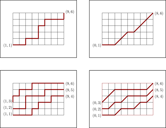
Figure 29. Paths and tuples of paths that contribute to the polymer partition functions: $R^{5}_{1}(9)$ (top left), $R^{5}_{3}(9)$ (bottom left), $L^{6}_{1}(8)$ (top right), $L^{6}_{3}(8)$ (bottom right).

Distributions of ratios of the polymer partition functions defined above are sometimes called Whittaker processes (or, to be more precise, $\alpha$-Whittaker processes), cf. [7]. They arise as limits (as $q$, the $a_{j}$’s and the $\alpha_{t}$’s simultaneously go to $1$) of suitably rescaled particle positions in an interlacing integer array distributed according to the $q$-Whittaker process $\mathscr{M}_{\mathbf{A}}^{\vec{a}}$ (§2.3), where

$$\mathbf{A}=(\alpha_{1},\ldots,\alpha_{t}),\qquad{\vec{a}}=(a_{1},\ldots,a_{n}).$$

The convergence of $q$-Whittaker processes to Whittaker processes is known in the literature, see [7, Thm. 4.2.4]. Since both dynamics $\mathscr{Q}^{q}_{\textnormal{row}}[\alpha]$ and $\mathscr{Q}^{q}_{\textnormal{col}}[\alpha]$ constructed in §6 sample the $q$-Whittaker processes, we can employ them to give another proof of this limit transition. Moreover, we also establish the convergence of the corresponding stochastic dynamics.

Let us first define the appropriately scaled pre-limit dynamics. In what follows, for $\epsilon>0$ and $\theta_{j},\hat{\theta}_{t}$ as above, we set $q:=e^{-\epsilon}$, $a_{j}=e^{-\theta_{j}\epsilon}$ and $\alpha_{t}:=e^{-\hat{\theta}_{t}\epsilon}$.

Definition 8.4 (Scaled $\mathscr{Q}^{q}_{\textnormal{row}}[\alpha]$ dynamics).

Start the dynamics $\mathscr{Q}^{q}_{\textnormal{row}}[\alpha]$ from the zero initial condition (that is, $\lambda^{(j)}_{i}(0)\equiv 0$). Denote by $r_{j,k}(t,\epsilon)$ the position of the $k$-th particle from the right on the $j$-th level of the array after $t$ steps of the dynamics (at each time step $t\to t+1$, apply the dynamics $\mathscr{Q}^{q}_{\textnormal{row}}[\alpha]$ with parameter $\alpha=\alpha_{t+1}$). For $t\geq k$, define the random variables $\hat{R}^{j}_{k}(t,\epsilon)$ via

$$r_{j,k}(t,\epsilon)=(t+j-2k+1)\epsilon^{-1}\log\epsilon^{-1}+\epsilon^{-1}\log(\hat{R}^{j}_{k}(t,\epsilon)).$$

The reason for the restriction $t\geq k$ comes from the fact that $r_{j,k}(t,\epsilon)=0$ for $t<k$.

We will view the collection of random variables $\{\hat{R}^{j}_{k}(t,\epsilon)\}$ as a stochastic process $\hat{R}(t,\epsilon)$ which at a fixed time $t$ becomes an array $\hat{R}^{j}_{k}(t,\epsilon)$, $1\leq k\leq j\leq n$ for $t\geq n$, or a truncated array $\hat{R}^{j}_{k}(t,\epsilon)$, $1\leq k\leq\min\{t,j\}\leq n$ for $0<t<n$.

Definition 8.5 (Scaled $\mathscr{Q}^{q}_{\textnormal{col}}[\alpha]$ dynamics).

Start the dynamics $\mathscr{Q}^{q}_{\textnormal{col}}[\alpha]$ from the zero initial condition, and denote by $\ell_{j,k}(t,\epsilon)$ the position of the $k$-th particle from the left on the $j$-th level of the array after $t$ steps of the dynamics (again, at each time step $t\to t+1$, apply the dynamics $\mathscr{Q}^{q}_{\textnormal{col}}[\alpha]$ with parameter $\alpha=\alpha_{t+1}$). For $t\geq j-k+1$, define the random variable $\hat{L}^{j}_{k}(t,\epsilon)$ via

$$\ell_{j,k}(t,\epsilon)=(t-j+2k-1)\epsilon^{-1}\log\epsilon^{-1}-\epsilon^{-1}\log(\hat{L}^{j}_{k}(t,\epsilon)).$$

The reason for the restriction $t\geq j-k+1$ comes from the fact that $\ell_{j,k}(t,\epsilon)=0$ for $t<j-k+1$.

We will view the collection of random variables $\{\hat{L}^{j}_{k}(t,\epsilon)\}$ as a stochastic process $\hat{L}(t,\epsilon)$, which at a fixed time $t$ becomes an array $\hat{L}^{j}_{k}(t,\epsilon)$, $1\leq k\leq j\leq n$ for $t\geq n$, or a truncated array $\hat{L}^{j}_{k}(t,\epsilon)$, $1\leq k\leq j\leq\min\{n,k+t-1\}$ for $0<t<n$.

Remark 8.6.

Observe that for a fixed time $t$, the array $r_{j,k}(t,\epsilon)$ has the same distribution as the array $\ell_{j,j-k+1}(t,\epsilon)$ (by Theorems 6.4 and 6.11, they are distributed as $q$-Whittaker processes). Hence the (possibly truncated) arrays $\hat{R}^{j}_{k}(t,\epsilon)$ and $1/\hat{L}^{j}_{j-k+1}(t,\epsilon)$ for $1\leq k\leq\min\{t,j\}\leq n$ have the same distribution. However, these arrays will not be identically distributed as stochastic processes in $t$ since they come from different multivariate dynamics.

In the setting of polymer partition functions, define random processes $\hat{R}(t)$ and $\hat{L}(t)$ on (possibly truncated) arrays via

$$\hat{R}^{j}_{k}(t):=R^{j}_{k}(t)/R^{j}_{k-1}(t),\quad\text{for $1\leq k\leq\min\{t,j\}\leq n$}$$

and

$$\hat{L}^{j}_{k}(t):=L^{j}_{k}(t)/L^{j}_{k-1}(t),\quad\text{for $1\leq k\leq j\leq\min\{n,k+t-1\}$}.$$

They are well defined, because $R^{j}_{k}(t),R^{j}_{k-1}(t)>0$ for $t\geq k$ and $L^{j}_{k}(t),L^{j}_{k-1}(t)>0$ for $t\geq j-k+1$.

We are now in a position to formulate results on the limiting behavior of dynamics $\mathscr{Q}^{q}_{\textnormal{row}}[\alpha]$ and $\mathscr{Q}^{q}_{\textnormal{col}}[\alpha]$. In this section we prove the following:

Theorem 8.7.

As $\epsilon\to 0$, the process $\hat{R}(t,\epsilon)$ of Definition 8.4 converges in distribution to the process $\hat{R}(t)$.

Theorem 8.8.

As $\epsilon\to 0$, the process $\hat{L}(t,\epsilon)$ of Definition 8.5 converges in distribution to the process $\hat{L}(t)$.

Corollary 8.9.

The (possibly truncated) arrays $\hat{R}^{j}_{k}(t)$ and $1/\hat{L}^{j}_{j-k+1}(t)$ for $1\leq k\leq\min\{t,j\}\leq n$ have the same distribution.

In particular, $1/\hat{R}^{j}_{j}(t)$ and $\hat{L}^{j}_{1}(t)$ have the same distribution. The latter fact was proven in [58], and was used to analyze the strict-weak polymer partition function via the geometric RSK row insertion (see §8.2.1 below), and to establish the Tracy-Widom asymptotics for the strict-weak polymer.

See also [58] for the close relation between the log-gamma and strict-weak polymers, where it is explained that one is the complement of the other at the level of lattice paths. To the best of our knowledge, the full statement of Corollary 8.9 has not previously appeared in the literature.

Let us provide a brief outline of our proofs of Theorems 8.7 and 8.8 which are presented in the rest of this section. First, in §8.2 we describe the constructions of the geometric RSK correspondences, which will serve as $\epsilon\to 0$ limits of elementary steps used in dynamics $\mathscr{Q}^{q}_{\textnormal{row}}[\alpha]$ and $\mathscr{Q}^{q}_{\textnormal{col}}[\alpha]$. Then in §8.3 we prove a number of lemmas concerning $\epsilon\to 0$ behavior of the $q$-distributions from §6.1. Finally, in §8.4 we use these ingredients to establish the desired statements.

8.2. Geometric RSKs

As we already know, the dynamics on $q$-Whittaker processes constructed in §6 degenerate for $q=0$ into the dynamics $\mathscr{Q}^{q=0}_{\textnormal{row}}[\alpha]$ and $\mathscr{Q}^{q=0}_{\textnormal{col}}[\alpha]$ based on the classical RSK row or column insertion, respectively. In this subsection we describe the corresponding geometric Robinson–Schensted–Knuth insertions, which will serve as building blocks for understanding $q\nearrow 1$ limits of the dynamics on $q$-Whittaker processes.

The $q=0$ and $q\nearrow 1$ pictures (i.e., the classical and the geometric RSK correspondences) are related via a certain procedure called detropicalization. Namely, the geometric RSK row insertion introduced in [44] is obtained by detropicalizing the classical RSK row insertion by replacing the $(\max,+)$ operations in its definition by $(+,\times)$. About the geometric RSK row insertion see also, e.g., [53], [22], [60], and [19].

By analogy with the geometric RSK row insertion, one can define the geometric RSK column insertion, by detropicalizing the classical RSK column insertion, this time replacing the $(\min,+)$ operations by $(+,\times)$.

Remark 8.10 (Names and notation).

The geometric RSK correspondences are also sometimes called tropical RSK correspondences [44], [53], [22], despite the fact that they come from the process of detropicalization. We adopt a convention of calling them the geometric RSK correspondences (following, e.g., [60], [19], [57]). The latter name arises in connection with geometric crystals (see [19] for more background).

Note that the word “geometric” in the name of the geometric RSK correspondences should be distinguished from the same word in the names of the geometric $q$-PushTASEP and the geometric $q$-TASEP (described in §6.3 and §6.6, respectively). The former refers to detropicalization of the classical RSK correspondences, while the latter is attached to the $q$-geometric jump distribution.

Below in this section, by $\lambda,\nu,\ldots$ we will denote vectors (words) with continuous components, and not signatures as before. To indicate the difference, we will use superscripts to denote their components.

8.2.1. Geometric RSK row insertion

Consider a triangular array $z^{j}_{k}$ ($1\leq k\leq j\leq n$) of nonnegative real numbers, such that a word $z_{k}=(z^{k}_{k},\ldots,z^{n}_{k})$ either has all positive entries or is equal to $(1,0,\ldots,0)$ (in which case we call it an empty word).

First, define the geometric row insertion of a nonempty word $a=(a^{k},\ldots,a^{n})$ into a nonempty word $\lambda=(\lambda^{k},\ldots,\lambda^{n})$ as an operation that takes the pair $\{\lambda,a\}$ as input, and produces a pair of words $\{\nu=(\nu^{k},\ldots,\nu^{n}),b=(b^{k+1},\ldots,b^{n})\}$ as output via the following rule:

If $\lambda$ is an empty word, then by definition $b$ is not produced, while

$$\nu:=(a^{k},a^{k}a^{k+1},\ldots,a^{k}a^{k+1}\cdots a^{n})$$

is produced according to the same rule. The word $b$ is also not produced for $k=n$. Observe that always $\nu^{j}=(\lambda^{j}+\nu^{j-1})a^{j}$ for $k<j\leq n$ and $\nu^{k}=\lambda^{k}a^{k}$.

Figure 30. Geometric RSK row insertion.

Definition 8.11.

The geometric RSK row insertion of a word $a=(a^{1},\ldots,a^{n})$ into an array $z^{j}_{k}$ is defined by consecutively modifying the words $z_{1},\ldots,z_{n}$ via the insertion according to the diagram on Fig. 30. The bottom output word $a(1),a(2),\ldots$ of each insertion is then used as a top input word for the next insertion. If after some insertion no bottom output word is produced, then no further insertions are performed.

Figure 31. Array and strip for the geometric RSK row insertion.

The geometric RSK row insertion is related to the polymer partition functions of §8.1 in the following way:

Proposition 8.12 ([53]).

If we start with an array $z$ of empty words, and consecutively insert into it nonempty fixed words $a_{1},\ldots,a_{t}$, $a_{i}=(a_{i}^{1},\ldots,a_{i}^{n})$, via the geometric RSK row insertion, then in the obtained array we have

$$z^{j}_{k}(t)=\frac{R^{j}_{k}(t)(a_{1},\ldots,a_{t})}{R^{j}_{k-1}(t)(a_{1},\ldots,a_{t})}\qquad\text{for all $t\geq k$.}$$

Here with a slight abuse of notation we denote by $R^{j}_{k}(t)(a_{1},\ldots,a_{t})$ the same weighted sum over $k$-tuples of nonintersecting paths as in Definition 8.2, but in a strip in which each node $(s,i)$ has a deterministic weight $a^{i}_{s}$ (see Fig. 31).

8.2.2. Geometric RSK column insertion

Consider a triangular array $y^{j}_{k}$ ($1\leq k\leq j\leq n$) of nonnegative real numbers, such that in each word $y_{k}=(y^{k}_{k},\ldots,y^{n}_{k})$ either all entries are positive, or there is $k\leq j\leq n$, such that $y^{j}_{k}=1$, $y^{i}_{k}=0$ for $j<i\leq n$ and $y^{i}_{k}>0$ for $k\leq i\leq j$. We again call $(1,0,\ldots,0)$ an empty word.

To define the geometric RSK column insertion first define the insertion of a word $a=(a^{k},\ldots,a^{n})$ with positive entries into a word $\lambda=(\lambda^{k},\ldots,\lambda^{n})$ as an operation that takes the pair $\{\lambda,a\}$ as input, and produces a pair of words $\{\nu=(\nu^{k},\ldots,\nu^{n}),b=(b^{k+1},\ldots,b^{n})\}$ as output via the following rule:

Definition 8.13.

The geometric RSK column insertion of a word into an array is defined similarly to the row insertion (Definition 8.11), by consecutively performing the column insertion operations defined above, in order as on Fig. 30.

Figure 32. Array and strip for the geometric RSK column insertion.

Note that $y^{j}_{k}$ in this definition corresponds to $\lambda^{(j)}_{j-k+1}$ in the classical RSK column insertion. We will need the following fact which is analogous to Proposition 8.12:

Proposition 8.14.

If we start with an array $y$ of empty words, and consecutively insert into it words $a_{1},\ldots,a_{t}$ with positive entries via the geometric RSK column insertion, then in the obtained array we have

$$y^{j}_{k}(t)=\frac{L^{j}_{k}(t)(a_{1},\ldots,a_{t})}{L^{j}_{k-1}(t)(a_{1},\ldots,a_{t})}\qquad\text{for all $t\geq j-k+1$}.$$

Here again we denote by $L^{j}_{k}(t)(a_{1},\ldots,a_{t})$ the same weighted sum over $k$-tuples of nonintersecting paths as in Definition 8.3, but in a strip in which each edge $(s-1,i)\to(s,i)$ has a deterministic weight $a^{i}_{s}$ (see Fig. 32).

Proof.

Our proof is similar to that of Proposition 8.12 (the latter is given in [53]).

For $a=(a^{1},\ldots,a^{n})$, denote by $H(a)$ the $n\times n$ matrix such that $H(a)_{i,i}:=a^{i}$, $H(a)_{i,i+1}=1$, and other entries are $0$. For $a=(a^{k},\ldots,a^{n})$, denote by $H_{k}(a)$ the $n\times n$ matrix of the form $\left(\begin{array}[]{cc}Id_{k-1}&0\\ 0&H(a)\end{array}\right).$ For $\lambda=(\lambda^{k},\ldots,\lambda^{n})$ such that $\lambda^{i}>0$ for $k\leq i\leq j$ and $\lambda^{i}=0$ for $j<i\leq n$, denote by $G(\lambda)$ the $n\times n$ matrix of the form

$$\left(\begin{array}[]{ccc}Id_{k-1}&0&0\\ 0&G&0\\ 0&0&Id_{n-j}\end{array}\right),$$

where $G$ is the upper-triangular $(j-k+1)\times(j-k+1)$ matrix with

$$G_{p,r}=\frac{\lambda^{r+k-1}}{\lambda^{p+k-2}}\quad\text{for $1\leq p\leq r\leq j-k+1$.}$$

Assume $\lambda^{k-1}=1$.

The key to the proof is the commutation relation

$$G(\lambda)H_{k}(a)=H_{k+1}(b)G(\nu),$$ (8.3)

whenever a pair of words $\nu=(\nu^{k},\ldots,\nu^{n}),b=(b^{k+1},\ldots,b^{n})$ is obtained by inserting $a=(a^{k},\ldots,a^{n})$ into $\lambda=(\lambda^{k},\ldots,\lambda^{n})$.

To check (8.3), denote its left-hand side by $\mathsf{L}$ and right-hand side by $\mathsf{R}$. Clearly, $\mathsf{L}_{i,i}=\mathsf{R}_{i,i}=1$ for $1\leq i\leq k-1$ and $\mathsf{L}_{i,i}=\mathsf{R}_{i,i}=a^{i}$ for $j+2\leq i\leq n$, and $\mathsf{L}_{j+1,j+2}=\mathsf{R}_{j+1,j+2}=1$. Otherwise $\mathsf{L}_{i,m}=\mathsf{R}_{i,m}=0$ unless $k\leq i\leq j+1$ and $k\leq m\leq j+1$. Let us thus assume that the two latter inequalities hold. On the diagonal, for $k<i<j+1$, we have

$$\mathsf{L}_{i,i}=a^{i}\frac{\lambda^{i}}{\lambda^{i-1}}=b^{i}\frac{\nu^{i}}{\nu^{i-1}}=\mathsf{R}_{i,i},\qquad\mathsf{L}_{k,k}=a^{k}\lambda^{k}=\nu^{k}=\mathsf{R}_{k,k},$$

and

$$\mathsf{L}_{j+1,j+1}=a^{j+1}=\frac{b^{j+1}}{\nu^{j}}=\mathsf{R}_{j+1,j+1}.$$

Above the diagonal, for $k<i<m\leq j+1$, we have

$$\mathsf{L}_{i,m}=\frac{\lambda^{m-1}}{\lambda^{i-1}}+\frac{\lambda^{m}}{\lambda^{i-1}}a^{m}=\frac{\nu^{m}}{\lambda^{i-1}}=b^{i}\frac{\nu^{m}}{\nu^{i-1}}+\frac{\nu^{m}}{\nu^{i}}=\mathsf{R}_{i,m},$$

since $\frac{b^{i}}{\nu^{i-1}}+\frac{1}{\nu^{i}}=\frac{1}{\nu^{i}}(a^{i}\frac{\lambda^{i}}{\lambda^{i-1}}+1)=\frac{1}{\lambda^{i-1}}$, and finally

$$\mathsf{L}_{k,m}=\lambda^{m-1}+\lambda^{m}a^{m}=\nu^{m}=\mathsf{R}_{k,m}.$$

This completes the proof of the commutation relation (8.3).

By applying the commutation relation multiple times according to the geometric column RSK insertion (Definition 8.13), we get

$$G(y_{n}(t))\cdot\cdots\cdot G(y_{1}(t))=H(a_{1})\cdot\cdots\cdot H(a_{t}).$$ (8.4)

Observe that the $(i,j)$-entry of the right-hand side above is equal to the sum of weights of all directed strict-weak (as on Fig. 29, right) paths from $(0,i)$ to $(t,j)$, where the weight of a path is given by the product of weights of horizontal edges, as before. Indeed, this entry is equal to

$$\sum_{1\leq i_{1},\ldots,i_{t+1}\leq n:\ i_{1}=i,i_{t+1}=j}\prod_{\ell=1}^{t}H(a_{\ell})_{i_{\ell},i_{\ell+1}}=\sum_{1\leq i_{1},\ldots,i_{t+1}\leq n:i_{1}=i,i_{t+1}=j}\prod_{\ell=1}^{t}(\mathbf{1}_{i_{\ell}=i_{\ell+1}-1}+a_{\ell}\mathbf{1}_{i_{\ell}=i_{\ell+1}}).$$

By the Lindström-Gessel-Viennot principle [51], [39], the determinant of the minor of the right-hand side at the intersection of the first $k$ rows, and columns from $(j-k+1)$-st to $j$-th, is $L^{j}_{k}(t)(a_{1},\ldots,a_{t})$.

Next, observe that for $1\leq s\leq k$, $j-k+1\leq p\leq j$, the $(s,p)$-entry of the left-hand side of (8.4) is equal to the sum of weights of directed up/right (as on Fig. 29, left) lattice paths from $(k+1-s,s)$ to $(\min\{k+t+1-p,k\},p)$ in the array as on Fig. 33 (the left picture if $t\geq j$, and the right one if $j-k+1\leq t<j$).

Figure 33. Arrays used in the proof of Proposition 8.14.

The weight of each path is defined to be the product of weights of all nodes along the path. By Lindström-Gessel-Viennot principle, the determinant of the minor of the left-hand side of (8.4) at the intersection of the first $k$ rows, and columns from $(j-k+1)$-st to $j$-th, is equal to the sum of weights of all $k$-tuples of nonintersecting paths from $(k,1),\ldots,(2,k-1),(1,k)$ to ${(\min\{2k+t-j,k\},j-k+1)},\ldots,$ ${(\min\{k+t+2-j,k\},j-1)},$ ${(\min\{k+t+1-j,k\},j)}$. There is only one such tuple, which covers all points on Fig. 33 and has weight $\displaystyle\prod_{i=1}^{k}y^{\min\{i+t,j\}}_{i}$.

Therefore,

$$\displaystyle L^{j}_{k}(t)(a_{1},\ldots,a_{t})=\prod_{i=1}^{k}y^{\min\{i+t,j\}}_{i},\qquad t\geq j-k+1,$$

which establishes the desired statement. ∎

8.3. Asymptotics of $q$-deformed Beta-binomial distributions

We will need several lemmas about the limiting properties of the distributions $\boldsymbol{\varphi}_{q,\xi,\eta}(s\mid y)$ (6.1).

Lemma 8.15.

Let $X^{\epsilon}$ be a $\mathbb{Z}_{\geq 0}$-valued random variable with

$$Prob(X^{\epsilon}=j)=(\alpha;q)_{\infty}\frac{\alpha^{j}}{(q;q)_{j}}\quad\text{for $\alpha=e^{-\theta\epsilon}$ and $q=e^{-\epsilon}$.}$$

Then as $\epsilon\to 0$, $\epsilon\exp\{\epsilon X^{\epsilon}\}$ converges in distribution to $\mathop{\mathrm{Gamma}^{-1}}(\theta)$.

Lemma 8.16.

Let $n(\epsilon)$ be a function $\mathbb{R}_{\geq 0}\to\mathbb{Z}_{\geq 0}$, such that

$$\lim_{\epsilon\to 0}\epsilon^{-1}\exp\{-\epsilon n(\epsilon)\}=\varphi.$$

Let $X^{\epsilon}$ be a $\mathbb{Z}_{\geq 0}$-valued random variable with

$$Prob(X^{\epsilon}=j)=\boldsymbol{\varphi}_{q,\alpha,0}(j\mid n(\epsilon))\quad\text{for $\alpha=e^{-\theta\epsilon}$ and $q=e^{-\epsilon}$.}$$

Then as $\epsilon\to 0$, $\epsilon^{-1}\exp\{-\epsilon X^{\epsilon}\}$ converges in distribution to $\varphi\ +$ $\mathop{\mathrm{Gamma}}(\theta)$.

These two lemmas were both proven in [25] (Lemma 2.1 and a part of proof of Theorem 1.4, respectively). In the next three lemmas, parameters of distributions which are not explicitly fixed are assumed to depend on $\epsilon$, and sometimes might also be random themselves.

Lemma 8.17.

Fix $C$ and $0<\sigma<1$. Let $Y^{\epsilon}$ be a $\mathbb{Z}_{\geq 0}$-valued random variable distributed according to $\boldsymbol{\varphi}_{q^{-1},\xi,\eta}(\cdot\mid n)$ with $q=e^{-\epsilon}$, $\xi q^{-n}\to\sigma$, $n\geq\epsilon^{-1}\log\epsilon^{-1}-\epsilon^{-1}C$, and $\log\eta+2n\epsilon\leq\log\sigma$. Then as $\epsilon\to 0$, $\epsilon Y^{\epsilon}\to\log(1+\sigma)$.

Proof.

The fact that $\boldsymbol{\varphi}_{q^{-1},\xi,\eta}$ with such parameters is indeed a probability distribution for $\epsilon$ small enough follows from inequalities in the statement of the lemma. Let $A(\epsilon):=(e^{-\epsilon};e^{-\epsilon})_{\infty}$. By [7, Corollary 4.1.10],

$$(e^{-\epsilon};e^{-\epsilon})_{\lfloor\epsilon^{-1}\log\epsilon^{-1}-C\epsilon^{-1}\rfloor}\leq A(\epsilon)C^{\prime}$$

for all $\epsilon$ small enough and some constant $C^{\prime}$ that depends only on $C$. As $\epsilon\to 0$,

$$\epsilon\log(e^{-\epsilon};e^{-\epsilon})_{\lceil r/\epsilon\rceil}\to\int_{0}^{r}\log(1-e^{-x})dx,$$

since the left-hand side is a Riemann sum for the right-hand side integral, hence we have

$$\epsilon\log\frac{(e^{-\epsilon};e^{-\epsilon})_{\infty}}{(e^{-r};e^{-\epsilon})_{\infty}}\to\int_{0}^{r}\log(1-e^{-x})dx.$$

(Note that although this integral blows up at $0$, it is still finite and convergence holds.)

Fix $\delta>0$. For $\epsilon$ small enough,

$$Prob(Y^{\epsilon}=k) =(\xi q^{-n+k})^{k}\frac{({\eta}/{\xi};q^{-1})_{k}(\xi;q^{-1})_{n-k}}{(\eta;q^{-1})_{n}}\binom{n}{k}_{q}\leq\frac{(\xi q^{-n})^{k}e^{-\epsilon k^{2}}C^{\prime}}{(e^{-\epsilon};e^{-\epsilon})_{k}}$$

$$\leq\frac{(2\sigma)^{k}e^{-\epsilon k^{2}}C^{\prime}}{(e^{-\epsilon};e^{-\epsilon})_{k}}\leq C^{\prime}\exp\left(k\log 2\sigma-\epsilon k^{2}-\frac{1}{\epsilon}\int_{0}^{k\epsilon}\log(1-e^{-x})dx\right)$$

$$\leq e^{-T^{2}/2\epsilon}\quad\text{for $T$ large enough and $k\geq T/\epsilon$.}$$

Hence

$$Prob(Y^{\epsilon}\geq T/\epsilon)\leq\sum_{k=\lceil T/\epsilon\rceil}^{\infty}e^{-\epsilon k^{2}/2}\leq e^{-T^{2}/2\epsilon}\sum_{i=0}^{\infty}e^{-Ti},$$

which can be made less than $\delta/2$ for all $\epsilon$ small enough by choosing sufficiently large $T$.

Observe that for $k\leq T/\epsilon$ and $\epsilon$ small enough there is some constant $C_{0}$ that depends only on $C$ and $T$, such that

$$C_{0}^{-1}\leq\frac{({\eta}/{\xi};q^{-1})_{k}}{(\xi q;q)_{\infty}(\eta;q^{-1})_{n}}\frac{(q;q)_{n}}{(q;q)_{n-k}}\leq C_{0}.$$

Let

$$f(\psi):=-\psi^{2}+(\log\sigma)\psi-\int_{0}^{\psi}\log(1-e^{-x})dx-\int_{0}^{\psi-\log\sigma}\log(1-e^{-x})dx$$

for $\psi\geq 0$. Then

$$f^{\prime}(\psi)=-2\psi+\log\sigma-\log(1-e^{-\psi})-\log(1-e^{-\psi+\log\sigma}),$$

which is strictly decreasing, and $f^{\prime}(\log(1+\sigma))=0$. Hence $f$ attains a unique maximum at $\log(1+\sigma)$, so one can choose $M_{1}>M_{2}>M_{3}>M_{4}$ such that

$$f(\psi)>M_{1}\quad\text{for $\psi\in(\log(1+\sigma)-\delta/2,\log(1+\sigma)+\delta/2)$}$$

and

$$f(\psi)<M_{4}\quad\text{for $\psi\notin(\log(1+\sigma)-\delta,\log(1+\sigma)+\delta)$,}$$

and for $\epsilon$ small enough

$$Prob(\epsilon Y^{\epsilon}\in(\log(1+\sigma)-\delta/2,\log(1+\sigma)+\delta/2))\geq C_{0}^{-1}\left(\frac{\delta}{\epsilon}-1\right)A(\epsilon)e^{M_{2}/\epsilon}$$

and

$$Prob(\epsilon Y^{\epsilon}\notin(\log(1+\sigma)-\delta,\log(1+\sigma)+\delta)\cup[T,\infty))\leq C_{0}\left(\frac{T-2\delta}{\epsilon}+2\right)A(\epsilon)e^{M_{3}/\epsilon}.$$

Therefore, for $\epsilon$ small enough

$$Prob(\epsilon Y^{\epsilon}\in(\log(1+\sigma)-\delta,\log(1+\sigma)+\delta))\geq 1-\delta,$$

and this completes the proof. ∎

Lemma 8.18.

Fix $C$ and $0\leq\sigma<1$. Let $Y^{\epsilon}$ be a $\mathbb{Z}_{\geq 0}$-valued random variable with

$$Prob(Y^{\epsilon}=j)=\boldsymbol{\varphi}_{q,\alpha,0}(j\mid n)$$

for $\alpha\to\sigma$ as $\epsilon\to 0$, $q=e^{-\epsilon}$ and $n\geq\epsilon^{-1}\log\epsilon^{-1}-\epsilon^{-1}C$. Then as $\epsilon\to 0$, $\epsilon Y^{\epsilon}\to-\log(1-\sigma)$.

Proof.

Suppose $\sigma>0$ and fix $\delta>0$. We can write

$$Prob(Y^{\epsilon}=k)=\frac{\alpha^{k}}{(e^{-\epsilon};e^{-\epsilon})_{k}}\frac{(\alpha;e^{-\epsilon})_{n-k}(e^{-\epsilon},e^{-\epsilon})_{n}}{(e^{-\epsilon};e^{-\epsilon})_{n-k}}\leq\frac{\alpha^{k}}{(e^{-\epsilon};e^{-\epsilon})_{k}}$$

$$\hskip 100.0pt\leq\exp\left(\frac{1}{\epsilon}((\frac{1}{2}\log\sigma)T-\int_{0}^{T}\log(1-e^{-x})dx)\right)\leq e^{(\log\sigma)T/4\epsilon}$$

for $T$ large enough and $\epsilon$ small enough, such that $k\geq T/\epsilon$. Hence

$$Prob(Y^{\epsilon}\geq T/\epsilon)\leq e^{(\log\sigma)T/4\epsilon}\sum_{i=0}^{\infty}e^{\frac{i\log\sigma}{4}}$$

which is less than $\delta/2$ for $T$ large enough.

For $\epsilon$ small enough, $k\leq T/\epsilon$, and some constant $C_{0}$ that depends only on $C$, $T$, and $\sigma$, one can write

$$C_{0}^{-1}(\alpha;e^{-\epsilon})_{\infty}\leq\frac{(\alpha;e^{-\epsilon})_{n-k}(e^{-\epsilon};e^{-\epsilon})_{n}}{(e^{-\epsilon};e^{-\epsilon})_{n-k}}\leq C_{0}(\alpha;e^{-\epsilon})_{\infty}.$$

Let

$$f(\psi):=(\log\sigma)\psi-\int_{0}^{\psi}\log(1-e^{-x})dx$$

for $\psi\geq 0$. Then

$$f^{\prime}(\psi)=\log\sigma-\log(1-e^{-\psi}),$$

which is strictly decreasing, and $f^{\prime}(-\log(1-\sigma))=0$. Hence $f$ attains a unique maximum at $-\log(1-\sigma)$, so one can choose $M_{1}>M_{2}>M_{3}>M_{4}$ such that

$$f(\psi)>M_{1}\quad\text{for $\psi\in(-\log(1-\sigma)-\delta/2,-\log(1-\sigma)+\delta/2)$}$$

and

$$f(\psi)<M_{4}\quad\text{for $\psi\notin(-\log(1-\sigma)-\delta,-\log(1-\sigma)+\delta)$,}$$

and for $\epsilon$ small enough

$$Prob(\epsilon Y^{\epsilon}\in(-\log(1-\sigma)-\delta/2,-\log(1-\sigma)+\delta/2))\geq C_{0}^{-1}\left(\frac{\delta}{\epsilon}-1\right)(\alpha;e^{-\epsilon})_{\infty}e^{M_{2}/\epsilon}$$

and

$$Prob(\epsilon Y^{\epsilon}\notin(-\log(1-\sigma)-\delta,-\log(1-\sigma)+\delta)\cup[T,\infty))\leq C_{0}\left(\frac{T-2\delta}{\epsilon}+2\right)(\alpha;e^{-\epsilon})_{\infty}e^{M_{3}/\epsilon}.$$

Therefore, for $\epsilon$ small enough we can write

$$Prob(\epsilon Y^{\epsilon}\in(-\log(1-\sigma)-\delta,-\log(1-\sigma)+\delta))\geq 1-\delta,$$

and this completes the proof for the case $\sigma>0$.

If $\sigma=0$, fix arbitrary $u>0$. For all large enough $U$, such that $Uu>\frac{1}{2}Uu-\int_{0}^{\infty}\log(1-e^{-x})dx$, $\epsilon$ small enough, and $k\geq\frac{u}{\epsilon}$,

$$Prob(Y^{\epsilon}=k)\leq\frac{\alpha^{k}}{(e^{-\epsilon};e^{-\epsilon})_{k}}\leq\exp\left(\frac{1}{\epsilon}(-Uk\epsilon-\int_{0}^{\infty}\log(1-e^{-x})dx)\right)\leq e^{-\frac{Uu}{2\epsilon}}.$$

So,

$$Prob(\epsilon Y^{\epsilon}\geq u)\leq e^{-\frac{Uu}{2\epsilon}}\sum_{i=0}^{\infty}e^{-Ui/2},$$

which can be made less than any given $\delta>0$ for $U$ large enough. Thus, we have convergence $\epsilon Y^{\epsilon}\to 0$ in distribution. ∎

Lemma 8.19.

Fix $\alpha,\sigma\in(0,1)$ such that $\alpha(1+\sigma)<1$. Let $Y^{\epsilon}$ be a $\mathbb{Z}_{\geq 0}$-valued random variable with $Prob(Y^{\epsilon}=j)=\boldsymbol{\varphi}_{q^{-1},\alpha,0}(j\mid n)$ for ${n\epsilon\to\log(1+\sigma)}$ as $\epsilon\to 0$, $q=e^{-\epsilon}$. Then as $\epsilon\to 0$, $\epsilon Y^{\epsilon}\to\log(1+\alpha\sigma)$.

Proof.

$\alpha(1+\sigma)<1$ ensures that this is indeed a probability distribution for $\epsilon$ small enough. This distribution looks as

$$Prob(Y^{\epsilon}=k)=\frac{(q;q)_{n}}{(q;q)_{k}(q;q)_{n-k}}(\alpha q^{k-n})^{k}(\alpha;q^{-1})_{n-k}.$$

Let

$$f(\psi) :=-\int_{0}^{\psi}\log(1-e^{-x})dx-\int_{0}^{\log(1+\sigma)-\psi}\log(1-e^{-x})dx+\psi\log\alpha-\psi^{2}+\psi\log(1+\sigma)$$

$$+\int_{-\log\alpha-\log(1+\sigma)+\psi}^{-\log\alpha}\log(1-e^{-x})dx\quad\text{for $\log(1+\sigma)\geq\psi\geq 0$.}$$

Then

$$f^{\prime}(\psi)=-\log(1-e^{-\psi})+\log(1-\frac{e^{\psi}}{1+\sigma})+\log\alpha-2\psi+\log(1+\sigma)-\log(1-\alpha(1+\sigma)e^{-\psi}),$$

which is strictly decreasing, and $f^{\prime}(\log(1+\alpha\sigma))=0$. Hence $f$ attains a unique maximum at $\log(1+\alpha\sigma)$, so one can choose $M_{1}>M_{2}$ such that

$$f(\psi)>M_{1}\quad\text{for $\psi\in(\log(1+\alpha\sigma)-\delta/2,\log(1+\alpha\sigma)+\delta/2)$}$$

and

$$f(\psi)<M_{2}\quad\text{for $\psi\notin(\log(1+\alpha\sigma)-\delta,\log(1+\alpha\sigma)+\delta)$.}$$

Hence for $\epsilon$ small enough,

$$Prob(\epsilon Y^{\epsilon}\in(\log(1+\alpha\sigma)-\delta/2,\log(1+\alpha\sigma)+\delta/2))\geq\left(\frac{\delta}{\epsilon}-1\right)(e^{-\epsilon};e^{-\epsilon})_{n}e^{M_{1}/\epsilon},$$

and

$$Prob(\epsilon Y^{\epsilon}\notin(\log(1+\alpha\sigma)-\delta,\log(1+\alpha\sigma)+\delta))\leq\left(\frac{\log(1+\sigma)-2\delta}{\epsilon}+2\right)(e^{-\epsilon};e^{-\epsilon})_{n}e^{M_{2}/\epsilon}.$$

Thus, for $\epsilon$ small enough, we have

$$Prob(\epsilon Y^{\epsilon}\in(\log(1+\alpha\sigma)-\delta,\log(1+\alpha\sigma)+\delta))\geq 1-\delta,$$

and this completes the proof. ∎

8.4. Proofs of Theorems 8.7 and 8.8

In our proofs, we denote by

$$A(\epsilon),B(\epsilon),C(\epsilon),D(\epsilon),E(\epsilon),F(\epsilon)$$

possibly random positive valued functions tending to deterministic constants $A,B,C,D,E,F$, respectively, as $\epsilon\to 0$. This notation will be repeatedly used in the arguments below for defining conditional probabilities.

8.4.1. Proof of Theorem 8.7

We must show that for fixed $(t,k,j)$, such that $k\leq\min\{t,j\}$ and $j\leq n$, the random variable $\hat{R}^{j}_{k}(t,\epsilon)$ conditioned on $\hat{R}^{J}_{K}(T,\epsilon)\to X^{J}_{K}(T)$ for all ${(T,K,J)<(t,k,j)}$ in the lexicographic order, converges as $\epsilon\to 0$ to $\hat{R}^{j}_{k}(t)$ conditioned on $\hat{R}^{J}_{K}(T)=X^{J}_{K}(T)$ for all ${(T,K,J)<(t,k,j)}$ in the lexicographic order. Here $X^{J}_{K}(T)$ are some fixed constants. In the rest of the proof we will always assume this conditioning.

Right edge ($k=1$). The Markovian projection of the $\mathscr{Q}^{q}_{\textnormal{row}}[\alpha]$ dynamics on the right edge is the geometric $q$-PushTASEP (§6.3), hence the proof of the theorem for the right edge is the same as showing that suitably rescaled positions of particles in the geometric $q$-PushTASEP converge to the partition functions of the log-Gamma polymer (Definition 8.2).

a) If $t=1$, then $r_{j,1}(1,\epsilon)=r_{j-1,1}(1,\epsilon)\ +$ an independent random movement $d$ distributed according to $\boldsymbol{\varphi}_{q,a_{j}\alpha_{1},0}(d\mid\infty)$ (assume $r_{0,1}(1,\epsilon)=0$ and $X^{0}_{1}(1)=1$). By Lemma 8.15,

$$\log(\hat{R}^{j}_{1}(1,\epsilon)) ={r_{j,1}(1,\epsilon)\epsilon-j\log\epsilon^{-1}}$$

$$={r_{j-1,1}(1,\epsilon)\epsilon-(j-1)\log\epsilon^{-1}}+d\epsilon-\log\epsilon^{-1}$$

$$\to\log(X^{j-1}_{1}(1))+\log(\Gamma)$$

for an independent random variable $\Gamma=a^{j}_{1}$ distributed according to $\mathop{\mathrm{Gamma}^{-1}}(\theta_{j}+\hat{\theta}_{1})$, which is consistent with $\hat{R}^{j}_{1}(1)=X^{j-1}_{1}(1)a^{j}_{1}$.

b) If $j=1$ and $t\geq 2$, then $r_{1,1}(t,\epsilon)={r_{1,1}(t-1,\epsilon)}\ +$ an independent random movement $d$ distributed according to $\boldsymbol{\varphi}_{q,a_{1}\alpha_{t},0}(d\mid\infty)$. By Lemma 8.15,

$$\log(\hat{R}^{1}_{1}(t,\epsilon)) =r_{1,1}(t,\epsilon)\epsilon-t\log\epsilon^{-1}$$

$$=r_{1,1}(t-1,\epsilon)\epsilon-(t-1)\log\epsilon^{-1}+d\epsilon-\log\epsilon^{-1}$$

$$\to\log(X^{1}_{1}(t-1))+\log(\Gamma)$$

for an independent random variable $\Gamma=a^{1}_{t}$ distributed according to $\mathop{\mathrm{Gamma}^{-1}}(\theta_{1}+\hat{\theta}_{t})$, which is consistent with $\hat{R}^{1}_{1}(t)=X^{1}_{1}(t-1)a^{1}_{t}$.

c) Assume $t\geq 2$ and $j\geq 2$. Condition on

$$r_{j,1}(t-1,\epsilon)=(t+j-2)\epsilon^{-1}\log\epsilon^{-1}+\epsilon^{-1}\log A(\epsilon),\quad\text{so $X^{j}_{1}(t-1)=A$};$$

$$r_{j-1,1}(t-1,\epsilon)=(t+j-3)\epsilon^{-1}\log\epsilon^{-1}+\epsilon^{-1}\log B(\epsilon),\quad\text{so $X^{j-1}_{1}(t-1)=B$};$$

$$r_{j-1,1}(t,\epsilon)=(t+j-2)\epsilon^{-1}\log\epsilon^{-1}+\epsilon^{-1}\log C(\epsilon),\quad\text{so $X^{j-1}_{1}(t)=C$}.$$

The movement of the rightmost particle on the $j$-th level during the time step ${t-1\to t}$ which happens due to the pushing by the rightmost particle at level $j-1$ behaves as $\epsilon^{-1}\log(1+\frac{C}{A})$ (by Lemma 8.17). The independent movement of the rightmost particle on the $j$-th level behaves as $\epsilon^{-1}\log\Gamma+\epsilon^{-1}\log\epsilon^{-1}$ (by Lemma 8.15), for an independent random variable $\Gamma=a^{j}_{t}$ distributed according to $\mathop{\mathrm{Gamma}^{-1}}(\theta_{j}+\hat{\theta}_{t})$. Therefore,

$$\log(\hat{R}^{j}_{1}(t,\epsilon))\to\log A+\log(1+\frac{C}{A})+\log\Gamma=\log((A+C)\Gamma),$$

which is consistent with $\hat{R}^{j}_{1}(t)=(X^{j}_{1}(t-1)+X^{j-1}_{1}(t))a^{j}_{t}$.

$k$-th edge from the right for $k\geq 2$.

a) Assume $t=k$. We have $r_{j,k}(k,\epsilon)=r_{j-1,k}(k,\epsilon)\ +$ a movement due to pulling from the $(k-1)$-st particle from the right on the $(j-1)$-st level (assume $r_{k-1,k}(k,\epsilon)=0$ and $X^{k-1}_{k}(k)=1$). Condition on

$$r_{j-1,k-1}(k-1,\epsilon)=(j-k+1)\epsilon^{-1}\log\epsilon^{-1}+\epsilon^{-1}\log D(\epsilon),\quad\text{so $X^{j-1}_{k-1}(k-1)=D$};$$

$$r_{j-1,k-1}(k,\epsilon)=(j-k+2)\epsilon^{-1}\log\epsilon^{-1}+\epsilon^{-1}\log E(\epsilon),\quad\text{so $X^{j-1}_{k-1}(k)=E$};$$

$$r_{j,k-1}(k-1,\epsilon)=(j-k+2)\epsilon^{-1}\log\epsilon^{-1}+\epsilon^{-1}\log F(\epsilon),\quad\text{so $X^{j}_{k-1}(k-1)=F$}.$$

By Lemma 8.17, this movement times $\epsilon$ and minus $\log\epsilon^{-1}$ converges to ${\log({E}/{D})-\log(1+{E}/{F})}$. Therefore,

$$\log(\hat{R}^{j}_{k}(k,\epsilon)) =r_{j,k}(k,\epsilon)\epsilon-(j-k+1)\log\epsilon^{-1}$$

$$\to\log(X^{j-1}_{k}(k))+\log({E}/{D})-\log(1+{E}/{F})$$

$$=\log\left(\frac{X^{j-1}_{k}(k)EF}{(F+E)D}\right),$$

which is consistent with

$$\hat{R}^{j}_{k}(k)=\frac{X^{j-1}_{k}(k)X^{j-1}_{k-1}(k)X^{j}_{k-1}(k-1)}{\left(X^{j}_{k-1}(k-1)\ +\ X^{j-1}_{k-1}(k)\right)X^{j-1}_{k-1}(k-1)}.$$

Indeed, if we insert (via the geometric row insertion) a nonempty word ${b=(b^{k},\ldots,b^{n})}$ into the empty word $\lambda_{k}=(1,0,\ldots,0)$, where $b$ is itself the bottom output of the insertion of $a=(a^{k-1},\ldots,a^{n})$ into $\lambda_{k-1}=(\lambda^{k-1}_{k-1},\ldots,\lambda^{n}_{k-1})=(X^{k-1}_{k-1}(k-1),\ldots,X^{n}_{k-1}(k-1))$, then we get

$$\nu^{j}_{k}=\nu^{j-1}_{k}b^{j}=\nu^{j-1}_{k}\frac{a^{j}\lambda_{k-1}^{j}\nu_{k-1}^{j-1}}{\lambda_{k-1}^{j-1}\nu_{k-1}^{j}}={\nu^{j-1}_{k}\frac{\lambda_{k-1}^{j}}{\lambda_{k-1}^{j-1}}\cdot\frac{\nu^{j-1}_{k-1}}{\nu^{j-1}_{k-1}+\lambda^{j}_{k-1}}},$$

which is the same as the expression for $\hat{R}^{j}_{k}(k)$ above.

b) Assume $t\geq k+1$ and $k<j\leq n$. Condition on

$$r_{j,k}(t-1,\epsilon)=(t+j-2k)\epsilon^{-1}\log\epsilon^{-1}+\epsilon^{-1}\log A(\epsilon),\quad\text{so $X^{j}_{k}(t-1)=A$};$$

$$r_{j-1,k}(t-1,\epsilon)=(t+j-2k-1)\epsilon^{-1}\log\epsilon^{-1}+\epsilon^{-1}\log B(\epsilon),\quad\text{so $X^{j-1}_{k}(t-1)=B$};$$

$$r_{j-1,k}(t,\epsilon)=(t+j-2k)\epsilon^{-1}\log\epsilon^{-1}+\epsilon^{-1}\log C(\epsilon),\quad\text{so $X^{j-1}_{k}(t)=C$};$$

$$r_{j-1,k-1}(t-1,\epsilon)=(t+j-2k+1)\epsilon^{-1}\log\epsilon^{-1}+\epsilon^{-1}\log D(\epsilon),\quad\text{so $X^{j-1}_{k-1}(t-1)=D$};$$

$$r_{j-1,k-1}(t,\epsilon)=(t+j-2k+2)\epsilon^{-1}\log\epsilon^{-1}+\epsilon^{-1}\log E(\epsilon),\quad\text{so $X^{j-1}_{k-1}(t)=E$};$$

$$r_{j,k-1}(t-1,\epsilon)=(t+j-2k+2)\epsilon^{-1}\log\epsilon^{-1}+\epsilon^{-1}\log F(\epsilon),\quad\text{so $X^{j}_{k-1}(t-1)=F$}.$$

Movement of $r_{j,k}$ during time step ${t-1\to t}$ due to pushing by the $k$-th particle from the right on the $(j-1)$-st level behaves as $\epsilon^{-1}\log(1+\frac{C}{A})$ (by Lemma 8.17). The movement due to the pulling (by the $(k-1)$-st particle from the right on the $(j-1)$-st level) times $\epsilon^{-1}$ minus $\log\epsilon^{-1}$ by the same lemma tends to ${\log(\frac{E}{D})-\log(1+\frac{E}{F})}$. Hence we may write

$$\log(\hat{R}^{j}_{k}(t,\epsilon))\to\log A+\log\left(1+\frac{C}{A}\right)+\log\left(\frac{E}{D}\right)-\log\left(1+\frac{E}{F}\right)=\log\left(\frac{(A+C)EF}{(F+E)D}\right),$$

which is consistent with

$$\hat{R}^{j}_{k}(t)=\frac{\left(X^{j}_{k}(t-1)\ +\ X^{j-1}_{k}(t)\right)X^{j-1}_{k-1}(t)X^{j}_{k-1}(t-1)}{\left(X^{j}_{k-1}(t-1)\ +\ X^{j-1}_{k-1}(t)\right)X^{j-1}_{k-1}(t-1)}.$$

Indeed, if we insert (via the geometric row insertion) a nonempty word ${b=(b^{k},\ldots,b^{n})}$ into a nonempty word $\lambda_{k}=(\lambda^{k}_{k},\ldots,\lambda^{n}_{k})=(X^{k}_{k}(t-1),\ldots,{X^{n}_{k}(t-1))}$, where $b$ is itself the bottom output of the insertion of $a=(a^{k-1},\ldots,a^{n})$ into $\lambda_{k-1}=(\lambda^{k-1}_{k-1},\ldots,\lambda^{n}_{k-1})=(X^{k-1}_{k-1}(t-1),\ldots,X^{n}_{k-1}(t-1))$, then we get

$$\nu^{j}_{k}=(\nu^{j-1}_{k}+\lambda^{j}_{k})b^{j}=(\nu^{j-1}_{k}+\lambda^{j}_{k})\frac{a^{j}\lambda_{k-1}^{j}\nu_{k-1}^{j-1}}{\lambda_{k-1}^{j-1}\nu_{k-1}^{j}}={(\nu^{j-1}_{k}+\lambda^{j}_{k})\frac{\lambda_{k-1}^{j}}{\lambda_{k-1}^{j-1}}\cdot\frac{\nu^{j-1}_{k-1}}{\nu^{j-1}_{k-1}+\lambda^{j}_{k-1}}},$$

which is the same as the expression for $\hat{R}^{j}_{k}(t)$ above.

c) Finally, if $j=k$ and $t\geq k+1$, then the previous argument carries out with the exception that in this case the leftmost particle on the $j$-th level experiences only pulling of the leftmost particle on the $(j-1)$-st level, hence we should take $C=0$ in the formulas from part b).

This completes the proof of Theorem 8.7.

8.4.2. Proof of Theorem 8.8

We must show that for fixed $(t,k,j)$, such that $k\leq j\leq t+k-1$ and $j\leq n$, the random variable $\hat{L}^{j}_{k}(t,\epsilon)$, conditioned on $\hat{L}^{J}_{K}(T,\epsilon)\to Y^{J}_{K}(T)$ for all ${(T,K,J)<(t,k,j)}$ in the lexicographic order, converges as $\epsilon\to 0$ to $\hat{L}^{j}_{k}(t)$, conditioned on $\hat{L}^{J}_{K}(T)=Y^{J}_{K}(T)$ for ${(T,K,J)<(t,k,j)}$ in the lexicographic order (here $Y^{J}_{K}(T)$ are some fixed constants). In the rest of the proof we will always assume this conditioning.

Left edge $(k=1)$.. The Markovian projection of the $\mathscr{Q}^{q}_{\textnormal{col}}[\alpha]$ dynamics on the left edge is the geometric $q$-TASEP (§6.6), hence the proof of the theorem for the left edge is the same as showing that suitably rescaled positions of particles in the geometric $q$-TASEP converge to the partition functions of the strict-weak polymer (Definition 8.3). This was already done in [25], but we still include this part in the proof for the reader’s convenience.

a) If $t=j=1$, then by Lemma 8.15, $\log(\hat{L}^{1}_{1}(1,\epsilon))=\log\epsilon^{-1}-\ell_{1,1}(1,\epsilon)\epsilon$ converges in distribution to $\log\Gamma$ for a random variable $\Gamma=a^{1}_{1}$ distributed according to $\mathop{\mathrm{Gamma}}(\theta_{1}+\hat{\theta}_{1})$.

b) Assume $t=j>1$. Then $m=\ell_{j,1}(j,\epsilon)$ is distributed according to $\boldsymbol{\varphi}_{q,a_{j}\alpha_{j},0}(m\mid\ell_{j-1,1}(j-1,\epsilon))$. If we condition on

$$\ell_{j-1,1}(j-1,\epsilon)=\epsilon^{-1}\log\epsilon^{-1}-\epsilon^{-1}\log F(\epsilon),\quad\text{so $Y^{j-1}_{1}(j-1)=F$},$$

then by Lemma 8.16,

$$\log(\hat{L}^{j}_{1}(j,\epsilon))=\log\epsilon^{-1}-\ell_{j,1}(j,\epsilon)\epsilon\to\log(F+\Gamma)$$

for an independent random variable $\Gamma=a_{j}^{j}$ distributed according to $\mathop{\mathrm{Gamma}}(\theta_{j}+\hat{\theta}_{j})$, which is consistent with $\hat{L}^{j}_{1}(j)=a^{j}_{j}+Y^{j-1}_{1}(j-1)$.

c) Let $t>j=1$. By Lemma 8.15, the quantities

$$\log(\hat{L}^{1}_{1}(t,\epsilon))-\log(\hat{L}^{1}_{1}(t-1,\epsilon))=\log\epsilon^{-1}-\left(\ell_{1,1}(t,\epsilon)-\ell_{1,1}(t-1,\epsilon)\right)\epsilon$$

converge in distribution to $\log\Gamma$ for a random variable $\Gamma=a^{1}_{t}$ distributed according to $\mathop{\mathrm{Gamma}}(\theta_{1}+\hat{\theta}_{t})$, which is consistent with $\hat{L}^{1}_{1}(t)=a^{1}_{t}Y^{1}_{1}(t-1)$.

d) Assume $t>j>1$. Condition on

$$\ell_{j,1}(t-1,\epsilon)=(t-j)\epsilon^{-1}\log\epsilon^{-1}-\epsilon^{-1}\log A(\epsilon),\quad\text{so $Y^{j}_{1}(t-1)=A$};$$

$$\ell_{j-1,1}(t-1,\epsilon)=(t-j+1)\epsilon^{-1}\log\epsilon^{-1}-\epsilon^{-1}\log F(\epsilon),\quad\text{so $Y^{j-1}_{1}(t-1)=F$}.$$

By Lemma 8.16, the movement of the leftmost particle on the $j$-th level during the time step $t-1\to t$ times $\epsilon$ and minus $\log\epsilon^{-1}$ converges to $-\log(\frac{F}{A}+\Gamma)$ for an independent random variable $\Gamma=a_{t}^{j}$ distributed according to $\mathop{\mathrm{Gamma}}(\theta_{j}+\hat{\theta}_{t})$. Therefore,

$$\log(\hat{L}^{j}_{1}(t,\epsilon))\to\log A+\log({F}/{A}+\Gamma)=\log(F+A\Gamma),$$

which is consistent with $\hat{L}^{j}_{1}(t)=Y^{j-1}_{1}(t-1)+a^{j}_{t}Y^{j}_{1}(t-1)$.

Second edge from the left $(k=2)$.

a) If $j=2$, $t=1$, then we have to look at $\ell_{2,2}(1,\epsilon)=\ell_{1,1}(1,\epsilon)\ +$ a jump $m$ distributed according to $\boldsymbol{\varphi}_{q,a_{2}\alpha_{1},0}(m\mid\infty)$. By Lemma 8.15,

$$\log(\hat{L}^{2}_{2}(1))-\log(\hat{L}^{1}_{1}(1))=\log\epsilon^{-1}-m\epsilon\to\log\Gamma,$$

where $\Gamma=a_{1}^{2}$ is an independent random variable distributed according to $\mathop{\mathrm{Gamma}}(\theta_{2}+\hat{\theta}_{1})$, which is consistent with $\hat{L}^{2}_{2}(1)=a_{1}^{2}Y^{1}_{1}(1)$.

b) Assume $j>2$, $t=j-1$. We have $\ell_{j,2}(j-1,\epsilon)=m_{1}+m_{2}$, where $m_{1}$ is an independent move distributed according to $\boldsymbol{\varphi}_{q,a_{j}\alpha_{j-1},0}(m_{1}\mid\ell_{j-1,2}(j-2,\epsilon))$, and $m_{2}$ is the push from the leftmost particle on the $(j-1)$-st level distributed according to

$$\boldsymbol{\varphi}_{q^{-1},q^{\ell_{j-1,1}(j-1,\epsilon)},q^{\ell_{j-1,2}(j-2,\epsilon)}}(\ell_{j-1,2}(j-2,\epsilon)-m_{1}-m_{2}\mid\ell_{j-1,2}(j-2,\epsilon)-m_{1}).$$

Condition on

$$\ell_{j-1,1}(j-1,\epsilon)=\epsilon^{-1}\log\epsilon^{-1}-\epsilon^{-1}\log E(\epsilon),\quad\text{so $Y^{j-1}_{1}(j-1)=E$};$$

$$\ell_{j-1,2}(j-2,\epsilon)=2\epsilon^{-1}\log\epsilon^{-1}-\epsilon^{-1}\log F(\epsilon),\quad\text{so $Y^{j-1}_{2}(j-2)=F$}.$$

By Lemma 8.16, $\log\epsilon^{-1}-m_{1}\epsilon\to\log\Gamma$, where $\Gamma=a_{j-1}^{j}$ is an independent random variable distributed according to $\mathop{\mathrm{Gamma}}(\theta_{j}+\hat{\theta}_{j-1})$. By Lemma 8.17,

$$\log(\hat{L}^{j}_{2}(j-1,\epsilon))=2\log\epsilon^{-1}-{\ell_{j,2}(j-1,\epsilon)}\epsilon\to\log F+\log(1+\frac{E\Gamma}{F})=\log(F+E\Gamma),$$

which is consistent with $Y^{j}_{2}(j-1)=Y^{j-1}_{2}(j-2)+a^{j}_{j-1}Y^{j-1}_{1}(j-1)$.

c) Let $j=2$, $t>1$. Then

$$\ell_{2,2}(t,\epsilon)=\ell_{2,2}(t-1,\epsilon)+\ell_{1,1}(t,\epsilon)-\ell_{1,1}(t-1,\epsilon)+m,$$

where the jump $m$ is distributed according to

$$\boldsymbol{\varphi}_{q,a_{2}\alpha_{t}q^{\ell_{1,1}(t-1,\epsilon)-\ell_{2,1}(t,\epsilon)},0}(m\mid\infty).$$

Condition on

$$\ell_{2,2}(t-1,\epsilon)=t\epsilon^{-1}\log\epsilon^{-1}-\epsilon^{-1}\log A(\epsilon),\quad\text{so $Y^{2}_{2}(t-1)=A$};$$

$$\ell_{1,1}(t-1,\epsilon)=(t-1)\epsilon^{-1}\log\epsilon^{-1}-\epsilon^{-1}\log B(\epsilon),\quad\text{so $Y^{1}_{1}(t-1)=B$};$$

$$\ell_{1,1}(t,\epsilon)=t\epsilon^{-1}\log\epsilon^{-1}-\epsilon^{-1}\log C(\epsilon),\quad\text{so $Y^{1}_{1}(t)=C$};$$

$$\ell_{2,1}(t,\epsilon)=(t-1)\epsilon^{-1}\log\epsilon^{-1}-\epsilon^{-1}\log E(\epsilon),\quad\text{so $Y^{2}_{1}(t)=E$}.$$

By Lemma 8.18, $m\epsilon\to-\log\left(1-\frac{B}{E}\right)$, hence

$$\log(\hat{L}^{2}_{2}(t,\epsilon))=\ell_{2,2}(t,\epsilon)\epsilon-(t+1)\log\epsilon^{-1}\to\log\left(A\left(1-\frac{B}{E}\right)\frac{C}{B}\right),$$

which is consistent with $\hat{L}^{2}_{2}(t)=Y^{2}_{2}(t-1)\left(1-\frac{Y^{1}_{1}(t-1)}{Y^{2}_{1}(t)}\right)\frac{Y^{1}_{1}(t)}{Y^{1}_{1}(t-1)}$. Indeed, we have

$$\hat{L}^{2}_{2}(t) =\hat{L}^{2}_{2}(t-1)a^{2}_{t}\frac{\hat{L}^{2}_{1}(t-1)\hat{L}^{1}_{1}(t)}{\hat{L}^{1}_{1}(t-1)\hat{L}^{2}_{1}(t)}=\hat{L}^{2}_{2}(t-1)\frac{\hat{L}^{2}_{1}(t)-\hat{L}^{1}_{1}(t-1)}{\hat{L}^{2}_{1}(t-1)}\frac{\hat{L}^{2}_{1}(t-1)\hat{L}^{1}_{1}(t)}{\hat{L}^{1}_{1}(t-1)\hat{L}^{2}_{1}(t)}$$

$$=\hat{L}^{2}_{2}(t-1)\left(1-\frac{\hat{L}^{1}_{1}(t-1)}{\hat{L}^{2}_{1}(t)}\right)\frac{\hat{L}^{1}_{1}(t)}{\hat{L}^{1}_{1}(t-1)}.$$

d) Assume $j>2$, $t>j-1$. Condition on

$$\ell_{j,2}(t-1,\epsilon)=(t-j+2)\epsilon^{-1}\log\epsilon^{-1}-\epsilon^{-1}\log A(\epsilon),\quad\text{so $Y^{j}_{2}(t-1)=A$};$$

$$\ell_{j-1,1}(t-1,\epsilon)=(t-j+1)\epsilon^{-1}\log\epsilon^{-1}-\epsilon^{-1}\log B(\epsilon),\quad\text{so $Y^{j-1}_{1}(t-1)=B$};$$

$$\ell_{j-1,1}(t,\epsilon)=(t-j+2)\epsilon^{-1}\log\epsilon^{-1}-\epsilon^{-1}\log C(\epsilon),\quad\text{so $Y^{j-1}_{1}(t)=C$};$$

$$\ell_{j,1}(t,\epsilon)=(t-j+1)\epsilon^{-1}\log\epsilon^{-1}-\epsilon^{-1}\log E(\epsilon),\quad\text{so $Y^{j}_{1}(t)=E$};$$

$$\ell_{j-1,2}(t-1,\epsilon)=(t-j+3)\epsilon^{-1}\log\epsilon^{-1}-\epsilon^{-1}\log F(\epsilon),\quad\text{so $Y^{j-1}_{2}(t-1)=F$}.$$

Denote by $m$ the independent move of the particle which is the second from the left on the $j$-th level. This move is distributed according to

$$\boldsymbol{\varphi}_{q,a_{j}\alpha_{t}q^{\ell_{j-1,1}(t-1,\epsilon)-\ell_{j,1}(t,\epsilon)},0}(m\mid\ell_{j-1,2}(t-1,\epsilon)-\ell_{j,2}(t-1,\epsilon)).$$

As in the previous case, by Lemma 8.18, $m\epsilon\to-\log\left(1-\frac{B}{E}\right)$.

Thus, we see that $\ell_{j,2}(t,\epsilon)=\ell_{j-1,2}(t-1,\epsilon)-M$, where $M$ is distributed according to

$$\boldsymbol{\varphi}_{q^{-1},q^{\ell_{j-1,1}(t,\epsilon)-\ell_{j-1,1}(t-1,\epsilon)},q^{\ell_{j-1,2}(t-1,\epsilon)-\ell_{j-1,1}(t-1,\epsilon)}}(M\mid\ell_{j-1,2}(t-1,\epsilon)-\ell_{j,2}(t-1,\epsilon)-m).$$

Hence by Lemma 8.17, $M\epsilon\to\left(1-\frac{B}{E}\right)\frac{1}{F}\frac{C}{B}A+1$. Therefore,

$$\log(\hat{L}^{j}_{2}(t,\epsilon))=\ell_{j,2}(t,\epsilon)-(t-j+3)\epsilon^{-1}\log\epsilon^{-1}\to\log\left(\left(1-\frac{B}{E}\right)\frac{C}{B}A+F\right),$$

which is consistent with $\hat{L}^{j}_{2}(t)=\left(1-\frac{Y^{j-1}_{1}(t-1)}{Y^{j}_{1}(t)}\right)\frac{Y^{j-1}_{1}(t)}{Y^{j-1}_{1}(t-1)}Y^{j}_{2}(t-1)+Y^{j-1}_{2}(t-1)$. Indeed, one checks that

$$\hat{L}^{j}_{2}(t) =\hat{L}^{j}_{2}(t-1)a^{j}_{t}\frac{\hat{L}^{j}_{1}(t-1)\hat{L}^{j-1}_{1}(t)}{\hat{L}^{j-1}_{1}(t-1)\hat{L}^{j}_{1}(t)}+\hat{L}^{j-1}_{2}(t-1)$$

$$=\hat{L}^{j}_{2}(t-1)\frac{\hat{L}^{j}_{1}(t)-\hat{L}^{j-1}_{1}(t-1)}{\hat{L}^{j}_{1}(t-1)}\frac{\hat{L}^{j}_{1}(t-1)\hat{L}^{j-1}_{1}(t)}{\hat{L}^{j-1}_{1}(t-1)\hat{L}^{j}_{1}(t)}+\hat{L}^{j-1}_{2}(t-1)$$

$$=\hat{L}^{j}_{2}(t-1)\left(1-\frac{\hat{L}^{j-1}_{1}(t-1)}{\hat{L}^{j}_{1}(t)}\right)\frac{\hat{L}^{j-1}_{1}(t)}{\hat{L}^{j-1}_{1}(t-1)}+\hat{L}^{j-1}_{2}(t-1).$$

k-th edge from the left for $k>2$.

a) Start with assuming that $j=k$, $t=1$. We have $\ell_{k,k}(1,\epsilon)=\ell_{k-1,k-1}(1,\epsilon)\ +$ a jump $m$ distributed according to $\boldsymbol{\varphi}_{q,a_{k}\alpha_{1},0}(m\mid\infty)$. By Lemma 8.15,

$$\log(\hat{L}^{k}_{k}(1))-\log(\hat{L}^{k-1}_{k-1}(1))=\log\epsilon^{-1}-m\epsilon\to\log\Gamma,$$

where $\Gamma=a_{1}^{k}$ is an independent random variable distributed according to $\mathop{\mathrm{Gamma}}(\theta_{k}+\hat{\theta}_{1})$, which is consistent with $\hat{L}^{k}_{k}(1)=a_{1}^{k}Y^{k-1}_{k-1}(1)$.

b) Let $j>k$, $t=j-k+1$. We have $\ell_{j,k}(j-k+1,\epsilon)=m_{1}+m_{2}$, where $m_{1}$ is an independent move distributed according to $\boldsymbol{\varphi}_{q,a_{j}\alpha_{j-k+1},0}(m_{1}\mid\ell_{j-1,k}(j-k,\epsilon))$, and $m_{2}$ is the push from the $(k-1)$-st particle from the left on the $(j-1)$-st level distributed according to

$$\boldsymbol{\varphi}_{q^{-1},q^{\ell_{j-1,k-1}(j-k+1,\epsilon)},q^{\ell_{j-1,k}(j-k)}}(\ell_{j-1,k}(j-k,\epsilon)-m_{1}-m_{2}\mid\ell_{j-1,k}(j-k,\epsilon)-m_{1}).$$

Condition on

$$\ell_{j-1,k-1}(j-k+1,\epsilon)=(k-1)\epsilon^{-1}\log\epsilon^{-1}-\epsilon^{-1}\log E(\epsilon),\quad\text{so $Y^{j-1}_{k-1}(j-k+1)=E$};$$

$$\ell_{j-1,k}(j-k,\epsilon)=k\epsilon^{-1}\log\epsilon^{-1}-\epsilon^{-1}\log F(\epsilon),\quad\text{so $Y^{j-1}_{k}(j-k)=F$}.$$

By Lemma 8.15, $\log\epsilon^{-1}-m_{1}\epsilon\to\log\Gamma$, where $\Gamma=a_{j-k+1}^{j}$ is an independent random variable distributed according to $\mathop{\mathrm{Gamma}}(\theta_{j}+\hat{\theta}_{j-k+1})$. By Lemma 8.17,

$$\log(\hat{L}^{j}_{k}(j-k+1,\epsilon))=k\log\epsilon^{-1}-\ell_{j,k}(j-k+1,\epsilon)\epsilon\to\log F+\log\left(1+\frac{E\Gamma}{F}\right)=\log(F+E\Gamma),$$

which is consistent with $Y^{j}_{k}(j-k+1)=Y^{j-1}_{k}(j-k)+a^{j}_{j-k+1}Y^{j-1}_{k-1}(j-k+1)$.

c) Assume $j=k$, $t\geq k$. Condition on (for $1\leq i\leq k-1$)

$$\ell_{k-1,i}(t-1,\epsilon)=(t-k+2i-1)\epsilon^{-1}\log\epsilon^{-1}-\epsilon^{-1}\log B_{i}(\epsilon),\quad\text{so $Y^{k-1}_{i}(t-1)=B_{i}$};$$

$$\ell_{k-1,i}(t,\epsilon)=(t-k+2i)\epsilon^{-1}\log\epsilon^{-1}-\epsilon^{-1}\log C_{i}(\epsilon),\quad\text{so $Y^{k-1}_{i}(t)=C_{i}$};$$

$$\ell_{k,i}(t-1,\epsilon)=(t-k+2i-2)\epsilon^{-1}\log\epsilon^{-1}-\epsilon^{-1}\log D_{i}(\epsilon),\quad\text{so $Y^{k}_{i}(t-1)=D_{i}$};$$

$$\ell_{k,i}(t,\epsilon)=(t-k+2i-1)\epsilon^{-1}\log\epsilon^{-1}-\epsilon^{-1}\log E_{i}(\epsilon),\quad\text{so $Y^{k}_{i}(t)=E_{i}$};$$

By Lemma 8.18, the independent move of the rightmost particle on the $k$-th level times $\epsilon$ converges to $0$, while the push from the previous particles times $\epsilon$ and minus $\log\epsilon^{-1}$ converges to

$$\displaystyle-\log\left(\frac{\prod_{i=2}^{k-1}D_{i}\prod_{i=1}^{k-1}C_{i}}{\prod_{i=2}^{k-1}E_{i}\prod_{i=1}^{k-1}B_{i}}\left(1-\frac{B_{1}}{E_{1}}\right)\right),$$

which is consistent with

$$Y^{k}_{k}(t)=\hat{L}^{k}_{k}(t-1)\frac{\prod_{i=1}^{k-1}D_{i}\prod_{i=1}^{k-1}C_{i}}{\prod_{i=1}^{k-1}E_{i}\prod_{i=1}^{k-1}B_{i}}\cdot\frac{E_{1}-B_{1}}{D_{1}}.$$

For $t=k$ we take $D_{1}=1$.

d) Let $j=k$, $k>t>1$. Make the same conditioning as in the previous part, but with different ranges of indices: $k-t+1\leq i\leq k-1$ for $D_{i}$, $E_{i}$, and $k-t\leq i\leq k-1$ for $B_{i}$, $C_{i}$. Take $B_{k-t}=D_{k-t+1}=1$. The independent move of the rightmost particle on the $k$-th level times $\epsilon$ converges to $0$, while the push from the previous particles times $\epsilon$ and minus $\log\epsilon^{-1}$ converges to

$$\displaystyle-\log\left(\frac{\prod_{i=k-t+1}^{k-1}D_{i}\prod_{i=k-t}^{k-1}C_{i}}{\prod_{i=k-t+1}^{k-1}E_{i}\prod_{i=k-t}^{k-1}B_{i}}a^{k}_{t}\right),$$

which is consistent with

$$Y^{k}_{k}(t)=\hat{L}^{k}_{k}(t-1)\frac{\prod_{i=k-t+1}^{k-1}D_{i}\prod_{i=k-t+1}^{k-1}C_{i}}{\prod_{i=k-t+1}^{k-1}E_{i}\prod_{i=k-t+1}^{k-1}B_{i}}(E_{k-t+1}-B_{k-t+1}).$$

e) Let $j>k$, $t\geq j$. Condition on

$$\ell_{j-1,i}(t-1,\epsilon)=(t-j+2i-1)\epsilon^{-1}\log\epsilon^{-1}-\epsilon^{-1}\log B_{i}(\epsilon),\quad\text{so $Y^{j-1}_{i}(t-1)=B_{i}$ for $1\leq i\leq k$};$$

$$\ell_{j-1,i}(t,\epsilon)=(t-j+2i)\epsilon^{-1}\log\epsilon^{-1}-\epsilon^{-1}\log C_{i}(\epsilon),\quad\text{so $Y^{j-1}_{i}(t)=C_{i}$ for $1\leq i\leq k-1$};$$

$$\ell_{j,i}(t-1,\epsilon)=(t-j+2i-2)\epsilon^{-1}\log\epsilon^{-1}-\epsilon^{-1}\log D_{i}(\epsilon),\quad\text{so $Y^{j}_{i}(t-1)=D_{i}$ for $1\leq i\leq k$};$$

$$\ell_{j,i}(t,\epsilon)=(t-j+2i-1)\epsilon^{-1}\log\epsilon^{-1}-\epsilon^{-1}\log E_{i}(\epsilon),\quad\text{so $Y^{j}_{i}(t)=E_{i}$ for $1\leq i\leq k-1$}.$$

The independent move of the $k$-th particle from the left on the $j$-th level times $\epsilon$ converges to $0$. Denote by $m_{1}$ the distance from this particle to $\ell_{j-1,k}(t-1,\epsilon)$ after the push from the $(k-1)$-st particle from the left on the $(j-1)$-st level. Let $m_{2}$ be this distance after pushes from other particles. By Lemma 8.17, $m_{1}\epsilon\to\log\left(1+\frac{C_{k-1}D_{k}}{B_{k-1}B_{k}}\right)$. By Lemma 8.19,

$$m_{2}\epsilon\to\log\left(1+\frac{C_{k-1}D_{k}}{B_{k-1}B_{k}}\frac{\prod_{i=2}^{k-1}D_{i}\prod_{i=1}^{k-2}C_{i}}{\prod_{i=2}^{k-1}E_{i}\prod_{i=1}^{k-2}B_{i}}\left(1-\frac{B_{1}}{E_{1}}\right)\right).$$

This is consistent with

$$\hat{L}^{j}_{k}(t)=B_{k}+Y^{j}_{k}(t-1)\frac{\prod_{i=1}^{k-1}D_{i}\prod_{i=1}^{k-1}C_{i}}{\prod_{i=1}^{k-1}E_{i}\prod_{i=1}^{k-1}B_{i}}\frac{E_{1}-B_{1}}{D_{1}}.$$

f) Finally, assume that $j>k$, $j>t>j-k+1$. Make the same conditioning as in the previous part, but with different ranges of indices: $j-t+1\leq i\leq k$ for $D_{i}$, $D_{j-t+1}=1$, $j-t+1\leq i\leq k-1$ for $E_{i}$, $j-t\leq i\leq k$ for $B_{i}$, $B_{j-t}=1$, and $j-t\leq i\leq k-1$ for $C_{i}$. The independent move of the $k$-th particle from the left on the $j$-th level times $\epsilon$ converges to $0$. Denote by $m_{1}$ the distance from this particle to $\ell_{j-1,k}(t-1,\epsilon)$ after the push from the $(k-1)$-st particle from the left on the $(j-1)$-st level. Let $m_{2}$ be this distance after pushes from other particles. By Lemma 8.17, $m_{1}\epsilon\to\log\left(1+\frac{C_{k-1}D_{k}}{B_{k-1}B_{k}}\right)$. By lemma 8.19,

$$m_{2}\epsilon\to\log\left(1+\frac{C_{k-1}D_{k}}{B_{k-1}B_{k}}\frac{\prod_{i=j-t+1}^{k-1}D_{i}\prod_{i=j-t}^{k-2}C_{i}}{\prod_{i=j-t+1}^{k-1}E_{i}\prod_{i=j-t}^{k-2}B_{i}}a^{j}_{t}\right).$$

This is consistent with

$$\hat{L}^{j}_{k}(t)=B_{k}+Y^{j}_{k}(t-1)\frac{\prod_{i=j-t+1}^{k-1}D_{i}\prod_{i=j-t+1}^{k-1}C_{i}}{\prod_{i=j-t+1}^{k-1}E_{i}\prod_{i=j-t+1}^{k-1}B_{i}}(E_{j-t+1}-B_{j-t+1}).$$

This completes the proof of Theorem 8.8.

References

- [1] J. Baik, P. Deift, and K. Johansson. On the distribution of the length of the longest increasing subsequence of random permutations. Journal of the American Mathematical Society, 12(4):1119–1178, 1999. arXiv:math/9810105 [math.CO].
- [2] J. Baik, P. Deift, and K. Johansson. On the distribution of the length of the second row of a Young diagram under Plancherel measure. Geometric And Functional Analysis, 10(4):702–731, 2000. arXiv:math/9901118 [math.CO].
- [3] R. Baxter. Exactly solved models in statistical mechanics. Courier Dover Publications, 2007.
- [4] H. Bethe. Zur Theorie der Metalle. I. Eigenwerte und Eigenfunktionen der linearen Atomkette. (On the theory of metals. I. Eigenvalues and eigenfunctions of the linear atom chain). Zeitschrift fur Physik, 71:205–226, 1931.
- [5] P. Biane, P. Bougerol, and N. O’Connell. Littelmann paths and brownian paths. Duke J. Math., 130(1):127–167, 2005. arXiv:math/0403171 [math.RT].
- [6] A. Borodin. Schur dynamics of the Schur processes. Advances in Mathematics, 228(4):2268–2291, 2011. arXiv:1001.3442 [math.CO].
- [7] A. Borodin and I. Corwin. Macdonald processes. Prob. Theory Rel. Fields, 158:225–400, 2014. arXiv:1111.4408 [math.PR].
- [8] A. Borodin and I. Corwin. Discrete time q-TASEPs. Intern. Math. Research Notices, 2015(2):499–537, 2015. arXiv:1305.2972 [math.PR].
- [9] A. Borodin, I. Corwin, P. Ferrari, and B. Veto. Height fluctuations for the stationary KPZ equation. Mathematical Physics, Analysis and Geometry, 18(1):1–95, 2015. arXiv:1407.6977 [math.PR].
- [10] A. Borodin, I. Corwin, L. Petrov, and T. Sasamoto. Spectral theory for the q-Boson particle system. Compositio Mathematica, 151(1):1–67, 2015. arXiv:1308.3475 [math-ph].
- [11] A. Borodin, I. Corwin, and D. Remenik. Log-Gamma polymer free energy fluctuations via a Fredholm determinant identity. Comm. Math. Phys., 324(1):215–232, 2013. arXiv:1206.4573 [math.PR].
- [12] A. Borodin, I. Corwin, and T. Sasamoto. From duality to determinants for q-TASEP and ASEP. Ann. Probab., 42(6):2314–2382, 2014. arXiv:1207.5035 [math.PR].
- [13] A. Borodin and P. Ferrari. Anisotropic growth of random surfaces in 2+1 dimensions. Comm. Math. Phys., 325:603–684, 2014. arXiv:0804.3035 [math-ph].
- [14] A. Borodin and V. Gorin. Lectures on integrable probability. In Probability and Statistical Physics in St. Petersburg, Proceedings of Symposia in Pure Mathematics, volume 91, pages 155–214. AMS, 2016. arXiv:1212.3351 [math.PR].
- [15] A. Borodin and L. Petrov. Integrable probability: From representation theory to Macdonald processes. Probability Surveys, 11:1–58, 2014. arXiv:1310.8007 [math.PR].
- [16] A. Borodin and L. Petrov. Nearest neighbor Markov dynamics on Macdonald processes. Adv. Math., 2016. arXiv:1305.5501 [math.PR], doi:10.1016/j.aim.2016.03.016.
- [17] A. Bufetov. The central limit theorem for extremal characters of the infinite symmetric group. Functional Analysis and Its Applications, 46(2):83–93, 2012. arXiv:1105.1519 [math.RT].
- [18] A. Bufetov and L. Petrov. Law of Large Numbers for Infinite Random Matrices over a Finite Field. Selecta Mathematica, 21(4):1271–1338, 2015. arXiv:1402.1772 [math.PR].
- [19] R. Chhaibi. Littelmann path model for geometric crystals, Whittaker functions on Lie groups and Brownian motion. PhD thesis, 2013. arXiv:1302.0902 [math.PR].
- [20] I. Corwin. The Kardar-Parisi-Zhang equation and universality class. Random Matrices Theory Appl., 1, 2012. arXiv:1106.1596 [math.PR].
- [21] I. Corwin. The -Hahn Boson process and -Hahn TASEP. Intern. Math. Research Notices, (rnu094), 2014. arXiv:1401.3321 [math.PR].
- [22] I. Corwin, N. O’Connell, T. Seppäläinen, and N. Zygouras. Tropical Combinatorics and Whittaker functions. Duke J. Math., 163(3):513–563, 2014. arXiv:1110.3489 [math.PR].
- [23] I. Corwin and L. Petrov. The q-PushASEP: A New Integrable Model for Traffic in 1+1 Dimension. Journal of Statistical Physics, 160(4):1005–1026, 2015. arXiv:1308.3124 [math.PR].
- [24] I. Corwin and L. Petrov. Stochastic higher spin vertex models on the line. Comm. Math. Phys., 343(2):651–700, 2016. arXiv:1502.07374 [math.PR].
- [25] I. Corwin, T. Seppäläinen, and H. Shen. The strict-weak lattice polymer. Journal of Statistical Physics, 160(4):1027–1053, 2015. arXiv:1409.1794 [math.PR].
- [26] P. Diaconis and J.A. Fill. Strong stationary times via a new form of duality. Ann. Probab., 18:1483–1522, 1990.
- [27] F.J. Dyson. A Brownian motion model for the eigenvalues of a random matrix. Journal of Mathematical Physics, 3(6):1191–1198, 1962.
- [28] P. Etingof. Whittaker functions on quantum groups and q-deformed Toda operators. Amer. Math. Soc. Transl. Ser. 2, 194:9–25, 1999.
- [29] P. Ferrari and B. Veto. Tracy-Widom asymptotics for q-TASEP. Ann. Inst. H. Poincaré, Probabilités et Statistiques, 51(4):1465–1485, 2015. arXiv:1310.2515 [math.PR].
- [30] S. Fomin. Two-dimensional growth in Dedekind lattices. Master’s thesis, Leningrad State University, 1979.
- [31] S. Fomin. Generalized Robinson-Schnested-Knuth correspondence. Zapiski Nauchnykh Seminarov LOMI, 155:156–175, 1986. in Russian.
- [32] S. Fomin. Duality of graded graphs. Journal of Algebraic Combinatorics, 3(4):357–404, 1994.
- [33] S. Fomin. Schensted algorithms for dual graded graphs. Journal of Algebraic Combinatorics, 4(1):5–45, 1995.
- [34] S. Fomin. Schur Operators and Knuth Correspondences. Journal of combinatorial theory. Series A, 72(2):277–292, 1995.
- [35] W. Fulton. Young Tableaux with Applications to Representation Theory and Geometry. Cambridge University Press, 1997.
- [36] G. Gasper and M. Rahman. Basic hypergeometric series. Cambridge University Press, 2004.
- [37] I. Gelfand and M. Tsetlin. Finite-dimensional representations of the group of unimodular matrices. In Dokl. Akad. Nauk SSSR, volume 71, pages 825–828, 1950.
- [38] A. Gerasimov, D. Lebedev, and S. Oblezin. On a classical limit of q-deformed Whittaker functions. Letters in Mathematical Physics, 100(3):279–290, 2012. arXiv:1101.4567 [math.AG].
- [39] I. Gessel and G. Viennot. Binomial determinants, paths, and hook length formulae. Advances in mathematics, 58(3):300–321, 1985.
- [40] A. Gnedin and G. Olshanski. A q-analogue of de Finetti’s theorem. The electronic journal of combinatorics, 16:R16, May 2009. arXiv:0905.0367 [math.PR].
- [41] V. Gorin and M. Shkolnikov. Limits of multilevel TASEP and similar processes. Annales de Inst. H. Poincaré, Probabilités et Statistiques, 51(1):18–27, 2015. arXiv:1206.3817 [math.PR].
- [42] K. Johansson. Shape fluctuations and random matrices. Comm. Math. Phys., 209(2):437–476, 2000. arXiv:math/9903134 [math.CO].
- [43] S. Kerov. Asymptotic Representation Theory of the Symmetric Group and its Applications in Analysis, volume 219. AMS, Translations of Mathematical Monographs, 2003.
- [44] A.N. Kirillov. Introduction to tropical combinatorics. In A.N. Kirillov and N. Liskova, editors, Physics and Combinatorics, Proceedings of the Nagoya 2000 International Workshop, pages 82–150, Singapore, 2001. World Scientific.
- [45] Donald Knuth. Permutations, matrices, and generalized young tableaux. Pacific J. Math., 34(3):709–727, 1970.
- [46] R. Koekoek and R.F. Swarttouw. The Askey-scheme of hypergeometric orthogonal polynomials and its q-analogue. Technical report, Delft University of Technology and Free University of Amsterdam, 1996.
- [47] W. König. Orthogonal polynomial ensembles in probability theory. Probab. Surv., 2:385–447, 2005. arXiv:math/0403090 [math.PR].
- [48] W. König, N. O’Connell, and S. Roch. Non-colliding random walks, tandem queues, and discrete orthogonal polynomial ensembles. Electron. J. Probab, 7(5):1–24, 2002.
- [49] B. Kostant. Quantisation and representation theory. In: Representation Theory of Lie Groups. In Proc. SRC/LMS Research Symposium, volume 34 of LMS Lecture Notes, pages 287–316, 1977.
- [50] E.H. Lieb. The Residual Entropy of Square Ice. Phys. Rev., 162:162–172, 1967.
- [51] B. Lindström. On the vector representations of induced matroids. Bulletin of the London Mathematical Society, 5(1):85–90, 1973.
- [52] I.G. Macdonald. Symmetric functions and Hall polynomials. Oxford University Press, 2nd edition, 1995.
- [53] M. Noumi and Y. Yamada. Tropical Robinson-Schensted-Knuth correspondence and birational Weyl group actions. In Representation theory of algebraic groups and quantum groups, volume 40 of Adv. Stud. Pure Math., pages 371–442. Math. Soc. Japan, Tokyo, 2004. arXiv:math-ph/0203030.
- [54] N. O’Connell. A path-transformation for random walks and the Robinson-Schensted correspondence. Transactions of the American Mathematical Society, 355(9):3669–3697, 2003.
- [55] N. O’Connell. Conditioned random walks and the RSK correspondence. J. Phys. A, 36(12):3049–3066, 2003.
- [56] N. O’Connell. Directed polymers and the quantum Toda lattice. Ann. Probab., 40(2):437–458, 2012. arXiv:0910.0069 [math.PR].
- [57] N. O’Connell. Geometric RSK and the Toda lattice. Illinois J. Math., 57(3):883–918, 2013. arXiv:1308.4631 [math.PR].
- [58] N. O’Connell and J. Ortmann. Tracy-Widom asymptotics for a random polymer model with gamma-distributed weights. Electron. J. Probab., 20(25):1–18, 2015. arXiv:1408.5326 [math.PR].
- [59] N. O’Connell and Y. Pei. A q-weighted version of the Robinson-Schensted algorithm. Electron. J. Probab., 18(95):1–25, 2013. arXiv:1212.6716 [math.CO].
- [60] N. O’Connell, T. Seppäläinen, and N. Zygouras. Geometric RSK correspondence, Whittaker functions and symmetrized random polymers. Invent. Math., 197:361–416, 2014. arXiv:1110.3489 [math.PR].
- [61] N. O’Connell and M. Yor. Brownian analogues of Burke’s theorem. Stochastic Processes and their Applications, 96(2):285–304, 2001.
- [62] N. O’Connell and M. Yor. A representation for non-colliding random walks. Electronic Communications in Probability, 7:1–12, 2002.
- [63] A. Okounkov. Infinite wedge and random partitions. Selecta Mathematica, New Series, 7(1):57–81, 2001. arXiv:math/9907127 [math.RT].
- [64] A. Okounkov and N. Reshetikhin. Correlation function of Schur process with application to local geometry of a random 3-dimensional Young diagram. Journal of the American Mathematical Society, 16(3):581–603, 2003. arXiv:math/0107056 [math.CO].
- [65] Y. Pei. A symmetry property for q-weighted Robinson-Schensted algorithms and other branching insertion algorithms. Journal of Algebraic Combinatorics, 40:743–770, 2013. arXiv:1306.2208 [math.CO].
- [66] A. Povolotsky. On integrability of zero-range chipping models with factorized steady state. J. Phys. A, 46:465205, 2013.
- [67] J. Quastel and H. Spohn. The one-dimensional KPZ equation and its universality class. Journal of Statistical Physics, 160(4):965–984, 2015. arXiv:1503.06185 [math-ph].
- [68] B.E. Sagan. The symmetric group: representations, combinatorial algorithms, and symmetric functions. Springer Verlag, 2001.
- [69] T. Sasamoto and M. Wadati. Exact results for one-dimensional totally asymmetric diffusion models. J. Phys. A, 31:6057–6071, 1998.
- [70] T. Seppäläinen. Scaling for a one-dimensional directed polymer with boundary conditions. Ann. Probab., 40(1):19–73, 2012. arXiv:0911.2446 [math.PR].
- [71] R. Stanley. Enumerative Combinatorics. Vol. 2. Cambridge University Press, Cambridge, 2001. With a foreword by Gian-Carlo Rota and appendix 1 by Sergey Fomin.
- [72] A. Vershik and S. Kerov. The characters of the infinite symmetric group and probability properties of the Robinson-Shensted-Knuth algorithm. SIAM J. Alg. Disc. Math., 7(1):116–124, 1986.
- [73] J. Warren. Dyson’s Brownian motions, intertwining and interlacing. Electron. J. Probab., 12(19):573–590, 2007. arXiv:math/0509720 [math.PR].
- [74] H. Weyl. The Classical Groups. Their Invariants and Representations. Princeton University Press, 1997.