Energy and Vorticity Spectra in Turbulent Superfluid ⁴He from $T=0$ to $T_{\lambda}$.

Abstract

We discuss the energy and vorticity spectra of turbulent superfluid ⁴He in the entire temperature range from $T=0$ up to the phase transition “$\lambda$ point”, $T_{\lambda}\simeq 2.17\,$K. Contrary to classical developed turbulence in which there are only two typical scales, i.e. the energy injection $L$ and the dissipation scales $\eta$, here the quantization of vorticity introduces two additional scales, the vortex core radius $a_{0}$ and the mean vortex spacing $\ell$. We present these spectra for the super- and the normal-fluid components in the entire range of scales from $L$ to $a_{0}$ including the cross-over scale $\ell$ where the hydrodynamic eddy-cascade is replaced by the cascade of Kelvin waves on individual vortices. At this scale a bottleneck accumulation of the energy was found earlier at $T=0$. We show that even very small mutual friction dramatically suppresses the bottleneck effect due to the dissipation of the Kelvin waves. Using our results for the spectra we estimate the Vinen “effective viscosity” $\nu^{\prime}$ in the entire temperature range and show agreement with numerous experimental observation for $\nu^{\prime}(T)$.

I Introduction

Superfluidity was discovered by Kapitza and by Allen and Misener in 1938 who demonstrated the existence of an inviscid fluid flow of ⁴He below $T_{\lambda}\simeq 2.17\,$K. In the same year, London linked the properties of the superfluid ⁴He to Bose-Einstein condensation.

Soon after, Landau and Tisza offered a “two fluid” model in which the dynamics of the superfluid ⁴He is described in terms of a viscous normal component and an inviscid superfluid component, each with its own density $\rho_{\text{n}}(T)$ and $\rho_{\text{s}}(T)$ and its own velocity field ${\bm{u}}_{\text{n}}({\bm{r}},t)$ and ${\bm{u}}_{\text{s}}({\bm{r}},t)$. Already in 1955, Feynman realized Feynman that the potential appearance of quantized vortex lines will result in a new type of turbulence, the turbulence of superfluids. The experimental verification of this prediction followed in the paper by Hall and Vinen a year later Vinen .

An isolated vortex line is a stable topological defect in which the superfluid density drops to zero and the velocity $v_{\text{s}}\propto 1/r$. Here $r>a_{0}$ is the radial distance from the center that exceeds a core radius $a_{0}\simeq 10^{-8}\,$cm in ⁴He. The existence of quantized vortex lines1 ; 2 ; Vinen2008 in superfluid tubulence introduces automatically additional length scales that do not exist in classical turbulence. In addition to $a_{0}$, the density of vortex lines ${\mathcal{L}}$ defines an “inter-vortex” average spacing denoted as $\ell\equiv 1/\sqrt{{\mathcal{L}}}$.

The pioneering experimental observation of Maurer and Tabeling MT-98 showed quite clearly that the large-scale energy spectrum of turbulent ⁴He above and below $T_{\lambda}$ are indistinguishable. This and later experiments and simulations gave rise to the growing consensus that on scales much larger than $\ell$ the energy spectra of turbulent superfluids are very close to those of classical fluids if they are excited similarly BLR . The understanding is that motions with scales $R\gg\ell$ correlate the vortex lines, organizing them into vortex bundles. At these large scales the quantization of the vortex lines becomes irrelevant and the large scale motions are similar to those of continuous hydrodynamic eddies. Obviously, since energy is cascaded by hydrodynamic eddies to smaller and smaller scales, we must reach a scale where the absence of viscous dissipation will require new physics.

Evidently, when the observation scales approach $\ell$ and below, the discreteness of the quantized vortex lines becomes crucial. Indeed, on such scales the dynamics of the vortex lines themselves become relevant including vortex reconnections and the excitation of Kelvin waves on the individual vortex lines. Kelvin waves exist also in classical hydrodynamics but here they become important in taking over the role of transferring the energy further down the scales. Their nonlinear interaction results in a so-called “weak wave turbulence” 92ZLF ; 11Nazar supporting a mean energy flux towards shorter and shorter scales. Finally when the cascade reaches the core radius scale the energy is radiated away by quasiparticles (phonons in ⁴He ) VinenNiemela .

Although the overall picture of superfluid turbulence described above seems quite reasonable, some important details are yet to be established. A particularly interesting issue is the physics on scales close to the crossover between the eddy-dominated and the Kelvin wave-dominated regimes of the spectrum. It was pointed out in LABEL:LNR-1 that the nonlinear transfer mechanism of weakly nonlinear Kelvin waves on sparse vortex lines is less efficient than the energy transfer mechanism due to strongly nonlinear eddy interactions in continuous fluids. This may cause an energy cascade stagnation at the crossover scale.

The present paper is motivated by some exciting new experimental and simulational developments Lathrop1 ; Lathrop2 ; Andreev ; Ladik ; Ladik1 ; Ladik2 ; Roche ; Manchester-exp ; Golov2 ; Karman ; rev4 ; exp ; Helsinki-exp ; Tsubota2008 ; araki ; stalp ; nimiela2005 ; exp1 ; Vin03-PRL ; cn ; exp2 ; exp3 ; exp4 ; RocheBarenghi that call for a fresh analysis of the physics of superfluid turbulence in a range of temperatures and length scales. These developments include, among others, cryogenic flow visualization techniques by micron-sized solid particles and metastable helium molecules, that allow, e.g. direct observation of vortex reconnections, mean normal and superfluid velocity profiles in thermal counterflow  Lathrop1 ; Lathrop2 ; the observation of Andreev reflection by an array of vibrating wire sensors shedding light on the role of vortex dynamics in the formation of quantum turbulence, etc. Andreev ; the measurements of the vortex line density by the attenuation of second sound Ladik ; Ladik1 ; Ladik2 ; Roche and by the attenuation of ion beams Manchester-exp ; Golov2 . An important role in the recent developments is played by large-scale well-controlled apparata, like the Prague Ladik ; Ladik1 ; Ladik2 and the Grenoble wind tunnelsRoche , the Manchester spin-down Manchester-exp ; Golov2 , the Grenoble Von Karman flows Karman , the Helsinki rotating cryostat rev4 ; exp ; Helsinki-exp , and some other experiments. Additional insight was provided by large-scale numerical simulations of quantum turbulence by the vortex-filament and other methods that gives direct access to detailed picture of vortex dynamics which is still unavailable in experiments, see also  Refs.Tsubota2008 ; araki ; Vin03-PRL ; cn ; RocheBarenghi ; exp3 .

The stagnation of the energy cascade at the intervortex scale mentioned above is referred to as the bottleneck effect. This issue was studied in LABEL:LNR-1 in the approximation of a “sharp” crossover. LABEL:LNR-2 introduced a model of a gradual eddy-wave crossover in which both the eddy and the wave contributions to the energy spectrum of superfluid turbulence at zero temperature ${\mathcal{E}}^{\text{s}}(k)$ (see Eq. (10a)) were found as a continuous function of the wave vector $k$. The main message of LABEL:LNR-2 is that the bottleneck phenomenon is robust and common to all the situations where the energy cascade experiences a continuous-to-discrete transition. The details of the particular mechanism of this transition are secondary. Indeed, most discrete physical processes are less efficient than their continuous counterparts . On the other hand, particular mechanisms of the continuous-to-discrete transition can obviously lead to different strengths of the bottleneck effect.

The main goal of the present paper is to develop a theory of superfluid turbulence that analyzes the dynamics of turbulent superfluid ⁴He and computes its energy and vorticity spectra in the entire temperature range from $T\to 0$ up to the phase transition, “$\lambda$ point” $T_{\lambda}\simeq 2.17\,$K, and in the entire range of scales $R$, from the outer (energy-containing, or energy-injection) scale $L$ down to the core radius $a_{0}$. We put a particular focus on the crossover scales $R\sim\ell$, where the bottleneck energy accumulation is expected LNR-1 ; LNR-2 .

The main results of this paper are presented in Sec. II. Its introductory subsection,

II.1 Basic approximations and models,

overviews the basic physical mechanisms, which determine the behavior of superfluid turbulence and describes the set of main approximations and models, used for their description.
 
The rest of Sec. II is devoted to the following problems:

II.2. Temperature dependence of the energy spectra and the bottleneck effect in turbulent ⁴He;

II.3. Temperature dependence of the vorticity spectra;

II.4. Correlations between normal and superfluid motions and the energy exchange between components;

II.5. Temperature dependence of the effective superfluid viscosity in ⁴He.

Clearly, the basic physics of the large scale motions, differ from that of small scale motions. The same can be said about different regions of temperature: zero temperature limit, small, intermediate and large temperatures. It would be difficult to follow the full description of the physical picture of superfluid turbulence in all these regimes without clear understanding of the entire phenomenon as a whole. Therefore in Sec. II.1 we restricted ourselves to a panoramic overview of the main approximations and models, leaving detailed consideration of some important, but in some sense secondary issues, to the next two sections of the paper (Sec. III and Sec. IV). These include the analysis of the range of validity of the basic equations of motions, of the main approximations made in the derivation, and of the numerical procedures. These sections consist of the following subsections:

III.1. Coarse-grained, two-fluid, gradually-damped Hall-Vinen-Bekarevich-Khalatnikov (HVBK) equations;

III.2. Two-fluid Sabra shell-model of turbulent ⁴He;

IV.1. Differential approximations for the energy fluxes of the hydrodynamic and Kelvin wave motions;

IV.2. One-fluid differential model of the graduate eddy-wave crossover;

In the final Section  V we summarize our results on the temperature dependence of the energy spectra of the normal and superfluid components in the entire region of scales. We demonstrate in Fig. 5 that the computed temperature dependence of the effective viscosity $\nu^{\prime}(T)$ agrees qualitatively with the experimental data in the entire temperature range. We consider this agreement as a strong evidence that our low-temperature, one fluid differential model and the high temperature coarse-grained gradually damped HVBK model capture the relevant basic physics of the turbulent behavior of ⁴He.

II Underlaying physics and the results

II.1 Basic approximations and models

II.1.1 Coarse-grained, two-fluid, gradually-damped HVBK equations

As we noticed in the Introduction, the large-scale motions of superfluid ⁴He (with characteristic scales $R\gg\ell$) are described using the two-fluid model as interpenetrating motions of a normal and a superfluid component with densities $\rho_{\text{n}}({\bm{r}},t,T)$, $\rho_{\text{s}}({\bm{r}},t,T)$ and velocities ${\bm{u}}_{\text{n}}({\bm{r}},t)$, ${\bm{u}}_{\text{s}}({\bm{r}},t)$. Following LABEL:L199 we neglect variations of densities by considering them as functions of the temperature $T$ only, $\rho_{\text{n}}(T)$ and $\rho_{\text{s}}(T)$. We also neglect both the bulk viscosity and the thermal conductivity. This results in the simplest form of the two incompressible-fluids model for superfluid ⁴He that have a form of the Euler equation for ${\bm{u}}_{\text{s}}$ and the Navier-Stokes equation for ${\bm{u}}_{\text{n}}$, see e.g. Eqs. (2.2) and (2.3) in Donnely’s textbook 1 . As motivated below, we add an effective superfluid viscosity term also in the superfluid equation, writing

$$\frac{\partial\,{\bm{u}}_{\text{s}}}{\partial t}+({\bm{u}}_{\text{s}}\cdot{\bm{\nabla}}){\bm{u}}_{\text{s}}-\frac{1}{\rho_{\text{s}}}{\bm{\nabla}}p_{\text{s}} = \nu^{\prime}_{\text{s}}\,\Delta{\bm{u}}_{\text{s}}-{\bm{F}}_{\text{ns}}\,,$$ (1a)

$$\frac{\partial\,{\bm{u}}_{\text{n}}}{\partial t}+({\bm{u}}_{\text{n}}\cdot{\bm{\nabla}}){\bm{u}}_{\text{n}}-\frac{1}{\rho_{\text{n}}}{\bm{\nabla}}p_{\text{n}} = \nu_{\text{n}}\,\Delta{\bm{u}}_{\text{n}}+\frac{\rho_{\text{s}}}{\rho_{\text{n}}}{\bm{F}}_{\text{ns}}\ .~{}~{}~{}~{}~{}~{}~{}$$ (1b)

Here $$p_{\text{n}} p_{\text{s}}$$, are the pressures of the normal and the superfluid components:

$$p_{\text{n}}=\frac{\rho_{\text{n}}}{\rho}[p+\rho_{\text{s}}|{\bm{u}}_{\text{s}}-{\bm{u}}_{\text{n}}|^{2}]\,,\ p_{\text{s}}=\frac{\rho_{\text{s}}}{\rho}[p-\rho_{\text{n}}|{\bm{u}}_{\text{s}}-{\bm{u}}_{\text{n}}|^{2}]\,,$$

$$\rho\equiv\rho_{\text{s}}+\rho_{\text{n}} \nu_{\text{n}}$$ is the total density, is the kinematic viscosity of normal fluid.

The term ${\bm{F}}_{\text{ns}}$ describes the mutual friction between the superfluid and the normal components mediated by quantized vortices, which transfer momentum from the superfluid to the normal subsystem and vice versa. Following Ref. LNV , we approximate it as follows:

$${\bm{F}}_{\text{ns}}\simeq\alpha\,\rho_{\text{s}}\bar{\omega}_{\text{s}}({\bm{u}}_{\text{s}}-{\bm{u}}_{\text{n}})\,,$$ (1c)

where $\bar{\omega}_{\text{s}}$ is the characteristic superfluid vorticity.

The equations (1) are referred to as the Hall-Vinen-Bekarevich-Khalatnikov (or HVBK) coarse-grained model. The relevant parameters in these equations, are the densities $\rho_{\text{s}}(T)$ and $\rho_{\text{n}}(T)$, the mutual friction parameters $\alpha(T)$ and the kinematic viscosity of the normal-fluid component $\nu_{\text{n}}(T)$ normalized by $\rho_{\text{n}}$.

The original HVBK model does not take into account the important process of vortex reconnection. In fact, vortex reconnections are responsible for the dissipation of the superfluid motion due to mutual friction. This extra dissipation can be modeled as an effective superfluid viscosity $\nu^{\prime}_{\text{s}}(T)$ as suggested in LABEL:VinenNiemela:

$$\nu^{\prime}_{\text{s}}(T)\approx\alpha\,\kappa\ .$$ (1d)

We have added a dissipative term proportional to $\nu^{\prime}_{\text{s}}$ to the standard HVBK model and the resulting Eqs. (1) [discussed in more details in Sec. III] will be referred to as the “gradually damped HVBK model”. We use this name to distinguish our model from the alternative “truncated HVBK model” suggested in LABEL:22 which was recently used for for numerical analysis of the effective viscosity $\nu^{\prime}(T)$ in LABEL:Ladik2. We suspect that the sharp truncation introduced in the latter model creates an artificial bottleneck effect that is removed in the gradually damped model. The difference in predictions between the models will be further discussed in Sec. III.1.3.

II.1.2 Two-fluid Sabra shell-model of turbulent ⁴He

The gradually damped HVBK Eqs. (1) provide an adequate basis for our studies of the large-scale statistics of superfluid turbulence. However their mathematical analysis is very difficult because of the same reasons that make the the Navier-Stokes equationsLP-Exact difficult. The interaction term is much larger than the linear part of the equation (their ratio is the Reynolds number, Re$\gg 1$), the nonlinear term is nonlocal both in the physical and in the wave-vector ${\bm{k}}$-space, the energy exchange between eddies of similar scales, that determines the statistics of turbulence, is masked by much larger kinematic effect of sweeping of small eddies by larger ones, etc.

Direct numerical simulations of the HVBK Eqs. (1) are even more difficult than the Navier-Stokes analog, being extremely demanding computationally, allowing therefore for a very short span of scales. A possible simplification is provided by shell models of turbulence 9 ; 10 ; 12 ; 13 ; 14 ; Sabra ; S2 ; S3 ; S4 ; S5 ; Bif ; s1 ; s2 ; s3 ; s4 ; s5 . They significantly simplify the Navier-Stokes equations for space-homogeneous, isotropic turbulence of incompressible fluid. The idea is to consider the equations in wave vector ${\bm{k}}$-Fourier representation and to mimic the statistics of ${\bm{u}}({\bm{k}},t)$ in the entire shell of wave numbers $k_{m}<k_{m+1}$ by only one complex shell velocity $v_{m}$. The integer index $m$ is referred to as the shell index, and the shell wave numbers are chosen as a geometric progression $k_{m}=k_{0}\lambda^{m}$, with $\lambda$ being the shell-spacing parameter. This results in the ordinary differential equation

$$\Big{(}\frac{d}{dt}+\nu k_{m}^{2}\Big{)}v_{m}=\mbox{NL}_{m}\{v_{m^{\prime}}\}\ .$$ (2a)

Here the nonlinear term NL$${}_{m}\{v_{m}^{\prime}\} k v_{m^{\prime}} \{v_{m}^{\prime}\} |m-m^{\prime}|\leq 2$$ is linear in and quadratic in ( a functional of the set ), which usually involves shell velocities with . the kinetic energy is preserved by the nonlinear term. For example, in the popular Gledzer-Ohkitani-Yamada (GOY) shell model9 ; 10

$$\mbox{NL}_{m}\{v_{m^{\prime}}\} = ik_{m}(a\lambda v_{m+2}v_{m+1}+bv_{m-1}v_{m+1}$$ (2b)

$$+cv_{m-1}v_{m-2})^{*}\,,\quad\mbox{GOY}\ ,$$

where the asterisk ^∗ stands for complex conjugation. In the limit $\nu\to 0$ and with $a+b+c=0$, Eqs. (2) preserve the kinetic energy $E=\sum_{m}|v_{m}|^{2}$ and has a second integral of motion $H=\sum_{m}(a/c)^{m}|v_{m}|^{2}$. The traditional choice $a=\lambda|b|$ allows to associate $H$ with the helicity in the Navier-Stokes equations.

Note that the simultaneous rescaling $a\Rightarrow ap$, $b\Rightarrow bp$ and $c\Rightarrow cp$ with some factor $p$ results in a straightforward rescaling of the the time variable $t\Rightarrow t/p$ without any effect on the instantaneous stationary statistics of the model. Thus, the shell model (2) has only one fitting parameter $\lambda$, which has only little effect on the resulting statistics. The traditional choice $\lambda=2$ allows to reasonably model the interactions in $k$-space with an efficient energy exchange between modes of similar index $m$.

We stress that with the above choice of parameters, $a+b+c=0$, $a=\lambda|b|$, and

$$\lambda=2\,,\quad a=1\,,\ b=c=-0.5\,,$$ (3)

the shell models reproduced well various scaling properties of space-homogeneous, isotropic turbulence of incompressible fluids, see Ref.Bif and references therein. To mention just a few:

– the values of anomalous scaling exponents (see, e.g. Table I in Sabra );

– the viscous corrections to the scaling exponents S2 ;

– the connection between extreme events (outliers) and multiscaling S3 ;

– the inverse cascade in two-dimensional turbulence S4 ;

– the strong universality in forced and decaying turbulence,S5 , etc s1 ; s2 ; s3 ; s4 ; s5 .

Therefore, we propose shell models are a possible alternative to the numerical solution of the HVBK Eqs. (1). This option was studied in Ref. 8 which proposed a two-fluid GOY shell model for superfluid turbulence with an additional coupling by the mutual friction.

In our studies of superfluid turbulence Sabra1 ; Sabra2 ; BLPP-2013 and below, we use the so-called Sabra-shell model Sabra , with a different form of the nonlinear term:

$$\mbox{NL}_{m}\{v_{m^{\prime}}\} = ik_{m}(a\lambda v_{m+2}v_{m+1}^{*}+bv_{m-1}^{*}v_{m+1}$$ (4)

$$-cv_{m-1}v_{m-2})\,,\quad\mbox{Sabra}\ .$$

The advantage of the Sabra model over the GOY model is that the resulting spectra do not suffer from the unphysical period-three oscillations, thanks to the strong statistical locality induced by the phase invariance Sabra ; Bif .

We solved numerically the two-fluid Sabra-shell model form of the HVBK equations (2a) and (4) coupled by the mutual friction, for the shell velocities. Gathering enough statistics, we computed the pair- and cross-correlation functions of the normal- and the super-fluid shell velocities. This led to the energy spectra ${\mathcal{E}}_{\text{n }}(k)$ and ${\mathcal{E}}_{\text{s }}(k)$ together with the cross-correlation ${\mathcal{E}}_{\text{ns}}(k)$.

In the simulations we used $32$ shells. All the results are obtained by averaging over about 500 large eddy turnover times. The rest of details of the numerical implementation and simulations are given in Sec. III.2.

II.1.3 Low temperature one-fluid eddy-wave model of superfluid turbulence

As we just explained, in the high-temperature region the fluid motions with scales $R<\ell$ are damped and motions with $R>\ell$ are faithfully described by the Sabra-shell model  (2a) and (4). In this approach we first solve the dynamical equation and then perform the statistical averaging numerically.

In the low temperature regime, $T\lesssim T_{\lambda}/2$, where the Kelvin wave motions of individual vortex lines are important this approach is no longer tenable. Instead, we adopt a different strategy, in which we first perform the statistical averaging analytically and then solve the resulting equations for the averaged quantities numerically.

To this end we begin with the dynamical Biot-Savart equation of motion for quantized vortex lines. Then we applied the Hamiltonian description to develop a “weak turbulence” formalism to the energy cascade by Kelvin waves 92ZLF . This approach results in a closed form expression for the Kelvin wave energy spectra, derived in Ref. LN-09, :

$${\mathcal{E}}_{\scriptscriptstyle\rm{KW}}(k)=\frac{C_{\scriptscriptstyle\rm{LN}}}{\Psi^{2/3}}\,\frac{\Lambda\,\kappa\,\varepsilon_{\scriptscriptstyle\rm{KW}}^{1/3}}{k^{5/3}\ell^{4/3}}\,,\quad\mbox{LN-spectrum}.$$ (5a)

Here $$\varepsilon_{\scriptscriptstyle\rm{KW}} R<\ell \Lambda\simeq\ln(\ell/a_{0}) C_{\scriptscriptstyle\rm{LN}}\approx 0.304 \Psi \ell$$ is the energy flux over small-scale region, , and . The value of the universal constant was estimated analytically in Ref. KW-2, . The dimensionless constant may be considered as the r.m.s. vortex line deflection angle at scale and is given by

$$\Psi\equiv\frac{8\pi\,{\mathcal{E}}_{\scriptscriptstyle\rm{KW}}\ell^{2}}{\Lambda\,\kappa^{2}}\ .$$ (5b)

In the low-temperature region, $T\lesssim T_{\text{c}}/2$, the density of the normal component is very small and due to very large kinematic viscosity it may be considered at rest. Therefore the large scale motions of ⁴He, $R>\ell$, are governed by the first of HVBK Eq. (1a), which coincides with the Navier-Stokes equation in the limit $T\to 0$. Therefore, in the hydrodynamic range of scales, $R>\ell$, we can use the Kolmogorov-Obukhov $5/3$–law Frisch for the hydrodynamic energy spectrum:

$${\mathcal{E}}_{\scriptscriptstyle\rm{HD}}(k)=C_{\scriptscriptstyle\rm{K41}}\varepsilon_{\scriptscriptstyle\rm{HD}}^{2/3}k^{-5/3}\,,\quad\mbox{KO-41}\ .$$ (6)

Here $\varepsilon_{\scriptscriptstyle\rm{HD}}$ is the energy flux over large scale range and $C_{\scriptscriptstyle\rm{K41}}\sim 1$ is the Kolmogorov dimensionless constant.

Both spectra, (5) and (6) have the same $k$-dependence, $\propto k^{-5/3}$, but different powers of the energy flux. A way to match these spectra in the $T\to 0$ limit was suggested in LABEL:LNR-2. The idea was to adopt the differential approximations to the Kelvin-wave KW-T and hydrodynamic-energy flux Leith67 , based on their spectra (5a) and (6):

$$\varepsilon_{\scriptscriptstyle\rm{HD}}(k) = -{1\over 8}\,\sqrt{k^{11}{\mathcal{E}}_{\scriptscriptstyle\rm{HD}}(k)}\ {d\,\over dk}\frac{{\mathcal{E}}_{\scriptscriptstyle\rm{HD}}(k)}{k^{2}}\,,$$ (7a)

$$\varepsilon_{\scriptscriptstyle\rm{KW}}(k) = -\frac{3\,{\mathcal{E}}_{\scriptscriptstyle\rm{KW}}^{2}(k)\Psi^{2}k^{6}\ell^{4}}{5(C_{\scriptscriptstyle\rm{LN}}\Lambda\kappa)^{3}}\,\frac{d\,{\mathcal{E}}_{\scriptscriptstyle\rm{KW}}(k)}{dk}\,,$$ (7b)

and to construct a differential approximation for the superfluid energy flux $$\varepsilon$$ that is valid for all wave numbers (including the cross over scale):

$$\varepsilon(k)=\varepsilon_{\scriptscriptstyle\rm{HD}}(k)+\varepsilon_{\scriptscriptstyle\rm{KW}}(k)+\varepsilon_{\scriptscriptstyle\rm{HD}}^{{}^{\text{KW}}}(k)+\varepsilon_{\scriptscriptstyle\rm{KW}}^{{}^{\text{HD}}}(k)\ .$$ (7c)

The additional cross-contributions $\varepsilon_{\scriptscriptstyle\rm{HD}}^{{}^{\text{KW}}}(k)$ and $\varepsilon_{\scriptscriptstyle\rm{KW}}^{{}^{\text{HD}}}(k)$ originate from the interaction of two types of motion, hydrodynamic and Kelvin waves.

For $T\to 0$ the total energy flux should be $k$-independent, $\varepsilon(k)=$const. As explained in LABEL:LNR-2 this leads to an ordinary differential equation for the total superfluid energy ${\mathcal{E}}_{\text{s}}(k)={\mathcal{E}}_{\scriptscriptstyle\rm{HD}}(k)+{\mathcal{E}}_{\scriptscriptstyle\rm{KW}}(k)$. In this paper we generalize this approach to the full temperature interval with the help of the energy balance equation

$$\frac{\partial{\mathcal{E}}_{\text{s}}(k,t)}{\partial t}+\frac{\partial\varepsilon_{\text{s}}(k,t)}{\partial k}=\nu^{\prime}_{\text{s}}k^{2}{\mathcal{E}}_{\text{s}}(k,t)\ .$$ (8)

The right-hand-side of this equation originates from the Vinen-Niemella viscosity in Eq. (1a) and accounts for the dissipation in the system.

Much more detailed description of this procedure can be found in Sec. IV.

II.2 Temperature dependence of the energy spectra and the bottleneck effect in turbulent ⁴He

$T$, K	0.43	0.55	0.8	0.9	1.0	1.1	1.2	1.3	1.4	1.5	1.6	1.7	1.8	1.9	2.0	2.1	2.16
$\rho_{\text{n}}/\rho$	–	–	$9.3\cdot 10^{-4}$	0.003	0.007	0.014	0.026	0.045	0.0728	0.111	0.162	0.229	0.313	0.420	0.553	0.741	0.907
$\alpha$	$10^{-6}$	$10^{-5}$	$6.5\cdot 10^{-4}$	0.0025	0.0056	$0.011$	0.026	0.034	0.051	0.072	0.097	0.126	0.160	0.206	0.279	0.48	1.097
$\alpha\rho/\rho_{\text{n}}$	–	–	0.70	0.83	0.80	0.78	1.00	0.76	0.70	0.65	0.60	0.55	0.51	0.49	0.53	0.65	1.209
$\nu/\kappa$	–	–	1.09	0.43	0.27	0.17	0.12	0.10	0.10	0.09	0.09	0.09	0.09	0.093	0.101	0.124	0.154
$\nu_{\text{n}}/\kappa$	–	–	1179	148	38	11.1	4.62	2.34	1.32	0.84	0.56	0.39	0.29	0.22	0.182	0.167	0.170
$\nu_{\text{s}}^{\prime}/\kappa$	–	–	0.0067	0.022	0.040	0.061	0.099	0.101	0.135	0.171	0.207	0.234	0.237	0.280	0.312	0.427	0.815

Table 1: The parameters of the superfluid ⁴He, taken from Refs. VinenNiemela ; DonnelyBarenghi98 : the relative density of the normal component $\rho_{\text{n}}/\rho$, the mutual friction parameter $\alpha$, the combination $\alpha\rho/\rho_{\text{n}}$ [which weakly depends temperature and is responsible for the mutual friction density in Eq. (1)], He-II kinematic viscosity $\nu\equiv\mu/\rho$ ($\mu$ is the dynamic viscosity) and the kinematic viscosity of the normal-fluid component $\nu_{\text{n}}\equiv\mu/\rho_{\text{n}}$; the effective superfluid viscosity $\nu^{\prime}_{\text{s}}$ (inter- and extrapolation of Ref. VinenNiemela results).

To discuss our results we define the energy spectrum ${\mathcal{E}}(k)$ of isotropic turbulence (in one-dimensional $k$-space) such that

$${\mathcal{E}}=\int\limits_{0}^{\infty}{\mathcal{E}}(k)\,dk=\frac{1}{2}\left\langle|{\bm{u}}({\bm{r}},t)|^{2}\right\rangle\,,$$ (9)

is the energy density ${\mathcal{E}}$ of ⁴He per unit mass. Hereafter $\left\langle\dots\right\rangle$ stands for the “proper averaging” which may be time averaging over long stationary dynamical trajectory or/and space averaging in the space-homogeneous case, or an ensemble averaging in the theoretical analysis. Assuming that the Navier-Stokes dynamics are ergodic, all these types of averaging are equivalent.

In the low temperature range, where ⁴He consists mainly of the superfluid component, we distinguish the spectrum of large scale hydrodynamic motions with $k\ell\ll 1$, denoted as ${\mathcal{E}}_{\scriptscriptstyle\rm{HD}}^{\text{s}}(k)$, from the spectrum of small scales Kelvin waves (with $k\ell\gg 1$), denoted as ${\mathcal{E}}_{\scriptscriptstyle\rm{KW}}^{\text{s}}(k)$. The total superfluid energy spectrum is written as

$${\mathcal{E}}^{\text{s}}(k)\equiv{\mathcal{E}}_{\scriptscriptstyle\rm{HD}}^{\text{s}}(k)+{\mathcal{E}}_{\scriptscriptstyle\rm{KW}}^{\text{s}}(k)\ .$$ (10a)

In the high temperature range, where the densities of the super-fluid and normal-fluid components are comparable, but Kelvin waves are fully damped, we will distinguish the spectrum of hydrodynamic motions of the superfluid component at large scales as $${\mathcal{E}}^{\text{s}}(k) {\mathcal{E}}^{\text{n}}(k)$$, from that of the normal-fluid component, , omitting for brevity the subscript “_HD”. In this temperature range, the total energy spectrum of superfluid ⁴He is written as

$${\mathcal{E}}(k)\equiv{\mathcal{E}}^{\text{s}}(k)+{\mathcal{E}}^{\text{n}}(k)\ .$$ (10b)

The resulting energy spectra ${\mathcal{E}}^{\text{s}}_{\scriptscriptstyle\rm{HD}}(k)$, ${\mathcal{E}}^{\text{s}}(k)$ and ${\mathcal{E}}^{\text{n}}(k)$ for a set of eleven temperatures from $T=0.32\,$K to $T=2.16\,$K are shown in Fig. 1.

(a) Low $T\lesssim T_{\lambda}/2$, one-fluid model	(b) High $T\gtrsim T_{\lambda}/2$, two fluid model

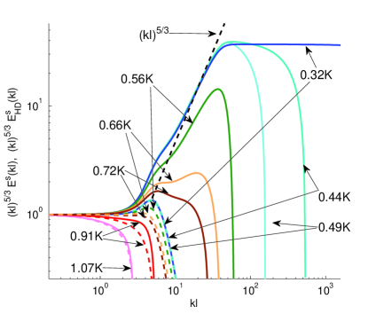
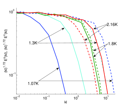
Figure 1: Color online. Log-Log plots of the energy spectra in superfluid ⁴He compensated by the inertial range scaling at different temperatures (shown as labels). Panel (a): Plots of the (compensated by $k^{5/3}$ and normalized by their values at $k\ell=0.1$) full superfluid energy spectra (solid lines) ${\mathcal{E}}^{\text{s}}(\kappa\ell)$ and their hydrodynamic (large scale) parts ${\mathcal{E}}^{\text{s}}_{\scriptscriptstyle\rm{HD}}(\kappa\ell)$ (dashed lines) for the one-fluid model (Sec. IV.2). Panel (b): Plots of the (compensated by the anomalous scaling $k^{1.72}$ and normalized by their inertial range value) shell energies of the normal fluid component $|u_{m}^{\text{n}}|^{2}=k{\mathcal{E}}^{\text{n}}(k_{m}\ell)$ (solid lines) and of the superfluid component $|u_{m}^{\text{s}}|^{2}=k{\mathcal{E}}^{\text{s}}(k_{m}\ell)$ (dashed lines) for the two-fluid shell model (Sec. III.2).

II.2.1 Low-temperature one-fluid energy spectra

First, we discuss the results for the eddy-wave model of superfluid turbulence [cf. Sec.  II.1.3], for the low temperature range $T\lesssim T_{\lambda}/2\simeq 1.08\,$K, which is shown in Fig. 1a. These spectra are compensated by a factor $(k\ell)^{5/3}$ such that both the Kolmogorov-Obukhov-41 spectrum ${\mathcal{E}}_{\scriptscriptstyle\rm{HD}}^{\text{s}}(k)\propto k^{-5/3}$, Eq. (6) (for the hydrodynamic scales $k\ell\ll 1$) and the Lvov-Nazarenko spectrum ${\mathcal{E}}_{\scriptscriptstyle\rm{KW}}^{\text{s}}(k)\propto k^{-5/3}$, Eqs. (5a) show up as a plateau. These plateaus are clearly seen for the lowest shown temperature $T=0.32\,$K. Moreover, the full energy spectrum (solid blue line) ${\mathcal{E}}^{\text{s}}(k)$ demonstrates the existence of an important bottleneck energy accumulation. We observe a large cross over region connecting the HD region $\kappa\ell<1$, where ${\mathcal{E}}^{\text{s}}(k)\to{\mathcal{E}}^{\text{s}}_{\scriptscriptstyle\rm{HD}}(k)$ with a much higher plateau ${\mathcal{E}}_{\scriptscriptstyle\rm{KW}}^{\text{s}}(k)$ for $k\ell>50$ where ${\mathcal{E}}^{\text{s}}(k)\to{\mathcal{E}}^{\text{s}}_{\scriptscriptstyle\rm{HD}}(k)$.

In the cross over region the compensated energy spectrum is close to $(k\ell)^{5/3}$ (cf. the black dashed line), meaning that ${\mathcal{E}}^{\text{s}}(k)$ depends on $k$ only weakly. In this region the energy spectrum is dominated by Kelvin waves, ${\mathcal{E}}^{\text{s}}(k)\simeq{\mathcal{E}}^{\text{s}}_{\scriptscriptstyle\rm{HD}}(k)$, while the energy flux in dominated by the HD eddy motions. Therefore we have here a flux-less regime of Kelvin waves. Without flux the situation resembles thermodynamic equilibrium, in which the Kelvin waves energy spectrum corresponds to energy equipartition between the degrees of freedom, i.e. $E^{\text{s}}_{\scriptscriptstyle\rm{KW}}(k)\sim$const, as observed.

For $k\ell>2\cdot 10^{4}$ the Kelvin waves energy spectrum at $T=0.32\,$K is suppressed by the mutual friction, as explained in Sec. IV.1. In Fig.1a this part of the spectrum is not shown; however one sees progressive suppression of the energy spectra with temperature increasing from 0.44 K (around $k\ell\simeq 400$) to $T=1.07\,$K (around $k\ell\simeq 2$). It is important to notice that for $T\geq 0.49\,$K the HD part of the spectrum is practically temperature independent; only the Kelvin waves energy spectra are suppressed by the temperature, cf. the coinciding dashed lines in Fig. 1a for $T=0.32\,,\ 0.44$ and 0.49  K.

For $T>0.5\,$K, the Kelvin wave contributions to the energy spectra are very small – the solid and the dashed lines for the same temperature are fairly close. Finally, the dashed and the solid lines for $T=1.07\,$K practically coincide, i.e. the Kelvin waves are fully damped. This means that for $T\gtrsim T_{\lambda}\sim 1\,$K there is no need to account for the Kelvin wave motions on individual vortex lines, and the full description of the problem is captured by the coarse-grained HVBK.

(a) Low $T\lesssim T_{\lambda}/2$, one-fluid model	(b) High $T\gtrsim T_{\lambda}/2$, two fluid model

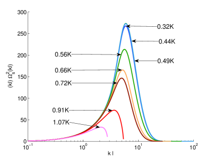
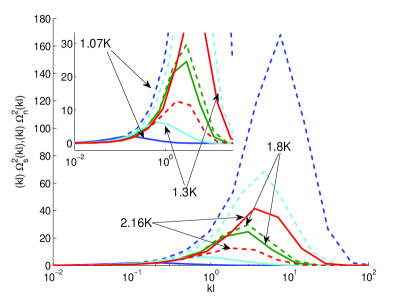
Figure 2: Color online. Color online. Linear-log plots of the vorticity spectral densities, $(k\ell)\,\Omega^{2}(k\ell)$, normalized by their $k\ell=0.1$ values, at different temperatures. The total mean-square vorticity $\left\langle\omega^{2}\right\rangle$ is proportional to the area under the plot. Panel (a): Superfluid vorticity spectra $(k\ell)\,\Omega_{\text{s}}^{2}(k\ell)$ at low temperatures in the one-fluid model, Sec. IV.2. Panel (b): Normal and superfluid vorticity spectra $(k\ell)\,\Omega_{\text{n}}^{2}(k\ell)$ (solid lines) and $(k\ell)\,\Omega_{\text{s}}^{2}(k\ell)$ (dashed lines) at high temperatures in the two-fluid model, Sec. III.2.

II.2.2 High-temperature two-fluid energy spectra

The energy spectra, obtained with the Sabra-shell model form of HVBK equations (2a) and (4), for temperatures $T\gtrsim T_{\lambda}/2\simeq 1.08\,$K, are shown Fig. 1b for $T=1.07\,$K (in blue), $T=1.3\,$K (in magenta), $1.8\,$K (in green) and $T=2.16\,$K (in red). The lowest temperature in this two-fluid approach, $T=1.07\,$K, was chosen for comparison with the highest temperature $1.07\,$K in the one-fluid approach; see Fig. 1a. At $T=1.3\,$K, which is a frequently used temperature in numerical simulations of superfluid turbulence, the normal fluid component is not negligible ($\rho_{\text{n}}/\rho\simeq 0.045$), and the normal fluid kinematic viscosity is still much larger than that of the superfluid: $\nu_{\text{n}}/\nu^{\prime}_{\text{s}}\simeq 23$. For $T=1.8$, when $\rho_{\text{n}}/\rho\simeq 0.3$, the kinematic viscosities are close to each other (see Tab. 1). At higher temperatures the normal fluid components play more and more important role until they dominate at $T>2.0\,$K, when $\rho_{\text{n}}>\rho_{\text{s}}$. At the highest temperature in this simulation, $T=2.16\,K$, close to $T_{\lambda}$, we have $\rho_{\text{n}}\approx 0.9\rho$, and the effective superfluid kinematic viscosity $\nu^{\prime}_{\text{s}}$ is even larger than $\nu_{\text{n}}$.

Shell-model simulations reproduce intermittency effects and therefore the scaling exponent $\xi_{2}$ of the energy spectra ${\mathcal{E}}(k)\propto k^{-\xi_{2}}$ slightly differs from the KO-41 prediction, $\xi_{2}\neq 5/3$. For the chosen shell-model parametersBLPP-2013 ; Sabra $\xi_{2}\approx 1.72$ which is quite close to the experimental observations. For better comparison with the low-temperature one-fluid results of Fig. 1a, we show in Fig. 1b the normal (solid lines) and superfluid (dashed lines) energy spectra ${\mathcal{E}}^{\text{n}}(k\ell)$ and ${\mathcal{E}}^{\text{s}}(k\ell)$, compensated by $(k\ell)^{1.72}$ so that they exhibit a plateau in the inertial interval of scales.

As expected, for $T=1.8\,$K, when $\nu_{\text{n}}\approx\nu_{\text{s}}^{\prime}$, the superfluid and normal fluid spectra are very close, and similar to the spectra of classical fluids. In the inertial range they demonstrate the anomalous behavior ${\mathcal{E}}^{\text{s}}\propto{\mathcal{E}}^{\text{n}}\propto k^{-\xi_{2}}$ $[|u_{m}^{\text{n}}|^{2}\propto k_{m}^{1-\xi_{2}}$] with the scaling exponent $\xi_{2}\approx 1.72$. Moreover, due to the strong coupling between the normal and superfluid component (discussed below in Sec. II.4) the energy fluxes in both components are equal (see, e.g. Fig. 4), and therefore the energies are equal in the inertial interval as well, ${\mathcal{E}}^{\text{s}}(k)={\mathcal{E}}^{\text{n}}(k)$. Non-trivial behavior occurs only in the inertial-viscous crossover region; therefore the inertial interval is not shown in Fig. 1.

For $T=1.07$, when $\nu_{\text{n}}\simeq 180\,\nu^{\prime}_{\text{s}}$, the viscous cutoff of the normal fluid’s spectrum, $k_{\text{max,n}}$, occurs at much smaller $k$ than the cutoff of the superfluid spectrum, $k_{\text{max,s}}$. To estimate the ratio $k_{\text{max,s}}/k_{\text{max,n}}$, notice that in the KO-41 picture of turbulence $k_{\text{max}}$ may be found by balancing the eddy-turnover frequency,

$$\gamma(k)\simeq\varepsilon^{1/3}k^{2/3}\simeq k^{3/2}\sqrt{{\mathcal{E}}(k)}\,,$$ (11)

with the viscous dissipation frequency $\nu k^{2}$. This gives the well known result

$$k_{\text{max}}\simeq\varepsilon^{1/4}/\nu^{3/4}\ .$$ (12)

In our case $\varepsilon_{\text{s}}=\varepsilon_{\text{n}}$. Therefore, neglecting the energy exchange between the super- and the normal-fluid components, we get an estimate:

$$\frac{k_{\text{max,s}}}{k_{\text{max,n}}}\simeq\Big{(}\frac{\nu_{\text{n}}}{\nu^{\prime}_{\text{s}}}\Big{)}^{3/4}\ .$$ (13)

For $T=1.07$, when $\nu_{\text{n}}\simeq 180\,\nu^{\prime}_{\text{s}}$ this gives $k_{\text{max,s}}/k_{\text{max,n}}\simeq 50$—in a good agreement with the result in Fig. 1b. For $T=1.3\,$K, the ratio of the viscosities is smaller (about $\simeq 23$, see Tab. 1). Therefore the difference in cutoffs is less pronounced. As expected, for $T=2.16\,$K, when $\nu_{\text{n}}\simeq 0.2\nu^{\prime}_{\text{s}}$ the situation is the opposite, and the superfluid component is damped at a smaller $k$ than the normal one.

Notice that there is no bottleneck energy accumulation in the spectra (see Figs. 1b) obtained using the shell model approximation of the gradually damped HVBK equations. This is qualitatively different from the results of the truncated HVBK model 22 , which demonstrated a very pronounced bottleneck both in the normal and the superfluid components, e.g. at $T=1.15\,$K. The latter would lead to a huge contribution to the mean square superfluid vorticity $\left\langle|\omega_{s}|^{2}\right\rangle$ and, as a result, to a very small effective Vinen’s viscosity $\nu^{\prime}_{\text{s}}$. This would definitely contradict the experimental observation shown in Fig. 5. We will discuss this issue in greater detail in Sec. II.5.

II.3 Temperature dependence of the vorticity spectra in turbulent ⁴He

At this point we cannot compare our predictions for energy spectra with experimental observations, especially in the cross-over and in the small scale regions. This stems from the lack of small probes, see cf. the review BLR . On the other hand, the attenuation of second sound or ion scattering may be used to measure the mean vortex line density ${\mathcal{L}}=1/\ell^{2}$ in ⁴He or even its time and space dependence BLR . In turn, the value ${\mathcal{L}}^{2}$ can be expressed in terms of the mean-square superfluid vorticity $\left\langle|\omega_{\text{s}}|^{2}\right\rangle$ via the quantum of circulation $\kappa$ Vin-2001 :

$$\left\langle|\omega_{\text{s}}|^{2}\right\rangle\approx(\kappa{\mathcal{L}})^{2}\ .$$ (14)

Therefore, the information about the vorticity is very important from the viewpoint of comparison with available and future experiments.

By analogy with the energy spectra (9), let us define the power spectra of vorticity $\Omega^{2}(k)$ so that the mean-square vorticity $\left\langle|\omega|^{2}\right\rangle$ is given by the integral:

$$\left\langle|\omega|^{2}\right\rangle=\int\limits_{0}^{\infty}\Omega^{2}(k)\,dk=\int\limits_{0}^{\infty}k\ \Omega^{2}(k)\,d\ln k\ .$$ (15)

In isotropic incompressible turbulence $\Omega^{2}(k)=2k^{2}{\mathcal{E}}_{\scriptscriptstyle\rm{HD}}(k)$. Therefore we define

$$\Omega^{2}_{\text{s}}(k)=2k^{2}{\mathcal{E}}^{\text{s}}_{\scriptscriptstyle\rm{HD}}(k)\,,\quad\Omega^{2}_{\text{n}}(k)=2k^{2}{\mathcal{E}}^{\text{n}}(k)\,.$$ (16)

For brevity, we omit the subscript “_HD” for the normal component; ${\mathcal{E}}^{\text{n}}_{\scriptscriptstyle\rm{HD}}(k)\Rightarrow{\mathcal{E}}^{\text{n}}(k)$.

Plots of $k\,\Omega^{2}_{\text{s,n}}(k)$ for different temperatures are shown in Figure 2. According to Eq. (15), the area under these plots is proportional to the total mean square vorticity, $\left\langle|\omega_{\text{s,n}}|^{2}\right\rangle$. Fig. 2a shows the results for the eddy-wave model (the corresponding energy spectra for the same temperatures are shown in Fig. 1a). One sees that the largest (and temperature independent) value of $\left\langle|\omega_{\text{s}}|^{2}\right\rangle$ is reached for $T<0.49\,$K: plots for $T=0.32\,\ 0.44\,$ and $0.49\,$K practically coincide. Accordingly, the temperature range $T<0.49\,$K may be considered as zero-temperature limit with the maximal value of $\left\langle|\omega_{\text{s}}|^{2}\right\rangle$ (and correspondingly, the smallest value of $\nu_{\text{s}}(T)$, as we will discuss later). At temperatures above 0.5K the area under the plots decreases (and correspondingly, $\nu_{\text{s}}(T)$ increases).

In Fig. 2b we show vorticity spectra $(k\ell)\left\langle|\omega_{\text{s,n}}|^{2}(k\ell)\right\rangle$ of the normal-fluid (solid lines) and the superfluid components (dashed lines) for different temperatures obtained in the framework of the Sabra-shell model (the corresponding spectra are shown in Fig. 1b). Again, the area under the plots is proportional to the total mean square vorticity $\left\langle|\omega_{\text{n,s}}|^{2}\right\rangle$. One sees that for the lowest temperature $T=1.07\,$K the normal fluid vorticity (blue solid line) is fully suppressed by the huge normal viscosity, while the superfluid vorticity is very large. At this temperature one can describe the superfluid ⁴He in the range of scales $k\ell\sim 1$ using a one-fluid approximation with zero normal-fluid velocity. This provides the main contribution to the vorticity. To some extent, this situation persists up to $T\approx 1.3\,$K, when the superfluid vorticity is still larger than the normal one, see Fig. 1b. As expected, for $T\simeq 1.8$, when the normal and superfluid viscosities are compatible, the normal and superfluid vorticities are very close. For these and higher temperatures the analysis of our problems definitely calls for a two-fluid description.

II.4 Correlations of normal and superfluid motions and energy exchange between components

High $T\gtrsim T_{\lambda}/2$, two-fluid model

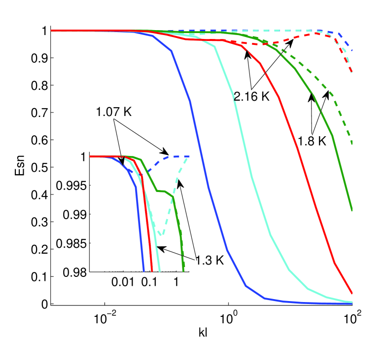
Figure 3: Color online. Cross-correlation coefficients $K_{1}(k\ell)$, Eq. (20a) (solid lines) and $K_{2}(k\ell)$ , Eq. (20b) (dashed lines) for different temperatures. Color code is the same as in Fig. 1b and Fig. 2b: $T=1.07\,$K – blue, $T=1.3\,$K – cyan, $T=1.8\,$K – green, and $T=2.16\,$K – red.

II.4.1 Correlations of the normal and superfluid velocities

It is often assumed (see e.g. Ref.VinenNiemela ) that the normal and superfluid velocities are “locked” in the sense that

$${\bm{u}}_{\text{n}}({\bm{r}},t)={\bm{u}}_{\text{s}}({\bm{r}},t)\,,$$ (17)

(at least in the inertial interval of scales). For quantitative understanding to which extent this assumption is statistically valid we consider the simplest possible case of stationary, isotropic and homogeneous turbulence. Here we introduce a cross-correlation function (in 1D $k$-representation) of the normal and the superfluid velocities ${\mathcal{E}}_{\text{ns}}(k)$. This correlation function is defined using the simultaneous, one-point cross-velocity correlation $\left\langle{\bm{u}}_{\text{n}}({\bm{r}},t)\cdot{\bm{u}}_{\text{s}}({\bm{r}},t)\right\rangle$ similarly to Eq. (9):

$$\int{\mathcal{E}}_{\text{ns}}(k)\,dk=\frac{1}{2}\left\langle{\bm{u}}_{\text{n}}({\bm{r}},t)\cdot{\bm{u}}_{\text{s}}({\bm{r}},t)\right\rangle\ .$$ (18)

If, for example, motions of the normal and the superfluid components at a given $k$ are completely correlated, then ${\mathcal{E}}_{\text{ns}}(k)={\mathcal{E}}_{\text{n}}(k)={\mathcal{E}}_{\text{s}}(k)$. If this is true for all scales, then Eq. (17) is valid.

It is natural to normalize ${\mathcal{E}}_{\text{ns}}$ by the normal and the superfluid energy densities, ${\mathcal{E}}_{\text{n}}$ and ${\mathcal{E}}_{\text{s}}$. This can be reasonably done in one of two ways:

$${\mathcal{K}}_{1}(k)\equiv\frac{2\,{\mathcal{E}}_{\text{ns}}(k)}{{\mathcal{E}}_{\text{n}}(k)+{\mathcal{E}}_{\text{ s}}(k)}\,,$$ (19a)

$$\hbox{or}\;\;\;{\mathcal{K}}_{2}(k)\equiv\frac{{\mathcal{E}}_{\text{ns}}(k)}{\sqrt{{\mathcal{E}}_{\text{n}}(k)\cdot{\mathcal{E}}_{\text{ s}}(k)}}\ .$$ (19b)

Both coefficients are equal to unity for fully locked superfluid and normal velocities, Eq. (17), and both vanish if the velocities are statistically independent. However, if ${\bm{u}}_{\text{n}}({\bm{r}},t)=C{\bm{u}}_{\text{s}}({\bm{r}},t)$, with $C\neq 1$ then ${\mathcal{K}}_{1}(k)=2C/(C^{2}+1)<1$, but still ${\mathcal{K}}_{2}(k)=1$. In any case ${\mathcal{K}}_{1}(k)\leqslant{\mathcal{K}}_{2}(k)$.

In shell models, the coefficients ${\mathcal{K}}_{1}(k)$ and ${\mathcal{K}}_{2}(k)$ can be written as follows:

$$K_{1}(k_{m}\ell) \equiv \frac{2\,\mbox{Re}\left\langle v_{m}^{\text{s*}}v_{m}^{\text{n}}\right\rangle}{\left\langle v_{m}^{\text{s*}}v_{m}^{\text{s}}\right\rangle+\left\langle v_{m}^{\text{n*}}v_{m}^{\text{n}}\right\rangle}\,,$$ (20a)

$$K_{2}(k_{m}\ell) \equiv \frac{\mbox{Re}\left\langle v_{m}^{\text{s*}}v_{m}^{\text{n}}\right\rangle}{\sqrt{\left\langle(v_{m}^{\text{s*}}v_{m}^{\text{s}}\right\rangle\left\langle v_{m}^{\text{n*}}v_{m}^{\text{n}}\right\rangle}}\ .$$ (20b)

These objects are shown in Fig. 3. At first glance, it is surprising that the correlations $K_{2}(k_{m}\ell)$ (dashed lines in Fig. 3) for $T\lessgtr 1.8\,$K persist for much larger wave vectors than $K_{1}(k_{m}\ell)$, approaching $k_{m}\ell\sim 10^{2}$. For example, for $T=1.07\,$K (blue lines) $K_{1}(k_{m}\ell)$ vanishes at $k_{m}\ell\simeq 1$, while $K_{2}(k_{m}\ell)>0.95$ all the way up to $k_{m}\ell\simeq 100$. In this range of scales ($1\lesssim k_{m}\ell\lesssim 100$) $v_{m}^{\text{n}}\ll v_{m}^{\text{s}}$, but $v_{m}^{\text{n}}(t)\propto v_{m}^{\text{s}}(t)$, meaning that strongly damped normal velocity does not have its own dynamics and should be considered as “slaved” by the superfluid velocity. The damped velocity (normal or superfluid) at any temperature $T\lessgtr 1.8\,$K would follow this ”slaved” dynamics.

A model expression of the cross-correlation ${\mathcal{E}}_{\text{sn}}$ in terms of the self-correlation functions ${\mathcal{E}}_{\text{s}}$ and ${\mathcal{E}}_{\text{n}}$ was found in LABEL:L199. In current notations it reads:

$${\mathcal{E}}_{\text{sn}}(k)=\frac{\alpha\,\bar{\omega}_{\text{s}}[\rho_{\text{n}}\,{\mathcal{E}}_{\text{n}}(k)+\rho_{\text{s}}\,{\mathcal{E}}_{\text{s}}(k)]}{\alpha\,\bar{\omega}_{\text{s}}\rho+\rho_{\text{n}}[(\nu^{\prime}_{\text{s}}+\nu_{\text{n}})\,k^{2}+\gamma_{\text{n}}(k)+\gamma_{\text{s}}(k)]}\,,$$ (21)

where the characteristic interaction frequencies (or turnover frequencies) of eddies in the normal and superfluid components, $\gamma_{\text{n}}(k)$ and $\gamma_{\text{s}}(k)$, are given by Eq. (11) and $\bar{\omega}_{\text{s}}$ is defined as:

$$\bar{\omega}_{\text{s}}\equiv\sqrt{\left\langle|\omega_{\text{s}}|^{2}\right\rangle}\ .$$ (22)

The derivation of Eq. (21) in LABEL:L199 involves diagrammatic perturbation approach and is rather cumbersome. However the simplicity of the final result (21) motivated us to re-derive it in a simple and transparent way which is presented in the Appendix.

Let us analyze first Eq. (21) in the inertial interval of scales, where according to Fig. 1b, ${\mathcal{E}}_{\text{s}}={\mathcal{E}}_{\text{n}}$ and the terms with the viscosities in the denominator may be neglected. In this case

$${\mathcal{K}}_{1}(k) \to \Big{[}1+\frac{2\rho_{\text{n}}\gamma_{\text{s}}(k)}{\alpha\,\rho\,\bar{\omega}_{\text{s}}})\Big{]}^{-1}$$

$$\simeq \Big{[}1+\frac{2\,\rho_{\text{n}}}{\alpha\,\rho}\Big{(}\frac{k}{k_{\text{max,s}}}\Big{)}^{2/3}\Big{]}^{-1}\,,$$

where the viscous cutoff of the superfluid inertial interval $k_{\text{max,s}}$ is given by estimate (12). First of all we see that the correlation coefficient is governed by the dimensionless parameter $\alpha\rho/\rho_{\text{n}}$ which involves the mutual friction coefficient $\alpha$, as expected. What is less expected, is that this parameter, according to Tab. 1, depends on the temperature only weakly and is close to unity. Therefore, in the inertial interval $k\ll k_{\text{max,s}}$ we have:

$${\mathcal{K}}_{1}(k) \simeq \Big{[}1+\frac{2\,\rho_{\text{n}}}{\alpha\,\rho}\Big{(}\frac{k}{k_{\text{max,s}}}\Big{)}^{2/3}\Big{]}^{-1}$$

$$\simeq 1-\Big{(}\frac{k}{k_{\text{max,s}}}\Big{)}^{2/3}\,,$$

and this expression is very close to unity. In the other words, in the inertial interval we expect the full locking of the normal and the superfluid velocities for all temperatures. This prediction fully agrees with the observations in Fig. 3.

Consider now case $T=1.07\,$K, when $k_{\text{max,s}}\simeq 50\,k_{\text{max,n}}$ according to the data in Fig. 1b and estimate (13). For $k_{\text{max,n}}<k<k_{\text{max,s}}$ we have:

$$\ {\mathcal{E}}_{\text{s}}(k)\gg{\mathcal{E}}_{\text{n}}(k)\,,\ \ \mbox{and}\ \ \nu_{\text{n}}\gg\gamma_{\text{s}}(k)\gg\gamma_{\text{n}}(k)\gg\nu^{\prime}_{\text{s}}\ .$$ (25)

Then Eq. (21) simplifies to the following form,

$${\mathcal{K}}_{1}(k)\simeq\Big{[}1+\frac{\rho_{\text{n}}}{\alpha\,\rho}\frac{\nu_{\text{n}}k^{2}}{\bar{\omega}_{\text{s}}}\Big{]}^{-1},$$

and it may be analyzed as follows:

$${\mathcal{K}}_{1}(k)\simeq\Big{[}1+\frac{\rho_{\text{n}}}{\alpha\,\rho}\frac{\nu_{\text{n}}k^{2}}{\bar{\omega}_{\text{s}}}\Big{]}^{-1}\simeq\Big{[}1+\frac{\nu_{\text{n}}k^{2}}{\nu^{\prime}_{\text{s}}\,k^{2}_{\text{max,s}}}\Big{]}^{-1}$$

Using (13), for $\ k\sim k_{\text{max,s}}$ we get

$${\mathcal{K}}_{1}(k)\simeq\Big{[}1+\frac{k^{4/3}_{\text{max,s}}}{k^{4/3}_{\text{max,n}}}\Big{]}^{-1}\sim\frac{k^{4/3}_{\text{max,n}}}{k^{4/3}_{\text{max,s}}}\ll 1\,,$$ (26)

We see that the velocities decorrelate in the interval $k_{\text{max,n}}<k<k_{\text{max,s}}$, as expected.

Estimating ${\mathcal{K}}_{2}(k)$ in the regime (25) is less simple, because it requires knowledge of the ratio ${\mathcal{E}}_{\text{s}}(k)/{\mathcal{E}}_{\text{n}}(k)$ in terms of $\nu_{\text{n}},\nu^{\prime}_{\text{s}},\gamma_{n}(k)$ and $\gamma_{s}(k)$. Instead, we can directly use Eq. (61b), which in regime  (25) may be simplified (in the $({\bm{k}},t)$-representation) as follows:

$$u_{\text{n}}({\bm{k}},t)=\frac{\alpha\,\rho_{\text{s}}\,\bar{\omega}_{\text{s}}}{\rho_{\text{n}}\nu_{\text{n}}k^{2}}\,u_{\text{s}}({\bm{k}},t)\ll u_{\text{s}}({\bm{k}},t)\ .$$ (27)

i.e. $u_{\text{n}}({\bm{k}},t)$ is slaved by $u_{\text{s}}({\bm{k}},t)$. Equation (27) immediately gives ${\mathcal{K}}_{1}(k)\ll 1$, but ${\mathcal{K}}_{2}(k)=1$ in full agreement with our results in Fig. 3. In particular, this means that our simple model of correlations between ${\bm{u}}_{\text{n}}$ and ${\bm{u}}_{\text{s}}$, suggested in the Appendix, quantitatively correctly reflects the basic physics of this phenomenon.

High $T\gtrsim T_{\lambda}/2$, two fluid model

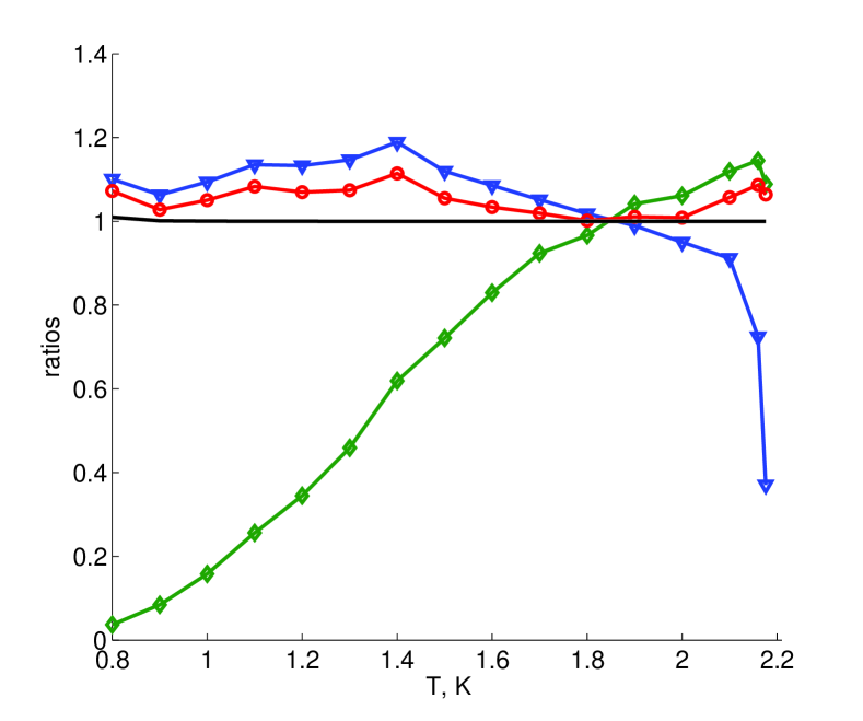
Figure 4: Color online. Temperature dependence of the ratios: $\varepsilon_{\text{s}}/\varepsilon_{\text{n}}$ – horizontal black line; $R_{\text{s}}$, Eq. (28a), – blue line with triangles, $R_{\text{n}}$, Eq. (28a), – green line with diamonds, $R_{\text{s+n}}$, Eq. (28b), – red line with circles.

II.4.2 Energy dissipation and exchange due to mutual friction

Strong coupling of the normal and the superfluid velocities suppresses the energy dissipation and the energy exchange between the normal and the superfluid components caused by the mutual friction (which is proportional to ${\bm{u}}_{\text{s}}-{\bm{u}}_{\text{n}}$, Eq. (1c)). Nevertheless, some dissipation due to the mutual friction is still there. Consider the ratio of the total injected energy to the total energy dissipated due to the viscosity in the normal and the superfluid components:

$$R_{\text{s+n}}=\frac{\rho_{\text{s}}\varepsilon_{\text{s}}+\rho_{\text{n}}\varepsilon_{\text{n}}}{\rho_{\text{s}}\nu^{\prime}_{\text{s}}\left\langle|\omega_{\text{s}}|^{2}\right\rangle+\rho_{\text{n}}\nu_{\text{n}}\left\langle|\omega_{\text{n}}|^{2}\right\rangle}\ ,$$ (28a)

a quantity plotted in Fig. 4 (red line with circles). Here $$\varepsilon_{\text{n}} \varepsilon_{\text{s}} \sim 10\% T\approx 1.8\, {\bm{u}}_{\text{s}}\approx{\bm{u}}_{\text{n}}$$ and are the inertial range normal and superfluid energy fluxes. This ratio exceeds unity by about 10%, meaning that of the injected energy is dissipated by the mutual friction. As expected, this effect disappears at K, when the effective superfluid and normal fluid kinematic viscosities are matching (and therefore ).

The mutual friction has a significantly more important influence on the energy exchange between the normal and the superfluid components. The energy exchange can be quantified by a similar ratio defined for each fluid component,

$$R_{\text{s}}=\frac{\varepsilon_{\text{s}}}{\nu^{\prime}_{\text{s}}\left\langle|\omega_{\text{s}}|^{2}\right\rangle}\,,\quad R_{\text{n}}=\frac{\varepsilon_{\text{n}}}{\nu_{\text{n}}\left\langle|\omega_{\text{n}}|^{2}\right\rangle}\,,$$ (28b)

shown by a green line with diamonds and a blue line with triangles respectively in Fig. 4. At the lowest shown temperature $T=0.8\,$K, we have $R_{\text{n}}<0.1$ meaning that only about 10% of the energy density (per unit mass) which is dissipated by the normal fluid component comes from the direct energy input. The rest $\simeq 90\%$ of the energy density dissipated by viscosity (at large $k$) was transferred from the superfluid component by the mutual friction. This is because for $T\lesssim 1.8\,$K, we have $\nu_{\text{n}}>\nu^{\prime}_{\text{s}}$ and therefore the normal velocity becomes more damped at lower wavenumbers than the superfluid velocity, see Fig. 1b. Such an energy transfer by mutual friction from the superfluid component to the normal one increases $R_{\text{s}}$ (blue line with triangles) above unity. This effect is smaller than the one for $R_{\text{n}}$ because at low temperatures $\rho_{\text{s}}\gg\rho_{\text{n}}$ and the energy per unity volume $\rho_{\text{s}}\varepsilon_{\text{s}}+\rho_{\text{n}}\varepsilon_{\text{n}}$ is approximately conserved. As expected, there is no energy exchange between the components at $T\approx 1.8\,$K, when $\nu_{\text{n}}=\nu^{\prime}_{\text{s}}$ and ${\bm{u}}_{\text{s}}={\bm{u}}_{\text{n}}$). At this temperature $R_{\text{s}}=R_{\text{n}}=R_{\text{n+s}}=1$. Again, as expected for $T>1.8\,$K, when $\nu_{\text{n}}<\nu^{\prime}_{\text{s}}$ (see Tab. 1) we have $R_{\text{s}}>1$, $R_{\text{n}}<1$ meaning that the energy goes from the less damped normal component to the more damped superfluid one.

To understand why the energy exchange due to the mutual friction is larger than the energy dissipation by the mutual friction, notice that the energy exchange is proportional to the (small) velocity difference, $\left\langle{\bm{u}}_{\text{n}}\cdot({\bm{u}}_{\text{n}}-{\bm{u}}_{s})\right\rangle$, while the energy dissipation is proportional to the square of this parameter, $\left\langle|{\bm{u}}_{\text{n}}-{\bm{u}}_{\text{s}}|^{2}\right\rangle$.

Low $T\lesssim T_{\lambda}/2$, one-fluid model

High $T\gtrsim T_{\lambda}/2$, two-fluid model

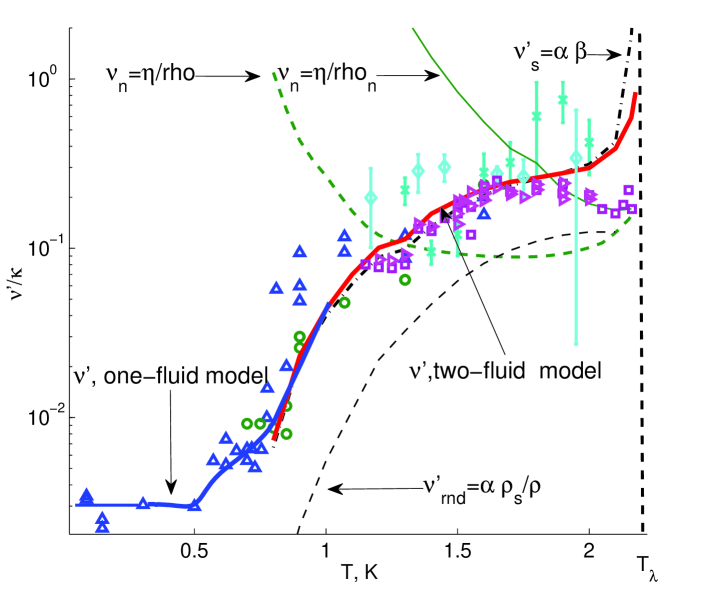
Figure 5: Color online. Comparison of the experimental, numerical and analytical results for the temperature dependence of the effective kinematic viscosities: Blue triangles – Manchester spin-down experiments Manchester-exp ; Green empty circles – Manchester ion-jet experiments Golov2 ; sea-green diamonds with error-bars – Prague counterflow experiments Ladik ; cian crosses with error-bars – Prague decay in grid co-flow experiments Ladik1 ; Magenta empty squares – Oregon towed grid experiments stalp ;Pink right triangles–Oregon towered grid experiments nimiela2005 . Solid green line – experimental results DonnelyBarenghi98 for the normal-fluid kinematic viscosity $\nu_{\text{n}}=\mu/\rho_{\text{n}}$ (normalized by the normal-fluid density); Dashed green line – He-II kinematic viscosity $\nu\equiv\mu/\rho$, (normalized by the total density) – see also Tab. 1. Thin black dash line – effective viscosity for the random vortex tangle $\nu^{\prime}_{\text{rnd}}$, estimated by Eq. (31); Thick dot-dashed black line – the Vinen-Niemela estimate VinenNiemela of the effective superfluid viscosity, $\nu^{\prime}_{\text{s}}$, given by Eq. (32). Blue solid line – $\nu^{\prime}(T)$ at $T<1.1\,$K from numerical solution of Eqs. (51c) for the one-fluid differential model of gradual eddy-wave crossover; Red solid line – $\nu^{\prime}(T)$ at $T>0.9\,$K from numerical simulations in Sec. III.2 of gradually damped two-fluid HVBK Eqs. (1) in the Sabra shell-model approximation (33).

II.5 Temperature dependence of the effective superfluid viscosity in ⁴He

The temperature-dependent effective (Vinen’s) viscosity $\nu^{\prime}(T)$ is defined stalp by the relation between the rate of energy-density (per unit mass) flux into turbulent superfluid, $\varepsilon$, and the vortex-line density, ${\mathcal{L}}$:

$$\varepsilon=\nu^{\prime}(T)(\kappa{\mathcal{L}})^{2}\approx\nu^{\prime}(T)\left\langle|\omega_{\text{s}}|^{2}\right\rangle\ .$$ (29)

According to Eq. (15), $\left\langle|\omega_{\text{s}}|^{2}\right\rangle$ is proportional to the area under the plots $k\,\Omega^{2}_{\text{s}}(k)$ vs. $\log k$, shown in Fig. 2 and discussed in Sec. II.3. These results allow us to determine the viscosity $\nu^{\prime}(T)$ (analytically and numerically) in the entire temperature range from $T\to 0$ up to $T\to T_{\lambda}$.

II.5.1 Low temperature range $T\lesssim T_{\lambda}/2$

Consider first the temperature dependence of $\nu^{\prime}(T)$ in the low temperature range $T\lesssim T_{\lambda}/2\approx 1.1\,$K, shown in Fig. 5 by the solid blue line. This dependence is found in Sec. IV.2 in the framework of one-fluid model of gradual eddy-wave crossover Eqs. (51). As we mentioned, the largest (and temperature independent) value of $\left\langle|\omega_{\text{s}}|^{2}\right\rangle$ (at fixed value of $\varepsilon_{\text{s}}$) is reached for $T<0.49\,$K. Accordingly, the temperature range $T<0.49\,$K may be considered as a zero-temperature limit, at which $\nu^{\prime}(T)$ reaches its smallest value. The results of the Manchester spin-down experiment Manchester-exp are temperature independent as well (within the natural scatter of the data). The particular value of $\nu^{\prime}_{\text{exp}}(T\to 0)\simeq 0.003\,\kappa$ found in these experiments is probably accurate up to a numerical factor ${(\frac{1}{3}\div 3)}$ due to uncertainty in the determination of the outer scale of turbulence, taken in Ref. Manchester-exp for simplicity as the size of the cube. Our low-temperature, one-fluid model (51) involves one fitting parameter, which determines the crossover scale in the blending function Eq.(48). This parameter affects the resulting value of $\nu^{\prime}_{\text{mod}}(T\to 0)$ and was chosen such as to meet its accepted experimental value $\nu^{\prime}_{\text{exp}}(T\to 0)\simeq 0.003\,\kappa$.

At temperatures above 0.5 K, the area under the $k\Omega^{2}_{\text{s}}(k)$ plots in Fig. 2a become smaller and smaller. This is caused by the suppression of the Kelvin wave spectra, which is more pronounced at larger temperature, as seen in Fig. 1a. The value of $\left\langle|\omega_{\text{s}}|^{2}\right\rangle$ decreases with the temperature resulting in a progressive increase in $\nu^{\prime}(T)$ as shown by the solid blue line in Fig. 5 together with the experimental (Manchester spin-downManchester-exp and ion-jetGolov2 ) values of $\nu^{\prime}_{\text{exp}}(T)$. There is a reasonably good agreement between the temperature dependence of $\nu^{\prime}(T)$ found in the framework of the one-fluid model of eddy-wave crossover at low temperatures and the experiments. Importantly, in the modeling we have used only one phenomenological parameter to fit the zero-$T$ limit of $\nu^{\prime}_{\text{exp}}(T)$, while the temperature dependence of the latter follows from the model without any additional fitting.

II.5.2 High temperature range $T\gtrsim T_{\lambda}/2$

At $T\gtrsim 1\,$K, Kelvin waves are already fully damped; see Fig. 1a. This means that for these temperatures we can use the coarse-grained HVBK Eqs. (1). Using the shell model approximation we find the temperature dependence of $\nu_{\text{s}}(T)$ in the temperature range $T>0.8\,$K as shown in Fig. 5 by the solid red line. In the intermediate temperature range $0.9\,$K$<T<1.1\,$K this line overlaps with the blue solid line, showing the one-fluid results. The reason for this overlap is very simple: for $0.9\,$K$<T<1.1\,$K, the Kelvin waves are already damped (see Fig. 1a), and the normal-fluid eddies at scales $k\ell\sim 1$ are still damped. Therefore, in this range both the one-fluid model and the coarse-grained model describe the physics equally well. Moreover, the effective viscosity $\nu^{\prime}$ in the one-fluid approximation, suggested in Ref.VinenNiemela and shown as the black dot-dashed line in Fig. 5, gives the same result as the two our approaches. At $T<0.9\,$K the coarse-grained (blue and black) results deviate below the one-fluid prediction which also accounts for the energy transfer to the Kelvin waves. This results in a slower decrease of $\nu^{\prime}(T)$ with temperature, and finally, in the zero temperature limit (i.e. below $0.5\,$K) this predicts the plateau which is fully determined by the bottleneck energy accumulation at the crossover between the hydrodynamic and the Kelvin wave regimes of the superfluid motions.

For temperatures above $1.1\,$K, the normal fluid contribution to the two-fluid dynamics becomes important, and the two-fluid results in Fig. 5 (red solid line) deviate above the value of $\nu^{\prime}_{\text{s}}(T)$ which is determined by the superfluid component alone, cf. Ref.VinenNiemela . This is because in this temperature interval the normal-fluid viscosity $\nu_{\text{n}}(T)$ (dashed green line) is much higher than its superfluid counterpart $\nu^{\prime}_{\text{s}}$. Therefore there exists an energy flux which is induced by the mutual friction from the less damped superfluid component to the normal fluid component. This is seen in Fig. 4, were $R_{\text{s}}>1$ and $R_{\text{n}}<1$. Thus $\left\langle|\omega_{\text{s}}|^{2}\right\rangle$ is suppressed and correspondingly $\nu^{\prime}(T)$ deviates above $\nu^{\prime}_{\text{s}}$ (the black dot-dashed line) that does not account for the energy exchange. Clearly, at $T\simeq 1.8\,$K , when there is no energy exchange, $\nu^{\prime}(T)$ should be equal to $\nu^{\prime}_{\text{s}}$. Also it is clear that for $T\gtrsim 1.8\,$K, when the energy flows in the opposite direction (from the normal- to the super-fluid component), one expects that $\nu^{\prime}(T)$ should be smaller than $\nu^{\prime}_{\text{s}}$. All these expectations are confirmed by the results shown in Fig. 5.

In Fig. 5 we also show the results for $\nu^{\prime}(T)$ of the Prague counterflow Ladik and co-flow decay Ladik1 experiments and those of the Oregon towered gridstalp ; nimiela2005 experiments. These high-$T$ experimental data have a significant scatter for reasons discussed in Refs. Ladik ; Ladik1 ; Ladik2 .

Taking into account the scatter of the experimental data, our computed dependence of $\nu^{\prime}(T)$ agrees reasonably well with experiments in various flows in the entire range of temperatures from $T\to 0$ up to $T\to T_{\lambda}$.

III Coarse-grained, two-fluid dynamics of superfluid turbulence

This Section concentrates on the high-temperature regime, say $T\gtrsim T_{\lambda}/2$, when the small-scale motions (Kelvin waves) are effectively damped and we can restrict ourselves to a coarse-grained description of the superfluid dynamics in the continuous-media approximation. In most of this temperature range both the normal and the superfluid components play important role and the two-fluid description is required.

III.1 Coarse-grained, two-fluid, gradually-damped HVBK equations

In this subsection we discuss in more details the gradually-damped HVBK model, presented by Eqs. (1).

III.1.1 Simple closure for the large-scale energy dissipation due to mutual friction

Originally in HVBK equations the mutual friction force has the form:

$${\bm{F}}_{\text{ns}}=\alpha~{}\hat{{\bm{\omega}}}_{\text{s}}\times[{\bm{\omega}}_{\text{s}}\times({\bm{u}}_{\text{n}}-{\bm{u}}_{\text{s}})]+\alpha^{\prime}{\bm{\omega}}_{\text{s}}\times({{\bm{u}}_{\text{s}}}-{\bm{u}}_{\text{n}})\ .$$ (30)

Here ${\bm{\omega}}_{\text{s}}\equiv\nabla\times{\bm{u}}_{\text{s}}$ is the superfluid vorticity and the unit vector $\hat{{\bm{\omega}}}_{\text{s}}\equiv{\bm{\omega}}_{\text{s}}/\omega_{\text{s}}$ is pointing in the direction of the vorticity. The dimensionless phenomenological parameters $\alpha$ and $\alpha^{\prime}$ describe the dissipative and the reactive mutual friction forces acting on a vortex line as it moves with respect to the normal component.

In our Eqs. (1) we used the simplified form (1c) of the mutual friction which accounts for the fact that the vorticity in developed turbulence is usually dominated by the smallest eddies in the system, with the Kolmogorov viscous scale $\eta$ and with the largest characteristic wave-vector $k_{\eta}\sim 1/\eta$. These eddies have the smallest turnover time $\tau_{\eta}$ which is of the order of their decorrelation time. On the contrary, the main contribution to the velocity in the equation for the dissipation of the $k$-eddies with intermediate wave-vectors $k$, $k\ll k_{\eta}$, is dominated by the $k^{\prime}$-eddies with $k^{\prime}\sim k$. Because the turnover time of these eddies $\tau_{k^{\prime}}\gg\tau_{\eta}$, we can justify the approximation (1c) by averaging the vorticiy in Eqs. (30) during the time intervals of interest ($\tau_{\eta}\ll\tau\ll\tau_{k^{\prime}}$). Thus the vorticity ${\bm{\omega}}_{\text{s}}$ may be considered as uncorrelated with the velocities ${\bm{u}}_{\text{s}},{\bm{u}}_{\text{n}}$, which are the dynamical variables. More detailed analysis Lvov shows that the approximation (1c) directly follows from the Kraichnan’s Direct Interaction Approximation in the Belinicher-Lvov sweeping-free representation for the velocity triple-correlations.

III.1.2 Vinen-Niemela model for the superfluid energy dissipation

The energy dissipation term involving $\nu^{\prime}_{\text{s}}$ in Eq. (1a) for the superfluid velocity attempts to take into account the existence of quantized vortex lines in an essentially classical regime of motion. An early approach to this dissipation term nueff was based on a picture of a random vortex tangle moving in a quiescent normal component. With the definition (29) this picture leads to the simple equations for the effective viscosity Ladik2 :

$$\nu^{\prime}_{\text{rnd}}=\alpha\rho_{\text{s}}\big{/}\rho\,,$$ (31)

shown by a black thin dashed line in Fig. 5. One sees that this result is much lower than the experimental data. Moreover, the picture of a random vortex tangle moving in a quiescent normal fluids predicts a higher dissipation compared to the realistic situation in which the normal and superfluid velocities are almost locked together as discussed in Sec. II.4. The missing physics that needs to be considered to resolve this contradiction is that of vortex reconnections.

During reconnections, sharp angles necessarily appear on the vortex lines, leading to their fast motion. This motion is uncorrelated with the motion of other vortex lines (except the ones involved in the reconnection) as well as with the (relatively slow) motion of the normal-fluid component. This leads to large local energy dissipation events due to the mutual friction, which smoothes the vortex lines and removes the regions of high curvature appearing after the reconnection events. A detailed analysis of this and related effects led Vinen and Niemela VinenNiemela to suggest the effective superfluid (kinematic) viscosity $\nu^{\prime}_{\text{s}}$ which in our notations reads:

$$\nu^{\prime}_{\text{s}}=\beta(T)\,\alpha\kappa\,,\qquad\beta(T)\equiv s\,\Big{(}\frac{c_{2}\Lambda}{4\pi}\Big{)}^{2}\ .$$ (32)

Here, the parameter $c_{2}$ relates the vortex line density and the mean-square curvature26 ; KLPP-2014 , and the parameter $s<1$ accounts for the suppression of effective line density due to partial polarization of vortex lines and was roughly estimated in Ref.VinenNiemela as 0.6. The temperature dependence of $\nu^{\prime}_{\text{s}}(T)$ estimated with the help of Tab. III of LABEL:VinenNiemela is presented in Tab. 1. The resulting plot of $\nu^{\prime}_{\text{s}}(T)$ is shown in Fig. 5 by a thick black dot-dashed line. Besides the clear and definitely relevant physics underlying Eq. (32), it agrees well with the experiments. That is why in our analysis we will include effective damping (32) in our gradually damped HVBK model Eq. (1a).

III.1.3 Truncated vs. gradually-damped HVBK models

A previous model which is referred to as the “truncated HVBK model” of superfluid turbulence was suggested in LABEL:22. The idea was to account for the strong suppression of Kelvin waves at high temperatures by simply truncating the HVBK equation for the superfluid at a cutoff wavenumber $k_{\ell}=\tilde{\beta}/\ell$ (at which the normal fluid is expected to be well damped by the viscosity), using a fitting parameter $\tilde{\beta}$ of the order of unity. An obvious limitation of this model is the abruptness of the truncation. An attempt to use this model for the calculation of the effective viscosity Ladik2 shows that the resulting $\nu^{\prime}$ [denoted in  Ref.Ladik2 as $\nu_{\text{eff}}$] may vary by a factor of about five, when $\widetilde{\beta}$ changes by the same factor (see Fig. 4, Top, in  Ref.Ladik2 ). Moreover, due to the strong temperature dependence of the normal-fluid viscosity $\nu_{\text{n}}$, the truncation scale depends strongly on temperature, as illustrated in our Fig. 1b. This means that the fitting parameter $\tilde{\beta}$ should be temperature dependent. If so, the truncated HVBK model looses its predictive power. We remark however that the experimental values of the effective viscosity presented in  Ref.Ladik2 unaffected by issues with the truncated HVBK equations discussed here.

Unfortunately, this is not the only problem in the analysis of $\nu_{\text{eff}}$ in LABEL:Ladik2. For interpreting the results of the numerical simulations of the truncated HVBK model the authors of LABEL:Ladik2 use Eq. (31) for $\nu^{\prime}_{\text{rnd}}$ which presumes the random vortex tangle. The values of $\nu^{\prime}_{\text{rnd}}$ are shown in Fig. 5 by a black thin dashed line. As we already noticed in Sec. III.1.2 these values are smaller by one order of magnitude as compared to the experimental points. The physical reason for this discrepancy is very simple. The truncated HVBK model ignores the energy dissipation in the reconnection events, that, according to our simulations of gradually-damped HVBK model illustrated in Fig. 4, constitute more than $90\%$ of the total energy dissipation in the system.

III.2 Two-fluid Sabra shell-model of turbulent ⁴He

III.2.1 Sabra-shell model equations

Following s5 we can present gradually damped HVBK Eqs. (1) for isotropic space-homogeneous turbulence as the system of two shell model equations for the normal $v^{\text{n}}_{\text{m}}$ and superfluid $v^{\text{s}}_{\text{m}}$ shell velocities coupled by the friction force term. In the dimensionless form it may be written as follows:

$$\Big{[}\frac{d}{d\tau}+\widetilde{\nu}_{\text{n}}\,k_{m}^{2}\Big{]}v^{\text{n}}_{m} = \mbox{NL}_{m}\{v^{\text{n}}_{m^{\prime}}\}+\frac{\rho_{\text{s}}}{\rho_{n}}F_{m}+f_{m}^{\text{n}}\,,$$ (33a)

$$\Big{[}\frac{d}{d\tau}+\widetilde{\nu}_{\text{s}}^{\prime}\,k_{m}^{2}\Big{]}v^{\text{s}}_{m} = \mbox{NL}_{m}\{v^{\text{s}}_{m^{\prime}}\}-F_{m}+f_{m}^{\text{s}}\,,$$ (33b)

$$\widetilde{\nu}_{\text{n}}=\frac{\nu_{\text{n}}}{\kappa\,\mbox{Re}_{\kappa}}\,, \widetilde{\nu}_{\text{s}}^{\prime}=\frac{\nu_{\text{s}}^{\prime}}{\kappa\,\mbox{Re}_{\kappa}}\,,$$ (33c)

$$\mbox{Re}_{\kappa}=\frac{L\,U_{\scriptscriptstyle\rm{T}}}{\kappa}\,, U_{\scriptscriptstyle\rm{T}}^{2}=2\frac{\big{[}\rho_{\text{s}}K_{\text{s}}+\rho_{\text{n}}K_{\text{n}}\big{]}}{\rho}\,,$$

$$K_{\text{s}}=\frac{1}{2}\sum_{m}|v_{m}^{\text{s}}|^{2}\,, \quad K_{\text{n}}=\frac{1}{2}\sum_{m}|v_{m}^{\text{n}}|^{2}\,,$$ (33d)

$$F_{m}=\alpha\,\omega_{\text{s}}(v^{\text{s}}_{m}-v^{\text{n}}_{m})\,,\hskip-28.45274pt \qquad\omega_{\text{s,n}}^{2}\equiv\sum_{m}k_{m}^{2}|v_{m}^{\text{s,n}}|^{2}.$$ (33e)

Here NL${}_{m}\{v_{m^{\prime}}\}$ is the Sabra nonlinear term, given by Eq. (4). The dimensionless shell wave numbers $k_{m}$ are chosen as a geometric progression $k_{m}=k_{0}2^{m}$, where $m=1,2,\dots\,M$ are the shell indices, and the dimensionless reference shell wave number is normalized by the inverse outer scale of turbulence $1/L$ (to be specific, in our simulations we have chosen $k_{0}=1/16$).

The NL${}_{m}\{v_{m^{\prime}}\}$ term (4) conserves the kinetic energy (per unite mass) $K_{\text{s}}$ and $K_{\text{n}}$ (33d) provided $a+b+c=0$ (which is our choice: $b=c=-a/2,~{}a=1$). The shell energies $|v_{m}^{\text{n,s}}|^{2}$ correspond to the normal- and the super-fluid energy spectra ${\mathcal{E}}_{\text{n,s}}(k)$ as follows:

$$|v_{m}^{\text{n,s}}|^{2}=k_{m}{\mathcal{E}}_{\text{n,s}}(k_{m})\,,\quad k_{m}=k_{0}\lambda^{m}\ .$$ (34)

Here, the factor $k_{m}$ originates from the Jacobian of transformation from $dk$ to $d\ln k=(1/k)dk$ in the integrals for the total energy. In particular, the KO-41 spectra with ${\mathcal{E}}_{\text{n,s}}(k)\propto k^{-5/3}$ correspond to $|v_{m}^{\text{n,s}}|^{2}\propto k^{-2/3}$ spectra for the shell energies.

III.2.2 Choice of parameters and numerical procedure

A random $\delta$-correlated in time “energy-only” forcing  Sabra , $f_{m}^{\text{s}}$ and $f_{m}^{\text{n}}$, was added to the first two shells in equations for both the normal- and the super-fluid componentsEqs. (33a) and (33b) respectively. Its amplitude was chosen such that the total dimensionless energy $K_{\text{s}}+K_{\text{n}}\simeq 1.$ The standard relation between physical velocity fields ${\bm{u}}_{\text{n}}({\bm{r}})$, ${\bm{u}}_{\text{s}}({\bm{r}})$ and shell velocities $v_{m}^{\text{n}}$, $v_{m}^{\text{s}}$ is a bit involved and will not be displayed here. Note only that the dimensionless time $\tau$ in Eqs. (33) is normalized by the turnover time of the energy-containing eddies. What is more important here is the normalization of the viscosities by $\kappa$ and Re_κ; see Eqs. (33). The Reynolds number Re_κ is a free parameter of the simulations that determines the width of the inertial interval: $\lambda^{M}\propto\,$Re${}_{\kappa}^{3/4}$.

The mean effective viscosity in the superfluid subsystem, $\left\langle\nu^{\prime}\right\rangle$, is calculated from the mean superfluid energy flux, $\left\langle\varepsilon_{\text{s}}\right\rangle$, and the mean enstrophy, $\left\langle\omega_{\text{s}}^{2}\right\rangle$. According to definition (29) and Eqs. (33), we have:

$$\frac{\left\langle\nu^{\prime}\right\rangle}{\kappa}=\mbox{Re}_{\kappa}\frac{\left\langle\varepsilon_{\text{s}}\right\rangle}{\left\langle\omega_{\text{s}}^{2}\right\rangle}\ .$$ (35a)

Here, $$\omega_{\text{s}} m \varepsilon_{\text{s,n}}(k_{m})$$ is given by Eqs. (33e), and the energy fluxes through shell , , are as follows,

$$\varepsilon_{\text{s,n}}(k_{m}) = k_{m}\,\mbox{Im}[a\lambda S^{\text{s,n}}_{3}(m+1)-c\,S^{\text{s,n}}_{3}(m)]$$ (35b)

$$S^{\text{s,n}}_{3}(m) = v_{m-1}^{\text{s,n}}v_{m}^{\text{s,n}}{v_{m+1}^{\text{s,n}}}^{*}.$$ (35c)

Eqs. (33) were solved using the 4th order Runge-Kutta method with an exponential time differentiation CoxMatthews-2002 .

The shell velocities $v_{m}^{\text{s,n}}$ were initiated to have the amplitudes proportional to $k_{m}^{\text{1/3}}$ and random phases. The simulations were carried out for temperatures from $T=0.8\,$K to $T=2.15\,$K using Re${}_{\kappa}=10^{8}$ and $N=32$ shells. All other parameters are given in Table 1. All observables were obtained by averaging over about 500 large eddy turnover times. The mean energy fluxes $\varepsilon_{\text{s,n}}(k_{m})$ were calculated by additional averaging over shells $5\div 13$.

The results of these simulations are shown in Figs. 1b, 2b, 3, 4 and 5 and were discussed in Sec. II.1.3.

IV Low-temperature, one-fluid statistics of superfluid turbulence

In Sec. II.1.3 we presented an overview of one-fluid description of superfluid turbulence, based on the differential approximation for the energy flux in terms of the energy spectrum itself. In this section we discuss this differential closure procedure in much more details and derive second-order ordinary differential equation for the superfluid energy spectra ${\mathcal{E}}_{\text{s}}(T)$ in the entire range of scales, but for $T\lesssim T_{\text{c}}/2$.

IV.1 Differential approximation for the energy fluxes of hydrodynamic and Kelvin wave motions

In this subsection we discuss the analytic form of the energy flux $\varepsilon(k)$ from small $k$ motions toward the largest possible $k$ motions presenting an overview of results for $\varepsilon(k)$ obtained in Refs. LNR-2 ; LN-09 ; KW-2 ; KW-T and required for further developments. In Sec. IV.1.1 we begin with the analysis of the expression for $\varepsilon(k)$ for the Kelvin wave region, $k\ell\ll 1$, in terms of its energy spectra ${\mathcal{E}}_{\scriptscriptstyle\rm{KW}}(k)$ and then, in Sec. IV.1.2, we discuss the expression for $\varepsilon(k)$ for large scale hydrodynamic motions in terms of the hydrodynamic energy spectra.

IV.1.1 Small scale motions of Kelvin waves

It is now recognized that the typical turbulent state of a superfluid consists of a complex tangle of quantized vortex lines 26 swept by the velocity field produced by the entire tangle according to the Biot-Savart equation 1 . Motions of the superfluid component with characteristic scales $R\ll\ell$ may be considered as motions of individual vortex lines, i.e. Kelvin waves. An important step in studying Kelvin-wave turbulence was done by Sonin 29 and later by Svistunov 30 , who found a Hamiltonian form of the Biot-Savart Equation for a slightly perturbed straight vortex line. The final form of this Hamiltonian, found in Ref. 10LLNR served as a basis for consistent statistical description of Kevin wave turbulence by Lvov and Nazarenko LN-09 in the framework of standard kinetic equations for weak wave turbulence 92ZLF ; 11Nazar . This approach LN-09 ; KW-2 ; KW-T led to the spectrum of Kelvin waves $E_{{}_{\rm KW}}(k)$. Below we present a brief overview of these and other pertinent results.

Zero temperature limit.

The total “line-energy density” of Kelvin waves $E_{{}_{\rm KW}}$ (per unit length of the vortex line and normalized by the superfluid density) is given by the $k$-integral of the energy spectrum $E_{{}_{\rm KW}}(k)$:

$$E_{{}_{\rm KW}} = \int E_{{}_{\rm KW}}(k)\,dk\,,\ E_{{}_{\rm KW}}(k)=2\,\omega(k)\,n(k)\ .~{}~{}~{}$$ (36a)

Here $$n(k) N_{k} n(k)/\hbar\to N(k) \omega(k) \omega(k)$$ is the wave action, in the classical limit related to the occupation numbers as follows: ; is the frequency of Kelvin waves. For our purposes it is sufficient to use Local-Induction-Approximation (LIA)26 for :

$$\omega(k)=\frac{\Lambda\kappa}{4\pi}\,k^{2}\,,\ \Lambda\equiv\ln\Big{(}\frac{\ell}{a}_{0}\Big{)}\,,$$ (36b)

A previous model of gradual eddy-wave crossoverLNR-1 ; LNR-2 was based on the Kozik-Svistunov (KS) spectrum of Kelvin wave turbulence KS04

$$E_{{}_{\rm KW}}^{{}^{\text{KS}}}(k)=C_{{}_{\rm KS}}\frac{\Lambda\,\kappa^{7/5}\,\epsilon^{1/5}}{k^{7/5}}\,,\quad\mbox{KS-spectrum .}$$ (37)

Here $C_{{}_{\rm KS}}\sim 1$ is a dimensionless constant and $\epsilon$ is the flux of $E_{{}_{\rm KW}}(k)$ in the one-dimensional $k$-space. The KS spectrum (37) was obtained in the framework of the kinetic equation 92ZLF ; 11Nazar for weakly interacting Kelvin waves under the crucial assumptions that the energy transfer in Kelvin wave turbulence is a step-by-step cascade, in which only Kelvin waves of similar wave numbers effectively interact with each other. However in Ref. 10LLNR it was shown that this locality assumption is not satisfied. This means that KS-spectrum is NOT a solution of the kinetic equations and thus physically irrelevant.

The Kelvin wave turbulence theory was corrected and a new local Kelvin wave spectrum was derived by L’vov and Nazarenko (LN) in Ref. LN-09, :

$$E_{\scriptscriptstyle\rm{KW}}(k)=\frac{C_{\scriptscriptstyle\rm{LN}}}{\Psi^{2/3}}\,\frac{\Lambda\,\kappa\,\epsilon^{1/3}}{k^{5/3}}\,,\quad\mbox{LN-spectrum}.$$ (38)

Here $C_{\scriptscriptstyle\rm{LN}}\approx 0.304$ KW-2 and the dimensionless constant $\Psi$ is given by Eq. (5b).

This KS vs LN controversy triggered an intensive debate (see e.g. Refs LN-debate2 ; LN-debate3 ; KS-debate ; Sonin ; LN-Sonin ), which is outside the scope of this article. The two predicted exponents, $\frac{7}{5}=1.4$ and $\frac{5}{3}\approx 1.67$ are very close to each other; indeed vortex-filament simulations Carlo4 could not distinguish them (probably because in this numerical experiment the regime of weak turbulence on which the theory is based and which requires a small ratio of the amplitude of the waves compared to the wavelength, was not the sufficiently realized). Nevertheless, more recent simulations by Krstulovic Krs , based on the long time integration of the Gross-Pitaevskii equations and averaged over an ensemble of initial conditions (slightly deviating from a straight line), support the LN spectrum. The most recent vortex-filament simulations by Baggaley and Laurie BL observe a remarkable agreement with the LN spectrum with $C^{\text{num}}_{\scriptscriptstyle\rm{LN}}\approx 0.308$ close to $C^{\text{anal}}_{\scriptscriptstyle\rm{LN}}\approx 0.304$ while $C^{\text{num}}_{\scriptscriptstyle\rm{KS}}\approx 0.009$ differs from the KS-estimate $C_{\scriptscriptstyle\rm{KS}}\sim 1$. Based on these results we will use LN-spectrum (5) in further discussions of the bottleneck effect.

Differential approximation for the Kelvin-wave energy flux.

In 39, the LN spectrum of Kelvin waves (5) allowed to formulate a differential approximation for the energy flux,

$$\epsilon_{\scriptscriptstyle\rm{KW}}(k)=-\frac{\Psi^{2}k^{6}}{5(C_{\scriptscriptstyle\rm{LN}}\Lambda\kappa)^{3}}\,\frac{\partial E_{\scriptscriptstyle\rm{KW}}^{3}(k)}{\partial k}\,,$$ (39a)

which is an important ingredient of the low-temperature, one-fluid differential model. It was constructed by analogy with Eq. (7a) such as to reproduce the LN spectrum (5) together with the thermodynamical equilibrium solution $$E_{\scriptscriptstyle\rm{KW}}(k)= \nu^{\prime}(T)$$const. The approximation (39a) plays an important role in the discussion of the temperature dependence of the effective superfluid viscosity .

To analyze the temperature suppression of the Kelvin waves energy spectrum, consider the energy balance equation

$$\frac{d\epsilon_{\scriptscriptstyle\rm{KW}}(k)}{dk}=-\frac{\alpha\Lambda}{4\,\pi}\,\kappa k^{2}E_{\scriptscriptstyle\rm{KW}}(k)\,,$$ (39b)

whose right-hand-side accounts for the dissipation of the Kelvin waves in the simplest form suggested by Vinen in Ref. KWdiss . The approximate solution of Eqs. (39), found in Ref. KW-T , is as follows:

$$E_{\scriptscriptstyle\rm{KW}}(k,T) \approx \frac{C_{\scriptscriptstyle\rm{LN}}}{\Psi^{2/3}}\,\frac{\Lambda\,\kappa\,\epsilon_{0}^{1/3}}{k^{5/3}}\Big{[}1-\Big{(}\frac{k}{k_{\text{max}}}\Big{)}^{4/3}\Big{]}\,,$$

$$1/\ell\leqslant k\leqslant k_{\text{max}}\ .$$

Here $$\epsilon_{0}\equiv\epsilon_{\scriptscriptstyle\rm{KW}}(1/\ell) k\sim 1/\ell E_{\scriptscriptstyle\rm{KW}}(k,T) k_{\text{max}}(T)$$ is the energy influx into system of KWs at . Notice that all the temperature dependence of is absorbed in given by:

$$k_{\text{max}}=k_{\text{max}}(T)\approx\frac{14\sqrt{\Psi\epsilon_{0}}}{\Big{[}\sqrt{\alpha(T)C_{\scriptscriptstyle\rm{LN}}}\Lambda\kappa\Big{]}^{3/2}}\ .$$ (40b)

The analytical solution (40) is in qualitative agreement with the numerical results shown in Fig. 1a.

IV.1.2 Large-scale hydrodynamic region

In the hydrodynamic range of scales, the Biot-Savart description of superfluid turbulence is too detailed for our purposes and we can return to the continuous medium approximation, Eqs. (1), used in the high temperature regime. The difference with Sec. III is that now we will first perform the statistical averaging of the velocity field, and only then analyze the resulting equations for the energy spectra in the one-fluid approximation. This different strategy is dictated by a natural requirement that Kelvin waves and hydrodynamic eddies have to be treated in a similar formal scheme in order to describe the intermediate region of scales where one type of motion continuously turns into the other. As a candidate for this scheme we choose a differential closure that allows us to express the energy flux as a differential form of the energy spectra. For the Kelvin waves this approximation was given by Eq. (39a) and for hydrodynamic eddies it is discussed below.

The simplest approximation for the hydrodynamic energy flux $\varepsilon_{\scriptscriptstyle\rm{HD}}(k)$, based on the Kolmogorov idea of the locality of the energy transfer and dimensional reasoning goes back to Kovasznay 1947 paper Kov47 :

$$\varepsilon_{\scriptscriptstyle\rm{HD}}(k)\simeq C{\mathcal{[}}{\mathcal{E}}_{\scriptscriptstyle\rm{HD}}(k)]^{3/2}k^{5/2}\ .$$ (41)

Here $C\sim 1$ is a dimensionless constant. The basic idea of such models is that the nonlinear terms, being of the simplest possible form, should preserve the original turbulence scalings and, in particular, predict correctly the Kolmogorov cascade. Indeed, in the stationary case and in the absence of dissipation the energy flux becomes $k$-independent, $\varepsilon_{\scriptscriptstyle\rm{HD}}(k)\Rightarrow\varepsilon_{\scriptscriptstyle\rm{HD}}$. Then Eq. (41) turns into the Kolmogorov-Obukhov $5/3$–law for ${\mathcal{E}}_{\scriptscriptstyle\rm{HD}}(k)$, given by Eq. (6).

Unfortunately, the simple relation (41) does not describe the thermodynamic equilibrium (with equipartition of energy between states), when the energy flux vanishes for ${\mathcal{E}}_{\scriptscriptstyle\rm{HD}}\propto k^{2}$. This disadvantage is corrected in the Leith-1967 differential model Leith67 , given by Eq. (7a). This approximation coincides dimensionally with the Kovasznay model (41), but has a derivative $d[{\mathcal{E}}_{\scriptscriptstyle\rm{HD}}(k)/k^{2}]$ that guarantees that $\varepsilon_{\scriptscriptstyle\rm{HD}}(k)=0$, if ${\mathcal{E}}_{\scriptscriptstyle\rm{HD}}(k)\propto k^{2}$. The numerical factor $\frac{1}{8}$, suggested in Nazar-Leith, gives the value of the Kolmogorov constant $C_{\scriptscriptstyle\rm{K41}}=(24/11)^{2/3}\approx 1.7$ in Eq. (6) that is reasonably close to the experimentally observed value.

A generic hydrodynamic spectrum with a constant energy flux was found in Nazar-Leith as a solution to the equation  $\varepsilon_{\scriptscriptstyle\rm{HD}}(k)=\varepsilon_{\scriptscriptstyle\rm{HD}}=\mathrm{const}$:

$${\mathcal{E}}_{\scriptscriptstyle\rm{HD}}(k)=C_{\scriptscriptstyle\rm{K41}}\frac{\varepsilon_{\scriptscriptstyle\rm{HD}}^{2/3}}{k^{5/3}}\left[1+\Big{(}\frac{k}{k_{\text{eq}}}\Big{)}^{11/2}\right]^{2/3}\,,$$ (42)

in which $k_{\text{eq}}$ is as yet a free parameter describing the crossover between the low-$k$ KO41 spectrum (6) and the thermalized part of the spectrum, ${\mathcal{E}}_{\scriptscriptstyle\rm{HD}}(k)\propto k^{2}$ with equipartition of energy at large $k$.

Notice, that Eq. (42) does not account for the energy dissipation due to the mutual friction and the viscosity. We will do this later, introducing dissipation terms in the energy balance equation and numerically solving them.

IV.2 One-fluid differential model of gradual eddy-wave crossover

IV.2.1 “Line-” and “volume-” energy densities, spectra and fluxes

Our goal here is to formulate a model which will allow to describe in a unified form the hydrodynamic energy flux $\varepsilon_{\scriptscriptstyle\rm{HD}}(k)$ at small $k$ and the corresponding objects for the Kelvin waves. However we cannot do it straightforwardly using the equations for $\epsilon_{\scriptscriptstyle\rm{KW}}(k)$ and the spectrum ${\mathcal{E}}_{\scriptscriptstyle\rm{KW}}(k)$. The reason is simple: the hydrodynamic and Kevin wave objects have different physical meaning and different dimensions. Indeed, the hydrodynamic motions fill the three-dimensional space (volume), their energy density ${\mathcal{E}}_{\scriptscriptstyle\rm{HD}}$ per unit mass has a dimension $[{\mathcal{E}}_{\scriptscriptstyle\rm{HD}}]$=cm²/sec². Accordingly, the dimensions of energy spectrum ${\mathcal{E}}_{\scriptscriptstyle\rm{HD}}(k)$ and the energy flux $\varepsilon_{\scriptscriptstyle\rm{HD}}(k)$ are as follows:

$$[{\mathcal{E}}_{\scriptscriptstyle\rm{HD}}(k)]=\mbox{cm}^{3}/\mbox{sec}^{2}\,,\quad[\varepsilon_{\scriptscriptstyle\rm{HD}}(k)]=\mbox{cm}^{2}/\mbox{sec}^{3}\ .$$ (43a)

On the other hand, Kelvin waves propagate along one-dimensional lines – vortex filaments. Therefore the energy density of Kelvin waves on individual vortex filament $$E_{\scriptscriptstyle\rm{KW}} [E_{\scriptscriptstyle\rm{KW}}]$$ is normalized by unit vortex length and (for the sake of convenience) by superfluid density. Therefore its dimension is =cm⁴/sec². Then the dimensions of the corresponding energy spectrum and the energy flux are:

$$[E_{\scriptscriptstyle\rm{KW}}(k)]=\mbox{cm}^{5}/\mbox{sec}^{2}\,,\quad[\epsilon_{\scriptscriptstyle\rm{KW}}(k)]=\mbox{cm}^{4}/\mbox{sec}^{3}\ .$$ (43b)

Different normalization of the same objects dictates the relation between them in a statistically homogeneous and isotropic vortex tangle with the line density $L=1/\ell^{2}$

$${\cal E}_{{}_{\rm KW}}(k)=\frac{E_{{}_{\rm KW}}(k)}{\ell^{2}}\,,\ \varepsilon_{{}_{\rm KW}}=\frac{\epsilon_{{}_{\rm KW}}}{\ell^{2}}\ .$$ (44)

IV.2.2 Energy balance equation

Consider a general form (8) of the continuity equation for the energy density ${\mathcal{E}}_{\text{s}}(k,t)$ of the isotropic space-homogeneous turbulence of the superfluid component which accounts for the energy dissipation with the help of the Vinen-Niemella viscosity. The remaining physical problem here is how to describe the energy density ${\mathcal{E}}_{\text{s}}(k,t)$, the energy flux over scales $\varepsilon_{\text{s}}(k,t)$, and the damping term ${\mathcal{D}}(k,t)$ in the entire range of wave vectors $k$, including the intervortex scales $k\sim 1/\ell$. A step toward this direction was suggested in Ref. LNR-1, in the form of the “Eddy-wave model” in which the superfluid motions with scales $R\sim\ell$ are considered as a superposition of two coexisting and interacting types of motion: random eddies and Kelvin waves. In some sense the problem here is similar to the description of the mechanics of the matter at intermediate range of scales, where it behaves like particles and waves simultaneously. In quantum mechanics it was suggested to formulate explicitly the basic equation of motion (the Schrödinger equation) and to compare its prediction with observations. We are not so ambitious, our goal is to discuss below a set of uncontrolled approximations, based currently only on our physical intuition, which leads to an explicit set of model equations having a predictive power. As we will see below, our model predicts that in the range $R\sim\ell$, due to the bottleneck energy accumulation, the energy distribution between scales is close to the energy equipartition, like in the thermodynamic equilibrium. It is well known that in thermodynamic equilibrium the statistics is universal and independent of the details of interaction. Therefore we hope that many details of the vortex dynamics (including the vortex reconnections), that are ignored in our model, do not affect the model results: we believe that these results are closer to the reality than the model itself.

IV.2.3 Gradual model for the energy spectra of superfluid component

The basic physical idea is to approximate the total turbulent superfluid energy density ${\mathcal{E}}_{\text{s}}(k,t)$ as a sum of the hydrodynamic energy spectrum ${\mathcal{E}}_{\scriptscriptstyle\rm{HD}}^{\text{s}}(k,t)$ and the energy spectrum of the Kelvin waves ${\mathcal{E}}_{\scriptscriptstyle\rm{KW}}(k,t)$, with the energy distribution between the components depending only on the dimensionless blending function $g(k\ell$) of the dimensionless wave-number $k\ell$:

$${\mathcal{E}}_{\text{s}}(k,t) = {\mathcal{E}}_{\scriptscriptstyle\rm{HD}}^{\text{s}}(k,t)+{\mathcal{E}}_{\scriptscriptstyle\rm{KW}}(k,t)\,,$$

$${\mathcal{E}}_{\scriptscriptstyle\rm{HD}}^{\text{s}}(k,t) = g(k\ell)\,{\mathcal{E}}_{\text{s}}(k,t)\,,$$ (45)

$${\mathcal{E}}_{\scriptscriptstyle\rm{KW}}(k,t) = [1-g(k\ell)]\,{\mathcal{E}}_{\text{s}}(k,t)\ .$$

In order to find a qualitative form of the blending function $g(k\ell)$ we follow Ref LNR-1 . Consider a system of locally near-parallel vortex lines (in the vicinity of some point ${\bm{r}}_{0}$), separated by the mean distance $\ell$. Denote the individual vortex lines by an index $j$. Notice that in principle the same vortex line can go far away and come close to ${\bm{r}}_{0}$ several times. To avoid this problem one should assign the same vortex line a different index $j$ if it leaves (or enters) the ball of radius $\ell\sqrt{\Lambda}$ centered at ${\bm{r}}_{0}$. Each vortex line produces a superfluid velocity field ${\bm{u}}_{j}^{\text{s}}({\bm{r}})$, which can be found by the Biot-Savart Law.

The total superfluid kinetic energy density (per unit mass) ${\mathcal{E}}_{\text{s}}=\frac{1}{2}\sum_{i,j}\left\langle{\bm{u}}_{i}^{\text{s}}\cdot{\bm{u}}_{j}^{\text{s}}\right\rangle$ may be divided into two parts, $E_{\text{s}}={\mathcal{E}}_{1\rm s}+{\mathcal{E}}_{2\rm s}$, where

$${\mathcal{E}}_{1\rm s} \equiv \frac{1}{2}\sum_{j}\left\langle(u_{j}^{\text{s}})^{2}\right\rangle\,,$$ (46)

$${\mathcal{E}}_{2\rm s} \equiv \frac{1}{2}\sum_{i\neq j}\left\langle{\bm{u}}_{i}^{\text{s}}\cdot{\bm{u}}_{j}^{\text{s}}\right\rangle=\sum_{i<j}\left\langle{\bm{u}}_{i}^{\text{s}}\cdot{\bm{u}}_{j}^{\text{s}}\right\rangle\ .$$

The same subdivision can also be made for the energy spectrum in the (one-dimensional) $k$-space, ${\mathcal{E}}_{\text{s}}(k)={\mathcal{E}}_{1\rm s}(k)+{\mathcal{E}}_{2\rm s}(k)$, with two terms, that may be found via ${\bm{k}}$-Fourier components of the superfluid velocity fields ${\bm{v}}_{j}^{\text{s}}({\bm{k}})$ similar to Eq. (46). Now the idea is as follows: the energy ${\mathcal{E}}_{1\rm s}(k)$ is defined by the form of the individual vortex lines that is determined by the Kelvin waves, while the energy ${\mathcal{E}}_{2\rm s}(k)$ depends on correlations in the form of different vortices, that produce collective, hydrodynamic type of motions. Therefore ${\mathcal{E}}_{1\rm s}(k)$ may be associated with the Kelvin waves energy, ${\mathcal{E}}_{1\rm s}(k)\Rightarrow{\mathcal{E}}_{\scriptscriptstyle\rm{KW}}(k)$, while ${\mathcal{E}}_{2\rm s}(k)$ has to be associated with the superfluid hydrodynamic energy, ${\mathcal{E}}_{2\rm s}(k)\Rightarrow{\mathcal{E}}_{\scriptscriptstyle\rm{HD}}^{\text{s}}(k)$. This allows us to conclude that

$$g(k\ell)=\big{[}1+{\mathcal{E}}_{1\rm s}(k)/{\mathcal{E}}_{2\rm s}(k)\big{]}^{-1}\ .$$ (47)

The rest are technical details presented in Ref. LNR-1, , where it was concluded that in practical calculations it is reasonable to use an analytical form $g(k\ell)$ of the blending function

$$g(k\ell) = g_{0}\big{[}c_{1}\,\ln(\Lambda+7.5)\ k\ell\big{]}\,,$$ (48)

$$g_{0}(k\ell) = \Big{[}1+\frac{(k\ell)^{2}\exp(k\ell)}{4\pi(1+k\ell)}\,\Big{]}^{-1}\,,$$

where $c_{1}\approx 0.32$ is the fitting parameter, chosen in LNR-1 .

IV.2.4 Gradual model for the superfluids energy flux $\varepsilon_{\text{s}}(k,t)$

Modeling the total superfluid energy flux over scales, $\varepsilon_{\text{s}}(k,t)$, is less straightforward than the model (45) for the energy itself, ${\mathcal{E}}_{\text{s}}(k,t)$. We first assume that $\varepsilon_{\text{s}}(k,t)$ may be presented as the sum of the fluxes over hydrodynamic and Kelvin wave components,

$$\varepsilon_{\text{s}}=\widetilde{\varepsilon}^{\text{s}}_{\scriptscriptstyle\rm{HD}}+\widetilde{\varepsilon}_{\scriptscriptstyle\rm{KW}}\,,$$ (49a)

however the fluxes $$\widetilde{\varepsilon}^{\text{s}}_{\scriptscriptstyle\rm{HD}} \widetilde{\varepsilon}_{\scriptscriptstyle\rm{KW}} \varepsilon^{\text{s}}_{\scriptscriptstyle\rm{HD}} \varepsilon_{\scriptscriptstyle\rm{KW}} \epsilon_{\scriptscriptstyle\rm{KW}}(k)$$ and are not equal to the fluxes , Eq. (7a), and in isolated hydrodynamic and Kelvin wave systems. Equation (39a) for in the volume normalization (44) takes the form (7b).

The fluxes $\widetilde{\varepsilon}_{\scriptscriptstyle\rm{HD}}^{\text{s}}$ and $\widetilde{\varepsilon}_{\scriptscriptstyle\rm{KW}}$ contain additional cross-contributions $\varepsilon_{\scriptscriptstyle\rm{HD}}^{{}^{\text{KW}}}(k)$ and $\varepsilon_{\scriptscriptstyle\rm{KW}}^{{}^{\text{HD}}}(k)$ that originate from the interaction of two types of motion, hydrodynamic and Kelvin waves:

$$\widetilde{\varepsilon}_{\scriptscriptstyle\rm{HD}}^{\text{s}}=\varepsilon_{\scriptscriptstyle\rm{HD}}+\varepsilon_{\scriptscriptstyle\rm{HD}}^{{}^{\text{KW}}}\,,\quad\widetilde{\varepsilon}_{\scriptscriptstyle\rm{KW}}=\varepsilon_{\scriptscriptstyle\rm{KW}}+\varepsilon^{{}^{\text{HD}}}_{\scriptscriptstyle\rm{KW}}\ .$$ (49b)

We modeled the cross-terms in the linear approximation with respect to the energies (i.e. the Hydrodynamic energy affecting the Kelvin waves flux and vice versa):

$$\varepsilon_{\scriptscriptstyle\rm{HD}}^{{}^{\text{KW}}}(k)={\mathcal{F}}_{\scriptscriptstyle\rm{HD}}\{{\mathcal{E}}_{\scriptscriptstyle\rm{HD}}^{\text{s}}\}\ d\,[{\mathcal{E}}_{\scriptscriptstyle\rm{KW}}(k)/k_{\text{en}}^{2}]/dk^{2}\,,$$ (49c)

$$\varepsilon_{\scriptscriptstyle\rm{KW}}^{{}^{\text{HD}}}(k)={\mathcal{F}}_{\scriptscriptstyle\rm{KW}}\{{\mathcal{E}}_{\scriptscriptstyle\rm{KW}}\}\ d\,[{\mathcal{E}}_{\scriptscriptstyle\rm{HD}}^{\text{s}}(k)/k^{2}]/dk^{2}\,,$$

where $k_{\text{en}}$ is the wave number, at which $g(k_{\text{en}}\ell)=\frac{1}{2}$. The differential form of these contributions follows from a physical hypothesis that these terms should disappear (or become negligibly small) when the influencing subsystem is in thermodynamical equilibrium, i.e. when ${\mathcal{E}}_{\scriptscriptstyle\rm{HD}}^{\text{s}}\propto k^{2}$ and ${\mathcal{E}}_{\scriptscriptstyle\rm{KW}}\propto k^{0}=$const. Functionals of the corresponding energies, ${\mathcal{F}}_{\dots}\{\dots\}$ may be modeled by dimensional reasoning, in the same way as Eqs. (7a) and (39a) were formulated for the fluxes. The resulting equations for ${\mathcal{F}}_{\scriptscriptstyle\rm{HD}}$ and ${\mathcal{F}}_{\scriptscriptstyle\rm{KW}}$ may be written in the form:

$${\mathcal{F}}_{\scriptscriptstyle\rm{HD}}\{{\mathcal{E}}_{\scriptscriptstyle\rm{HD}}^{\text{s}}\} = C_{\scriptscriptstyle\rm{HD}}\,\sqrt{k^{11}{\mathcal{E}}_{\scriptscriptstyle\rm{HD}}^{\text{s}}(k)}\,,$$ (49d)

$${\mathcal{F}}_{\scriptscriptstyle\rm{KW}}\{{\mathcal{E}}_{\scriptscriptstyle\rm{KW}}\} = C_{\scriptscriptstyle\rm{KW}}(k\ell)\,k^{2}_{\text{en}}{\mathcal{E}}_{\scriptscriptstyle\rm{KW}}^{4}(k)\kappa^{-7}\ .$$

Here

$$C_{\scriptscriptstyle\rm{HD}}=-1/8\,,\quad C_{\scriptscriptstyle\rm{KW}}(k\ell)=-5(k\ell)^{8}/7\Lambda^{5}\ .$$ (49e)

as explained in Ref. LNR-1 . The resulting model for the total energy flux $\varepsilon(k)$ follows from Eqs. (49):

$$\varepsilon_{\text{s}}(k) = -\Big{\{}\frac{1}{8}\sqrt{k^{11}g(k\ell){\mathcal{E}}_{\text{s}}(k)}$$

$$+\frac{3}{5}\frac{\Psi^{2}\,(k\ell)^{6}k_{\text{en}}^{2}[1-g(k\ell)]^{2}{\mathcal{E}}_{\text{s}}(k)^{2}}{(C_{\scriptscriptstyle\rm{LN}}\Lambda\,\kappa)^{3}}\,\Big{\}}$$

$$\times\ \frac{d}{dk}\Big{\{}{\mathcal{E}}_{\text{s}}(k)\Big{[}\frac{g(k\ell)}{k^{2}}+\frac{1-g(k\ell)}{k_{\text{en}}^{2}}\Big{]}\Big{\}}\,.$$

Only with the choice (49e) the resulting Eq. (IV.2.4) for $\varepsilon_{\text{s}}(k)$ vanishes in thermodynamic equilibrium (with ${\mathcal{E}}_{\text{s}}(k)\propto k^{2}$ in the hydrodynamic regime, $k<k_{\text{en}}$ and with ${\mathcal{E}}_{\text{s}}(k)=$const. in the Kelvin waves regime, $k>k_{\text{en}}$,) as required.

IV.2.5 Dimensionless form of the gradual one-fluid model

The resulting Eqs. (8), (45), (48) and (IV.2.4) represent our eddy-wave model of superfluid turbulence in the one-fluid approximation, which neglects motions of the normal-fluid component, assuming ${\bm{u}}_{\text{n}}=0$. Now we introduce dimensionless variables:

$$x=k\ell\,,\quad e(x)=\frac{\ell\,{\mathcal{E}}_{\text{s}}(x)}{\kappa^{2}}\,,\quad\epsilon(x)=\frac{\varepsilon\ell^{4}}{\kappa^{3}}\,$$ (51a)

and express Eq. (IV.2.4) in a dimensionless form which is convenient for numerical analysis:

$$\frac{d}{dx}\Bigg{\{}\Big{[}\frac{1}{8}\sqrt{x^{11}g(x)e(x)}+\frac{3}{5}\frac{\big{[}\Psi x_{\text{en}}x^{3}(1-g(x)e(x))\big{]}^{2}}{(C_{\scriptscriptstyle\rm{LN}}\Lambda)^{3}}\Big{]}$$ (51c)

$$\times\frac{d}{dx}\Big{\{}e(x)\Big{[}\frac{g(x)}{x^{2}}+\frac{1-g(x)}{x_{\text{en}}^{2}}\Big{]}\Big{\}}\Bigg{\}}$$

$$= \alpha\Big{\{}\omega_{\scriptscriptstyle\rm{T}}g(x)+x^{2}\beta(T)\Big{\}}e(x)\,,$$

$$x_{\text{en}}\equiv k_{\text{en}}\ell\simeq 6.64\big{/}\ln(\Lambda+7.5)\ .$$

In the dimensionless form there is a constraint on the energy flux:

$$2\int_{0}^{\infty}x^{2}g(x)e(x)dx=1\ ,$$ (51d)

following from the assumption that the vorticity is dominated by the scales of order $$1/\ell \Psi$$, given by Eq. (31b) in Ref. LNR-2 . The function defined by Eq. (5b) in dimensionless variables should be found self-consistently by enforcing the following condition,

$$\Psi=\frac{8\pi}{\Lambda}\int_{x_{1/2}}^{\infty}[1-g(x)]e(x)dx\,,\quad g(x_{1/2})=\frac{1}{2}\ .$$ (51e)

IV.2.6 Numerical procedure

We solved the integro-differential Eq. (51c) numerically starting from the large $x$ region.

To formulate two boundary conditions at large $x$, we use an analytical form of the Kelvin waves spectrum. In dimensionless form Eq. (40) reads:

$$e_{\scriptscriptstyle\rm{KW}}(x\to x_{\text{max}}) = \frac{C_{\scriptscriptstyle\rm{LN}}\Lambda\epsilon_{0}^{1/3}}{\Psi^{2/3}x^{5/3}}\Big{[}1-\Big{(}\frac{x}{x_{\text{max}}}\Big{)}^{4/3}\Big{]},~{}~{}~{}~{}~{}$$ (52a)

$$x_{\text{max}} \approx \frac{14\sqrt{\Psi\epsilon_{0}}}{(\alpha\,C_{\scriptscriptstyle\rm{LN}}\Lambda^{2})^{3/4}}\ .$$ (52b)

Now we can take as the boundary conditions the values of $e_{\scriptscriptstyle\rm{KW}}(x)$ at two points, $\epsilon(x_{\text{max}}-x_{1})$ and $\epsilon(x_{\text{max}}-x_{2})$ with some appropriate values of $x_{1}$ and $x_{2}$ (say 5 and 10) for very small $\alpha$. The results of these simulations are shown in Figs. 1a, 2a, and 5 and were discussed in Sec. I.

V Summary and discussion

In this paper, we have generalized the zero temperature theory LNR-1 ; LNR-2 of the energy and the vorticity spectra in superfluid turbulence to non-zero temperatures up to $T\to T_{\lambda}$, accounting for the effect of the mutual friction and motion of the normal fluid component. In particular we describe the influence of the temperature on the bottleneck energy accumulation near the inter-vortex scales.

• The gradually damped HVBK Eqs. (1) include the Vinen-Niemela superfluid viscosity (32) with a fitting parameter $s\approx 0.6$ which was chosen in their paper VinenNiemela . Besides this, our Sabra-model Eqs. (33) which is based on Eqs. (1) and is used in the $T>T_{\text{c}}/2$ range, has no additional fitting parameters.

•  The differential one-fluid model of superfluid turbulence Eqs. (51c), used in the $T<T_{\text{c}}/2$ range, has only one fitting parameter $c_{1}\approx 0.32$, entering into the blending function (48) and chosen in LABEL:LNR-2. Besides this the model has no additional fitting parameters. Thus in the entire approach we used only two fitting parameters which were chosen in previous papers.

• We have shown that for $T\lesssim 0.5\,$K Kelvin waves are excited in the range of scales from $k\ell\sim 1$ up to some temperature dependent cutoff $k_{\text{max}}$ (40b); see Fig. 1a. For $k\ell\gtrsim 20$ Kelvin waves have the LN-energy spectrum (5) with a constant energy flux, ${\mathcal{E}}_{\scriptscriptstyle\rm{KW}}^{\text{s}}(k)\propto k^{-5/3}$, while in the crossover region (about one decade around $k\ell\sim 1$) there exists a flux-less spectrum ${\mathcal{E}}_{\scriptscriptstyle\rm{KW}}^{\text{s}}(k)\approx$const corresponding to the thermodynamic equilibrium with the energy equipartition between Kelvin waves with different $k$. In this temperature range the effective superfluid viscosity may be considered as temperature independent and equal to its zero-temperature limit, $\nu^{\prime}(T)\approx\nu^{\prime}(0)$. Also, a minor amount of the normal-fluid component may be completely ignored.

• When $T$ exceeds $\simeq 0.5\,$K, the constant energy flux range of Kelvin waves disappears and the flux-less range (with ${\mathcal{E}}_{\scriptscriptstyle\rm{KW}}^{\text{s}}(k)\approx$const) begins to shrink; see Fig. 1a. This leads to the temperature suppression of the bottleneck energy accumulation. As a result, the superfluid square vorticity, $\left\langle|\omega_{\text{s}}|^{2}\right\rangle$, decreases (see Fig. 2a), leading to increase in $\nu^{\prime}(T)$, in accord with the experimental observations; see Fig. 5. Up to $T\simeq 1.1\,$K, a small amount (below 1%) of the normal-fluid component may be considered as being at rest, at least in the region $k\ell\sim 1$, which determines the leading contribution to $\left\langle|\omega_{\text{s}}|^{2}\right\rangle$. As a result, both our models (the one-fluid gradual model of the bottleneck crossover, which account for the presently negligible energy flux by Kelvin waves, and the gradually damped HVBK model, that ignores Kelvin waves, but accounts for the presently negligible normal-fluid motions) are valid for $0.5\,$K $\lesssim T\lesssim 1\,$K. The temperature dependence of $\nu^{\prime}(T)$ predicted by these models (red and blue solid lines in Fig. 5) practically coincide for $0.5\,$K$\lesssim T\lesssim 1.1\,$K.

• In the high temperature regime, $T\gtrsim T_{\lambda}/2\simeq 1.1\,$K, the normal fluid component begins to play some role in the temperature dependence of $\nu^{\prime}(T)$. In spite of the almost full super- and normal-fluid velocity locking (see Fig. 3) there is a significant energy exchange between the components (see Fig. 4), caused by the mutual friction and the velocity decorrelation near $k\ell\sim 1$. This physical effect is important by itself, although it leads only to a small, (but visible) deviations of the resulting temperature dependence of $\nu^{\prime}(T)$ (solid red line in Fig. 5) from the Vinen-Niemella modelVinenNiemela of $\nu^{\prime}(T)=\nu^{\prime}_{\text{s}}(T)$, Eq. (32), shown by black dot-dashed line.

•  Since there is no detailed information on the superfluid and normal fluid energy spectra, especially for large $k$ and low temperatures (see e.g. review BLR ), we compare our results with the experiments for the temperature dependence of the effective kinematic viscosity $\nu^{\prime}(T)$. The latter was measured in the temperature range from $0.08\,$K to $2.15\,$K by the Manchester spin-downManchester-exp and ion-jetGolov2 experiments, as well as the Oregon towed-gridstalp and the Prague counter-flowLadik experiments, all shown in Fig. 5. Our computed temperature dependence of the effective viscosity $\nu^{\prime}(T)$ agrees qualitatively with the experimental data in the entire temperature range: from $T\to 0$ up to $T\to T_{\lambda}$. We consider this agreement as a strong evidence that our low-temperature, one-fluid differential model and high temperature coarse-grained gradually damped two-fluid HVBK model capture the relevant basic physics of the turbulent behavior of ⁴He.

•The models considered in this paper are intended for systems whose anisotropy effects are not substantial. Strong external rotation may change the behaviour by enforcing a strong polarisation of the superfluid vortex bundles leading to the suppression of reconnections. In turn, suppressed reconnections result in an enhanced bottleneck accumulation of the turbulent spectrum near the crossover scale $\ell$ and, as a result, in a decrease of the effective viscosity $\nu^{\prime}$. We leave the study of such an effect of strong polarisation on the bottleneck phenomenon to future.

• In this paper, we have ignored the effect of mutual friction on the small $k$ region of scales in the low temperature regime, when the normal component is rare and motionless due to a very large kinematic viscosity ($\nu_{\text{n}}>38\,\kappa$ for $T\leqslant 1\,$K). This is justified when the range of scales greater that $\ell$ is not very wide, as in all existing ⁴He experiments. Theoretically, the mutual friction effect grows as $k$ is decreased and, if the low-$k$ range is wide, the spectrum would inevitably reach a friction-dominated scaling regime with a power-law exponent equal $-3$, see LABEL:LNV. Such a regime, which is even more natural in ³He turbulence, may lead to a vortex tangle decay law with $L\sim 1/t$. We leave the study of this dissipative regime for the future.

Appendix A Simple model of cross-velocity correlations in superfluids

Our goal here is to suggest a relatively simple and physically transparent model of the cross-correlation function of the normal and superfluid velocities, that leads to Eq. (21) in the simplest case of homogeneous, isotropic turbulence of incompressible turbulent motions of ⁴He.

To start, we recall some definitions and relationships, required for our derivation, which are well-known in statistical physics. The first one is Fourier transform in the following normalization:

$${\bm{v}}_{\text{n,s}}({\bm{k}},t)\equiv\int\frac{d{\bm{k}}}{(2\pi)^{3}}\,{\bm{u}}_{\text{n,s}}({\bm{r}},t)\exp(-i{\bm{k}}\cdot{\bm{r}})]\ .$$ (53)

Next we define simultaneous correlations and cross-correlations in the ${\bm{k}}$-representation, [proportional to $\delta({\bm{k}}-{\bm{k}}^{\prime})$ in homogeneous case]:

$$\left\langle{\bm{v}}_{\text{n}}({\bm{k}},t)\cdot{\bm{v}}^{*}_{\text{n}}({\bm{k}}^{\prime},t)\right\rangle = (2\pi)^{3}G_{\text{nn}}({\bm{k}})\,\delta({\bm{k}}-{\bm{k}}^{\prime})\,,~{}~{}~{}$$ (54a)

$$\left\langle{\bm{v}}_{\text{s}}({\bm{k}},t)\cdot{\bm{v}}^{*}_{\text{s}}({\bm{k}}^{\prime},t)\right\rangle = (2\pi)^{3}G_{\text{ss}}({\bm{k}})\,\delta({\bm{k}}-{\bm{k}}^{\prime})\,,$$ (54b)

$$\left\langle{\bm{v}}_{\text{n}}({\bm{k}},t)\cdot{\bm{v}}^{*}_{\text{s}}({\bm{k}}^{\prime},t)\right\rangle = (2\pi)^{3}G_{\text{ns}}({\bm{k}})\,\delta({\bm{k}}-{\bm{k}}^{\prime})\ .$$ (54c)

It is known that their ${\bm{k}}$-integration produces one-point correlations:

$$\int\frac{d{\bm{k}}}{(2\pi)^{3}}G_{\text{nn}}({\bm{k}}) = \left\langle|{\bm{u}}_{\text{n}}({\bm{r}},t)|^{2}\right\rangle\,,$$ (55a)

$$\int\frac{d{\bm{k}}}{(2\pi)^{3}}G_{\text{ss}}({\bm{k}}) = \left\langle|{\bm{u}}_{\text{s}}({\bm{r}},t)|^{2}\right\rangle\,,$$ (55b)

$$\int\frac{d{\bm{k}}}{(2\pi)^{3}}G_{\text{ns}}({\bm{k}}) = \left\langle{\bm{u}}_{\text{n}}({\bm{r}},t)\cdot{\bm{u}}_{\text{s}}({\bm{r}},t)\right\rangle\ .$$ (55c)

In isotropic case, each of three correlations $G_{\dots}({\bm{k}})$ is independent of the direction of ${\bm{k}}$: $G_{\dots}({\bm{k}})=G_{\dots}(k)$ and $\int\dots d{\bm{k}}=4\pi\int\dots k^{2}\,dk$. Together with Eqs. (18) and (55) this gives:

$${\mathcal{E}}_{\text{n}}(k) = \frac{k^{2}}{4\pi^{2}}G_{\text{nn}}(k)\,,\quad{\mathcal{E}}_{\text{s}}(k)=\frac{k^{2}}{4\pi^{2}}G_{\text{ss}}(k)\,,$$

$${\mathcal{E}}_{\text{ns}}(k) \equiv \frac{k^{2}}{4\pi^{2}}G_{\text{ns}}(k)\ .$$ (56)

To begin with the derivation of Eq. (21), we simplify Eqs. (1) for the superfluid and the normal velocities, ${\bm{v}}_{\text{s}}(k,t)$ and ${\bm{v}}_{\text{n}}(k,t)$, by modeling the nonlinear terms in the spirit of the Langevin approach, i.e. replacing them by a sum of respective damping terms $\gamma_{\text{s}}{\bm{v}}_{\text{s}}(k,t)$ or $\gamma_{\text{n}}{\bm{u}}_{\text{n}}(k,t)$ and random, delta-correlated in time force terms ${\bm{f}}_{\text{s}}({\bm{k}},t)$ or ${\bm{f}}_{\text{n}}({\bm{k}},t)$ with Gaussian statistics and zero cross-correlations:

$$\left\langle{\bm{f}}_{\text{s}}({\bm{k}},t)\cdot{\bm{f}}_{\text{s}}^{*}({\bm{k}}^{\prime},t^{\prime})\right\rangle = (2\pi)^{3}\delta({\bm{k}}-{\bm{k}}^{\prime})\delta(t-t^{\prime})f^{2}_{\text{ss}}({\bm{k}})\,,$$

$$\left\langle{\bm{f}}_{\text{n}}({\bm{k}},t)\cdot{\bm{f}}_{\text{n}}^{*}({\bm{k}}^{\prime},t^{\prime})\right\rangle = (2\pi)^{3}\delta({\bm{k}}-{\bm{k}}^{\prime})\delta(t-t^{\prime})f^{2}_{\text{nn}}({\bm{k}})\,,$$

$$\left\langle{\bm{f}}_{\text{s}}({\bm{k}},t)\cdot{\bm{f}}_{\text{n}}^{*}({\bm{k}}^{\prime},t^{\prime})\right\rangle = 0\ .$$ (57)

In the ${\bm{k}}$-representation, the resulting equations read:

$$\frac{\partial{\bm{v}}_{\text{s}}({\bm{k}},t)}{\partial t}+\Gamma_{\text{s}}{\bm{v}}_{\text{s}}({\bm{k}},t) \!=\! \alpha\bar{\omega}_{\text{s}}{\bm{v}}_{\text{n}}({\bm{k}},t)+{\bm{f}}_{\text{s}}({\bm{k}},t),~{}~{}~{}~{}~{}~{}~{}~{}~{}~{}~{}$$ (58a)

$$\frac{\partial{\bm{v}}_{\text{n}}({\bm{k}},t)}{\partial t}+\Gamma_{\text{n}}{\bm{v}}_{\text{n}}({\bm{k}},t) \!=\! \frac{\alpha\rho_{\text{s}}}{\rho_{\text{n}}}\bar{\omega}_{\text{s}}{\bm{v}}_{\text{s}}({\bm{k}},t)+{\bm{f}}_{\text{n}}({\bm{k}},t),$$ (58b)

$$\Gamma_{\text{n}}=\gamma_{\text{n}}+\frac{\alpha\rho_{\text{s}}}{\rho_{\text{n}}}\bar{\omega}_{\text{s}}+\nu_{\text{n}}k^{2}\,,\!\!\!\!\! ~{}\Gamma_{\text{s}}=\gamma_{\text{s}}+\alpha\,\bar{\omega}_{\text{s}}+\nu^{\prime}_{\text{s}}k^{2}\ .$$ (58c)

Multiplying Eqs. (58a) and (59b) by ${\bm{v}}_{\text{s}}$, and ${\bm{v}}_{\text{n}}$, respectively and averaging, one gets equations for velocity correlations $G_{\text{nn}}$, $G_{\text{ss}}$ and cross-correlation $G_{\text{sn}}$, defined by Eqs. (55):

$$\Big{[}\frac{\partial}{\partial t}+2\Gamma_{\text{s}}\Big{]}G_{\text{ss}} = 2\alpha\,\bar{\omega}_{\text{s}}G_{\text{sn}}+2\mbox{Re}\big{[}\Phi_{\text{ss}}\big{]}\,,~{}~{}~{}~{}~{}~{}~{}~{}$$ (59a)

$$\Big{[}\frac{\partial}{\partial t}+2\Gamma_{\text{n}}\Big{]}G_{\text{nn}} = 2\frac{\alpha\rho_{\text{s}}}{\rho_{\text{n}}}\bar{\omega}_{\text{s}}G_{\text{sn}}+2\mbox{Re}\big{[}\Phi_{\text{nn}}\big{]}\,,~{}~{}~{}~{}~{}~{}~{}~{}$$ (59b)

$$\Big{[}\frac{\partial}{\partial t}+\Gamma_{\text{s}}+\Gamma_{\text{n}}\Big{]}G_{\text{sn}} = \bar{\omega}_{\text{s}}\Big{[}\frac{\alpha\rho_{\text{s}}}{\rho_{\text{n}}}G_{\text{nn}}+\alpha_{\text{s}}G_{\text{ss}}\Big{]}+$$

$$~{}\mbox{Re}\big{[}\Phi_{\text{sn}}+\Phi_{\text{ns}}\big{]}\ .~{}~{}~{}~{}~{}~{}~{}~{}$$

These equations involve yet unknown cross-correlations of the velocities and the forces, $\Phi_{\dots}$, defined similarly to Eqs. (54):

$$\left\langle{\bm{f}}_{\text{n}}({\bm{k}},t)\cdot{\bm{v}}^{*}_{\text{n}}({\bm{k}}^{\prime},t)\right\rangle = (2\pi)^{3}\Phi_{\text{nn}}({\bm{k}})\,\delta({\bm{k}}-{\bm{k}}^{\prime})\,,$$ (60a)

$$\left\langle{\bm{f}}_{\text{s}}({\bm{k}},t)\cdot{\bm{v}}^{*}_{\text{s}}({\bm{k}}^{\prime},t)\right\rangle = (2\pi)^{3}\Phi_{\text{ss}}({\bm{k}})\,\delta({\bm{k}}-{\bm{k}}^{\prime})\,,$$ (60b)

$$\left\langle{\bm{f}}_{\text{n}}({\bm{k}},t)\cdot{\bm{v}}^{*}_{\text{s}}({\bm{k}}^{\prime},t)\right\rangle = (2\pi)^{3}\Phi_{\text{ns}}({\bm{k}})\,\delta({\bm{k}}-{\bm{k}}^{\prime})\,,$$ (60c)

$$\left\langle{\bm{f}}_{\text{s}}({\bm{k}},t)\cdot{\bm{v}}^{*}_{\text{n}}({\bm{k}}^{\prime},t)\right\rangle = (2\pi)^{3}\Phi_{\text{sn}}({\bm{k}})\,\delta({\bm{k}}-{\bm{k}}^{\prime})\ .~{}~{}~{}~{}~{}$$ (60d)

To find these correlations, we rewrite Eqs. (58) in Fourier $\omega$-representation:

$$\big{[}i\omega+\Gamma_{\text{s}}\big{]}\widetilde{{\bm{v}}}_{\text{s}}({\bm{k}},\omega) = \alpha_{\text{s}}\bar{\omega}_{\text{s}}\widetilde{{\bm{v}}}_{\text{n}}({\bm{k}},\omega)+\widetilde{{\bm{f}}}_{\text{s}}({\bm{k}},\omega)\,,~{}~{}~{}~{}~{}~{}~{}~{}$$ (61a)

$$\big{[}i\omega+\Gamma_{\text{n}}\big{]}\widetilde{{\bm{v}}}_{\text{n}}({\bm{k}},\omega) = \frac{\alpha\rho_{\text{s}}}{\rho_{\text{n}}}\bar{\omega}_{\text{s}}\widetilde{{\bm{v}}}_{\text{s}}({\bm{k}},\omega)+\widetilde{{\bm{f}}}_{\text{n}}({\bm{k}},\omega)\,,$$ (61b)

were $\widetilde{{\bm{v}}}_{\text{\ldots}}$ and $\widetilde{{\bm{f}}}_{\text{\ldots}}$ denote Fourier transforms of the corresponding functions. The solution of linear Eqs. (61) reads:

$$\widetilde{{\bm{v}}}_{\text{s}} = -\big{[}(i\omega+\Gamma_{\text{n}})\widetilde{{\bm{f}}}_{\text{s}}+\alpha_{\text{s}}\bar{\omega}_{\text{s}}\widetilde{{\bm{f}}}_{\text{n}}\big{]}/\Delta\,,$$ (62a)

$$\widetilde{{\bm{v}}}_{\text{n}} = -\big{[}(i\omega+\Gamma_{\text{s}})\widetilde{{\bm{f}}}_{\text{n}}+\alpha_{\text{s}}\bar{\omega}_{\text{s}}\widetilde{{\bm{f}}}_{\text{s}}\big{]}/\Delta\,,$$ (62b)

$$\Delta \equiv \omega^{2}+\frac{\alpha^{2}\rho_{\text{s}}}{\rho_{\text{n}}}\bar{\omega}_{\text{s}}^{2}-\Gamma_{\text{s}}\Gamma_{\text{n}}-i\omega(\Gamma_{\text{s}}+\Gamma_{\text{n}})\,,~{}~{}$$ (62c)

where for brevity we skipped the arguments $({\bm{k}},\omega)$ in all functions. Multiplying the two Eqs. (62) by $\widetilde{{\bm{f}}}_{\text{n}}$ and $\widetilde{{\bm{f}}}_{\text{s}}$, respectively and averaging, we get four equations for (cross)-correlations $\widetilde{\Phi}_{\dots}({\bm{k}},\omega)$ in $\omega$-representations via two correlations $f^{2}_{\text{ss}}({\bm{k}})$ and $f^{2}_{\text{nn}}({\bm{k}})$ of random forces, Eqs. (57). By integration of the results over $\omega$ one may, in principle, get the simultaneous cross-correlation functions $\Phi_{\text{nn}}({\bm{k}})$, $\Phi_{\text{ss}}({\bm{k}})$, $\Phi_{\text{sn}}({\bm{k}})$ and $\Phi_{\text{ns}}({\bm{k}})$, expressed via $f^{2}_{\text{ss}}({\bm{k}})$ and $f^{2}_{\text{nn}}({\bm{k}})$. However, it suffices to realize that $\Phi_{\text{sn}}({\bm{k}})=\Phi_{\text{ns}}({\bm{k}})=0$. This instantly simplifies the stationary ($\partial/\partial t=0$) Eq. (59) to

$$\Big{[}\Gamma_{\text{s}}+\Gamma_{\text{n}}\Big{]}G_{\text{sn}}=\omega_{\text{s}}\Big{[}\frac{\alpha\rho_{\text{s}}}{\rho_{\text{n}}}G_{\text{nn}}+\alpha_{\text{s}}G_{\text{ss}}\Big{]}\,,$$ (63)

and we get a relationship between $G_{\text{nn}}({\bm{k}})$, $G_{\text{ss}}({\bm{k}})$ and $G_{\text{sn}}({\bm{k}})$, that is equivalent [with account of Eqs. (56)] to Eq. (21).

References

- (1) R.P. Feynman, Application of Quantum Mechanics to Liquid Helium: Progress in Low Temperature Physics 1 (North Holland, Amsterdam, 1955).
- (2) H. E. Hall and W. F. Vinen, Proc. Roy. Soc. A 238, 204 (1956).
- (3) R. J. Donnelly, Quantized Vortices in Hellium II (Cambridge 3 University Press, Cambridge, 1991)
- (4) Quantized Vortex Dynamics and Superfluid Turbulence, edited by C.F. Barenghi, R.J. Donnelly and W.F. Vinen, Lecture Notes in Physics 571 (Springer-Verlag, Berlin, 2001)
- (5) W. F. Vinen, Phil. Trans R Soc A 366,2925 (2008)
- (6) J. Maurer, P. Tabeling, Europhys Lett 43, 29 (1998).
- (7) C. F. Barenghi, V. S. L’vov, and P.-E. Roche, Proc Natl Acad Sci USA 111, 4683 (2014).
- (8) V. E. Zakharov, V. Lvov, and G. Falkovich, Kolmogorov Spectra of Turbulence I (Verlag, Berlin, 1992).
- (9) S. V. Nazarenko, Wave Turbulence, LNP Series Vol. 825 (Springer, Springer-Verlag Berlin Heidelberg 2011).
- (10) W. F. Vinen and J. J. Niemela, J. Low Temp. Phys. 128, 167 (2002)
- (11) V. S. L’vov, S. V. Nazarenko, O. Rudenko, Phys. Rev. B 76, 024520 (2007).
- (12) W. Guo, M. La Mantia, D. P. Lathrop, and S.W. Van Sciver, Proc. Natl. Acad. Sci. USA 111, (Supplement 1), 4653 (2014)
- (13) E. Fonda, D. P. Meichle, N. T. Ouellette, S. Hormoz, and D. P. Lathrop, Proc. Natl. Acad. Sci. USA 111 (Supplement 1) 4707 (2014).
- (14) S. N. Fisher, M. J. Jackson, Y. A. Sergeev, and V. Tsepelin, Proc. Natl. Acad. Sci. USA, 111, (Supplementl 1), 4667 (2014); S. N. Fisher, A. J. Hale, A. M. Guénault, and G. R. Pickett, Phys. Rev. Lett., 86, 244 (2001)
- (15) T. V. Chagovets, A. V. Gordeev, and L. Skrbek, Phys. Rev E 76, 027301 (2007).
- (16) S. Babuin, E. Varga, L. Skrbek, J. Low Temp. Phys. 175, 324 (2014)
- (17) S. Babuin, E. Varga, L. Skrbek, E. Leveque and P.-E. Roche, EuroPhys. Letts. 106, 24006 (2014).
- (18) P.-E. Roche, P. Diribarne, T. Didelot, O. Français, L. Rousseau and H. Willaime, Europhys. Lett. 77, 66002 (2007); J. Salort, B. Chabaud E. Léveque E, P-E Roche, Europhys. Lett. 97,34006 (2012).
- (19) P.M.Walmsley, A. I. Golov, H. E.Hall, A.A. Levchenko and W. F.Vinen, Phys. Rev. Letts, 99, 265302 (2007).
- (20) P. M. Walmsley and A. I. Golov, Phys. Rev. Letts, 100, 245301 (2008); A.I. Golov, P.M. Walmsley, J. Low Temp. Phys. 156, 51 (2009).
- (21) D. Schmoranzer, M. Rotter, J Sebek, L. Skrbek L (2009)in Experimental Fluid Mechanics 2009; Proceedings of the International Conference (Technical University of Liberec, Liberec, Czech Republic), pp 304 309;
- (22) V.B. Eltsov, R. de Graaf, R. Hanninen, M. Krusius, R.E. Solntsev, V.S. L’vov, A.I. Golov, P.M. Walmsley, Progress in Low Temperature Physics, XVI ed. M.Tsibota and W.P. Halperin, pp. 46-146 (Elsevier, Oxford, 2009)
- (23) R. Hänninen, R. Blaauwgeers, V. B. Eltsov, A. P. Finne, M. Krusius, E. V. Thuneberg, and G. E. Volovik, Phys. Rev. Lett. 90, 225301 (2003)
- (24) V.B. Eltsov, A.I. Golov, R. de Graaf, R. Hänninen, M. Krusius, V.S. L vov, and R.E. Solntsev, Phys. Rev. Letts, 99, 265301 (2007).
- (25) A. P. Finne, T. Araki, R. Blaauwgeers, V. B. Eltsov, N. B. Kopnin, M. Krusius, L. Skrbek, M. Tsubota, G. E. Volovik, Nature 424, 1022 (2003)
- (26) S.R. Stalp, J.J.Niemela, W.F.Vinen and R.J.Donnely, Physics of Fluids 14, 1377 (2002)
- (27) J. J. Niemela, K.R.Sreenivasen and R.J. Donnelly , JLTP 138, 537, 2005
- (28) D. I. Bradley, D. O. Clubb, S. N. Fisher, A. M. Guénault, R. P. Haley, C. J. Matthews, G. R. Pickett, V. Tsepelin, and K. Zaki, Phys. Rev. Lett. 95, 035302 (2005)
- (29) D.I. Bradley, D. O. Clubb, S. N. Fisher, A. M. Guénault, R. P. Haley, C. J. Matthews, G. R. Pickett, V. Tsepelin, and K. Zaki, Phys. Rev. Lett. 96, 035301 (2006)
- (30) M. Tsubota, J. Phys. Soc. Jpn. 77, (2008) 111006
- (31) T. Araki, M. Tsubota, and S. K. Nemirovskii, Phys. Rev. Letts. 89, 145301 (2002)
- (32) W. F. Vinen, M. Tsubota and A. Mitani, Phys. Rev. Lett. 91, 135301 (2003)
- (33) C. Connaughton and S. Nazarenko, Phys. Rev. Lett. 92, 044501 (2004)
- (34) P.-E. Roche and C. F. Barenghi, Euro Phys. Lett. 81, 36002 (2008)
- (35) V.B. Eltsov, A. P. Finne, R. Hänninen, J. Kopu, M. Krusius, M. Tsubota, and E. V. Thuneberg, Phys. Rev. Lett. 96, 215302 (2006)
- (36) V. S. L’vov, S. V. Nazarenko, O. Rudenko, J. of Low Temp. Phys. 153, 140 (2008).
- (37) V.S. L’vov, S.V. Nazarenko and L. Skrbek, J. Low Temperature Physics, 145, 125 (2006);
- (38) V. S. L’vov, S. V. Nazarenko, G. E. Volovik, JETP Letters 80, 479 (2004).
- (39) J. Salort, P.E. Roche and E. Leveque, Europhys. Lett. 94, 24001 (2011).
- (40) V.S. L’vov and I. Procaccia, Phys. Rev E 52, 3840 (1995); 52, 3858 (1995); 53, 3518 (1996); 54 6268 (1996); 55 7030 (1997).
- (41) E. B. Gledzer, Dokl. Akad. Nauk SSSR 209, 1046 (1973) [Soviet Physics Dokl. 18, 216 (1973)].
- (42) M. Yamada and K. Ohkitani, J. Phys. Soc. Jpn. 56, 4210 (1987).
- (43) M. H. Jensen, G. Paladin, and A. Vulpiani, Phys. Rev. A 43, 798 (1991).
- (44) D. Pissarenko, L. Biferale, D. Courvoisier, U. Frisch, and M. Vergassola, Phys. Fluids A 5, 2533 (1993).
- (45) R. Benzi, L. Biferale, and G. Parisi, Phys. D (Amsterdam) 65, 163 (1993).
- (46) V.S. L’vov, E. Podivilov, A. Pomyalov, I. Procaccia and D. Vandembroucq, Phys. Rev.E , 58, 1811 (1998).
- (47) V.S. L’vov, I. Procaccia and D. Vandembroucq Phys. Rev. Letts , 81 802 (1998)
- (48) V.S. L’vov, A. Pomyalov and I. Procaccia, Phys. Rev. E, 63, 056118 (2001).
- (49) T. Gilbert, V. S. L’vov, A. Pomyalov, and I. Procaccia, Phys. Rev. Lett., 89, 074501 (2002).
- (50) V. S. L’vov, R. Pasmanter, A. Pomyalov, and I. Procaccia, Phys. Rev. E, 67, 066310 (2003).
- (51) L. Biferale, Annu. Rev. Fluid Mech. 35, 441 (2003).
- (52) Peter Constantin, Boris Levant, and Edriss Titi, Phys. Rev. E 75, 016304 (2007)
- (53) Emily Ching, H. Guo, and T. Lo, Phys. Rev. E 78, 026303 (2008)
- (54) Roberto Benzi and Luca Biferale, J Stat Phys 135, 977 (2009)
- (55) Franck Plunian and Rodion Stepanov, Phys. Rev. E 82, 046311 (2010)
- (56) Peter D. Ditlevsen, Phys. Fluids 24, 105109 (2012)
- (57) D. H. Wacks and C. F. Barenghi, Phys. Rev. B 84, 184505 (2011).
- (58) L. Boue, V.S. L’vov, A. Pomyalov, I. Procaccia, Phys. Rev. B 85, 104502 (2012)
- (59) L. Boue, V.S. L’vov, I. Procaccia, Europhys Letts., 99, 46003 (2012)
- (60) L. Kondaurova, V. S. L’vov, A. Pomyalov and I. Procaccia, Phys. Rev. B 90 094501 (2014)
- (61) V. S. L’vov, S. V. Nazarenko, JETP Lett., 91, 428 (2010).
- (62) L. Boue , R. Dasgupta, J. Laurie, V.S. L’vov, S. Nazarenko, and I. Procaccia, Phys. Rev. B, 84, 064516 (2011).
- (63) U. Frisch, Turbulence: The Legacy of A. N. Kolmogorov, (Cambridge University Press, Cambridge, 1995)
- (64) L. Boue, V. L vov and I. Procaccia, Europhys Lett., 99, 46003 (2012).
- (65) C. Leith, Phys. Fluids 10, 1409 (1967).
- (66) R. J. Donnelly and C. F. Barenghi,J. Phys. Chem. Ref. Data, 27, No. 6, 1217(1998)
- (67) W. F. Vinen, Phys. Rev. B 61, 1410 (2000); 64, 134520 (2001).
- (68) S. Fuzier, B. Baudouy and S.N. Van Sciver,Cryogenics, 41, 453 (2001).
- (69) K.W. Schwarz, Phys. Rev. B 38, 2398 2417 (1988)
- (70) L. Kondaurova, V. L’vov, A. Pomyalov, and I. Procaccia, Phys. Rev E. 89, 014502 (2014)
- (71) S. M. Cox and P. C. Matthews, J. Comput. Phys. 176, 430(2002).
- (72) V.S. L’vov (unpublished).
- (73) E. Sonin, Rev. Mod. Phys. 59, 87 (1987).
- (74) B. V. Svistunov, Phys. Rev. B 52, 3647 (1995).
- (75) J. Laurie, V.S. L’vov, S. Nazarenko, O. Rudenko, Phys. Rev. B. 81, 104526 (2010).
- (76) E.V. Kozik and B.V. Svistunov, Phys. Rev. Lett. 92, 035301 (2004)
- (77) V.V. Lebedev, V.S. L’vov , J. Low Temp. Phys, 161, 548 (2010)
- (78) V.V. Lebedev, V.S. L’vov, S.V. Nazarenko, J. Low Temp. Phys, 161, 606 (2010)
- (79) E. Kozik, B.V. Svistunov, Phys. Rev. B 82(R), 140510 (2010)
- (80) E.B. Sonin, Phys. Rev. B 85, 104516 (2012)
- (81) V.S. L’vov, S.V. Nazarenko, Phys. Rev. B 86, 226501 (2012)
- (82) A.W. Baggaley and C.F. Barenghi, Phys. Rev. B 83, 134509 (2011)
- (83) G. Krstulovic, Phys. Rev. E 86, 055301 (2012)
- (84) A.W. Baggaley and J. Laurie, Phys. Rev. B 89, 014504 (2014)
- (85) Vinen W. F., Proc. R. Soc. A, 240, 114(1957) ; 242 493(1957).
- (86) L. Kovasznay, J. Aeronaut. Sci. 15, 745 (1947)