Comparison of Very Smooth Cell-Model Trajectories
Using Five Symplectic and Two Runge-Kutta Integrators

Abstract

Time-reversible symplectic methods, which are precisely compatible with Liouville’s phase-volume-conservation theorem, are often recommended for computational simulations of Hamiltonian mechanics. Lack of energy drift is an apparent advantage of such methods. But all numerical methods are susceptible to Lyapunov instability, which severely limits the maximum time for which chaotic solutions can be “accurate”. The “advantages” of higher-order methods are lost rapidly for typical chaotic Hamiltonians. We illustrate these difficulties for a useful reproducible test case, the two-dimensional one-particle cell model with specially smooth forces. This Hamiltonian problem is chaotic and occurs on a three-dimensional constant-energy shell, the minimum dimension for chaos. We benchmark the problem with quadruple-precision trajectories using the fourth-order Candy-Rozmus, fifth-order Runge-Kutta, and eighth-order Schlier-Seiter-Teloy integrators. We compare the last, most-accurate particle trajectories to those from six double-precision algorithms, four symplectic and two Runge-Kutta.

I Introduction

The ongoing computational revolution in physics relies on accurate solutions of fundamental equations, Newton’s ( or Lagrange’s or Hamilton’s ) Laws of Motion, in the case of classical mechanics. The determinism of these ordinary differential equations is illusory in many cases, as typically the equations are “Lyapunov unstable”. Such instabilities grow exponentially fast, $\simeq e^{\lambda t}$ , where $\lambda$ is the largest Lyapunov exponent of the solution.

Particle mechanics, our own research interest, provides many examples ranging from one-particle chaos to biomolecule simulations using models with many thousands of atomic degrees of freedomb1 . We consider here the simplest particle model for chaos, a one-body “cell model” with the periodic four-body cell boundaries shown in Figure 1. The resulting motion, approximated with the simplest possible “leapfrog” integrator, described below, is generally Lyapunov unstable.b2 ; b3 We simplify the initial conditions by starting the particle trajectory in the field-free cell interior. We benchmark this problem with three quadruple-precision integrators using timesteps chosen to maximize accuracy. We compare the resulting benchmark trajectory to six other trajectories from self-starting double-precision algorithms typical of molecular dynamics simulations. Five of these algorithms are “symplectic”, including the justifiably-popular Leapfrog Algorithm. The two others are Runge-Kutta algorithms.

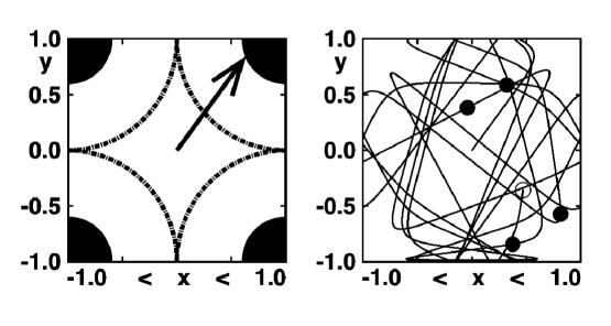
Figure 1: The periodic $2\times 2$ unit cell is shown at the left. The black regions, with potential energy greater than one half, are inacessible to the wanderer particle. Initially the wanderer is at the origin with velocity $(0.6,0.8)$. Outside the central diamond-shaped region the fixed scatterers at the cell corners exert repulsive forces on the wanderer particle. A visually-accurate trajectory, calculated with a quadruple-precision fifth-order Runge-Kutta integrator, using five million timesteps and $dt=0.00001$, is shown at the right with filled circles marking the configurations at times 10, 20, 30, and 40. The open circle corresponds to the maximum time $t=50$.

In the following Sections we describe the specially-smooth differential equations governing the motion of the wandering cell-model particle, and then quantify the algorithmic accuracy with which Leapfrog and the six more sophisticated integrators “solve” this same problem. Our conclusions make up the final Summary section.

II The Cell Model Trajectory in Two Space Dimensions

Cell models played a role in models of the liquid state long before the development of molecular dynamics.b4 The geometry treated here is shown at the left in Figure 1. A mass point, the “wanderer” particle, moves in a periodic square cell with a motionless fixed particle at each of the four vertices. Using periodic boundary conditions the equations of motion are :

$$\dot{x}=(p_{x}/m)\ ;\ \dot{y}=(p_{y}/m)\ ;\ \dot{p}_{x}=F_{x}\ ;\ \dot{p}_{y}=F_{y}\ .$$

The force on the wanderer is the gradient of the potential function $\Phi$ , a sum over the contributions of the four corner scatterers located at $\{\ r_{i}\ \}$ :

$$\Phi=\sum_{1}^{4}[\ 1-(r-r_{i})^{2}\ ]^{4}{\rm\ for\ }|r-r_{i}|<1\ .$$

After advancing the coordinates one timestep $dt$ it is convenient to localize the motion to the cell centered on the origin. Whenever the wanderer moves “out”, we replace it “in” the basic $2\times 2$ unit cell as follows :

$$x<-1\rightarrow x=x+2\ ;\ x>+1\rightarrow x=x-2\ ;\$$

$$y<-1\rightarrow y=y+2\ ;\ y>+1\rightarrow y=y-2\ .$$

We choose initial conditions $\{\ x,y,p_{x},p_{y}\ \}=\{\ 0.0,0.0,0.6,0.8\ \}\$ and show an accurate benchmark solution of the motion equations for a time of 50 at the righthandside of Figure 1 . At times of 10, 20, 30, 40, and 50 the benchmark values of $(x,y)$ are :

10: +0.321356333887505, +0.585921713605895

20: +0.81481797353866, -0.572042192203162

30: -0.040449409487, +0.38290501902

40: +0.3742439, -0.842854

50: +0.4696, -0.3568

Figure 1 shows a unit cell of a periodic two-dimensional lattice in which a single particle moves in the field of scattering particles arranged in a fixed square lattice with nearest-neighbor spacing of 2. The potential energy maximum of unity is twice the energy of the initial condition, shown at the center of the cell. The benchmark solution of the motion equations $\{\ \dot{q}=p\ ;\ \dot{p}=F(q)\ \}$ is shown at the right. This same accurate trajectory was obtained with both the Candy-Rozmus fourth-order and a Runge-Kutta fifth-order integrator using 50 million and 500 million timesteps, respectively. The two trajectories agree throughout within visual accuracy. At a time of 50 $(x,y,p_{x},p_{y})$ are :

$$(x,y,p_{x},p_{y})=(+0.46961,-0.35683,+0.11945,+0.98408)\ {\rm[\ CR4\ ]}\ ;$$

$$(x,y,p_{x},p_{y})=(+0.46962,-0.35682,+0.11948,+0.98408)\ {\rm[\ RK5\ ]}\ .$$

III Seven Typical Integrators and Their Trajectories

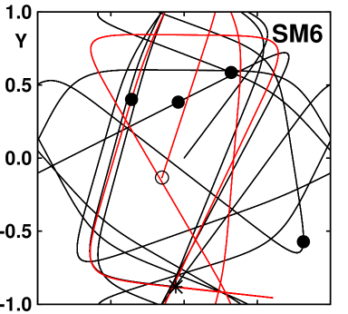
Figure 5: This double-precision trajectory is based on Yoshida’s time-reversible sixth-order integrator with a timestep $dt=0.001$ . There is a color change at $t=36$ , indicating the degradation of trajectory accuracy to $\pm 0.01$ despite the negligible energy error in the fourteenth decimal place. Trajectory reversal at a time of 42 returns to the origin within coordinate errors of 0.01.

We consider seven solution algorithms for the wanderer particle trajectory, [1] Leapfrog (symplectic), [2] Fourth-Order Candy-Rozmus Symplectic, [3] Monte Carlo Symplectic, [4] Sixth-Order Symplectic, [5] Fourth-Order Runge-Kutta, [6] Fifth-Order Runge-Kutta, and [7] Eighth-Order Schlier-Seiter-Teloy Symplectic. For the first six of these we use a fixed timestep typical of “accurate” molecular dynamics simulations $dt=0.001$ . Solutions for those six integrators appear in Figures 2-7 . The particle mass is unity and the energy $\Phi+K$ is one half. For the last integrator, which has a trajectory visually identical to that of Figure 1 we have chosen timesteps as small as 0.00000001 in order to obtain ten-digit accuracy in the wanderer trajectory up to a time of 50 . Let us consider the details of all the integrators next.

III.1 Second-Order Time-Reversible Leapfrog Algorithm

“Symplectic” integratorsb5 ; b6 ; b7 ; b8 ; b9 automatically obey Liouville’s Theorem by advancing the solution of Hamiltonian problems in time according to a series of phase-volume-conserving shears. Symplectic algorithms alternate steps advancing the coordinates and momenta in time. The simplest example is equivalent to the Störmer-Verlet “leapfrog algorithm” :b8 ; b9 ; b10

$$\{\ {\tt q=q+(p*dt/2)\ ;\ p=p+(F/m)*dt\ ;\ q=q+(p*dt/2)}\ \}\longleftrightarrow$$

$$\{\ q_{n+1}-2q_{n}+q_{n-1}\equiv(F/m)_{n}\ \}\ .$$

This algorithm is said to be “second order”b10 , with a fixed-time coordinate error of order $tdt^{2}$ for $t<<2\pi/dt^{2}$ when applied to the simple harmonic oscillator. It is time reversible in that changing $+dt\rightarrow-dt$ gives the same trajectory points either forward or backward in time.

How does the simulation begin? Starting out at the origin, with the wanderer speed equal to unity and a fixed timestep $dt=0.001$, the first 420 steps leave the momenta unchanged and $r^{2}$ becomes 1.0004. During the 421st step the upper right scatterer is contacted and begins to repel the wandering particle with a force :

$$F_{x}=8(x-1)(1-r^{2})^{3}\ ;\ F_{y}=8(y-1)(1-r^{2})^{3}\ ;\ r=(1-x,1-y)\ ,$$

where $x$ and $y$ are the wanderer coordinates.

After an elapsed time $t$ we reverse the sign of the time so as to integrate backward to see how closely the wanderer returns to its initial location. So long as $t<47$ we find that the trajectory reverses to within a distance 0.01 of the origin. We will see that this retracing of steps does not guarantee a match with the accurate trajectory shown at the right in Figure 1. Both the trajectory reversal and the conservation of energy are poor diagnostics for trajectory accuracy, where accuracy means reproducing correct values of the coordinates $x(t),y(t)$ .

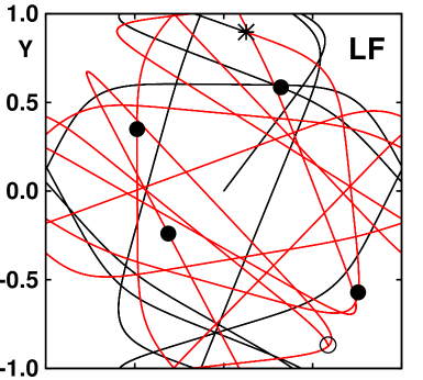
Figure 2: The Leapfrog integrator reproduces the accurate $x$ and $y$ coordinates within 0.01 for an integration time of 18. The energy at that point ( where the trajectory color changes, indicated by a star ) is in error in the seventh decimal place. Here and elsewhere the cited double-precision times are truncated to integers because different implementations, such as varying the order of the operations, could change these numbers.

III.2 Fourth-Order Time-Reversible Symplectic Integrator

Higher-order algorithms, with fixed-time integration errors of order $dt^{3}$, $dt^{4}$, $dt^{5}$ …can be developed from Taylor’s series about $t$ giving small increments in the coordinates and momenta as three-, four-, five- …term series in $dt$ . Candy and Rozmus’ fourth-order integrator (with an error of order $dt^{4}$ at a fixed not-too-large, time) is a simple example, cited in the very useful summary paper by Gray, Noid, and Sumpterb7 :

$${\tt q=q+0.6756036p*dt\ ;\ p=p+1.3512072(F/m)*dt\ ;}$$

$${\tt q=q-0.1756036p*dt\ ;\ p=p-1.7024144(F/m)*dt\ ;\ q=q-0.1756036p*dt\ ;}$$

$${\tt p=p+1.3512072(F/m)*dt\ ;\ q=q+0.6756036p*dt\ .}$$

Reference 7 gives the analytic forms of all of the coefficients. Notice that the coefficients incrementing the coordinates sum to unity as do also those incrementing the momenta. Each timestep requires three separate evaluations of the forces.

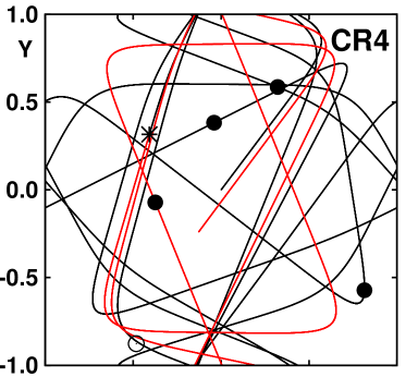
Figure 3: The Candy-Rozmus fourth-order symplectic trajectory exhibits a color change at a time of 34, the maximum for which the coordinate errors are less than 0.01 . The energy error at that time is in the twelfth decimal place. The maximum time at which a reversed trajectory returns to the origin within 0.01 is $t=42$ .

III.3 Monte-Carlo Time-Reversible Symplectic Integrator

Although it is usual to provide coefficients in integration algorithms to many significant figures, in most cases an approximate rendition is sufficient. It is quite possible to develop algorithms with a Monte Carlo method, adjusting the coefficients to minimize the trajectory error for the simple harmonic oscillator problem. An integrator requiring five force evaluations per timestep was developed by Monte Carlo samplingb6 adjusting the coefficients subject to the constraints of time reversibility and normalization so that the Monte Carlo trajectory optimization occurs in a four-dimensional space. The resulting integrator was successful in modelling many-body dynamics but is here applied to the cell-model problem of Figure 1 :

$${\tt q=q+0.005904p*dt\ ;\ p=p+0.171669(F/m)*dt\ ;}$$

$${\tt q=q+0.5l5669p*dt\ ;\ p=p-0.516595(F/m)*dt\ ;}$$

$${\tt q=q-0.021573p*dt\ ;\ p=p+1.689852(F/m)*dt\ ;\ q=q-0.02l573p*dt\ ;}$$

$${\tt p=p-0.516595(F/m)*dt\ ;\ q=q+0.5l5669p*dt\ ;}$$

$${\tt p=p+0.171669(F/m)*dt\ ;\ q=q+0.005904p*dt\ .}$$

The cell model trajectory using this Monte Carlo integrator is illustrated in Figure 4.

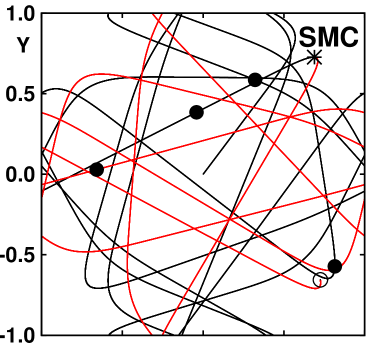
Figure 4: The color change in the trajectory from the Monte Carlo symplectic integrator occurs at a time of 31, after which the coordinate errors exceed 0.01. The energy error there is in the thirteenth digit. For this integrator a trajectory reversed at a time of 43 will return to the origin with coordinates recurring within 0.01.

III.4 Yoshida’s Sixth-Order Time-Reversible Integrator

Yoshida developed and applied a general technique for finding a variety of higher-order symplectic integrators.b11 His sixth-order time-reversible integrator advances the coordinates $(\Delta q\propto pdt)$ eight times per timestep, using the symmetric (so as to guarantee time-reversibility) set of eight coefficients which sum to unity :

$$+0.39225680523878,+0.51004341191846,-0.47105338540976,+0.06875316825252,$$

$$+0.06875316825252,-0.47105338540976,+0.51004341191846,+0.39225680523878.$$

Between the successive coordinate updates there is a force calculation and an update of the momenta $(\Delta p\propto Fdt)$, using seven coefficients, which likewise sum to unity :

$$+0.78451361047756,+0.23557321335936,-1.1776799841789,+1.3151863206839,$$

$$-1.1776799841789,+0.23557321335936,+0.78451361047756.$$

III.5 Fourth-Order and Fifth-Order Runge-Kutta Integrators

Runge-Kutta integrators ( circa 1900, as described in Wikipedia ) advance both coordinates and momenta simultaneously in a series of stages within each timestep $dt$. As in the symplectic case the variables at time $t+dt$ are expressed as series in $dt$, putting conditions on the summed-up coefficients for each power of $dt$ to be treated correctly by the algorithm.

The main advantage of Runge-Kutta methods is that they can be applied to arbitrary sets of ordinary differential equations, not just those from Hamiltonian mechanics. The fourth-order “classic” Runge-Kutta method has been a standard workhorse model for solving sets of coupled ordinary differential equations for 100 years. Applied to the harmonic oscillator the fourth-order algorithm suffers a loss in energy proportional to the fifth power of the timestep. The fifth-order Runge-Kutta integrator behaves in the opposite manner with the energy increasing rather than decreasing.

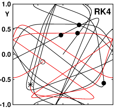
Figure 6: The fourth-order Runge-Kutta trajectory using double precision and a timestep $dt=0.001$ provides coordinates accurate within 0.01 through a time of 35, indicated by the color change at the star. The energy error at that point, $10^{-13}$, is negligible. Changing the sign of the timestep at $t=42$ , $+dt\rightarrow-dt$ , returns the trajectory to the origin within a precision of 0.01 .

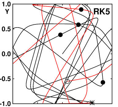
Figure 7: The fifth-order Runge-Kutta trajectory using double precision and a timestep $dt=0.001$ provides coordinates accurate within 0.01 through a time of 37, indicated by the color change at the star. The energy error at that point is $10^{-14}$ . For times less than 42 reversing the trajectory, by setting $+dt\rightarrow-dt$ , returns the trajectory to the origin with precision 0.01. This integrator is the best of the double-precision integrators tested here. Any one of the five higher-order integrators is accurate for about twice the time of the second-order Leapfrog integrator.

Hybrid “adaptive” models, incorporating both fourth- and fifth-order algorithms, provide a simple means for the automatic control of integration errors. The harmonic oscillator is an excellent test case of integrator accuracy where Lyapunov instability is absent.b10 Figure 6 illustrates the same cell-model orbit for the classic fourth-order Runge-Kutta integrator. Figure 7 shows a fifth-order Runge-Kutta integrator :

$$\noindent{\tt yp1=yp[\ y\ ]}$$

$${\tt yp2=yp[\ y+(dt/2)*yp1\ ]}$$

$${\tt yp3=yp[\ y+(dt/16)*(3yp1+yp2)\ ]}$$

$${\tt yp4=yp[\ y+(dt/2)*yp3\ ]}$$

$${\tt yp5=yp[\ y+(dt/16)*(-3yp2+6yp3+9yp4)\ ]}$$

$${\tt yp6=yp[\ y+(dt/7)*(yp1+4yp2+6yp3-12yp4+8yp5)\ ]}$$

$${\tt y=y+(dt/90)*(7yp1+32yp3+12yp4+32yp5+7yp6)}$$

Here yp[  ...  ] represents the righthandside of the vector differential equation $\dot{y}=y^{\prime}$ where the six force evaluations in each timestep are indicated by $\{\ yp1,\ yp2,\ \dots\ yp6\ \}$ .

Both Runge-Kutta integrators return to the origin with errors no more than 0.01 with reversal at time 42. Forward in time their trajectories are accurate through times of 35 and 37, the last being the best of the double-precision integrators. The energy errors for the two Runge-Kutta integerators are in the thirteenth and fourteenth decimal places.

III.6 An Eighth-Order Time-Reversible Symplectic Integrator

Ernst Teloy, Christoph Schlier, and Ansgar Seiter developed and implemented a useful eighth-order time-reversible symplectic integrator with 17 force evaluations per step. Applied to the harmonic oscillator the rms coordinate error increases by about eight orders of magnitude when the timestep is increased by a factor of ten, consistent with an eighth-order method.

For the reader’s convenience we reproduce here the 18 coefficients required to implement the method. They can be found quoted to 35 decimal places at Christoph Schlier’s Freiburg website or in Reference 12 . This precision is steadily reduced, digit by digit, through Lyapunov instability, described in more detail in Section IV. In the cell-model case the rate of precision loss is 0.7 , one binary bit per unit time. Accordingly, for the eighth-order integrator in quadruple precision at time 50 we would expect an exponentially amplified error of order $10^{-32}\times 2^{50}\simeq 10^{-17}$ . In fact, we find a trajectory error of order $10^{-10}$ using a timestep of $10^{-8}$ , as is shown below.

Even so the eighth-order integrator with $dt=0.001$ loses only seven of the original 35 digits in energy along with twenty digits in position when run forward and backward for 50,000 steps to match the time illustrated in all the Figures. As was illustrated and emphasized in References 12 and 13 energy conservation and trajectory reversibility are both of them misleading diagnostics of trajectory accuracy. It is only through a study of convergence that trajectories can be validated. For the eighth-order symplectic integrator the timestep dependence of the $(x,y)$ coordinates at time 50 is as follows :

$$dt=0.00100000\rightarrow(0.48704\ 51729,\ +0.13435\ 10401)$$

$$dt=0.00010000\rightarrow(0.48185\ 80396,\ -0.32559\ 07485)$$

$$dt=0.00001000\rightarrow(0.46961\ 32018,\ -0.35683\ 11339)$$

$$dt=0.00000100\rightarrow(0.46961\ 40145,\ -0.35682\ 95856)$$

$$dt=0.00000010\rightarrow(0.46961\ 40143,\ -0.35682\ 95861)$$

$$dt=0.00000001\rightarrow(0.46961\ 40142,\ -0.35682\ 95862)$$

For the convenience of the reader we reproduce the integrator coefficients here from Reference 12, together with a short harmonic-oscillator program to demonstrate their use.

III.7 Schlier-Seiter-Teloy Integrator Coefficients

c( 1) = +0.04463 79505 23590 22755 91399 96257 33590 d00
c( 2) = +0.13593 25807 16909 59145 54326 42134 95574 d00
c( 3) = +0.21988 44042 71470 72254 44553 50696 06167 d00
c( 4) = +0.13024 94678 05238 28601 62119 37781 96846 d00
c( 5) = +0.10250 36569 39750 69608 26124 10077 79814 d00
c( 6) = +0.43234 52186 93585 47487 98325 78848 77035 d00
c( 7) = -0.00477 48291 69168 81658 02248 90639 62934 d00
c( 8) = -0.58253 47690 40408 45493 11283 79308 61212 d00
c( 9) = -0.03886 26428 21118 17697 73742 08751 89743 d00
c(10) = +0.31548 72853 79404 79698 27360 37972 74199 d00
c(11) = +0.18681 58374 32971 55471 52615 35039 72746 d00
c(12) = +0.26500 27549 90620 83398 34600 29630 79872 d00
c(13) = -0.02405 08473 57473 61993 57358 79824 07554 d00
c(14) = -0.45040 49249 97722 51180 92289 67121 51891 d00
c(15) = -0.05897 43301 55923 86914 57532 39267 66330 d00
c(16) = -0.02168 47617 18613 35324 93438 86847 07580 d00
c(17) = +0.07282 08003 35901 28173 76189 26412 34244 d00
c(18) = +0.55121 42963 41970 67334 40560 13815 94315 d00
Oscillator program with q,p,dt and 18 c(i) :
do i = 1,17,2
q = q + c(i)*p*dt
p = p - c(i+1)*q*dt
enddo
do i = 17,1,-2
q = q + c(i)*p*dt
if(i.gt.1) p = p - c(i-1)*q*dt
enddo

IV Lyapunov Instability in the Cell Model

For chaotic systems the algorithmic accuracy of numerical integrators deteriorates exponentially rather than linearly in the timeb3 . The underlying exponential Lyapunov instability of dynamical systems is easily measured by following the motion of a “reference” trajectory in the usual way, for instance with any one of the seven algorithms discussed here. An additional “satellite” trajectory, separated from the reference by a small length $\delta_{0}$ , is also followed using the same algorithm. At the end of each timestep the separation is rescaled, maintaining the length of the offset between the trajectories constant, but allowing the direction to vary :

$$\delta(t+dt)\equiv[\ r_{s}(t+dt)-r_{r}(t+dt)\ ]\ ;\$$

$$r_{s}\longrightarrow r_{r}(t+dt)+\delta(t+dt)[\ \delta_{0}/|\ \delta(t+dt)\ |\ ]\ .$$

The largest Lyapunov exponent is simply the average value of the growth rates measured at the ends of every timestep prior to rescaling :

$$\lambda_{1}=\langle\ (1/dt)\ln[\ |\ \delta(t+dt)\ |/\delta_{0}\ ]\ \rangle\ .$$

Previous studies of this cell model,b3 with the same initial condition, have shown that the largest Lyapunov exponent is about 0.7. This means that an error of the order $10^{-16}$ at the initiation of a run of length 50 will increase by a factor of $e^{\lambda t}=e^{0.7\times 50}=e^{35}\simeq 10^{15}\$.

This exponential growth rate explains why it is that all of the double-precision integrators fail, from the standpoint of reproducing a reversible trajectory, at about the same time, at about half the time where quadruple-precision trajectories fail. It is because these trajectories are just approximations that the most sophisticated biomolecule simulations are based on the rudimentary leapfrog algorithm rather than more sophisticated algorithms.

Of course, even the slightest difference in the error prior to amplification will yield a different history. Just summing the particle interactions in a different order leads to qualitatively different histories once the Lyapunov instability rises to the level of visibility, an increase of 16 digits for routine double-precision simulations. The phase-shift errors in all of the algorithms discussed here can be measured by choosing the initial velocity $(\sqrt{1/2},\sqrt{1/2})$ for which the roundoff errors in the $x$ and $y$ directions are identical.

If high accuracy is required, as in astronomical simulations, multiple precision can be employed, as demonstrated by Lorenz Attractor simulations using a precision of thousands of decimal digits. But, as Joseph Ford was fond of pointing out, Lyapunov instability is incompatible with high accuracy. Doubling the number of significant figures in the integration algorithm only doubles the time for which the simulation is accurate.

Recently Hanno Rein and David Siegelb14 developed and implemented a relatively complicated fifteenth-order integrator for gravitational problems with the provocative title “A Fast, Adaptive, High-Order Integrator for Gravitational Dynamics, Accurate to Machine Precision Over a Billion Orbits”. Evidently this integrator is not at all intended for long-time applications to chaotic problems, where errors grow exponentially with time. Conversations with Ben Leimkuhler and Mark Tuckerman, both of whom summarily dismiss the use of Runge-Kutta techniques, due to their monotonic energy drift, plus the appearance of Rein and Siegel’s high-order long-time work led to the present article.

V Recent Developments and Summary

To summarize, for simple chaotic simulations ( such as classical fluids ) symplectic integrators attain accuracies similar to those obtained with Runge-Kutta integration and are primarily limited by Lyapunov instability. Although energy conservation and trajectory reversibility characterize symplectic integrators, those properties do not ensure trajectory accuracy. The reversibility of the double-precision leapfrog integrator, to a time of 47 and back, exceeds that of all the more accurate double-precision integrators.

For us it was illuminating to find that the humble Leapfrog integrator, presumably nearing its 330th anniversaryb8 , is nearly as useful as are its more complex relatives, and is certainly far more economical. For higher accuracy there is little distinction between the symplectic and the Runge-Kutta integrators for chaotic problems, because both types lose accuracy at the very same rate, determined by the maximum Lyapunov exponent.

It is significant that all of the integrators used here conserve energy almost perfectly for the benchmark problem. They also reverse back to the initial conditions even when their trajectories are inaccurate. One takeaway message from these simulations is the one to which Joseph Ford devoted much thought and many thought-provoking words, among them these taken from Reference 16 :

“Newtonian determinism assures us that chaotic orbits exist and are unique, but they are nevertheless so complex that they are humanly indistinguishable from realisations of truly random processes.”

Liao has confronted the Lyapunov instability problem headon for the Lorenz Attractor.b17 By using 3500-term series expansions coupled with 4180-digit arithmetic he followed the evolution of the Lorenz Model to a time of 10,000. Like the continuing discovery of the digits of $\pi$ this activity will last as long as mankind.

Lyapunov instability often shows up in peculiar places. Simply changing the order of operations in adding up forces or in computing the weights of contributions to differential equations’ righthandsides can provide the seeds from which macroscopic change develops. We learned this lesson in simulating the collisions of mirror-image manybody drops and crystals. To retain accurate mirror symmetry it was necessary to symmetrize the force calculations at every timestep.b18

VI Acknowledgments

We thank Ben Leimkuhler, Hanno Rein, and Mark Tuckerman for their useful and stimulating comments, Clint Sprott for his constant encouragement, and Christoph Schlier for several helpful emails. We are grateful to the GNU Fortran project for furnishing their no-cost quadruple-precision compiler. To find it GOOGLE “GNU Fortran project”.

References

- (1) M. Karplus, “ ‘Spinach on the Ceiling’ : a Theoretical Chemist’s Return to Biology”, Annual Review of Biophysics and Biomolecular Structure 35, 1-47 (2006).
- (2) H. A. Posch, W. G. Hoover, and F. J. Vesely, “Canonical Dynamics of the Nosé Oscillator: Stability, Order, and Chaos”, Physical Review A 33, 4253-4265 (1986).
- (3) W. G. Hoover and C. G. Hoover, Simulation and Control of Chaotic Nonequilbrium Systems (World Scientific Publishers, Singapore, 2015).
- (4) J. A. Barker and D. Henderson, “What is ‘Liquid’ ? Understanding the States of Matter”, Reviews of Modern Physics 48, 587-671 (1976).
- (5) B. Leimkuhler and S. Reich, Simulating Hamiltonian Dynamics (Cambridge University Press, United Kingdom, 2004).
- (6) W. G. Hoover, O. Kum, and N. E. Owens [ now Nancy Fulda ], “Accurate Symplectic Integrators via Random Sampling”, the Journal of Chemical Physics 103, 1530-1532 (1995).
- (7) S. K. Gray, D. W. Noid, and B. G. Sumpter, “Symplectic Integrators for Large Scale Molecular Dynamics Simulations: A Comparison of Several Explicit Methods”, the Journal of Chemical Physics 101, 4062-4072 (1994).
- (8) E. Hairer, C. Lubich, and G. Wanner, “Geometric Numerical Integration Illustrated by the Störmer-Verlet Method”, Acta Numerica 12, 399-450 (2003).
- (9) D. Levesque and L. Verlet, “Molecular Dynamics and Time Reversibility”, Journal of Statistical Physics 72, 519-537 (1993).
- (10) G. D. Venneri and W. G. Hoover, “Simple Exact Test for Well-Known Molecular Dynamics Algorithms”, Journal of Computational Physics 73, 468-475 (1987).
- (11) H. Yoshida, “Construction of Higher Order Symplectic Integrators”, Physics Letters A 150, 262-268 (1990).
- (12) Ch. Schlier and A. Seiter, “High-Order Symplectic Integration: An Assessment”, Computer Physics Communications 130, 176-189 (2000).
- (13) Ch. Schlier and A. Seiter, “Symplectic Integration of Classical Trajectories: A Case Study”, Journal of Physical Chemistry 102, 9399-9404 (1998).
- (14) H. Rein and D. S. Spiegel, “IAS15: A Fast, Adaptive, High-Order Integrator for Gravitational Dynamics, Accurate to Machine Precision Over a Billion Orbits”, ariv 1409.4779, also available in the Monthly Notices of the Royal Astonomical Society.
- (15) W. G. Hoover, J. C. Sprott, and P. K. Patra, “Ergodic Time-Reversible Chaos for Gibbs’ Canonical Oscillator”, (submitted to Physical Review E, 2015) = ariv 1503.06729.
- (16) J. Ford, “What is Chaos, that We Should be Mindful of I≈ß≈çt ?”, in The New Physics, edited by Paul Davies (Cambridge University Press, 1989).
- (17) S. Liao, “A Comment on the Arguments about the Reliability and Convergence of Chaotic Simulations”, International Journal of Bifurcation and Chaos, 24, 91450119 (2014) = ariv 1401.0256.
- (18) W. G. Hoover and C. G. Hoover, “What is Liquid? Lyapunov Instability Reveals Symmetry-Breaking Irreversibility Hidden within Hamilton’s Many-Body Equations of Motion”, Condensed Matter Physics 18, 13003-1-13 (2015) = ariv 1405.2485.