hep-th/yymm.nnnn

Filling The Gaps With PCO’s
Ashoke Sen¹ and Edward Witten^2
1Harish-Chandra Research Institute, Chhatnag Road, Jhusi, Allahabad 211019, Indis ²School of Natural Sciences, Institute for Advanced Study, Princeton NJ USA 08540

Superstring perturbation theory is traditionally carried out by using picture-changing operators (PCO’s) to integrate over odd moduli. Naively the PCO’s can be inserted anywhere on a string worldsheet, but actually a constraint must be placed on PCO insertions to avoid spurious singularities. Accordingly, it has been long known that the simplest version of the PCO procedure is valid only locally on the moduli space of Riemann surfaces, and that a correct PCO-based algorithm to compute scattering amplitudes must be based on piecing together local descriptions. Recently, “vertical integration” was proposed as a relatively simple method to do this. Here, we spell out in detail what vertical integration means if carried out systematically. This involves a hierarchical procedure with corrections of high order. One might anticipate such a structure from the viewpoint of super Riemann surfaces.

1 Introduction

Superstring perturbation theory is traditionally constructed in an elegant framework of superconformal field theory, with insertions of picture-changing operators (PCO’s) as well as vertex operators for physical states [1]. The PCO’s give a method of integration over the odd moduli of a super Riemann surface [2].

Naively, the PCO’s can be inserted at arbitrary positions on a superstring worldsheet, but it has been known since the 1980’s that this is oversimplified. The measure on the moduli space of Riemann surfaces that is constructed using PCO’s has spurious singularities if two PCO’s collide, and also if a certain global condition is obeyed. For this paper, it suffices to know that the locus of spurious singularities is of complex codimension 1 or real codimension 2 and has a reasonable behavior at infinity on moduli space. Actually, the locus of spurious singularities is rather complicated and appears to have few useful properties beyond what we have just stated.

To get a correct, gauge-invariant method of computing superstring scattering amplitudes, it is desirable to avoid spurious singularities. For topological reasons, a choice of PCO locations that avoids spurious singularities exists only locally on moduli space. Accordingly, it has been understood since the 1980’s that a correct method of computation based on PCO’s has to be based on piecing together local descriptions.

A relatively simple method to piece together the local descriptions was proposed recently [3] in the form of “vertical integration.” However, only the basic idea of vertical integration was described. Here, we explain systematically what vertical integration means if carried out in full. An inductive procedure is involved with corrections, in a certain sense, of all orders (bounded by the number of PCO’s). The need for corrections of high order may come as a surprise to some readers. However, this should be anticipated based on what was understood in the old literature, and is fairly clear from the point of view of super Riemann surfaces.

In section 2, we recall the basic idea of vertical integration. In section 3, we describe the procedure systematically to all orders. The construction described in section 3 requires making some choices for the “vertical segment,” and in section 4 we show that the scattering amplitude is independent of these choices. The measure that the procedure of section 3 generates on the moduli space of ordinary Riemann surfaces is discontinuous, and this is compensated by additional terms that take the form of integrals over subspaces of the moduli space of codimension $\geq 1$. In section 5, we describe a generalization of this procedure that generates a smooth measure on the moduli space and show that the procedure described in section 3 can be regarded as a special case of this. In section 6, we show gauge invariance of the amplitude defined in section 5. In section 7, we explain why the inductive or hierarchical procedure that we follow would be expected from the point of view of super Riemann surfaces.

In this paper, we ignore the fact that the moduli space $M$ of Riemann surfaces is not compact. This noncompactness arises from the fact that the string worldsheet $\Sigma$ can degenerate, and is associated to the infrared behavior of string theory. This infrared behavior has been much analyzed in the literature and will not be considered here. We simply remark that everything we say must be supplemented with some fairly well-known conditions on the behavior of PCO’s in the limit that $\Sigma$ degenerates.

A hierarchy of corrections somewhat similar to what we describe here was used in [6] to construct a field theory of the NS sector of superstring theory. Each string field theory diagram parametrizes in a relatively simple way a piece of the moduli space of bosonic Riemann surfaces and comes with a relatively natural choice of PCO insertions suitable for that piece. On the boundaries of the parts of moduli space parametrized by different diagrams, the PCO choices do not fit together properly. In [6], a hierarchy of corrections was introduced to compensate for this.

2 Overview

Before describing vertical integration in its most general form, we shall discuss some simple cases explicitly and explain the issues one faces in extending to more general cases. Let us denote by ${\mathcal{X}}(z)$ the PCO inserted at the point $z$ in a string worldsheet $\Sigma$. We can express this as

$${\mathcal{X}}(z)=\{Q_{B},\xi(z)\}\,,$$ (2.1)

where $\xi(z)$ is a fermion field of dimension (0,0) that arises from the bosonization of the superghost system. $\xi(z)$ is an operator defined in the large Hilbert space of Friedan, Martinec, and Shenker [1]. We shall work in the small Hilbert space, where one removes the zero-mode of $\xi$ from the spectrum of operators, so that only the derivatives of $\xi$ are valid operators. All our analysis will involve only such operators. However, we shall make use of the fact that the periods of the closed 1-form $\partial\xi$ vanish on any Riemann surface, even in the presence of punctures labeled by operators of the small Hilbert space. Thus operators of the form $\xi(u)-\xi(v)\equiv\int_{v}^{u}\partial\xi(z)dz$ are well defined in the small Hilbert space without having to specify the contour of integration from $u$ to $v$.

Now consider a situation where the moduli space $M$ over which we integrate has real dimension $n$ and suppose further that the correlation function of interest requires insertion of only one PCO. Each point $m\in M$ determines a Riemann surface $\Sigma(m)$, and the one PCO that we need can be inserted at an arbitrary point $z\in\Sigma(m)$ except that we must avoid a bad set of (real) codimension 2 at which there are spurious singularities. As $\Sigma(m)$ has dimension 2, the bad set consists of finitely many points in each $\Sigma(m)$.

We denote by $Y$ a fiber bundle with base $M$ and fiber $\Sigma(m)$:

$$\begin{matrix}\Sigma(m)&{\longrightarrow}&Y\cr&&~{}~{}\Big{\downarrow}\varphi\cr&&M.\end{matrix}$$ (2.2)

We also denote as $X$ the subspace of $Y$ in which, in each fiber, one deletes the bad points at which the PCO should not be inserted.

We denote local coordinates on $X$ as $(m;a)$, with $m\in M$ and $a\in\Sigma(m)$. $X$ is not a fiber bundle over $M$, because as one varies $m\in M$, the bad points in $\Sigma(m)$ can collide. However, there certainly is a map $\varphi:X\to M$. This is the map that forgets where the PCO is inserted; in local coordinates, it maps $(m;a)$ to $m$.

Suppose that $M$ is of real dimension $n$. The path integral with one PCO insertion at $a\in M(m)$ (and all external vertex operators on-shell) naturally computes for us a closed $n$-form on $X$:

$$\omega_{n}(m;a)\equiv\left\langle({\mathcal{X}}(a)-\partial\xi(a)da)\wedge{\mathcal{O}}\right\rangle_{n}\,.$$ (2.3)

Here $\langle~{}~{}\rangle$ denotes a CFT correlation function on $\Sigma(m)$; ${\mathcal{O}}$ is a formal sum of operator-valued $k$-forms on $M$ for all $k$ between 0 and $n$, constructed from insertions of $b$-ghosts and possible on-shell vertex operators for external states. The subscript $n$ denotes that we have to extract the $n$-form part of this expression. The precise form of ${\mathcal{O}}$ and the procedure to extract the closed $n$-form $\omega_{n}(m;a)$ is well-known and will not be described here.

The subtlety of superstring perturbation theory in the PCO formalism arises because the PCO formalism naturally constructs a closed $n$-form on $X$, not on $M$. Ideally one would want an $n$-form on $M$, which would automatically be closed for dimensional reasons, and which would be integrated over $M$ to compute a scattering amplitude.

How can we eliminate the dependence on $a$? If we had a section $s:M\to X$ of the map $\varphi:X\to M$, which concretely would be given in local coordinates by a formula $a=s(m)$, then we could pull back $\omega_{n}(m;a)$ to an $n$-form on $M$ and define the scattering amplitude as

$$\int_{M}s^{*}(\omega_{n})=\int_{M}\omega_{n}(m,s(m)).$$ (2.4)

Since $\omega_{n}$ is closed, this definition of the scattering amplitude is invariant under small changes in $s$. (From this point of view, if there are topologically distinct choices of $s$ they might lead to different but equally well-defined results for the scattering amplitude.) Moreover, $\omega_{n}$ and therefore $s^{*}(\omega_{n})$ changes by an exact form if one makes gauge transformations for some of the external vertex operators, so the scattering amplitude defined this way would be gauge-invariant.

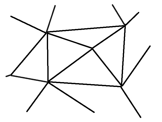
Figure 1: A triangulation of a two-dimensional surface.

In general, the map $\varphi$ does not have a global section, but if we choose a sufficiently fine triangulation of $M$ (fig. 1) then on each triangle, there will be a local section. This is just the statement that on a sufficiently small triangle, we can choose the PCO location as a continuous function of $m$ while avoiding the bad points.

Let $T_{1}$ be one such triangle with local section $a=s^{1}(m)$. The contribution to an on-shell amplitude from the triangle $T_{1}$ with the PCO insertion at $a=s^{1}(m)$ can be expressed as

$$\int_{T_{1}}\omega_{n}(m;s^{1}(m)).$$ (2.5)

Now suppose that $T_{2}$ is a second triangle which shares a common boundary $B$ with $T_{1}$, and let $s^{2}$ denote a local section on $T_{2}$. Then the contribution to the amplitude from $T_{2}$, computed with this local section, will be given by

$$\int_{T_{2}}\omega_{n}(m;s^{2}(m))\,.$$ (2.6)

Since $s^{1}(m)$ and $s^{2}(m)$ do not in general agree on the boundary $B$, the full amplitude must be obtained by summing over contributions from different triangles together with appropriate correction factors from the boundaries between the triangles.

Vertical integration is a prescription for determining these corrections. We “fill the gap” in the integration cycle on $Y$ by drawing a vertical segment $U$. $U$ is constructed by connecting the point $s^{1}(m)\in\Sigma(m)$ to $s^{2}(m)\in\Sigma(m)$ by a curve $C(m)\in\Sigma(m)$ for each $m\in B$, keeping away from the spurious singularities, and taking the collection of all such curves: $\{C(m):m\in B\}$. We parametrize $U$ by $m\in B$ and a variable $u\in[0,1]$ that labels the position along the curve $C(m)$. The correction term associated with the boundary $B$ is now taken to be given by the integral of $\omega_{n}(m;a(u))$ over $U$. Using (2.3), the integration over $u$ for fixed $m\in B$ can be performed first, yielding the result

$$\int_{U}\omega_{n}(m;u)=\int_{B}\,\langle(\xi(s^{1}(m))-\xi(s^{2}(m)))\,{\mathcal{O}}\rangle_{n-1}$$ (2.7)

The subscript just means that $\langle(\xi(s^{1}(m))-\xi(s^{2}(m)))\,{\mathcal{O}}\rangle_{n-1}$ is naturally an $(n-1)$-form. Importantly, the right hand side does not depend on the choice of the paths $C(m)$, so we do not really need to pick a specific vertical segment $U$.

In general, $M$ may be triangulated with many triangles $T_{i}$, meeting in common boundaries $B_{ij}=T_{i}\cap T_{j}$ (most of the $B_{ij}$ are empty). The full scattering amplitude is defined to be

$$\sum_{i}\int_{T_{i}}\omega_{n}(m;s^{i}(m))+\int_{B_{ij}}\langle(\xi(s^{i}(m))-\xi(s^{j}(m)))\,{\mathcal{O}}\rangle_{n-1}.$$ (2.8)

Fixing the relative sign between the two terms requires fixing the orientation of $B_{ij}$; this will be done carefully in section 3. Standard arguments show that this formula is invariant under continuous changes of the $T_{i}$ and the $s^{i}$, and also is invariant under gauge transformations of external state.

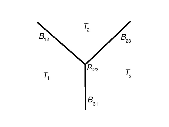
Figure 2: A triple intersection of triangles.

The logic behind this definition is as follows. Over each double intersection $B_{ij}=T_{i}\cap T_{j}$ of triangles, we can define a “vertical segment” $U_{ij}$ as a union of paths from $s^{i}$ to $s^{j}$. Now let us consider a triple intersection $T_{i}\cap T_{j}\cap T_{k}$, with precisely three triangles meeting at a common vertex (fig. 2). This means that $B_{ij}$, $B_{jk}$, and $B_{ki}$ share a common endpoint $p_{ijk}$. (The case of more than three triangles meeting at a vertex can be treated similarly.) It then makes sense to ask if $U_{ij}$, $U_{jk}$, and $U_{ki}$ agree at $p_{ijk}$, i.e. for each $m\in p_{ijk}$ the paths from $s_{i}(m)$ to $s_{j}(m)$ in $U_{ij}$, $s_{j}(m)$ to $s_{k}(m)$ in $U_{jk}$ and $s_{k}(m)$ to $s_{i}(m)$ in $U_{ki}$ together describe zero path. If they do (for all triples $ijk$), then the triangles $s^{i}(T_{i})$ and the vertical segments $U_{ij}$ could be glued together to make a closed cycle $S\subset X$. One would then define the scattering amplitude as $\int_{S}\omega_{n}$. This actually would agree with eqn. (2.6), since under the stated assumptions, $S$ could be slightly perturbed to be a section $s:M\to X$. It would clearly also agree with eqn. (2.8), which expresses the scattering amplitude as an integral over $S=\cup_{i}T_{i}\cup_{jk}U_{jk}$. In reality, it may not possible to make the $U_{ij}$’s agree at triple intersections since there may be a topological obstruction to finding a global section $s$, but because the formula of eqn. (2.8) does not depend on the choices of the $U_{ij}$, this version of the formula makes sense anyway and has the same properties as if the $U_{ij}$ did agree on triple intersections. In fact, we can study each triple intersection independently of the others, and at any one triple intersection, one can arrange so that the $U_{ij}$ do agree.

As long as only one PCO is needed, this is the end of the story. The situation gets more complicated when there are more PCO’s. First of all, the generalization of (2.7) now is ambiguous since $s^{1}(m)$ and $s^{2}(m)$ each will represent a collection of PCO’s, and the integral in (2.7) depends on the order in which we move the PCO’s. Second, we may need additional correction terms from codimension $\geq 2$ subspaces where three or more triangles meet. We can illustrate both these issues by considering the case where we need two PCO insertions in the correlator. In this case the role of $Y$ is played by the bundle whose base is $M$ and whose fiber is $\Sigma(m)\times\Sigma(m)$. As before, $X$ is obtained by excluding from $Y$ certain codimension $2$ subspaces on which we encounter spurious poles. The local coordinates of $X$ can still be denoted as $(m;a)$ but now $a$ stands for a pair of PCO locations $(z_{1},z_{2})$. Similarly the choice of a local section $s^{1}$ on $T_{1}$ will now specify a pair of points $(z_{1}^{(1)}(m)\in\Sigma(m),z_{2}^{(1)}(m)\in\Sigma(m))$ avoiding spurious poles for each $m\in T_{1}$, and the choice of a local section $s^{2}$ on $T_{2}$ will specify a pair of points $(z_{1}^{(2)}(m)\in\Sigma(m),z_{2}^{(2)}(m)\in\Sigma(m))$ avoiding spurious poles for $m\in T_{2}$. The contribution to the amplitude from a given triangle $T_{i}$ is still given as

$$\int_{T_{i}}(s^{i})^{*}(\omega_{n})=\int_{T_{i}}\omega_{n}(m;z_{1}^{(i)}(m),z_{2}^{(i)}(m)),$$ (2.9)

but $\omega_{n}(m;a)$ is now given by

$$\omega_{n}(m;a)\equiv\left\langle({\mathcal{X}}(z_{1})-\partial\xi(z_{1})dz_{1})\wedge({\mathcal{X}}(z_{2})-\partial\xi(z_{2})dz_{2})\wedge{\mathcal{O}}\right\rangle_{n},$$ (2.10)

with two PCO insertions. We can now try to determine the correction terms at the boundaries between triangles by generalizing our prescription for vertical integration. At an intersection of two triangles $T_{1}$ and $T_{2}$, we again need to integrate over a “vertical segment” that fills in between $s^{1}(T_{1})$ and $s^{2}(T_{2})$. For this, from each $m\in B$ we need to connect $(z_{1}^{(1)}(m),z_{2}^{(1)}(m))$ to $(z_{1}^{(2)}(m),z_{2}^{(2)}(m))$ by a path in $\Sigma(m)\times\Sigma(m)$. But now, if we imitate the above procedure, the result will depend on the path. It is easy to check, for example, that the paths

$$(z_{1}^{(1)}(m),z_{2}^{(1)}(m))\to(z_{1}^{(2)}(m),z_{2}^{(1)}(m))\to(z_{1}^{(2)}(m),z_{2}^{(2)}(m))$$ (2.11)

and

$$(z_{1}^{(1)}(m),z_{2}^{(1)}(m))\to(z_{1}^{(1)}(m),z_{2}^{(2)}(m))\to(z_{1}^{(2)}(m),z_{2}^{(2)}(m))$$ (2.12)

give different results for the integral:

$$\int_{B}\bigg{\langle}\left[(\xi(z_{1}^{(1)})-\xi(z_{1}^{(2)}))({\mathcal{X}}(z_{2}^{(1)})-\partial\xi(z_{2}^{(1)})dz_{2}^{(1)})\right.$$

$$\qquad\qquad\left.+(\xi(z_{2}^{(1)})-\xi(z_{2}^{(2)}))({\mathcal{X}}(z_{1}^{(2)})-\partial\xi(z_{1}^{(2)})dz_{1}^{(2)})\right]\wedge{\mathcal{O}}\bigg{\rangle}_{n-1}$$ (2.13)

and

$$\int_{B}\bigg{\langle}\left[(\xi(z_{2}^{(1)})-\xi(z_{2}^{(2)}))({\mathcal{X}}(z_{1}^{(1)})-\partial\xi(z_{1}^{(1)})dz_{1}^{(1)})\right.$$

$$\qquad\qquad\left.+(\xi(z_{1}^{(1)})-\xi(z_{1}^{(2)}))({\mathcal{X}}(z_{2}^{(2)})-\partial\xi(z_{2}^{(2)})dz_{2}^{(2)})\right]\wedge{\mathcal{O}}\bigg{\rangle}_{n-1}$$ (2.14)

where $dz_{i}^{(1)}$, $dz_{i}^{(2)}$ have to interpreted as their pullback to $B$. Let us suppose that we have made some specific choice of the path for each boundary separating a pair of triangles. Now if we consider the subspace of $M$ where three triangles $T_{1}$, $T_{2}$ and $T_{3}$ meet, then the chosen path from $(z_{1}^{(1)}(m),z_{2}^{(1)}(m))\to(z_{1}^{(2)}(m),z_{2}^{(2)}(m))$ on the boundary between $T_{1}$ and $T_{2}$, together with the chosen path from $(z_{1}^{(2)}(m),z_{2}^{(2)}(m))\to(z_{1}^{(3)}(m),z_{2}^{(3)}(m))$ on the boundary between $T_{2}$ and $T_{3}$, may not match the chosen path from $(z_{1}^{(1)}(m),z_{2}^{(1)}(m))\to(z_{1}^{(3)}(m),z_{2}^{(3)}(m))$ on the boundary between $T_{1}$ and $T_{3}$. This means that when we regard the integrals as integrals over subspaces of $Y$, then even after filling the gaps between the sections over $T_{1}$ and $T_{2}$, the sections over $T_{2}$ and $T_{3}$ and the sections over $T_{1}$ and $T_{3}$, we are left with a gap over the common intersection of the three triangles. The earlier argument based on the path independence of (2.7) does not help us since now the result does depend on some details of the path. Thus we now need to “fill this gap,” leading to additional correction terms.

In general, for computing an amplitude with some given numbers of external legs of Neveu-Schwarz or Ramond type and given genus, we need a fixed number $K$ of PCO insertions. The analog of $Y$ in the above discussion is a fiber bundle over $M$ whose fiber is a product $\Xi(m)=\Sigma(m)\times\Sigma(m)\times\dots\times\Sigma(m)$ of $K$ copies of $\Sigma(m)$. The analog of $X$ is obtained by omitting from each fiber of $\Xi(m)$ a codimension 2 subset on which spurious singularities arise. We shall denote a point in $X$ by $(m;a)$ with $m\in M$, $a\in\Xi(m)$ and by $\varphi:X\to M$ the map that forgets $a$. In general, $\varphi:X\to M$ does not have a global section but it has local sections. Thus if we triangulate $M$ (we follow a slightly different procedure in section 3), a local section will exist over each simplex (recall that a simplex is the $n$-dimensional analog of a triangle). We can follow the procedure described above, integrating $(s^{i})^{*}(\omega_{n})$ over each simplex and making corrections on the boundaries of simplices. But now, further corrections will be needed on higher codimension subspaces where the boundaries meet. In general, one needs corrections on codimension $k$ subspaces for all $k\leq K$. The main goal of this paper to give a systematic procedure for constructing these correction terms and to show that once all the corrections are added, the result has the desired properties of the string amplitudes. In particular, it is gauge-invariant and free from any ambiguity.

3 General Procedure

In this section, we shall generalize the ideas of section 2 to arrive at a complete prescription for computing the amplitude.

3.1 Dual Triangulations

For carrying out this program, roughly speaking, we will use a triangulation of $M$, but actually triangulation is not precisely the most convenient notion. To “triangulate” an $n$-manifold $M$ means to build it by gluing together simplices, or simply by triangles if $n=2$. In a triangulation, any number of simplices might meet at a vertex. Instead of triangles, we might cover $M$ by more general polyhedra again in general with any number of building blocks meeting at a vertex. This is sketched in two dimensions in fig. 3. The analog of this in dimension $n$ is to use $n$-dimensional polyhedra, perhaps of some restricted type, as the building blocks, rather than $n$-simplices.

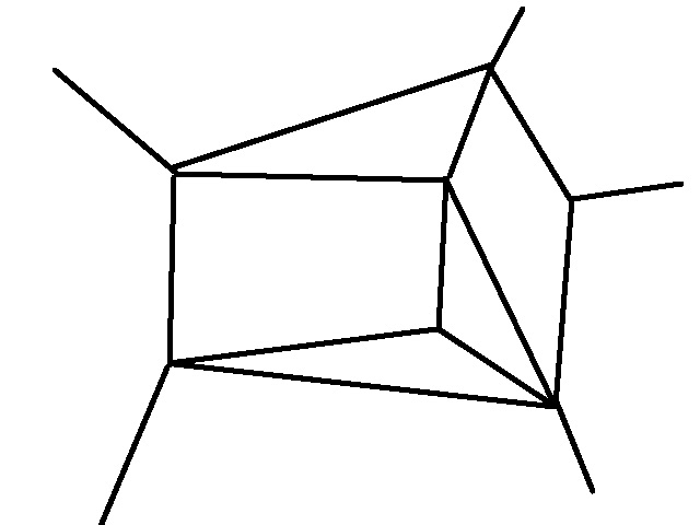
Figure 3: A covering of a two-dimensional surface by more general polygons.

For our purposes, we do not want an arbitrary covering by polyhedra, but the restriction to simplices is also not convenient. We use the fact that to a covering $\Lambda$ by polyhedra, we can associate a dual covering $\widetilde{\Lambda}$. In this duality, faces of dimension $k$ are replaced by faces of dimension $n-k$ that meet them transversely. In two dimensions, this means that a polygon in the covering $\Lambda$ corresponds to a vertex in the dual covering $\widetilde{\Lambda}$, and vice-versa, while the edges $\Lambda$ meet the edges in $\widetilde{\Lambda}$ transversely (fig. 4)).

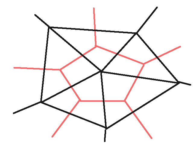
Figure 4: A triangulation (black) and the dual covering (red). We call the dual covering a dual triangulation. Any vertex of one of the polygons making up a dual triangulation is contained in precisely three of those polygons.

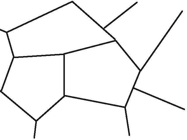
Figure 5: A dual triangulation of a two-dimensional surface is defined by drawing a trivalent graph on the surface.

In the two-dimensional example shown in fig. 4, the “original” covering $\Lambda$ is a triangulation. This means generically that the dual covering $\widetilde{\Lambda}$ is not a triangulation, but a covering by more general polygons. However, $\widetilde{\Lambda}$ has a useful property: every vertex in $\widetilde{\Lambda}$ is contained precisely in three polygons. In two dimensions, a covering of $M$ with this property can be built by drawing a trivalent graph on $M$ (fig. 5)).

If $M$ is a manifold of any dimension $n$, by a “dual triangulation,” we mean a covering that is dual to a triangulation. Thus, if $\Upsilon$ is a dual triangulation of $M$, then it is built by gluing together $n$-dimensional polyhedra along their boundary faces, in such a way that for $k=1,\dots,n$, every codimension $k$ face of one of the polyhedra is contained in precisely $k+1$ polyhedra in $\Upsilon$. This generalizes the fact that in dimension 2, every edge in a dual triangulation is contained in two polygons and every vertex is contained in three polygons. It will be technically easier for us to use a dual triangulation rather than some other type of covering, because it is useful to have a bound on the number of polyhedra that meet at a face of given codimension.

3.2 Basic Setup

We pick a dual triangulation $\Upsilon$ of $M$ by gluing together polyhedra. For $k=0,\dots,n$, let $S_{k}$ be the set of codimension $k$ faces of all the polyhedra that make up $\Upsilon$. So $S_{0}$ is the set of polyhedra, $S_{1}$ is the set of their boundary faces, $S_{2}$ is the set of codimension 2 faces making up the boundaries of the faces in $S_{1}$, and so on. We denote a polyhedron as $M_{0}^{\alpha}$, $\alpha\in S_{0}$, and denote by $M_{k}^{\alpha_{0}\cdots\alpha_{k}}$ the codimension $k$ face that is shared by the codimension zero faces $M_{0}^{\alpha_{0}},\cdots,M_{0}^{\alpha_{k}}$. We pick an orientation on $M$; this restricts to an orientation of each polyhedron $M_{0}^{\alpha}$, $\alpha\in S$. We pick an orientation on $M_{k}^{\alpha_{0}\cdots\alpha_{k}}$ via the relation

$$\partial M_{k}^{\alpha_{0}\cdots\alpha_{k}}=-\sum_{\beta}M_{k+1}^{\alpha_{0}\cdots\alpha_{k}\beta}$$ (3.1)

where the sum over $\beta$ runs over all codimension 0 faces $M_{0}^{\beta}$, distinct from $M_{0}^{\alpha_{0}},\dots,M_{0}^{\alpha_{k}}$, that have nonempty intersection with $M_{k}^{\alpha_{0}\cdots\alpha_{k}}$. These definitions imply that the orientation of $M_{k}^{\alpha_{0}\cdots\alpha_{k}}$ changes sign under $\alpha_{i}\leftrightarrow\alpha_{j}$ for any pair $(i,j)$.

We pick $\Upsilon$ to be fine enough so that the map $\varphi:X\to M$ has a section $s^{\alpha}$ over each of the polyhedra $M_{0}^{\alpha}$, $\alpha\in S_{0}$. We need to impose further conditions on the $s^{\alpha}$. To motivate the needed conditions, we consider the case of just two PCO’s and examine the correction terms (LABEL:ecor1) or (LABEL:ecor2) that are needed on the intersection $M_{1}^{12}=M_{0}^{1}\cap M_{0}^{2}$ of two polyhedra. These depend on two sets of PCO data e.g. $(z_{1}^{(1)}(m),z_{2}^{(1)}(m))$ on $M_{0}^{1}$ and $(z_{1}^{(2)}(m),z_{2}^{(2)}(m))$ on $M_{0}^{2}$. The corrections involve mixed correlation functions involving products $\xi(z_{1}^{(2)}){\mathcal{X}}(z_{2}^{(1)})$ or $\xi(z_{2}^{(1)}){\mathcal{X}}(z_{1}^{(2)})$. To ensure that these are free from spurious singularities, it is not enough that $(z_{1}^{(1)},z_{2}^{(1)})$ and $(z_{1}^{(2)},z_{2}^{(2)})$ separately describe configurations free from spurious singularities; we also require that $(z_{1}^{(1)},z_{2}^{(2)})$ and $(z_{1}^{(2)},z_{2}^{(1)})$ describe configurations with the same property.

In order to describe the required condition for the general case, let us introduce some notation. For some given $m\in M$, let $a^{0},\cdots,a^{k}$ denote $k+1$ possible PCO arrangements, with each $a^{\alpha}$ standing for a set of $K$ points $(z_{1}^{(\alpha)},\cdots z_{k}^{(\alpha)})$ with $z_{i}^{(\alpha)}(m)\in\Sigma(m)$. Now consider the $(k+1)^{K}$ possible arrangement of PCO’s $(z_{1},\cdots z_{K})$ where each $z_{i}$ can take values $z_{i}^{(\alpha_{0})},\cdots z_{i}^{(\alpha_{k})}$. We shall say that $(m;a^{0},\cdots a^{k})\in X^{(k+1)}$ if each of these $(k+1)^{K}$ PCO arrangements is free from spurious singularity.

We are now in a position to state the general condition on the sections $s^{\alpha}$ on the codimension zero faces. It states that on a codimension $k$ face $M_{k}^{\alpha_{0}\cdots\alpha_{k}}$ that is shared by $k+1$ codimension zero faces $M_{0}^{\alpha_{0}},\cdots M_{0}^{\alpha_{k}}$, the corresponding sections satisfy the restriction

$$(m;s^{\alpha_{0}}(m),\cdots s^{\alpha_{k}}(m))\in X^{(k+1)}\quad\hbox{for $m\in M_{k}^{\alpha_{0}\cdots\alpha_{k}}$}\,.$$ (3.2)

The existence of sections satisfying this condition (for a sufficiently fine dual triangulation $\Upsilon$) will be proved in section 3.6.

For the condition (3.2) to be meaningful, we need to choose some ordering of the PCO locations associated with each $s^{\alpha}$, since this condition is not invariant under permuting the PCO locations inside one $s^{\alpha}$ (e.g. $z_{1}^{(\alpha)}\leftrightarrow z_{2}^{(\alpha)}$) keeping the other $s^{\alpha}$’s unchanged. We shall assume that some specific ordering of the PCO’s has been chosen on each codimension zero face $M_{0}^{\alpha}$ so that (3.2) is meaningful. However, the argument in section 3.6 will actually show that we can assume that the condition (3.2) is satisfied independently for each possible permutation.

From the discussion involving eqns. (2.11) and (2.12), we know that we need to choose additional data to carry out the program of vertical integration. This will be described next.

3.3 Additional Data

Let $M_{1}^{\alpha\beta}$ be the codimension 1 face shared by the codimension 0 faces $M_{0}^{\alpha}$ and $M_{0}^{\beta}$. Then on $M_{1}^{\alpha\beta}$ we need to choose a “path’‘ $P_{\alpha\beta}$ from the PCO locations $(z_{1}^{(\alpha)},\cdots z_{K}^{(\alpha)})$ to $(z_{1}^{(\beta)}.\cdots z_{K}^{(\beta)})$. If we denote by $\Xi(m)$ the product $\Sigma(m)\times\dots\times\Sigma(m)$ of $K$ copies of $\Sigma(m)$, then $P_{\alpha\beta}$ can be regarded as a path in $\Xi$ from the PCO locations on $M_{0}^{\alpha}$ to the PCO locations on $M_{0}^{\beta}$. Once a path $P_{\alpha\beta}$ has been chosen this way, we will choose $P_{\beta\alpha}$ be $-P_{\alpha\beta}$ i.e. the same path traversed in opposite direction. The paths will be constructed by moving PCO’s one at a time from an initial location $z_{j}^{(\alpha)}$ (for some $j$) to a final location $z_{j}^{(\beta)}$.

It will be crucial that the construction depends only on the order in which the PCO’s are moved between their initial and final positions, and not on the precise path by which they are moved. Even two topologically distinct paths between $z_{j}^{(\alpha)}$ and $z_{j}^{(\beta)}$ will be equivalent for our application. This is due to the fact that expressions of the form (2.7) or (LABEL:ecor1), (LABEL:ecor2) that result from integration over a segment of the path in which just one PCO is moved depend only on the initial and final PCO locations and not on the path connecting them. For this reason it will be useful to develop a symbolic representation of these paths that only captures the relevant information without any unnecessary data. This can be done as follows. To each codimension 1 face $M_{1}^{\alpha\beta}$ associate a $K$-dimensional Euclidean space ${\mathbb{R}}^{K}$, and represent a PCO configuration $(z_{1},\cdots z_{K})$ with each $z_{i}$ taking values $z_{i}^{(\alpha)}$ or $z_{i}^{(\beta)}$ by an integer lattice point in ${\mathbb{R}}^{K}$, with the $i$-th coordinate being 0 if $z_{i}=z_{i}^{(\alpha)}$ and 1 if $z_{i}=z_{i}^{(\beta)}$. Thus for example the origin represents the PCO configuration $(z_{1}^{(\alpha)},z_{2}^{(\alpha)},\cdots z_{K}^{(\alpha)})$ and the point $(1,1,\cdots 1)$ represents the PCO configurations $(z_{1}^{(\beta)},z_{2}^{(\beta)},\cdots z_{K}^{(\beta)})$. The path $P_{\alpha\beta}$ now can be represented by a path $Q_{\alpha\beta}$ in ${\mathbb{R}}^{K}$ connecting the origin to $(1,1,\cdots 1)$, lying along the edges of a unit hypercube. Given any such path $Q_{\alpha\beta}$, it captures all the relevant information about $P_{\alpha\beta}$ even though in actual practice there are many topologically distinct paths on $\Xi$ associated with a given $Q_{\alpha\beta}$. All of these paths will give the same result for the integral that will be written down in section 3.4. We pick a particular $Q_{\alpha\beta}$ for each pair $\alpha,\beta$, with $Q_{\beta\alpha}=-Q_{\alpha\beta}$.

In eqs.(2.11) and (2.12), we considered an example with $K=2$. The path (2.11) will be represented as $(0,0)\to(1,0)\to(1,1)$ and the path (2.12) will be represented as $(0,0)\to(0,1)\to(1,1)$.

To fully define vertical integration, we will need to refine this procedure and make some additional choices. Consider a particular codimension 2 face $M_{2}^{\alpha\beta\gamma}$. Having picked a section $s^{\alpha}$ over each $M_{0}^{\alpha}$, we have on $M_{2}^{\alpha\beta\gamma}$ three sets of PCO data: $(z_{1}^{(\alpha)},\cdots z_{K}^{(\alpha)})$, $(z_{1}^{(\beta)},\cdots z_{K}^{(\beta)})$, $(z_{1}^{(\gamma)},\cdots z_{K}^{(\gamma)})$. We now consider the $3^{K}$ PCO configurations $(z_{1},\cdots z_{K})$ with $z_{i}$ taking values $z_{i}^{(\alpha)}$, $z_{i}^{(\beta)}$ or $z_{i}^{(\gamma)}$ for each $i$ and represent them as follows as points in ${\mathbb{R}}^{K}$: the $i$-th coordinate is assigned value 0 if $z_{i}$ is $z_{i}^{(\alpha)}$, 1 if $z_{i}$ is $z_{i}^{(\beta)}$ and 2 if $z_{i}$ is $z_{i}^{(\gamma)}$. Thus in this description the path $P_{\alpha\beta}$ can be represented by a path $Q_{\alpha\beta}$ from the origin $(0,0,\cdots,0)$ to the point $(1,1,\cdots,1)$, the path $P_{\beta\gamma}$ is represented by a path $Q_{\beta\gamma}$ from $(1,1,\cdots,1)$ to $(2,2,\cdots,2)$ and $P_{\gamma\alpha}$ is represented by a path $Q_{\gamma\alpha}$ from $(2,2,\cdots,2)$ to $(0,0,\cdots,0)$. Together they form a closed path in ${\mathbb{R}}^{K}$. We now need to choose a subspace $Q_{\alpha\beta\gamma}$ of ${\mathbb{R}}^{K}$, satisfying the following properties:

• The boundary of $Q_{\alpha\beta\gamma}$ is given by

  $$\partial Q_{\alpha\beta\gamma}=-Q_{\alpha\beta}-Q_{\beta\gamma}-Q_{\gamma\alpha}\,.$$ (3.3)

• $Q_{\alpha\beta\gamma}$ is made of a collection of rectangles whose vertices are integer points of ${\mathbb{R}}^{K}$ with coordinates 0, 1 or 2 and whose sides lie along some coordinate axes, i.e. along each rectangle only two of the coordinates of ${\mathbb{R}}^{K}$ vary.

• Once $Q_{\alpha\beta\gamma}$ has been chosen, we define $Q_{\beta\alpha\gamma}$ to be $-Q_{\alpha\beta\gamma}$. More generally $Q_{\alpha\beta\gamma}$ is chosen to be antisymmetric under the exchange of any pair of its subscripts.

For given $\alpha,\beta,\gamma$, it is possible to choose a $Q_{\alpha\beta\gamma}$ satisfying these conditions essentially because the closed path $Q_{\alpha\beta}+Q_{\beta\gamma}+Q_{\gamma\alpha}$ is contained in a certain finite collection of unit squares (the squares in ${\mathbb{R}}^{K}$ whose corners have coordinates 0, 1, or 2), and this collection is simply-connected. The choice of $Q_{\alpha\beta\gamma}$ is of course is not unique; there are many unions of rectangles leading to the same result, just as there were many choices of $Q_{\alpha\beta}$. Given a choice of $Q_{\alpha\beta\gamma}\in{\mathbb{R}}^{K}$, we can associate with it a two-dimensional region $P_{\alpha\beta\gamma}$ of $\Xi$ composed of “rectangular regions” whose corners correspond to PCO locations $(z_{1},\cdots z_{K})$ with each $z_{i}$ taking values $z_{i}^{(\alpha)}$, $z_{i}^{(\beta)}$ or $z_{i}^{(\gamma)}$, and along which only two of the $z_{i}$’s vary.

We continue in this way for higher codimensions. Given a codimension $k$ face $M_{k}^{\alpha_{0}\cdots\alpha_{k}}$ shared by $k+1$ codimension zero faces $M_{0}^{\alpha_{0}},\cdots,M_{0}^{\alpha_{k}}$, we can represent the PCO locations determined by the sections $s^{\alpha_{0}},\dots,s^{\alpha_{k}}$ as integer points in ${\mathbb{R}}^{K}$, with the prescription that if the $i$-th PCO location is $z_{i}^{(\alpha_{s})}$ then the $i$-th coordinate is $s$. The analysis at the previous step would have determined the $(k-1)$-dimensional subspaces $Q_{\alpha_{0}\cdots\alpha_{k-1}}$, $Q_{\alpha_{0},\cdots\alpha_{k-2},\alpha_{k}}$ etc., each of which can be represented as $(k-1)$-dimensional subspaces of ${\mathbb{R}}^{K}$ composed of a union of hypercuboids with vertices given by integer points and in each hypercuboid only $k-1$ of the coordinates of ${\mathbb{R}}^{K}$ vary. We now have to choose a $k$-dimensional subspace $Q_{\alpha_{0}\cdots\alpha_{k}}$ of ${\mathbb{R}}^{K}$ satisfying the condition

$$\partial Q_{\alpha_{0}\cdots\alpha_{k}}=-\sum_{i=0}^{k}(-1)^{k-i}Q_{\alpha_{0}\cdots\alpha_{i-1}\alpha_{i+1}\cdots\alpha_{k}}\,.$$ (3.4)

Furthermore we choose $Q_{\alpha_{0}\cdots\alpha_{k}}$ to be a union of $k$-dimensional hypercuboids with vertices at integer points and along each of which only $k$ of the coordinates of ${\mathbb{R}}^{K}$ vary. This can be mapped back to a $k$-dimensional subspace of $\Xi$ consisting of “hypercuboid-shaped regions” with vertices given by the PCO locations for which $z_{i}$ can take one of the $k+1$ values $z_{i}^{(\alpha_{0})},\cdots z_{i}^{(\alpha_{k})}$ for each $i$ and along each of these hypercuboid shaped regions only $k$ of the PCO locations vary. Finally, we choose $Q_{\alpha_{0}\cdots\alpha_{k}}$ to be antisymmetric under the exchange of $\alpha_{i}$ and $\alpha_{j}$.

How far do we need to continue? First of all, it is clear that we must have $k\leq n$ since $M_{k}$ has codimension $k$. But also we must have $k\leq K$ since $Q_{\alpha_{0}\cdots\alpha_{k}}$ has dimension $k$. Typically in the situations we encounter, we always have $K\leq n$ and hence $k\leq K$ is the bound we need to satisfy. That is why the examples of section 2 with $k=1,2$ did not require developing the full procedure.

Once we have constructed the $Q_{\alpha_{0}\cdots\alpha_{k}}$’s, we can associate with it a $k$-dimensional subspace $P_{\alpha_{0}\cdots\alpha_{k}}(m)$ of $\Xi(m)$ as follows. Since $Q_{\alpha_{0}\cdots\alpha_{k}}$ can be regarded as a collection of hypercubes in ${\mathbb{R}}^{K}$ it is enough to prescribe how to construct $k$-dimensional subspaces of $\Xi$ for each hypercube in ${\mathbb{R}}^{K}$ and then regard $P_{\alpha_{0}\cdots\alpha_{k}}$ as a union of these subspaces. For this we first replace $\Xi(m)$ by its universal cover $\widetilde{\Xi}(m)$ by taking $K$ copies of the universal cover $\widetilde{\Sigma}(m)$ of $\Sigma(m)$, and represent each PCO location $z_{i}^{(\alpha)}$ for $1\leq i\leq K$, $0\leq\alpha\leq(k+1)$ by a point in $\widetilde{\Sigma}(m)$. This choice is not unique since each point in $\Sigma(m)$ has infinite number of representatives on $\widetilde{\Sigma}(m)$; we pick any one representative. This allows us to represent the $(k+1)^{K}$ PCO arrangements $(z_{1},\cdots z_{K})$ – with each $z_{i}$ taking values $z_{i}^{(\alpha_{0})},\cdots z_{i}^{(\alpha_{k})}$ – by $(k+1)^{K}$ points on $\widetilde{\Xi}(m)$. Now given a $k$-dimensional hypercube in ${\mathbb{R}}^{K}$ we first map its corner points to $\widetilde{\Xi}$, taking the point $(\beta_{1},\cdots\beta_{K})\in{\mathbb{R}}^{K}$ to the point $(z_{1}^{(\beta_{1})},\cdots z_{K}^{(\beta_{K})})$ on $\widetilde{\Xi}(m)$. Next consider the dimension one edges of the hypercube. Along each such edge, one of the coordinates of ${\mathbb{R}}^{K}$ vary. If the $i$-th coordinate varies then we map it to a curve in $\widetilde{\Xi}(m)$ along which only $z_{i}$ varies, keeping all $z_{j}$’s with $j\neq i$ constant. The end points of the curve are fixed by the locations of the vertices but the shape of the curve in the $z_{i}$ plane can be chosen arbitrarily. After mapping all the dimension one edges to $\Xi$ this way, we turn to the dimension two faces. Along each face of the hypercube in ${\mathbb{R}}^{K}$ only two of the coordinates vary. Suppose that the $i$-th and the $j$-th coordinates vary along a particular face. We map it to a two dimensional subspace of $\widetilde{\Xi}$ along which only $z_{i}$ and $z_{j}$ vary leaving all other $z_{k}$’s fixed. The boundary of the two dimensional subspace is fixed by the choice of the dimension one edges at the previous step, but how $z_{i}$ and $z_{j}$ vary in the interior can be chosen arbitrarily. The maps for higher dimensional faces proceed in a similar manner. For a dimension $\ell$ face of the hypercube in ${\mathbb{R}}^{K}$, along which the $i_{1},\cdots i_{\ell}$’th coordinates vary keeping the other coordinates fixed, we associate an $\ell$-dimensional subspace of $\widetilde{\Xi}$ along which $z_{i_{1}},\cdots z_{i_{\ell}}$ vary leaving the other coordinates fixed. The boundary of this subspace is fixed by the choice made at the previous step, but the choice of how $z_{i_{1}},\cdots z_{i_{\ell}}$ vary in the interior can be made arbitrarily. Proceeding this way all the way upto $\ell=k$ we can construct the map of the entire $k$-dimensional hypercube to a $k$-dimensional subspace of $\widetilde{\Xi}$. After we have repeated this construction for every hypercube contained in $Q_{\alpha_{0}\cdots\alpha_{k}}$, we can construct the $k$-dimensional subspace of $\widetilde{\Xi}$ obtained by union of these subspaces of $\widetilde{\Xi}$. This can now be interpreted as a $k$-dimensional subspace of $\Xi$. We call this $P_{\alpha_{0}\cdots\alpha_{k}}$.

As a consequence of (3.4), the $P_{\alpha_{0}\cdots\alpha_{k}}$’s constructed this way satisfy the identity:

$$\partial P_{\alpha_{0}\cdots\alpha_{k}}\simeq-\sum_{i=0}^{k}(-1)^{k-i}P_{\alpha_{0}\cdots\alpha_{i-1}\alpha_{i+1}\cdots\alpha_{k}}\,,$$ (3.5)

where $\simeq$ symbol in (3.5) means that the boundary of $P_{\alpha_{0}\cdots\alpha_{k}}$ can be regarded as a collection of $(k-1)$-dimensional subspaces of $\Xi$ whose corner points agree with the those of the right hand side of (3.5). However the hypercubes themselves may not be identical since we might have used different choices for constructing the faces of various dimensions from the given corner points and might even have used different representatives for some of the PCO locations on the universal cover of $\Sigma(m)$. For example $-P_{\alpha\beta}-P_{\beta\gamma}-P_{\gamma\alpha}$ constructed using this procedure may even describe a non-contractible cycle of $\Xi$ in which case there is no subspace of $\Xi$ whose boundary is given by this combination. However by choosing to define $P_{\alpha\beta}$, $P_{\beta\gamma}$ and $P_{\gamma\alpha}$ on $M_{2}^{\alpha\beta\gamma}$ using different paths with the same end-points we can make $-P_{\alpha\beta}-P_{\beta\gamma}-P_{\gamma\alpha}$ contractible and form the boundary of $P_{\alpha\beta\gamma}$.

Once we have chosen all the $Q_{\alpha_{0}\cdots\alpha_{k}}$ (and hence also the $P_{\alpha_{0}\cdots\alpha_{k}}$) via this procedure, we can formally construct a continuous integration cycle in $Y$ as follows. First, for each codimension zero face $M_{0}^{\alpha}$, the section $s^{\alpha}$ gives a subspace of $Y$. Let us call this $\Sigma_{\alpha}$. In a generic situation, $s^{\alpha}$ and $s^{\beta}$ will not match at the boundary $M_{1}^{\alpha\beta}$ separating $M_{0}^{\alpha}$ and $M_{0}^{\beta}$, leaving a gap in the integration cycle between $\Sigma_{\alpha}$ and $\Sigma_{\beta}$. We fill these gaps by including, for each $M_{1}^{\alpha\beta}$, a subspace $\Sigma_{\alpha\beta}$ of $Y$ obtained by fibering $P_{\alpha\beta}$ on $M_{1}^{\alpha\beta}$. However since on the codimension 2 face $M_{2}^{\alpha\beta\gamma}$ $P_{\alpha\beta}$, $P_{\beta\gamma}$ and $P_{\gamma\alpha}$ enclose a non-zero subspace of $\Xi$, the subspaces $\Sigma_{\alpha\beta}$, $\Sigma_{\beta\gamma}$ and $\Sigma_{\gamma\alpha}$ will not meet. This gap will have to be filled by the space $\Sigma_{\alpha\beta\gamma}$ obtained by fibering $P_{\alpha\beta\gamma}$ over $M_{2}^{\alpha\beta\gamma}$. Proceeding this way we include all subspaces $\Sigma_{\alpha_{0}\cdots\alpha_{k}}$ obtained by fibering $P_{\alpha_{0}\cdots\alpha_{k}}$ on $M_{k}^{\alpha_{0}\cdots\alpha_{k}}$. This formally produces a continuous integration cycle in $Y$.

We shall call the segments $\Sigma_{\alpha_{0}\cdots\alpha_{k}}$ for $k\geq 1$ vertical segments. Typically these segments pass through spurious poles and hence it may not be immediately obvious that this procedure can lead to a sensible definition of a scattering amplitude. However, we shall now show that this can be done by generalizing what has been explained in section 2.

3.4 Contributions from Codimension $k$ Faces

We shall now state how, given the data of section 3.3, we can write down an expression for the amplitude that is free from spurious poles. Contributions from the codimension zero faces $M_{0}^{\alpha}$ are straightforward to describe; we simply pull back

$$\omega_{n}=\left\langle\prod_{i=1}^{K}({\mathcal{X}}(z_{i})-\partial\xi(z_{i})dz^{i})\wedge{\mathcal{O}}\right\rangle_{n}$$ (3.6)

to $M_{0}^{\alpha}$ using the section $s^{\alpha}$ and integrate it over $M^{\alpha}$. We write $\mu_{n}^{\alpha}(m)=(s^{\alpha})^{*}(\omega_{n})$, so the contribution of $M_{0}^{\alpha}$ to the scattering amplitude is $\int_{M_{0}^{\alpha}}\mu_{n}^{\alpha}$. Since $(m;s^{\alpha}(m))\in X$, this contribution is free from spurious singularities.

$\omega_{n}$ given in (3.6) has an important property that we shall now describe. Let us consider some $k$-dimensional region $P$ of $\Xi(m)$, representing the image of a $k$-dimensional hypercube in ${\mathbb{R}}^{K}$ constructed using the map described in section 3.3. Suppose that along $P$ the PCO locations $z_{i_{1}},\cdots z_{i_{k}}$ vary, keeping the other PCO locations fixed. Suppose further that along the edge of $P$ along which $z_{i}$ varies, its limits are $u_{i}$ and $v_{i}$. Then we have

$$\int_{P}\omega_{n}=\pm\left\langle\prod_{s=1}^{k}(u_{i_{s}}-v_{i_{s}})\prod_{j=1\atop j\neq i_{1},\cdots i_{s}}^{K}({\mathcal{X}}(z_{i})-\partial\xi(z_{i})dz^{i})\wedge{\mathcal{O}}\right\rangle_{n-k}\,,$$ (3.7)

where the overall sign has to be fixed from the orientation of the subspace $P$, which in turn is determined from the orientation of $Q_{\alpha_{0}\cdots\alpha_{k}}$ from (3.3). Since $(u_{i},v_{i},z_{i})$ take values from the set $(z_{i}^{(\alpha_{0})},\cdots z_{i}^{(\alpha_{K})})$, the result is free from spurious singularities as long as (3.2) holds even if the subspace $P$ contains spurious poles. Furthermore we see that the result is independent of the ambiguities we have encountered in section 3.3 in the choice of $P$, since (3.7) has no dependence on the choices we made in constructing $P$.

The alert reader may object to calling (3.7) an identity since the left hand side is ill defined if $P$ contains a spurious pole of $\omega_{n}$. The correct viewpoint is that we can use (3.7) as the definition of $\int_{P}\omega_{n}$. The point however is that we can use all the usual properties of an integral for this object, e.g. identities of the form (4.12) that will be used in our analysis. Furthermore the integral of $\omega_{n}$ over the two sides of (3.5) would agree.

We shall now describe how we can use this result to construct the necessary correction terms from codimension $\geq 1$ faces of the dual triangulation. The first non-trivial case is the contribution from codimension 1 faces. Once a family of paths $P_{\alpha\beta}$ has been chosen for each codimension 1 face, we fiber these paths over $M_{1}^{\alpha\beta}$ to get a new contribution $\Sigma_{\alpha\beta}$ to the integration cycle that “fills the gap” between $s^{\alpha}(M_{0}^{\alpha})$ and $s^{\beta}(M_{0}^{\beta})$. To compute the contribution to the integral from this new “vertical” part of the integration cycle, we simply use (3.7) to integrate $\omega_{n}$ over the paths $P_{\alpha\beta}$ to reduce to an integral over $M_{1}^{\alpha\beta}$. By first carrying out the integration over $P_{\alpha\beta}$ for each $m\in M_{1}^{\alpha\beta}$, we can express $\int_{\Sigma_{\alpha\beta}}\omega_{n}$ as an integral over $M_{1}^{\alpha\beta}$. The form that must be integrated over $M_{1}^{\alpha\beta}$ is

$$\mu_{n-1}^{\alpha\beta}=\int_{P_{\alpha\beta}}\omega_{n}.$$ (3.8)

The evaluation of the right hand side can be made explicit by noting that, along each segment of $P_{\alpha\beta}$, only one of the $z_{i}$’s – say $z_{j}$ – varies from an initial value $u_{j}$ to a final value $v_{j}$. This yields the result

$$\left\langle(\xi(u_{j})-\xi(v_{j}))\prod_{i=1\atop i\neq j}^{K}({\mathcal{X}}(z_{i})-\partial\xi(z_{i})dz^{i})\wedge{\mathcal{O}}\right\rangle_{n-1}\,.$$ (3.9)

The total contribution to $\mu_{n-1}^{\alpha\beta}$ is obtained by summing over such contributions from all the segments of $P_{\alpha\beta}$. The results will be automatically free from spurious poles as long as (3.2) holds, since $z_{i}$, $u_{i}$, $v_{i}$ take values from the set $z_{i}^{(\alpha)},z_{i}^{(\beta)}$. We do not have to worry about whether $P_{\alpha\beta}$ passes through the locus of spurious singularities or which path we choose from $u_{i}$ to $v_{i}$ to define it. The integral of the $(n-1)$-form (3.9) over $M_{1}^{\alpha\beta}$ has a well-defined sign, since we have chosen orientations of each $M_{1}^{\alpha\beta}$.

Let us now consider a codimension two face $M_{2}^{\alpha\beta\gamma}$ that is shared by $M_{0}^{\alpha}$, $M_{0}^{\beta}$ and $M_{0}^{\gamma}$. On $M_{1}^{\alpha\beta}$, the integral in the vertical direction is carried out over a particular path $P_{\alpha\beta}$ connecting $s^{\alpha}(m)$ to $s^{\beta}(m)$, and the analog is true for $M_{1}^{\beta\gamma}$ and $M_{1}^{\gamma\alpha}$. Now if it so happens that on $M_{2}^{\alpha\beta\gamma}$, $P_{\alpha\beta}$, $P_{\beta\gamma}$ and $P_{\gamma\alpha}$ together describe zero path (i.e. $P_{\alpha\beta}+P_{\beta\gamma}=-P_{\gamma\alpha}$) then we do not need any correction term on $M_{2}^{\alpha\beta\gamma}$, since the integration cycle has no gap. However generically $P_{\alpha\beta}$, $P_{\beta\gamma}$ and $P_{\gamma\alpha}$ will describe a closed path in $\Xi$, leaving a gap in the integration cycle in $Y$, and we need to fill the gap by including, for each $m\in M_{2}^{\alpha\beta\gamma}$, a two-dimensional vertical segment that represents a two-dimensional subspace of $\Xi$ bounded by $P_{\alpha\beta}$, $P_{\beta\gamma}$ and $P_{\gamma\alpha}$. We choose this to be the subspace $P_{\alpha\beta\gamma}$ constructed in section 3.3. We now add to the integration cycle the spaces $\Sigma_{\alpha\beta\gamma}$ obtained by fibering $P_{\alpha\beta\gamma}$ over $M_{2}^{\alpha\beta\gamma}$, and explicitly carry out integration over $P_{\alpha\beta\gamma}$ for a given point $m\in M_{2}^{\alpha\beta\gamma}$ to get a form

$$\mu_{n-2}^{\alpha\beta\gamma}\equiv\int_{P_{\alpha\beta\gamma}}\omega_{n}\,,$$ (3.10)

which then has to be integrated over $M_{2}^{\alpha\beta\gamma}$ to get the cxdimension 2 correction. Again since $P_{\alpha\beta\gamma}$ is expressed as a sum of rectangles and along each rectangle only two of the PCO locations vary, contribution from each rectangle can be computed using the general form described in (3.7). The condition (3.2) ensures that $\mu_{n-2}^{\alpha\beta\gamma}$ is well-defined, not affected by spurious poles.

This continues to higher order. For example, at a codimension 3 face $M_{3}^{\alpha\beta\gamma\delta}$, four codimension 2 faces $M_{\alpha\beta\gamma}$, $M_{\beta\gamma\delta}$, $M_{\gamma\delta\alpha}$ and $M_{\delta\alpha\beta}$ meet. Associated with them are two-dimensional subspaces $P_{\alpha\beta\gamma}$, $P_{\beta\gamma\delta}$, $P_{\gamma\delta\alpha}$ and $P_{\delta\alpha\beta}$ of $\Xi$. Together they describe a two-dimensional closed subspace of $\Xi$ and hence can be taken to be the boundary of a three-dimensional subspace of $\Xi$. We take this to be the subspace $P_{\alpha\beta\gamma\delta}$ introduced in section 3.3 and fill the gap in the integration cycle by adding to it the space $\Sigma_{\alpha\beta\gamma\delta}$ obtained by fibering $P_{\alpha\beta\gamma\delta}$ over $M_{3}^{\alpha\beta\gamma\delta}$. The integration over $P_{\alpha\beta\gamma\delta}$ can be performed explicitly for each $m\in M_{3}^{\alpha\beta\gamma\delta}$ using (3.7), yielding a result $\mu_{n-3}^{\alpha\beta\gamma\delta}$ free from spurious poles, which can then be integrated over $M_{3}^{\alpha\beta\gamma\delta}$.

At the end, the full amplitude may be expressed as

$$\sum_{k=0}^{K}(-1)^{k(k+1)/2}\sum_{\{\alpha_{0},\cdots,\alpha_{k}\}}\int_{M_{k}^{\alpha_{0}\cdots\alpha_{k}}}\mu_{n-k}^{\alpha_{0}\cdots\alpha_{k}}\,,$$ (3.11)

with

$$\mu_{n-k}^{\alpha_{0}\cdots\alpha_{k}}=\int_{P_{\alpha_{0}\cdots\alpha_{k}}}\omega_{n}$$ (3.12)

being an $n-k$ form on $M_{k}^{\alpha_{0}\cdots\alpha_{k}}$ that is free from spurious poles.

If the vertical paths could be chosen consistently to make the $\simeq$ symbol in (3.5) an equality, and if there were no spurious poles, then (3.11) could be interpreted as the integral of $\omega_{n}$ over a continuous integration cycle obtained by joining the sections $\{s^{\alpha}\}$ over $\{{\mathcal{U}}_{\alpha}\}$ and the vertical segments $\{P_{\alpha_{0}\cdots\alpha_{k}}\}$. Even though all this is not true, the expression (3.11) shares all the necessary properties of an amplitude that would be obtained by integrating $\omega_{n}$ over a continuous integration cycle. In particular the amplitude is gauge invariant – if any of the external states is a BRST trivial state then $\omega_{n}$ is an exact form and its integral vanishes (as long as the contribution from the boundary of the moduli space vanishes). Similarly if we had made a different choice of the sections $\{s^{\alpha}\}$ or a different choice of the paths $Q_{\alpha_{0}\cdots\alpha_{n}}$ then it would correspond to a different choice of the integration cycle that is homologous to the original cycle, but the result for the amplitude remains unchanged since $\omega_{n}$ is closed. We shall give more explicit proofs of these properties in sections 4-6. These proofs will make clear the need for the peculiar minus sign in eqn. (3.11).

3.5 An Example

We shall now illustrate the above method by explicitly constructing the integrands on codimension 1 and 2 faces for three PCO’s. To simplify notation, let us define

$${\mathcal{Y}}(z)={\mathcal{X}}(z)-\partial\xi(z)dz\,.$$ (3.13)

Thus the form that must be integrated over the codimension zero face $M_{0}^{\alpha}$ is

$$\mu_{n}^{\alpha}(m)=\left\langle{\mathcal{Y}}(z_{1}^{(\alpha)}){\mathcal{Y}}(z_{2}^{(\alpha)}){\mathcal{Y}}(z_{3}^{(\alpha)})\,{\mathcal{O}}\right\rangle_{n}\,,$$ (3.14)

where all products are to be interpreted as wedge products. In the following we shall work on three codimension zero faces labelled $a$, $b$ and $c$ and determine $\mu_{n-1}^{\alpha\beta}$ and $\mu_{n-2}^{\alpha\beta\gamma}$ for $\alpha,\beta,\gamma$ taking values $a$, $b$, $c$.

We begin with the construction of $\mu_{n-1}^{ab}(m)$. We represent the sections $s^{a}=(z^{(a)}_{1},z^{(a)}_{2},z^{(a)}_{3})$ and $s^{b}=(z^{(b)}_{1},z^{(b)}_{2},z^{(b)}_{3})$ as the opposite corners (0,0,0) and (1,1,1) of a unit cube. The interpretation of the other corner points has been described earlier. Now we have to “fill the gap” between the two opposite corners by choosing a path $Q_{ab}$ between them along the edges of the cube. Let us take this to consist of straight line segments traversing the path (0,0,0)-(1,0,0)-(1,1,0)-(1,1,1), corresponding to moving first $z_{1}$, then $z_{2}$, and finally $z_{3}$. $\mu_{n-1}$ is then given by the integral of ${\mathcal{Y}}(z_{1}){\mathcal{Y}}(z_{2}){\mathcal{Y}}(z_{3})$ along this curve. Note that the integral could run into spurious poles along the way; so at this stage we still regard this as a formal expression or a bookkeeping device for generating the $\mu_{n-1}^{ab}$. In any case, using (3.13) we get the result of integral to be

$$\displaystyle\mu_{n-1}^{ab} = \bigg{\langle}\bigg{[}(\xi(z^{(a)}_{1})-\xi(z^{(b)}_{1})){\mathcal{Y}}(z^{(a)}_{2}){\mathcal{Y}}(z^{(a)}_{3})+(\xi(z^{(a)}_{2})-\xi(z^{(b)}_{2})){\mathcal{Y}}(z^{(b)}_{1}){\mathcal{Y}}(z^{(a)}_{3})$$ (3.15)

$$\qquad+(\xi(z^{(a)}_{3})-\xi(z^{(b)}_{3})){\mathcal{Y}}(z^{(b)}_{1}){\mathcal{Y}}(z^{(b)}_{2})\bigg{]}\wedge{\mathcal{O}}\bigg{\rangle}_{n-1}\,.$$

This depends only on the corner points and is free from any singularity. If we had chosen a different path connecting (0,0,0) and (1,1,1) we would get a different result that is cohomologically equivalent to the one given above. $\mu_{n-1}^{ba}(m)$ will be the negative of (3.15) and not what is obtained by exchanging $a$ and $b$ in eqn. (3.15) since the result depends on the choice of a path between the two opposite corners. To compute $\mu_{n-1}^{ba}(m)$, we have to reverse the order in which the PCO’s are moved, leading to $\mu_{n-1}^{ba}(m)=-\mu_{n-1}^{ab}(m)$.

We also define $\mu_{n-1}^{bc}(m)$ and $\mu_{n-1}^{ca}(m)$ similarly, i.e. by choosing paths $Q_{bc}$ and $Q_{ca}$ and integrating $\omega_{n}$ along the images of these paths in $\Xi$. For definiteness, we shall assume that these paths follow the same ordering conventions as the ones used to defining $\mu_{n-1}^{ab}$, i.e. we move $z_{1}$ first, then $z_{2}$ and then $z_{3}$. This is not necessary – one could have chosen any other ordering prescription for these paths independently of how we have chosen $Q_{ab}$. With this choice we get

$$\displaystyle\mu_{n-1}^{bc} = \bigg{\langle}\bigg{[}(\xi(z^{(b)}_{1})-\xi(z^{(c)}_{1})){\mathcal{Y}}(z^{(b)}_{2}){\mathcal{Y}}(z^{(b)}_{3})+(\xi(z^{(b)}_{2})-\xi(z^{(c)}_{2})){\mathcal{Y}}(z^{(c)}_{1}){\mathcal{Y}}(z^{(b)}_{3})$$

$$\qquad+(\xi(z^{(b)}_{3})-\xi(z^{(c)}_{3})){\mathcal{Y}}(z^{(c)}_{1}){\mathcal{Y}}(z^{(c)}_{2})\bigg{]}\wedge{\mathcal{O}}\bigg{\rangle}_{n-1}\,,$$

$$\mu_{n-1}^{ca} = \bigg{\langle}\bigg{[}(\xi(z^{(c)}_{1})-\xi(z^{(a)}_{1})){\mathcal{Y}}(z^{(c)}_{2}){\mathcal{Y}}(z^{(c)}_{3})+(\xi(z^{(c)}_{2})-\xi(z^{(a)}_{2})){\mathcal{Y}}(z^{(a)}_{1}){\mathcal{Y}}(z^{(c)}_{3})$$ (3.16)

$$\qquad+(\xi(z^{(c)}_{3})-\xi(z^{(a)}_{3})){\mathcal{Y}}(z^{(a)}_{1}){\mathcal{Y}}(z^{(a)}_{2})\bigg{]}\wedge{\mathcal{O}}\bigg{\rangle}_{n-1}\,.$$

Now let us turn to $\mu_{n-2}^{abc}(m)$. In the spirit of the algorithm described earlier, we represent $(z^{(a)}_{1},z^{(a)}_{2},z^{(a)}_{3})$, $(z^{(b)}_{1},z^{(b)}_{2},z^{(b)}_{3})$ and $(z^{(c)}_{1},z^{(c)}_{2},z^{(c)}_{3})$ as the points $(0,0,0)$, $(1,1,1)$ and $(2,2,2)$ in ${\mathbb{R}}^{3}$ respectively, and interpret other integer points accordingly. In this representation $Q_{ab}$ describes a path connecting (0,0,0) to (1,1,1), $Q_{bc}$ describes a path connecting (1,1,1) to (2,2,2) and $Q_{ca}$ describes a path connecting (2,2,2) to (0,0,0). Together the three paths $Q_{ab}$, $Q_{bc}$ and $Q_{ca}$ describe a closed curve in ${\mathbb{R}}^{3}$ traversing the links of the lattice of integers. By gluing these three paths together end to end, we make a closed path from the origin in ${\mathbb{R}}^{3}$ to itself. With the choice just described, this closed path is

$$(0,0,0)-(1,0,0)-(1,1,0)-(1,1,1)-(2,1,1)-(2,2,1)$$

$$-(2,2,2)-(0,2,2)-(0,0,2)-(0,0,0)\,.$$ (3.17)

Now the general algorithm instructs us to find a surface $-Q_{abc}$ enclosed by $Q_{ab}+Q_{bc}+Q_{ca}$, and consisting of a union of unit squares whose corners are lattice points. Equivalently, we can use rectangles built by gluing together such unit squares. We then find the image $P_{abc}$ of $Q_{abc}$ in $\Xi$ and integrate ${\mathcal{Y}}(z_{1}){\mathcal{Y}}(z_{2}){\mathcal{Y}}(z_{3})$ over this two-dimensional space to find $\mu_{n-2}^{abc}$. Again the surface runs through spurious poles but we can regard this as a formal integral or a bookkeeping device for generating $\mu_{n-2}^{abc}$, which will eventually be expressed in terms of only the corner points of the rectangles. There are many ways of choosing $Q_{abc}$; we will describe a specific choice. We shall specify each rectangle by giving its corner points, and then give the result of the integral over the image of the rectangle in $\Xi$:

$$\displaystyle(0,1,2)-(2,1,2)-(2,2,2)-(0,2,2) : (\xi(z_{1}^{(c)})-\xi(z_{1}^{(a)}))(\xi(z_{2}^{(c)})-\xi(z_{2}^{(b)})){\mathcal{Y}}(z_{3}^{(c)})$$

$$(0,0,2)-(1,0,2)-(1,1,2)-(0,1,2) : (\xi(z_{1}^{(b)})-\xi(z_{1}^{(a)}))(\xi(z_{2}^{(b)})-\xi(z_{2}^{(a)})){\mathcal{Y}}(z_{3}^{(c)})$$

$$(0,0,0)-(1,0,0)-(1,0,2)-(0,0,2) : (\xi(z_{1}^{(b)})-\xi(z_{1}^{(a)}))(\xi(z_{3}^{(c)})-\xi(z_{3}^{(a)})){\mathcal{Y}}(z_{2}^{(a)})$$

$$(1,0,0)-(1,1,0)-(1,1,2)-(1,0,2) : (\xi(z_{2}^{(b)})-\xi(z_{2}^{(a)}))(\xi(z_{3}^{(c)})-\xi(z_{3}^{(a)})){\mathcal{Y}}(z_{1}^{(b)})$$

$$(1,1,1)-(2,1,1)-(2,1,2)-(1,1,2) : (\xi(z_{1}^{(c)})-\xi(z_{1}^{(b)}))(\xi(z_{3}^{(c)})-\xi(z_{3}^{(b)})){\mathcal{Y}}(z_{2}^{(b)})$$

$$(2,1,1)-(2,2,1)-(2,2,2)-(2,1,2) : (\xi(z_{2}^{(c)})-\xi(z_{2}^{(b)}))(\xi(z_{3}^{(c)})-\xi(z_{3}^{(b)})){\mathcal{Y}}(z_{1}^{(c)})$$

If we denote the sum of all these terms by ${\mathcal{A}}$ then $\mu_{n-2}^{abc}(m)$ will be given by

$$\mu_{n-2}^{abc}(m)=-\left\langle{\mathcal{A}}\wedge{\mathcal{O}}\right\rangle_{n-2}$$ (3.19)

where the extra minus sign reflects the fact that $Q_{abc}$ is enclosed by $-(Q_{ab}+Q_{bc}+Q_{ca})$.

Of course, one can construct many other candidates for $\mu_{n-2}^{abc}$ by choosing a different set of rectangles which have the path (LABEL:eline) as boundary, but we shall argue in section 4 that they will all give the same result for the final integral.

3.6 Avoiding the Spurious Singularities by Fine Coverings

We now turn to the proof that, for a sufficiently fine dual triangulation $\Upsilon$, it is possible to pick local sections that satisfy the condition (3.2). We shall in fact prove a slightly more general statement. Given any positive integer $t$, and given any covering of $M$ by sufficiently small open sets ${\mathcal{U}}_{\alpha}$ any one of which has non-empty intersection with at most $t$ others, we can choose sections $s^{\alpha}:{\mathcal{U}}_{\alpha}\to X$ with the property that

$$(m;s^{\alpha_{0}}(m),\cdots,s^{\alpha_{k}}(m))\in X^{(k+1)}\quad\hbox{for $m\in{\mathcal{U}}_{\alpha_{0}}\cap\cdots\cap{\mathcal{U}}_{\alpha_{k}}$}\,.$$ (3.20)

This implies the condition (3.2) if the dual triangulation $\Upsilon$ is fine enough. (We choose the ${\mathcal{U}}_{\alpha}$ to be open sets each of which is a slight thickening of one of the codimension zero polyhedra in $\Upsilon$.)

We start with a preliminary about Riemann surfaces. If ${\mathcal{U}}\subset M$ is a sufficiently small open set, we can think of the surfaces $\Sigma(m)$, $m\in{\mathcal{U}}$ as a constant family of two-manifolds (oriented and with punctures) with only the complex structure depending on $m$. There is no natural way to do this, and we simply pick any way.

Once this is done for each ${\mathcal{U}}_{\alpha}$, we can pick the sections $s_{\alpha}:{\mathcal{U}}_{\alpha}\to X$ to be “constant.” What this means is that we pick a base point $m_{\alpha}$ in each ${\mathcal{U}}_{\alpha}$ and we choose $s^{\alpha}$ (a collection of punctures in $\Sigma(m_{\alpha})$ at which PCO’s are to be inserted) at the point $m_{\alpha}$. Then for $m_{\alpha}^{\prime}\in{\mathcal{U}}_{\alpha}$, since we have picked an identification of $\Sigma(m_{\alpha}^{\prime})$ with $\Sigma(m_{\alpha})$, we just define $s^{\alpha}$ by choosing the “same” PCO insertion points on $\Sigma(m_{\alpha}^{\prime})$ as on $\Sigma(m_{\alpha})$.

Will a section defined this way avoid the locus of spurious singularities in $\Xi(m_{\alpha})=\Sigma(m_{\alpha})\times\dots\times\Sigma(m_{\alpha})$? Let us call the bad locus $\Xi_{0}(m_{\alpha})$; it is of real codimension 2 in $\Xi(m_{\alpha})$. A spurious singularity is avoided at $m_{\alpha}$ if $s^{\alpha}\notin\Xi_{0}(m_{\alpha})$. To avoid a spurious singularity from occurring at any $m_{\alpha}^{\prime}\in{\mathcal{U}}_{\alpha}$, we want $s^{\alpha}$ to be sufficiently far from $\Xi_{0}(m_{\alpha})$. For $\varepsilon$ small and positive, using some arbitrary metric on $\Sigma(m_{\alpha})$, let $\Xi_{0}^{\varepsilon}(m_{\alpha})$ be a tube centered at $\Xi_{0}$ of radius $\varepsilon$. Then if ${\mathcal{U}}_{\alpha}$ is small enough, the “constant” section $s^{\alpha}$ avoids spurious singularities for all $m_{\alpha}^{\prime}\in{\mathcal{U}}_{\alpha}$ provided that $s^{\alpha}\notin\Xi_{0}^{\varepsilon}(m_{\alpha})$.

We observe that the volume of $\Xi_{0}^{\varepsilon}(m_{\alpha})$ is of order $\varepsilon^{n}$ (where $n=\mathrm{dim}\,M$) and in particular for given positive integer $T$ and small enough $\varepsilon$, the union of $T$ tubes such as $\Xi_{0}^{\varepsilon}$ covers only a small part of $\Xi$.

Now suppose we are given a covering of $M$ by sufficiently small open sets ${\mathcal{U}}_{\alpha}$, each of which intersects at most $t$ others. One at a time, we pick one of the ${\mathcal{U}}_{\alpha}$ and select a base point $m_{\alpha}$ and a section $s^{\alpha}:{\mathcal{U}}_{\alpha}\to X$ that is constant in the above sense. To satisfy (3.20) (where we consider only those ${\mathcal{U}}_{\beta}$ for which $s^{\beta}$ has already been chosen), $s^{\alpha}$ must be chosen to avoid at most $T$ tubes similar to $\Xi_{0}^{\varepsilon}(m_{\alpha})$, where $T$ is a positive integer that depends only on $t$. ($T$ exceeds $t$ because there are many conditions to satisfy in (3.20).) For small enough open sets ${\mathcal{U}}_{\alpha}$ and therefore small enough $\varepsilon$, there is no obstruction to doing this at any stage.

4 Dependence on the Choice of the Vertical Segments

We have seen that the definition of the string amplitude using the prescription for vertical integration suffers from ambiguities since the choice of the subspaces $Q_{\alpha_{0}\cdots\alpha_{k}}$ of ${\mathbb{R}}^{K}$ have some freedom and as a consequence their images $P_{\alpha_{0}\cdots\alpha_{k}}$ in $\Xi$ also enjoy the same freedom. Thus we need to show that the result for the amplitude is independent of this choice. This is what we shall show in this section.

If there were no spurious poles, and if there were no topological obstruction to the choice of a smooth section $s:M\to Y$ of the projection $\varphi:Y\to M$, then a scattering amplitude would be defined simply as $\int_{M}s^{*}(\omega_{n})$. Then Stoke’s theorem together with the fact that $d\omega_{n}=0$ would imply that the scattering amplitude is independent of the choice of $s$ within its homology class. One would still have to worry about a possible dependence on the homology class of $s$.

Actually, there are spurious poles and a global section $s:M\to Y$ very likely does not exist. We have avoided both issues in this paper by using a piecewise construction based on local sections $s^{\alpha}:{\mathcal{U}}_{\alpha}\to X\subset Y$ that avoid spurious singularities. Formally the integration cycle then contains “vertical” segments, but since one does not have to really pick specific vertical segments, spurious singularities do not enter, there is no need to construct a global section of $X\to M$ or even of $Y\to M$, and there is no issue concerning the homology class of such a section.

However, we do want to show that the amplitude that we have defined is independent of the choices that were made. We focus on the situation where two choices of integration cycle correspond to the same dual triangulation and the same $\{s^{\alpha}\}$ but different $\{Q_{\alpha_{0}\cdots\alpha_{k}}\}$, – the case where the choice of dual triangulation or the choice of $\{s^{\alpha}\}$’s change will be discussed in a somewhat more general context in section 5. We denote by $Q_{\alpha_{0}\cdots\alpha_{k}}$ and $\widetilde{Q}_{\alpha_{0}\cdots\alpha_{k}}$ the two sets of choices for these subspaces. Now since (for example) $Q_{\alpha\beta}$ and $\widetilde{Q}_{\alpha\beta}$ are paths in ${\mathbb{R}}^{K}$ with the same end points, we have

$$\partial Q_{\alpha\beta}-\partial\widetilde{Q}_{\alpha\beta}=0\,.$$ (4.1)

This allows us to write

$$Q_{\alpha\beta}-\widetilde{Q}_{\alpha\beta}=\partial V_{\alpha\beta}\,,$$ (4.2)

where $V_{\alpha\beta}$ is a two-dimensional subspace of ${\mathbb{R}}^{K}$. We take this to be composed of rectangles lying along coordinate planes just as we did for $Q_{\alpha\beta\gamma}$. We make the choices so that $V_{\beta\alpha}=-V_{\alpha\beta}$ (where $-V_{\alpha\beta}$ is $V_{\alpha\beta}$ with opposite orientation).

Next we note, using (3.3), its counterpart involving $\widetilde{Q}$’s, and (4.2) that

$$\partial Q_{\alpha\beta\gamma}-\partial\widetilde{Q}_{\alpha\beta\gamma}=-(\partial V_{\alpha\beta}+\partial V_{\beta\gamma}+\partial V_{\gamma\alpha})$$ (4.3)

This allows us to construct a three dimensional subspace $V_{\alpha\beta\gamma}$ of ${\mathbb{R}}^{K}$ satisfying

$$Q_{\alpha\beta\gamma}-\widetilde{Q}_{\alpha\beta\gamma}=-(V_{\alpha\beta}+V_{\beta\gamma}+V_{\gamma\alpha})+\partial V_{\alpha\beta\gamma}$$ (4.4)

Again we shall choose $V_{\alpha\beta\gamma}$ to be composed of hypercuboids whose three sides lie along the three coordinate axes, and antisymmetric under the exchange of $\alpha,\beta,\gamma$.

At the next step we use

$$\displaystyle\partial Q_{\alpha\beta\gamma\delta}-\partial\widetilde{Q}_{\alpha\beta\gamma\delta} = -\{(Q_{\alpha\beta\gamma}-\widetilde{Q}_{\alpha\beta\gamma})-(Q_{\alpha\beta\delta}-\widetilde{Q}_{\alpha\beta\delta})$$ (4.5)

$$+(Q_{\alpha\gamma\delta}-\widetilde{Q}_{\alpha\gamma\delta})-(Q_{\beta\gamma\delta}-\widetilde{Q}_{\beta\gamma\delta})\}$$

$$= -\partial(V_{\alpha\beta\gamma}-V_{\alpha\beta\delta}+V_{\alpha\gamma\delta}-V_{\beta\gamma\delta})\,.$$

The terms involving $V_{\alpha\beta}$, etc., have canceled in arriving at this result. We can now find a $V_{\alpha\beta\gamma\delta}$ such that

$$Q_{\alpha\beta\gamma\delta}-\widetilde{Q}_{\alpha\beta\gamma\delta}=-(V_{\alpha\beta\gamma}-V_{\alpha\beta\delta}+V_{\alpha\gamma\delta}-V_{\beta\gamma\delta})+\partial V_{\alpha\beta\gamma\delta}\,.$$ (4.6)

The generalization is now obvious. We get

$$\partial(Q_{\alpha_{0}\cdots\alpha_{k}}-\widetilde{Q}_{\alpha_{0}\cdots\alpha_{k}})=-\sum_{i=0}^{k}(-1)^{k-i}\partial V_{\alpha_{0}\cdots\alpha_{i-1}\alpha_{i+1}\cdots\alpha_{k}}\,,$$ (4.7)

and hence we can find $V_{\alpha_{0}\cdots\alpha_{k}}$ satisfying

$$Q_{\alpha_{0}\cdots\alpha_{k}}-\widetilde{Q}_{\alpha_{0}\cdots\alpha_{k}}=-\sum_{i=0}^{k}(-1)^{k-i}V_{\alpha_{0}\cdots\alpha_{i-1}\alpha_{i+1}\cdots\alpha_{k}}+\partial V_{\alpha_{0}\cdots\alpha_{k}}$$ (4.8)

Furthermore we can choose $V_{\alpha_{0}\cdots\alpha_{k}}$ to be totally antisymmetric in the labels $\alpha_{0},\cdots\alpha_{k}$ and to be composed of $(k+1)$-dimensional hypercuboids whose sides lie along coordinate axes.

In section 3, we picked maps from $Q_{\alpha_{0}\cdots\alpha_{k}}$ to $\Xi(m)$ for $m\in M_{k}^{\alpha_{0}\cdots\alpha_{k}}$ and integrated $\omega_{n}$ over the image, which we called $P_{\alpha_{0}\cdots\alpha_{k}}$. This construction was formal since the $P_{\alpha_{0}\cdots\alpha_{k}}$’s could pass through spurious poles and also there could be many topologically different choices for $P_{\alpha_{0}\cdots\alpha_{k}}$. But the definitions were made so that the integral over $P_{\alpha_{0}\cdots\alpha_{k}}$ could be defined as in eqn. (3.7) (for example) without really having to pick the map from $Q_{\alpha_{0}\cdots\alpha_{k}}$ to $\Xi(m)$.

In a similar spirit, we formally extend the maps from $Q_{\alpha_{0}\cdots\alpha_{k}}$ and $\widetilde{Q}_{\alpha_{0}\cdots\alpha_{k}}$ to $\Xi(m)$ to maps from $V_{\alpha_{0}\cdots\alpha_{k}}$ to $\Xi(m)$. Formally, we let $U_{\alpha_{0}\cdots\alpha_{k}}$ be the image of $V_{\alpha_{0}\cdots\alpha_{k}}$ in $\Xi$ and define an $(n-k-1)$-form $\chi_{n-k-1}^{\alpha_{0}\cdots\alpha_{k}}$ on $M_{k}^{\alpha_{0}\cdots\alpha_{k}}$ by integration over $U_{\alpha_{0}\cdots\alpha_{k}}$:

$$\chi_{n-k-1}^{\alpha_{0}\cdots\alpha_{k}}=\int_{U_{\alpha_{0}\cdots\alpha_{k}}}\omega_{n}\,.$$ (4.9)

Just as in section 3, this is a symbolic formula. We really define $\chi_{n-k-1}^{\alpha_{0}\cdots\alpha_{k}}$ by a conformal field theory formula analogous to eqn. (3.7).

Now the image of (4.8) in $\Xi$ gives

$$P_{\alpha_{0}\cdots\alpha_{k}}-\widetilde{P}_{\alpha_{0}\cdots\alpha_{k}}\simeq-\sum_{i=0}^{k}(-1)^{k-i}U_{\alpha_{0}\cdots\alpha_{i-1}\alpha_{i+1}\cdots\alpha_{k}}+\partial U_{\alpha_{0}\cdots\alpha_{k}}\,,$$ (4.10)

where $\simeq$ has the same interpretation as in (3.5). Hence on $M_{\alpha_{0}\cdots\alpha_{k}}$,

$$\displaystyle\mu_{n-k}^{\alpha_{0}\cdots\alpha_{k}}-\widetilde{\mu}_{n-k}^{\alpha_{0}\cdots\alpha_{k}} = \int_{P_{\alpha_{0}\cdots\alpha_{k}}}\omega_{n}-\int_{\widetilde{P}_{\alpha_{0}\cdots\alpha_{k}}}\omega_{n}$$ (4.11)

$$= -\sum_{i=0}^{k}(-1)^{k-i}\int_{U_{\alpha_{0}\cdots\alpha_{i-1}\alpha_{i+1}\cdots\alpha_{k}}}\omega_{n}+\int_{\partial U_{\alpha_{0}\cdots\alpha_{k}}}\omega_{n}\,.$$

Now for any $p$-form $\Omega_{p}$ on $Y$, and an $\ell$-dimensional subspace $R_{\ell}(m)$ of $\Xi(m)$ defined on a local neighbourhood ${\mathcal{U}}$ of $M$, we have

$$\int_{\partial R_{\ell}}\Omega_{p}=\int_{R_{\ell}}d\,\Omega_{p}-(-1)^{\ell}d\int_{R_{\ell}}\Omega_{p}.$$ (4.12)

This is a relation among $(p-\ell+1)$-forms on ${\mathcal{U}}$. In our analysis we shall apply this identity for $\Omega_{p}=\omega_{n}$ which has spurious singularities. Nevertheless the identity holds with the definition of the various integrals as given in (3.7). For $p=n$, $\Omega_{p}=\omega_{n}$, $\ell=k+1$ and $R_{\ell}=U_{\alpha_{0}\cdots\alpha_{k}}$, one term drops out since $d\omega_{n}=0$. Hence

$$\mu_{n-k}^{\alpha_{0}\cdots\alpha_{k}}-\widetilde{\mu}_{n-k}^{\alpha_{0}\cdots\alpha_{k}}=-\sum_{i=0}^{k}(-1)^{k-i}\int_{U_{\alpha_{0}\cdots\alpha_{i-1}\alpha_{i+1}\cdots\alpha_{k}}}\omega_{n}-(-1)^{k+1}d\int_{U_{\alpha_{0}\cdots\alpha_{k}}}\omega_{n}\,.$$ (4.13)

Using the definition (4.9) we get, on $M_{k}^{\alpha_{0}\cdots\alpha_{k}}$

$$\mu_{n-k}^{\alpha_{0}\cdots\alpha_{k}}-\widetilde{\mu}_{n-k}^{\alpha_{0}\cdots\alpha_{k}}=-\sum_{i=0}^{k}(-1)^{k-i}\chi_{n-k}^{\alpha_{0}\cdots\alpha_{i-1}\alpha_{i+1}\cdots\alpha_{k}}-(-1)^{k+1}d\chi_{n-k-1}^{\alpha_{0}\cdots\alpha_{k}}\,.$$ (4.14)

Let us now examine the difference between the full amplitudes computed using the $Q_{\alpha_{0}\cdots\alpha_{k}}$’s and the $\widetilde{Q}_{\alpha_{0}\cdots\alpha_{k}}$’s. Using (3.11) this is given by

$$\sum_{k=0}^{K}(-1)^{k(k+1)/2}\sum_{\{\alpha_{0}\cdots\alpha_{k}\}}\int_{M_{k}^{\alpha_{0}\cdots\alpha_{k}}}(\mu_{n-k}^{\alpha_{0}\cdots\alpha_{k}}-\widetilde{\mu}_{n-k}^{\alpha_{0}\cdots\alpha_{k}})$$

$$= -\sum_{k=0}^{K}(-1)^{k(k+1)/2}\sum_{\{\alpha_{0}\cdots\alpha_{k}\}}\sum_{i=0}^{k}(-1)^{k-i}\int_{M_{k}^{\alpha_{0}\cdots\alpha_{k}}}\chi_{n-k}^{\alpha_{0}\cdots\alpha_{i-1}\alpha_{i+1}\cdots\alpha_{k}}$$

$$+\sum_{k=0}^{K}(-1)^{k(k+1)/2+(k+1)}\,\sum_{\{\alpha_{0}\cdots\alpha_{k}\}}\sum_{\beta}\int_{M_{k+1}^{\alpha_{0}\cdots\alpha_{k}\beta}}\chi_{n-k-1}^{\alpha_{0}\cdots\alpha_{k}}$$

where we have used (4.14) and manipulated the second term using

$$\int_{M_{k}^{\alpha_{0}\cdots\alpha_{k}}}d\chi_{n-k-1}^{\alpha_{0}\cdots\alpha_{k}}=\int_{\partial M_{k}^{\alpha_{0}\cdots\alpha_{k}}}\chi_{n-k-1}^{\alpha_{0}\cdots\alpha_{k}}=-\sum_{\beta}\int_{M_{k}^{\alpha_{0}\cdots\alpha_{k}\beta}}\chi_{n-k-1}^{\alpha_{0}\cdots\alpha_{k}}\,,$$ (4.16)

using (3.1). The sum over $\beta$ in (LABEL:efin), (4.16) run over all $\beta\neq\alpha_{0},\cdots\alpha_{k}$ for which $M_{0}^{\beta}$ overlaps with $M_{k}^{\alpha_{0}\cdots\alpha_{k}}$. It is now easy to see that the terms in (LABEL:efin) cancel pairwise, making the result vanish. For this it is important that we have the $(-1)^{k(k+1)/2}$ factor in the summand in (3.11).

5 Smooth Measure

The integration measure on $M$ that we have constructed in section 3.1 is not smooth since it is discontinuous across the boundaries separating a pair of codimension zero faces and we have to add correction terms on codimension 1 faces to compensate for this discontinuity. We shall now describe an alternate procedure that constructs a smooth integration measure on $M$.

This requires the following ingredients.

1. Choose a sufficiently fine cover of $M$ by open sets $\{{\mathcal{U}}_{\alpha}\}$ so that on each open set we can choose a local section $s^{\alpha}$ of $X$ satisfying (3.20):

   $$(m;s^{\alpha_{0}}(m),\cdots s^{\alpha_{k}}(m))\in X^{(k+1)}\quad\hbox{for $m\in{\mathcal{U}}_{\alpha_{0}}\cap\cdots\cap{\mathcal{U}}_{\alpha_{k}}$}\,.$$ (5.1)

2. On each overlap ${\mathcal{U}}_{\alpha}\cap{\mathcal{U}}_{\beta}$ we choose a path $Q_{\alpha\beta}$ in ${\mathbb{R}}^{K}$ (and hence its image $P_{\alpha\beta}$ in $\Xi$) as in section 3.3. Similarly, on each triple overlap ${\mathcal{U}}_{\alpha}\cap{\mathcal{U}}_{\beta}\cap{\mathcal{U}}_{\gamma}$, we choose a surface $Q_{\alpha\beta\gamma}$ in ${\mathbb{R}}^{K}$ (and its image $P_{\alpha\beta\gamma}$ in $\Xi$) satisfying (3.3). We continue this and choose $Q_{\alpha_{0}\cdots\alpha_{k}}\subset{\mathbb{R}}^{K}$ for all $k$ up to $K$, satisfying (3.4):

   $$\partial Q_{\alpha_{0}\cdots\alpha_{k}}=-\sum_{i=0}^{k}(-1)^{k-i}Q_{\alpha_{0},\cdots\alpha_{i-1},\alpha_{i+1},\cdots\alpha_{k}}\,.$$ (5.2)

3. Using the image $P_{\alpha_{0}\cdots\alpha_{k}}$ of $Q_{\alpha_{0}\cdots\alpha_{k}}$ in $\Xi$, we now follow the procedure of section 3.4 to construct the $n-k$ form $\mu_{n-k}^{\alpha_{0}\cdots\alpha_{k}}$ for all sets $\{\alpha_{0},\cdots\alpha_{k}\}$ and all $k$ from 0 to $K$ for which ${\mathcal{U}}_{\alpha_{0}}\cap\cdots\cap{\mathcal{U}}_{\alpha_{k}}$ is non-empty. The difference with the case analyzed in section 3.4 is that $\mu_{n-k}^{\alpha_{0}\cdots\alpha_{k}}$ is now defined on the open set ${\mathcal{U}}_{\alpha_{0}}\cap\cdots\cap{\mathcal{U}}_{\alpha_{k}}$ instead of just on a codimension $k$ subspace.

4. We now choose a partition of unity subordinate to the open cover ${\mathcal{U}}_{\alpha}$. This means that we choose, on each ${\mathcal{U}}_{\alpha}$, a smooth function $A^{(\alpha)}(m)$ satisfying

   $$A^{(\alpha)}(m)=0\quad\hbox{for $m\not\in{\mathcal{U}}_{\alpha}$},\quad\sum_{\alpha}A^{(\alpha)}(m)=1\,.$$ (5.3)

We are now ready to write down the expression for the amplitude generalizing (3.11):

$${\mathcal{A}}=\int_{M}\sum_{k=0}^{K}(-1)^{k(k-1)/2}\sum_{\{\alpha_{0},\cdots,\alpha_{k}\}}A^{(\alpha_{0})}dA^{(\alpha_{1})}\wedge\cdots\wedge dA^{(\alpha_{k})}\wedge\mu_{n-k}^{\alpha_{0}\cdots\alpha_{k}}\,.$$ (5.4)

The sum over each $\alpha_{i}$ runs over all the open sets in the cover, but due to the presence of the $A^{\alpha_{i}}$’s in the summand and the antisymmetry of $\mu$, we only pick up a non-zero contribution from those combinations $\{\alpha_{0},\cdots\alpha_{k}\}$ for which $\alpha_{i}$’s are all different and the sets $\{{\mathcal{U}}_{\alpha_{i}}\}$ for $0\leq i\leq k$ have an overlap. In order to prove that (5.4) is a sensible expression for the amplitude, we have to show that

1. It is independent of the choice of $Q_{\alpha_{0}\cdots\alpha_{k}}$.

2. It is independent of the choice of the $A^{(\alpha)}$’s.

3. It is independent of the choice of the sections $\{s^{\alpha}\}$.

4. It is independent of the choice of the open cover.

5. In an appropriate limit, it reduces to (3.11).

It is also necessary to show gauge invariance, but we postpone this to section 6.

We begin with the proof of the first property. If $\mu$ and $\widetilde{\mu}$ denote the $\mu$’s associated with two different choices of $Q_{\alpha_{0}\cdots\alpha_{k}}$, then their difference can be expressed as in (4.14). Using this we get the difference between the two amplitudes to be

$$\displaystyle\Delta = -\int_{M}\sum_{k=0}^{K}(-1)^{k(k-1)/2}\sum_{\{\alpha_{0}\cdots\alpha_{k}\}}A^{(\alpha_{0})}dA^{(\alpha_{1})}\wedge\cdots\wedge dA^{(\alpha_{k})}$$ (5.5)

$$\qquad\qquad\wedge\bigg{[}\sum_{i=0}^{k}(-1)^{k-i}\chi_{n-k}^{\alpha_{0}\cdots\alpha_{i-1}\alpha_{i+1}\cdots\alpha_{k}}+(-1)^{k+1}d\chi_{n-k-1}^{\alpha_{0}\cdots\alpha_{k}}\bigg{]}\,.$$

We manipulate the second term inside the square bracket by integration by parts and the first term by noting that all $i$’s from 1 to $k$ gives identical contributions to the sum, so that we can include the sum over $i=0$ and 1 only and multiply the result for $i=1$ by a factor of $k$. After exchanging the labels $\alpha_{0}$ and $\alpha_{1}$ in the latter term we get

$$\displaystyle\Delta = -\int_{M}\sum_{k=0}^{K}(-1)^{k(k+1)/2}\sum_{\{\alpha_{0}\alpha_{1}\cdots\alpha_{k}\}}(A^{(\alpha_{0})}dA^{(\alpha_{1})}-k\,A^{(\alpha_{1})}dA^{(\alpha_{0})})$$ (5.6)

$$\qquad\qquad\qquad\qquad\qquad\wedge dA^{(\alpha_{2})}\wedge\cdots\wedge dA^{(\alpha_{k})}\wedge\chi_{n-k}^{\alpha_{1}\cdots\alpha_{k}}$$

$$-\int_{M}\sum_{k=0}^{K}(-1)^{k(k-1)/2}\sum_{\{\alpha_{0}\cdots\alpha_{k}\}}dA^{(\alpha_{0})}\wedge dA^{(\alpha_{1})}\wedge\cdots\wedge dA^{(\alpha_{k})}\wedge\chi_{n-k-1}^{\alpha_{0}\cdots\alpha_{k}}\,.$$

We can now perform the sum over $\alpha_{0}$ explicitly in the first term. Using $\sum_{\alpha}A^{(\alpha)}(m)=1$ and $\sum_{\alpha}dA^{(\alpha)}=0$ we get

$$\displaystyle\Delta = -\int_{M}\sum_{k=1}^{K}(-1)^{k(k+1)/2}\sum_{\{\alpha_{1}\cdots\alpha_{k}\}}dA^{(\alpha_{1})}\wedge dA^{(\alpha_{2})}\wedge\cdots\wedge dA^{(\alpha_{k})}\wedge\chi_{n-k}^{\alpha_{1}\cdots\alpha_{k}}$$ (5.7)

$$-\int_{M}\sum_{k=0}^{K}(-1)^{k(k-1)/2}\sum_{\{\alpha_{0}\cdots\alpha_{k}\}}dA^{(\alpha_{0})}\wedge dA^{(\alpha_{1})}\wedge\cdots\wedge dA^{(\alpha_{k})}\wedge\chi_{n-k-1}^{\alpha_{0}\cdots\alpha_{k}}\,.$$

After renaming $k$ as $k+1$ in the first term we see that these two terms cancel, leading to

$$\Delta=0\,.$$ (5.8)

Next we turn to the proof of the second property. For this we note, using the definition (3.12) of $\mu$, (4.12), the fact that $d\omega_{n}=0$, and the formula (3.5) for $\partial P_{\alpha_{0}\cdots\alpha_{k}}$ that

$$d\mu_{n-k}^{\alpha_{0}\cdots\alpha_{k}} =d\int_{P_{\alpha_{0}\cdots\alpha_{k}}}\omega_{n}=-(-1)^{k}\int_{\partial P_{\alpha_{0}\cdots\alpha_{k}}}\omega_{n}=\sum_{i=0}^{k}(-1)^{i}\int_{P_{\alpha_{0}\cdots\alpha_{i-1}\alpha_{i+1}\cdots\alpha_{k}}}\omega_{n}$$ (5.9)

$$=\sum_{i=0}^{k}(-1)^{i}\mu_{n-k+1}^{\alpha_{0}\cdots\alpha_{i-1}\alpha_{i+1}\dots\alpha_{k}}.$$ (5.10)

Let us now consider an infinitesimal change $A^{(\alpha)}\to A^{(\alpha)}+\delta A^{(\alpha)}$ subject to the constraint (5.3). This gives

$$\delta A^{(\alpha)}(m)=0\quad\hbox{for $m\not\in{\mathcal{U}}_{\alpha}$},\quad\sum_{\alpha}\delta A^{(\alpha)}(m)=0\,.$$ (5.11)

The change in the amplitude (5.4) under this infinitesimal change is given by

$$\displaystyle\delta{\mathcal{A}} = \int_{M}\sum_{k=0}^{K}(-1)^{k(k-1)/2}\sum_{\{\alpha_{0},\cdots,\alpha_{k}\}}\left\{\delta A^{(\alpha_{0})}dA^{(\alpha_{1})}+k\,A^{(\alpha_{0})}d\left(\delta A^{(\alpha_{1})}\right)\right\}$$ (5.12)

$$\qquad\qquad\qquad\qquad\wedge dA^{(\alpha_{2})}\wedge\cdots\wedge dA^{(\alpha_{k})}\wedge\mu_{n-k}^{\alpha_{0}\cdots\alpha_{k}}\,.$$

We now manipulate the second term inside the curly bracket by integrating by parts to move the $d$ operator from $\delta A^{(\alpha_{1})}$ to the rest of the terms and then exchanging the labels $\alpha_{0}$ and $\alpha_{1}$, picking up a sign due to the antisymmetry of $\mu$. This gives

$$\displaystyle\delta{\mathcal{A}} = \int_{M}\sum_{k=0}^{K}(-1)^{k(k-1)/2}\sum_{\{\alpha_{0},\cdots,\alpha_{k}\}}\delta A^{(\alpha_{0})}dA^{(\alpha_{1})}\wedge\cdots\wedge dA^{(\alpha_{k})}\wedge\mu_{n-k}^{\alpha_{0}\cdots\alpha_{k}}$$ (5.13)

$$+\int_{M}\sum_{k=0}^{K}(-1)^{k(k-1)/2}\sum_{\{\alpha_{0},\cdots,\alpha_{k}\}}k\,\delta A^{(\alpha_{0})}dA^{(\alpha_{1})}\wedge\cdots\wedge dA^{(\alpha_{k})}\wedge\mu_{n-k}^{\alpha_{0}\cdots\alpha_{k}}$$

$$+\int_{M}\sum_{k=0}^{K}(-1)^{k(k-1)/2}\sum_{\{\alpha_{0},\cdots,\alpha_{k}\}}k\,(-1)^{k-1}\,\delta A^{(\alpha_{0})}A^{(\alpha_{1})}\wedge dA^{(\alpha_{2})}$$

$$\qquad\qquad\qquad\qquad\qquad\qquad\wedge\cdots\wedge dA^{(\alpha_{k})}\wedge d\mu_{n-k}^{\alpha_{0}\cdots\alpha_{k}}\,.$$

Combining the first two terms into a single term and replacing $d\mu$ by the right hand side of (5.9) in the last term we get

$$\displaystyle\delta{\mathcal{A}} = \int_{M}\sum_{k=0}^{K}(-1)^{k(k-1)/2}(k+1)\sum_{\{\alpha_{0},\cdots,\alpha_{k}\}}\delta A^{(\alpha_{0})}dA^{(\alpha_{1})}\wedge\cdots\wedge dA^{(\alpha_{k})}\wedge\mu_{n-k}^{\alpha_{0}\cdots\alpha_{k}}$$ (5.14)

$$-\int_{M}\sum_{k=0}^{K}(-1)^{k(k-1)/2}\,k\,\sum_{\{\alpha_{0},\cdots,\alpha_{k}\}}\delta A^{(\alpha_{0})}A^{(\alpha_{1})}\wedge dA^{(\alpha_{2})}\wedge\cdots\wedge dA^{(\alpha_{k})}$$

$$\qquad\qquad\qquad\qquad\qquad\qquad\wedge\sum_{i=0}^{k}(-1)^{k-i}\mu_{n-k+1}^{\alpha_{0}\cdots\alpha_{i-1}\alpha_{i+1}\cdots\alpha_{k}}\,.$$

We can now manipulate the second term by noting that all $i$’s from 2 to $k$ gives identical contribution to the sum, so that we can include the sum over $i=0,1$ and 2 only and multiply the result for $i=2$ by a factor of $(k-1)$. This gives

$$\displaystyle\delta{\mathcal{A}} = \int_{M}\sum_{k=0}^{K}(-1)^{k(k-1)/2}(k+1)\sum_{\{\alpha_{0},\cdots,\alpha_{k}\}}\delta A^{(\alpha_{0})}dA^{(\alpha_{1})}\wedge\cdots\wedge dA^{(\alpha_{k})}\wedge\mu_{n-k}^{\alpha_{0}\cdots\alpha_{k}}$$

$$-\int_{M}\sum_{k=0}^{K}(-1)^{k(k-1)/2}\,k\,\sum_{\{\alpha_{0},\cdots,\alpha_{k}\}}\delta A^{(\alpha_{0})}A^{(\alpha_{1})}\wedge dA^{(\alpha_{2})}\wedge\cdots\wedge dA^{(\alpha_{k})}$$

$$\qquad\wedge\left\{(-1)^{k}\mu_{n-k+1}^{\alpha_{1}\cdots\alpha_{k}}+(-1)^{k-1}\mu_{n-k+1}^{\alpha_{0}\alpha_{2}\cdots\alpha_{k}}+(-1)^{k-2}(k-1)\mu_{n-k+1}^{\alpha_{0}\alpha_{1}\alpha_{3}\cdots\alpha_{k}}\right\}\,.$$

The contribution from the first term in the curly bracket vanishes since $\sum_{\alpha_{0}}\delta A^{(\alpha_{0})}=0$. The second term can be simplified using $\sum_{\alpha_{1}}A^{(\alpha_{1})}=1$. The third term vanishes since $\sum_{\alpha_{2}}dA^{(\alpha_{2})}=0$. This gives

$$\displaystyle\delta{\mathcal{A}} = \int_{M}\sum_{k=0}^{K}(-1)^{k(k-1)/2}(k+1)\sum_{\{\alpha_{0},\cdots,\alpha_{k}\}}\delta A^{(\alpha_{0})}dA^{(\alpha_{1})}\wedge\cdots\wedge dA^{(\alpha_{k})}\wedge\mu_{n-k}^{\alpha_{0}\cdots\alpha_{k}}$$

$$-\int_{M}\sum_{k=1}^{K}\,k\,(-1)^{(k-1)(k-2)/2}\sum_{\{\alpha_{0},\alpha_{2},\cdots,\alpha_{k}\}}\delta A^{(\alpha_{0})}\wedge dA^{(\alpha_{2})}\wedge\cdots\wedge dA^{(\alpha_{k})}\wedge\mu_{n-k+1}^{\alpha_{0}\alpha_{2}\cdots\alpha_{k}}\,.$$

Relabelling $k$ as $k+1$ in the second term we see that the two terms cancel, leading to

$$\delta{\mathcal{A}}=0\,.$$ (5.17)

The third property – that the amplitude does not depend on the choice of sections $s^{\alpha}$ – is an immediate consequence. Let us suppose that we want to change the section on a particular ${\mathcal{U}}_{\alpha}$ – call it ${\mathcal{U}}_{*}$ – from $s^{*_{1}}$ to $s^{*_{2}}$, satisfying

$$(m;s^{*_{i}}(m),s^{\alpha_{1}},\cdots s^{\alpha_{k}}(m))\in X^{(k+1)}\quad\hbox{for $m\in{\mathcal{U}}_{*}\cap{\mathcal{U}}_{\alpha_{1}}\cdots\cap{\mathcal{U}}_{\alpha_{k}}$},\quad i=1,2\,.$$ (5.18)

An alternative representation of these two choices of $s^{*}$ can be given as follows. Let us consider a cover of $M$ that is identical to the original choice except that the open set ${\mathcal{U}}_{*}$ occurs twice. Call the two copies ${\mathcal{U}}_{*_{1}}$ and ${\mathcal{U}}_{*_{2}}$, and choose sections $s^{*_{1}}$ and $s^{*_{2}}$ on them. Then the choice $s^{*}=s^{*_{1}}$ on ${\mathcal{U}}_{*}$ will correspond to choosing $A^{(*_{1})}=A^{(*)}$, $A^{(*_{2})}=0$ and the choice $s^{*}=s^{*_{2}}$ on ${\mathcal{U}}_{*}$ will correspond to choosing $A^{(*_{2})}=A^{(*)}$, $A^{(*_{1})}=0$. Since the choice of a partition of unity does not matter, the two choices $s^{*_{1}}$ and $s^{*_{2}}$ of $s^{*}$ give identical results for the amplitude.

An attentive reader might notice that we have skipped over a fine point here. Since ${\mathcal{U}}_{*_{1}}$ has complete overlap with ${\mathcal{U}}_{*_{2}}$, the above analysis requires that

$$(m;s^{*_{1}}(m),s^{*_{2}}(m),s^{\alpha_{1}}(m),\cdots s^{\alpha_{k}}(m))\in X^{(k+2)}\quad\hbox{for $m\in{\mathcal{U}}_{*}\cap{\mathcal{U}}_{\alpha_{1}}\cdots\cap{\mathcal{U}}_{\alpha_{k}}$}\,.$$ (5.19)

This is somewhat stronger than (5.18) and can fail in a non-generic situation even if (5.18) holds. However we can circumvent this problem by choosing a third section $s^{\times}$ on ${\mathcal{U}}_{*}$ satisfying

$$(m;s^{*_{i}}(m),s^{\times}(m),s^{\alpha_{1}}(m),\cdots s^{\alpha_{k}}(m))\in X^{(k+2)}\quad\hbox{for $m\in{\mathcal{U}}_{*}\cap{\mathcal{U}}_{\alpha_{1}}\cdots\cap{\mathcal{U}}_{\alpha_{k}}$}\quad i=1,2\,.$$ (5.20)

The existence of $s^{(\times)}$ satisfying (5.20) can be proved using the method of section 3.6 for a sufficiently fine covering. Now our previous argument can be used to show that the result for the amplitude for the sections $s^{*_{1}}$ and $s^{*_{2}}$ are identical to that for section $s^{\times}$, and hence the results for the choices $s^{*_{1}}$ and $s^{*_{2}}$ are identical to each other.

The next property – that the amplitude does not depend on the choice of an open cover – also follows from the second property. Let ${\mathcal{S}}$ be an open cover by open sets ${\mathcal{U}}_{\alpha},$ $\alpha\in I$, and ${\mathcal{S}}^{\prime}$ another open cover by open sets ${\mathcal{V}}_{\beta},\,\beta\in J$. We can define a third open cover ${\mathcal{S}}^{\prime\prime}$ in which the open sets ${\mathcal{W}}_{\sigma}$ are labeled by the union $I\cup J$, with ${\mathcal{W}}_{\sigma}={\mathcal{U}}_{\sigma}$ for $\sigma\in I$ and ${\mathcal{W}}_{\sigma}={\mathcal{V}}_{\sigma}$ for $\sigma\in J$. In defining the amplitude using the open cover ${\mathcal{S}}^{\prime\prime}$, we have a lot of freedom in the choice of a partition of unity. We can pick the partition of unity such that $A^{\sigma}=0$ for $\sigma\in J$. This implies that the $A^{\sigma}$, $\sigma\in I$, are a partition of unity subordinate to the original open cover ${\mathcal{S}}$. In this case, the amplitude computed using the open cover ${\mathcal{S}}^{\prime\prime}$ immediately reduces to what we would have gotten using the open cover ${\mathcal{S}}$. Alternatively, reversing the roles of the finite sets $I$ and $J$, we could pick a partition of unity subordinate to ${\mathcal{S}}^{\prime\prime}$ such that the calculation of the amplitude reduces to what we would have gotten using the cover ${\mathcal{S}}^{\prime}$. Hence any choice of open cover leads to the same amplitudes.

Finally, we want to show that the amplitude (5.4) computed via a general open cover and partition of unity coincides with the amplitude (3.11) computed using a dual triangulation. We shall do this by showing that given the data used in section 3, i.e. the dual triangulation and the choice of local section on each polyhedron, we can choose a covering by open sets ${\mathcal{U}}_{\alpha}$, a partition of unity $\{A^{(\alpha)}\}$, and local sections $s^{\alpha}$ so that the formula (5.4) gives us back the result of section 3. This is done as follows:

1. First we shall describe the choice of the open sets. Given any polyhedron $M_{0}^{\alpha}$ forming part of a dual triangulation, we thicken it slightly to make an open set ${\mathcal{U}}_{\alpha}$. This gives an open cover of $M$, with the property that ${\mathcal{U}}_{\alpha}\cap{\mathcal{U}}_{\beta}$ is a slight thickening $M_{0}^{\alpha}\cap M_{0}^{\beta}$, and similarly for multiple intersections.

2. Next we describe the choice of the local sections $s^{\alpha}$ on each ${\mathcal{U}}_{\alpha}$ and the partition of unity $A^{(\alpha)}$. We choose the local sections $s^{\alpha}:{\mathcal{U}}_{\alpha}\to X$ so that their restrictions to $M_{0}^{\alpha}$ are the sections $s^{\alpha}:M_{0}^{\alpha}\to X$ that were used in section 3. Furthermore, we choose $A^{(\alpha)}$ to be a slightly smoothed version of the characteristic function of $M_{0}^{\alpha}$ (the function that is 1 inside $M_{0}^{\alpha}$ and 0 outside), which we will call $H_{\alpha}$.

With this choice, the amplitude (5.4) is given by

$${\mathcal{A}}=\int_{M}\sum_{k=0}^{K}(-1)^{k(k+1)/2}\,(-1)^{k}\sum_{\{\alpha_{0},\cdots,\alpha_{k}\}}A^{\alpha_{0}}dA^{\alpha_{1}}\wedge\cdots\wedge dA^{\alpha_{k}}\wedge\mu_{n-k}^{\alpha_{0}\cdots\alpha_{k}}\,,$$ (5.21)

where $A^{\alpha}$ is a slightly smoothed version of the characteristic function $H_{\alpha}$. Let ${\mathcal{P}}_{\alpha_{0}\cdots\alpha_{k}}$ denote the operation of summing over all permutations $P$ of $\alpha_{0},\cdots\alpha_{k}$ weighted by $(-1)^{P}$. We shall show that in the limit $A^{\alpha}\to H^{\alpha}$,

$$\rho_{k}^{\alpha_{0}\cdots\alpha_{k}}\equiv(-1)^{k}{\mathcal{P}}_{\alpha_{0}\cdots\alpha_{k}}[A^{\alpha_{0}}dA^{\alpha_{1}}\wedge\cdots\wedge dA^{\alpha_{k}}]$$ (5.22)

approaches the $\delta$-function that localizes the integral on the subspace $M_{k}^{\alpha_{0}\cdots\alpha_{k}}$. Thus we get back (3.11).

This result together with the previous results of this section immediately shows that the amplitude (3.11) is independent of the choice of dual triangulation and the choice of the sections $\{s^{\alpha}\}$ on the codimension zero faces $\{M_{0}^{\alpha}\}$ used in the construction of section 3.

It remains to prove that, in the limit $A^{\alpha}\to H^{\alpha}$, the right hand side of (5.22) approaches a delta function supported on $M_{k}^{\alpha_{0}\cdots\alpha_{k}}$. In this limit, each factor $dA^{\alpha_{i}}$ converges to a delta function with support in codimension 1. Each term on the right hand side of eqn. (5.22) is a product of $k$ such terms and so will have delta function support in codimension $k$. It is clear that this support is localized on $M_{k}^{\alpha_{0}\cdots\alpha_{k}}$, since the $dA^{\alpha_{i}}$ factor vanishes outside $M_{0}^{\alpha_{i}}$ and the $A^{\alpha_{0}}$ factor vanishes outside $M_{0}^{\alpha_{0}}$. Thus we only have to show that the normalization is correct. We shall prove this inductively, i.e. assuming that it holds up to a certain value of $k$, we shall prove that it holds when we increase $k$ by 1. Since this is manifestly true for $k=0$ – a codimension zero delta function with support on $M_{0}^{\alpha_{0}}$ being simply the characteristic function of $M_{0}^{\alpha_{0}}$ – the result follows for general $k$.

We take a small tubular neighbourhood $T^{\alpha_{0}\cdots\alpha_{k}}$ of $M_{k}^{\alpha_{0}\cdots\alpha_{k}}$ and foliate it by a family of dimension $k$ balls $B_{k}(m)$, intersecting $M_{k}^{\alpha_{0}\cdots\alpha_{k}}$ transversely at the point $m\in M_{k}^{\alpha_{0}\cdots\alpha_{k}}$. We take the size of the ball $B_{k}$ to be large compared to the regulator used to approximate $H^{\alpha}$ by $A^{\alpha}$, but sufficiently small so as not to intersect any $M_{0}^{\alpha}$ other than $M_{0}^{\alpha_{0}},\cdots M_{0}^{\alpha_{k}}$. The orientation of $B_{k}$ is chosen so that locally $B_{k}\times M_{k}^{\alpha_{0}\cdots\alpha_{k}}$ has the same orientation as $M$. To prove the desired result, we need to show that the integral of $\rho_{k}^{\alpha_{0}\cdots\alpha_{k}}$ over $B_{k}$ gives 1. Now inside $B_{k}$, all $A^{\alpha}$’s vanish except for $\alpha=\alpha_{0},\cdots\alpha_{k}$ and hence we have

$$A^{\alpha_{0}}=1-\sum_{j=1}^{k}A^{\alpha_{j}},\quad dA^{\alpha_{0}}=-\sum_{j=1}^{k}dA^{\alpha_{k}}\,.$$ (5.23)

Using this, we can express $\rho_{k}$ given in (5.22) as

$$\rho_{k}^{\alpha_{0}\cdots\alpha_{k}}$$ (5.24)

$$= (-1)^{k}\,k!\,\Big{[}A^{\alpha_{0}}dA^{\alpha_{1}}\wedge\cdots\wedge dA^{\alpha_{k}}-\sum_{i=1}^{k}A^{\alpha_{i}}dA^{\alpha_{1}}\wedge\cdots dA^{\alpha_{i-1}}\wedge dA^{\alpha_{0}}\wedge dA^{\alpha_{i+1}}\cdots\wedge dA^{\alpha_{k}}\Big{]}$$

$$= (-1)^{k}\,k!\,\Big{[}\Big{(}1-\sum_{i=1}^{k}A^{\alpha_{i}}\Big{)}dA^{\alpha_{1}}\wedge\cdots\wedge dA^{\alpha_{k}}$$

$$+\sum_{i=1}^{k}A^{\alpha_{i}}dA^{\alpha_{1}}\wedge\cdots dA^{\alpha_{i-1}}\wedge dA^{\alpha_{i}}\wedge dA^{\alpha_{i+1}}\cdots\wedge dA^{\alpha_{k}}\Big{]}$$

$$= (-1)^{k}\,k!\,dA^{\alpha_{1}}\wedge\cdots\wedge dA^{\alpha_{k}}=-d\rho_{k-1}^{\alpha_{1}\cdots\alpha_{k-1}}\,.$$

This gives

$$\int_{B_{k}}\rho_{k}^{\alpha_{0}\cdots\alpha_{k}}=-\int_{\partial B_{k}}\rho_{k-1}^{\alpha_{1}\cdots\alpha_{k}}\,.$$ (5.25)

Our earlier arguments show that $\rho_{k-1}^{\alpha_{1}\cdots\alpha_{k}}$ has support only in the neighbourhood of $M_{k-1}^{\alpha_{1}\cdots\alpha_{k}}$. $\partial B_{k}$ intersects it at some point $m^{\prime}$. Let $B_{k-1}(m)$ for $m\in M_{k-1}^{\alpha_{1}\cdots\alpha_{k}}$ denote a family of $(k-1)$-dimensional balls centered at $m$ that can be used to foliate a tubular neighbourhood of $T^{\alpha_{1}\cdots\alpha_{k}}$ of $M_{k-1}^{\alpha_{1}\cdots\alpha_{k}}$. We pick the orientation of $B_{k-1}$ such that locally $B_{k-1}\times M_{k-1}^{\alpha_{1}\cdots\alpha_{k}}$ has the same orientation as $M$. Then the relevant part of $\partial B_{k}(m)$ in (5.25) can be replaced by $\pm B_{k-1}(m^{\prime})$ with the sign determined by comparing the orientations of $\partial B_{k}$ and $B_{k-1}$. We shall soon show that the sign is negative. This gives

$$\int_{B_{k}(m)}\rho_{k}^{\alpha_{0}\cdots\alpha_{k}}=\int_{B_{k-1}(m^{\prime})}\rho_{k-1}^{\alpha_{1}\cdots\alpha_{k}}\,.$$ (5.26)

But we have assumed that $\rho_{k-1}^{\alpha_{1}\cdots\alpha_{k}}$ gives the delta function that localizes the integral on $M_{k-1}^{\alpha_{1}\cdots\alpha_{k}}$. Thus the right hand side is 1 and we get the desired result.

Let us now show that $\partial B_{k}$ and $B_{k-1}$ have opposite orientation. For this we note that

$$\partial T^{\alpha_{0}\cdots\alpha_{k}}=\partial B_{k}\times M_{k}^{\alpha_{0}\cdots\alpha_{k}}+(-1)^{k}B_{k}\times\partial M_{k}^{\alpha_{0}\cdots\alpha_{k}}\,,$$ (5.27)

where we have used $\times$ to denote fibering, e.g. the first term on the right hand side denotes $\partial B_{k}$ fibered over $M_{k}^{\alpha_{0}\cdots\alpha_{k}}$. On the other hand we have

$$\partial T^{\alpha_{1}\cdots\alpha_{k}}=\partial B_{k-1}\times M_{k-1}^{\alpha_{1}\cdots\alpha_{k}}+(-1)^{k-1}B_{k-1}\times\partial M_{k-1}^{\alpha_{1}\cdots\alpha_{k}}$$ (5.28)

Using (3.1) we see that the second term on the right hand side has a component

$$-(-1)^{k-1}B_{k-1}\times M_{k}^{\alpha_{1}\cdots\alpha_{k}\alpha_{0}}=B_{k-1}\times M_{k}^{\alpha_{0}\cdots\alpha_{k}}\,.$$ (5.29)

This must be oppositely oriented to the component $\partial B_{k}\times M_{k}^{\alpha_{0}\cdots\alpha_{k}}$ in (5.27) since $T^{\alpha_{0}\cdots\alpha_{k}}$ and $T^{\alpha_{1}\cdots\alpha_{k}}$ are complementary subspaces of $M$. Thus we see that $\partial B_{k}$ has opposite orientation to $B_{k-1}$.

6 Decoupling of Pure Gauge States

It remains to establish gauge invariance, which states that the amplitude vanishes if all external states are BRST-invariant, and one of them is also BRST-trivial. It is well known (see footnote 4) that in this case

$$\omega_{n}=d\lambda_{n-1}$$ (6.1)

where $\lambda_{n-1}$ has a form similar to that in (3.6)

$$\lambda_{n-1}=\left\langle\prod_{i=1}^{K}({\mathcal{X}}(z_{i})-\partial\xi(z_{i})dz^{i})\wedge{\mathcal{O}}^{\prime}\right\rangle_{n-1}\,.$$ (6.2)

We shall carry out our analysis for the amplitude (5.4) since (3.11) can be regarded as a special case. Integrating (6.1) over $P_{\alpha_{0}\cdots\alpha_{k}}$ for fixed $m\in{\mathcal{U}}_{\alpha_{0}}\cup\cdots{\mathcal{U}}_{\alpha_{k}}$, and using (4.12) we get

$$\mu_{n-k}^{\alpha_{0}\cdots\alpha_{k}}=\int_{P_{\alpha_{0}\cdots\alpha_{k}}}\omega_{n}=\int_{P_{\alpha_{0}\cdots\alpha_{k}}}d\lambda_{n-1}=\left[(-1)^{k}d\int_{P_{\alpha_{0}\cdots\alpha_{k}}}\lambda_{n-1}+\int_{\partial P_{\alpha_{0}\cdots\alpha_{k}}}\lambda_{n-1}\right]\,.$$ (6.3)

Defining

$$\nu_{n-k-1}^{\alpha_{0}\cdots\alpha_{k}}=\int_{P_{\alpha_{0}\cdots\alpha_{k}}}\lambda_{n-1}\,,$$ (6.4)

and using (3.5) we get the relation

$$\mu_{n-k}^{\alpha_{0}\cdots\alpha_{k}}=\left[(-1)^{k}d\nu_{n-k-1}^{\alpha_{0}\cdots\alpha_{k}}-\sum_{i=0}^{k}(-1)^{k-i}\nu_{n-k}^{\alpha_{0}\cdots\alpha_{i-1}\alpha_{i+1}\cdots\alpha_{k}}\right]\,.$$ (6.5)

Substituting (6.5) into (5.4) we now get

$$\displaystyle{\mathcal{A}} = \,\int_{M}\sum_{k=0}^{K}(-1)^{k(k-1)/2}\sum_{\{\alpha_{0},\cdots,\alpha_{k}\}}A^{(\alpha_{0})}dA^{(\alpha_{1})}\wedge\cdots\wedge dA^{(\alpha_{k})}$$ (6.6)

$$\qquad\qquad\qquad\qquad\wedge\left[(-1)^{k}d\nu_{n-k-1}^{\alpha_{0}\cdots\alpha_{k}}-\sum_{i=0}^{k}(-1)^{k-i}\nu_{n-k}^{\alpha_{0}\cdots\alpha_{i-1}\alpha_{i+1}\cdots\alpha_{k}}\right]\,.$$

We analyze the first term by integration by parts. For the second term we note that all $i$ from 1 to $k$ give identical results; so we can just restrict the sum to $i=0$ and $i=1$ and multiply the latter by a factor of $k$. This gives

$$\displaystyle{\mathcal{A}} = -\int_{M}\sum_{k=0}^{K}(-1)^{k(k-1)/2}\sum_{\{\alpha_{0},\cdots,\alpha_{k}\}}dA^{(\alpha_{0})}\wedge dA^{(\alpha_{1})}\wedge\cdots\wedge dA^{(\alpha_{k})}\wedge\nu_{n-k-1}^{\alpha_{0}\cdots\alpha_{k}}$$ (6.7)

$$-\int_{M}\sum_{k=0}^{K}(-1)^{k(k-1)/2}\sum_{\{\alpha_{0},\cdots,\alpha_{k}\}}A^{(\alpha_{0})}\wedge dA^{(\alpha_{1})}\wedge\cdots\wedge dA^{(\alpha_{k})}$$

$$\qquad\qquad\qquad\qquad\wedge\left[(-1)^{k}\nu_{n-k}^{\alpha_{1}\cdots\alpha_{k}}+(-1)^{k-1}\,k\,\nu_{n-k}^{\alpha_{0}\alpha_{2}\alpha_{3}\cdots\alpha_{k}}\right]\,.$$

For the first term inside the square bracket in the last line we can perform the sum over $\alpha_{0}$ using $\sum_{\alpha_{0}}A^{(\alpha_{0})}=1$ and for the second term inside the square bracket in the last line we can perform the sum over $\alpha_{1}$ using $\sum_{\alpha_{1}}dA^{(\alpha_{1})}=0$. This gives

$$\displaystyle{\mathcal{A}} = -\int_{M}\sum_{k=0}^{K}(-1)^{k(k-1)/2}\sum_{\{\alpha_{0},\cdots,\alpha_{k}\}}dA^{(\alpha_{0})}\wedge dA^{(\alpha_{1})}\wedge\cdots\wedge dA^{(\alpha_{k})}\wedge\nu_{n-k-1}^{\alpha_{0}\cdots\alpha_{k}}$$ (6.8)

$$-\int_{M}\sum_{k=1}^{K}(-1)^{k(k+1)/2}\sum_{\{\alpha_{1},\cdots,\alpha_{k}\}}dA^{(\alpha_{1})}\wedge\cdots\wedge dA^{(\alpha_{k})}\wedge\nu_{n-k}^{\alpha_{1}\cdots\alpha_{k}}\,.$$

Replacing $k$ by $k+1$ in the last term and using the fact that $(-1)^{(k+1)(k+2)/2}=-(-1)^{k(k-1)/2}$ we see that the two terms cancel.

7 Interpretation Via Super Riemann Surfaces

We conclude by describing how one would interpret these results from the point of view of super Riemann surface theory.

A perturbative scattering amplitude in superstring theory is naturally understood as the integral of a natural measure $\Psi$ on, roughly speaking, the moduli space ${\mathfrak{M}}$ of super Riemann surfaces. The worldsheet path integral determines a natural measure on ${\mathfrak{M}}$, and perturbative superstring scattering amplitudes are obtained by integrating this measure.

What do PCO’s mean in this framework? This question was answered long ago [2]. PCO’s are a method to parametrize the odd directions in ${\mathfrak{M}}$ by the use of $\delta$-function gravitino perturbations. Any local choice of PCO’s (avoiding spurious singularities) gives a parametrization of an open set in ${\mathfrak{M}}$, and gives a valid way to compute the superstring measure $\Psi$ in that open set.

From this point of view, then, the way to use PCO’s is to cover $M$ with open sets ${\mathcal{U}}_{\alpha}$, and pick in each ${\mathcal{U}}_{\alpha}$ a section $s^{\alpha}:{\mathcal{U}}_{\alpha}\to X$ corresponding to a local choice of PCO’s. This will give a convenient way to calculate a superstring measure $\Psi_{\alpha}$ on an open set ${{{U}}}_{\alpha}\subset{\mathfrak{M}}$ that corresponds to ${\mathcal{U}}_{\alpha}\subset M$. If ${\mathcal{U}}_{\alpha}$ and ${\mathcal{U}}_{\beta}$ are open sets in $M$ with local sections $s^{\alpha}$ and $s^{\beta}$, then $\Psi_{\alpha}$ and $\Psi_{\beta}$ are equal on ${{{U}}}_{\alpha}\cap{{{U}}}_{\beta}$. (We stress that they are equal, not equal up to a total derivative.) Thus the local measures $\Psi_{\alpha}$ computed using PCO’s on the open sets ${{{U}}}_{\alpha}$ making up a cover of ${\mathfrak{M}}$ automatically glue together to determine the superstring measure $\Psi$ on ${\mathfrak{M}}$. More on this can be found in sections 3.5-6 of [5]. The perturbative superstring scattering amplitude is simply defined as $\int_{\mathfrak{M}}\Psi$. Gauge-invariance follows from the super-analog of Stoke’s theorem, which says that if $\Psi=d\Lambda$ (where now $\Lambda$ is an integral form of codimension 1, a concept described for example in [4]), then $\int_{\mathfrak{M}}\Psi=\int_{\mathfrak{M}}d\Lambda=0$.

As for explicitly computing an integral $\int_{\mathfrak{M}}\Psi$, there are various possible approaches. For a smooth supermanifold ${\mathfrak{M}}$ (see footnote 13) with reduced space $M$, one can always pick a smooth projection $\zeta:{\mathfrak{M}}\to M$. By integrating over the fibers of $\zeta$, one gets a smooth measure $\zeta_{*}(\Psi)$ on $M$ and

$$\int_{\mathfrak{M}}\Psi=\int_{M}\zeta_{*}(\Psi).$$ (7.1)

Thus for any choice of the smooth projection $\zeta$, the superstring scattering amplitude can be computed by integration over $M$ of a smooth measure, namely $\zeta_{*}(\Psi)$. However, while the underlying measure $\Psi$ on ${\mathfrak{M}}$ is completely natural, the choice of $\zeta$ is not and the induced measure $\zeta_{*}(\Psi)$ on $M$ depends on that choice. If $\zeta$ and $\widetilde{\zeta}$ are two smooth projections from ${\mathfrak{M}}$ to $M$, then $\zeta_{*}(\Psi)-\widetilde{\zeta}_{*}(\Psi)=d\chi$, for some $(n-1)$-form $\chi$ on $M$. Hence $\int_{M}\zeta_{*}(\Psi)=\int_{M}\widetilde{\zeta}_{*}(M)$, in keeping with the fact that they both equal $\int_{\mathfrak{M}}\Psi$. All this is in accord with what we found in section 5: superstring amplitudes can be computed by integrating a smooth measure on the bosonic moduli space $M$, but there is no natural choice of this smooth measure.

Sometimes it may be inconvenient to pick a globally-defined smooth projection $\zeta:{\mathfrak{M}}\to M$, or we may not wish to do so. Then we can proceed as follows. We pick a dual triangulation $\Upsilon$ of $M$ (or some more general covering). In a small neighborhood of each polyhedron $M_{0}^{\alpha}$, we pick a smooth splitting $\zeta^{\alpha}:{\mathfrak{M}}\to M$. We do not impose any compatibility between the different $\zeta^{\alpha}$. We cannot, therefore, expect a simple relation

$$\int_{\mathfrak{M}}\Psi\overset{?}{=}\sum_{\alpha}\int_{M_{0}^{\alpha}}\zeta^{\alpha}_{*}(\Psi).$$ (7.2)

To compensate for the mismatch between $\zeta^{\alpha}$ and $\zeta^{\beta}$ along $M_{0}^{\alpha}\cap M_{0}^{\beta}=M_{1}^{\alpha\beta}$, one must add a correction term along $M_{1}^{\alpha\beta}$. There is no unique way to determine this correction term. For example (though this is certainly not the only approach), one might correct $\zeta^{\alpha}$ and $\zeta^{\beta}$ very near $M_{1}^{\alpha\beta}$ so that they agree; any way to do this will give a correction term along $M_{1}^{\alpha\beta}$ that should be added to the right hand side of eqn. (7.2). If this is done properly – but this may be inconvenient in practice – the corrected $\zeta^{\alpha}$, $\zeta^{\beta}$, and $\zeta^{\gamma}$ will agree along the triple intersections $M_{2}^{\alpha\beta\gamma}$. Otherwise further corrections supported on $M_{2}^{\alpha\beta\gamma}$ must be added. Again, if those corrections are made independently, without worrying about compatibility on quadruple overlaps, then one will require further corrections on $M_{3}^{\alpha\beta\gamma\delta}$. In general, one will go on in this way all the way down to codimension $n$, at which point the process will stop and we will get a formula for $\int_{\mathfrak{M}}\Psi$ as a sum of contributions from the polyhedra in $\Upsilon$ and their faces of various codimension. The general structure is very similar to what we found in section 3, and in fact what was just explained was part of the motivation for that construction. (The construction in section 3 terminated in codimension $K<n$, where $K$ is the odd dimension of ${\mathfrak{M}}$. This is related to the fact that the expansion of a function on ${\mathfrak{M}}$ in powers of the odd coordinates terminates with the $K$-th term, which makes it natural for a construction along the lines just explained to terminate in codimension $K$.)

Alternatively, we can compute using a partition of unity. One approach is as follows. We pick a cover of ${\mathfrak{M}}$ by open sets ${{{U}}}_{\alpha}$ (which are in 1-1 correspondence with open sets ${\mathcal{U}}_{\alpha}\subset M$). We pick a partition of unity on ${\mathfrak{M}}$ subordinate to the cover by the ${{{U}}}_{\alpha}$; as on a bosonic manifold, this means that we pick functions $A^{(\alpha)}$ on ${\mathfrak{M}}$ that vanish outside ${{{U}}}_{\alpha}$ and obey $\sum_{\alpha}A^{(\alpha)}=1$. (Technically, it is convenient to require also that the closure in ${\mathfrak{M}}$ of the support of $A^{(\alpha)}$ should be contained in ${{{U}}}_{\alpha}$.) The $A^{(\alpha)}$ can be restricted to $M$ to give a partition of unity on $M$ (subordinate to the open cover by the ${\mathcal{U}}_{\alpha}$), but the partition of unity on ${\mathfrak{M}}$ carries in a certain sense more information, as we will see. Since $\sum_{\alpha}A^{(\alpha)}=1$, and $A^{(\alpha)}$ vanishes outside ${{{U}}}_{\alpha}$, we have trivially

$$\int_{\mathfrak{M}}\Psi=\sum_{\alpha}\int_{\mathfrak{M}}A^{(\alpha)}\Psi=\sum_{\alpha}\int_{{{{U}}}_{\alpha}}A^{(\alpha)}\Psi.$$ (7.3)

Given this, a partition of unity can be used to correct the naive equation (7.2). If $s^{\alpha}:{{{U}}}_{\alpha}\to{\mathcal{U}}_{\alpha}\subset M$ is any projection, then

$$\int_{{{{U}}}_{\alpha}}A^{(\alpha)}\Psi=\int_{{\mathcal{U}}_{\alpha}}s^{\alpha}_{*}(A^{(\alpha)}\Psi).$$ (7.4)

So a perturbative superstring scattering amplitude can be calculated using a partition of unity as follows:

$$\int_{\mathfrak{M}}\Psi=\sum_{\alpha}\int_{{\mathcal{U}}_{\alpha}}s^{\alpha}_{*}(A^{(\alpha)}\Psi).$$ (7.5)

There is no need here for any compatibility between $s^{\alpha}$ and $s^{\beta}$ on ${{{U}}}_{\alpha}\cap{{{U}}}_{\beta}$. Since $s^{\alpha}_{*}(A^{(\alpha)}\Psi)$ vanishes outside ${\mathcal{U}}_{\alpha}$, another equivalent formula is

$$\int_{\mathfrak{M}}\Psi=\int_{M}\sum_{\alpha}s^{\alpha}_{*}(A^{(\alpha)}\Psi).$$ (7.6)

For another way to use a partition of unity on ${\mathfrak{M}}$, we recall that, as explained in textbooks, such a partition of unity can be used to construct a smooth projection $\zeta:{\mathfrak{M}}\to M$, giving one route to a formula along the lines of eqn. (7.1).

The reader may be curious to understand more explicitly the difference between the correct formula (7.3) and the wrong formula (7.2). Let $A^{(\alpha)}_{0}$ be a partition of unity on $M$ subordinate to a cover by open sets ${\mathcal{U}}_{\alpha}$. This means in particular that $\sum_{\alpha}A^{(\alpha)}_{0}=1$. We can pull back the $A^{(\alpha)}_{0}$ to functions $(s^{\alpha})^{*}(A^{(\alpha)}_{0})$ on ${\mathfrak{M}}$. However, these functions do not give a partition of unity on ${\mathfrak{M}}$, since $\sum_{\alpha}(s^{\alpha})^{*}(A^{(\alpha)}_{0})$ equals 1 on $M$ but not necessarily on ${\mathfrak{M}}$. By adding nilpotent terms, the functions $(s^{\alpha})^{*}(A^{(\alpha)}_{0})$ can be corrected to functions $A^{(\alpha)}$ that give a partition of unity on ${\mathfrak{M}}$. Eqn. (7.2) is analogous to trying to use $(s^{\alpha})^{*}(A^{(\alpha)}_{0})$ rather than $A^{(\alpha)}$ in (7.3).

We conclude with the following remark. There are two possible points of view on superstring perturbation theory. One may view PCO’s, supplemented with some procedure such as the one described in the present paper, as the basic definition. Or one may view the basic definition as being provided by integration over moduli of super Riemann surfaces, with PCO’s regarded as an often convenient method of computation.

Acknowledgments AS thanks R. Pius and A. Rudra for discussions. Research of AS was supported in part by the DAE project 12-R&D-HRI-5.02-0303 and the J. C. Bose fellowship of the Department of Science and Technology, India. EW thanks R. Donagi for discussions. Research of EW was supported in part by NSF Grant PHY-1314311.

References

• [1] D. Friedan, E. Martinec, and S. Shenker, “Covariant Quantization Of Superstrings,” Phys. Lett. B160 (1985) 55, “Conformal Invariance, Supersymmetry, and String Theory,” Nucl. Phys. B271 (1986) 93.
• [2] E. Verlinde and H. Verlinde, “Multiloop Calculations In Covariant Superstring Theory,” Phys. Lett. B192 (1987) 95.
• [3] A. Sen, “Off-shell Amplitudes in Superstring Theory,” arXiv:1408.0571v3 [hep-th].
• [4] E. Witten, “Notes On Supermanifolds And Integration,” arXiv:1209.2199.
• [5] E. Witten, “Superstring Perturbation Theory Revisited,” arXiv:1209.5461.
• [6] T. Erler, S. Konopka, and I. Sachs, “Resolving Witten’s Superstring Field Theory,” JHEP 04 (2014) 150, arXiv:1312.2948.