Quantitative central limit theorems for Mexican needlet coefficients on circular Poisson fields

Abstract

The aim of this paper is to establish rates of convergence to Gaussianity for wavelet coefficients on circular Poisson random fields. This result is established by using the Stein-Malliavin techniques introduced by Peccati and Zheng (2011) and the concentration properties of so-called Mexican needlets on the circle.

AMS 2010 Subject Classification - 60F05, 60G60, 62E20, 62G20
Keywords and phrases - Malliavin Calculus; Stein’s Method; Multidimensional Normal Approximations; Poisson Process; Circular Wavelets, Circular and Directional data, Mexican Needlets, Nearly-Tight frames.

1 Introduction

1.1 Motivations

This work is concerned with the study of quantitative central limit theorems for linear statistics based on wavelet coefficients computed on circular Poisson random fields. In particular, we are referring to the very remarkable advances provided in this area by the combination of two probabilistic methods, the Malliavin calculus of variations and the Stein’s method of approximations. The interaction of these methods is successfully applied to exploit rates of convergence of the asymptotic normal approximation for functionals of Gaussian random measures (see [35, 37]), for functionals of general Poisson random measures (cfr. [38, 39] and [7]) and, more recently, to fix convergence criteria from the point of view of spectral theory of general Markov diffusion generators (see [3, 29]). These results have being used in a growing range of applications, see for instance [26, 30, 46]: we mention as textbook reference [36] while the webpage http://www.iecn.u-nancy.fr/$\scriptstyle\mathtt{\sim}$nourdin/steinmalliavin.htm contains updates on the researches on this field.

The main object of our investigation concerns the application of these techniques to the framework of wavelet coefficients computed over samples of circular data. These data correspond to the measures of angles labelled by a given origin, i. e. a starting point on $\mathbb{S}^{1}$, and a given positive direction. From the theoretical point of view, the datasets on $\mathbb{S}^{1}$ are characterized by a periodicity property, with period $2\pi$. As consequence, a lot of interest has been recently raised by the development of statistical methods on the circle, also in view of their applications in many different sciences, as for instance geophysics, cosmology, oceanography and engineering. A complete overview on this topic can be found, for instance, in the textbooks [6, 19, 41, 43]. Some more recent applications can be found in [1, 10, 18, 27, 47]. In recent years (cfr. [2]), the literature concerning the unit $q$-dimensional sphere has made an extensive use of the construction of second-generation wavelets on the sphere, the so-called spherical needlets. Introduced in the literature by [33, 34], spherical needlets are characterized by some main properties which makes them an excellent tool for statistical analysis, such as their concentration in both Fourier and space domains. Spherical needlets and some extensions were successfully applied to a large set of statistical problems, see for instance [4, 5, 9, 13].

Some assessments of quantitative Berry-Esseen bounds for statistics related to the needlet framework are already present in the literature: the multidimensional normal approximation of linear and nonlinear statistics based on needlet coefficients evaluated either on Poisson field or on vectors of i.i.d. observations over the sphere were studied, respectively, in [16] and in [8]. The wavelets taken into account here are instead the so-called Mexican needlets, built over a general compact manifold by D. Geller and A. Mayeli in [20, 21, 22, 23]. A Mexican needlet $\psi_{jq;s}$ is indexed by the shape parameter $s$, the resolution level $j$ and by $q$, which indicates the region $E_{jq}\subset\mathbb{S}^{1}$ on which the needlet is consistently different from $0$. It can be roughly thought as a product between basis elements computed on a suitable set of points $x_{jq}\in E_{jq}$ and the Schwarz function $w_{s}:\mathbb{R}\mapsto\mathbb{R}_{+}$. The function $w_{s}$ leads to an exponential concentration property in the spatial domain, stronger than the localization related to standard needlets (cfr. also [15, 18]). Moreover, while the standard needlets are defined over a set of exact cubature points and weights (cfr. [33]) to have a tight frame, the Theorem 2.2 in [22] establishes that the frame obtained by the Mexican needlets built over a set of points under some weaker conditions (see [22] and Section 2 below) is nearly-tight. Various examples of statistical applications of Mexican needlets can be found, for instance, in [42, 28, 32, 18, 14].

1.2 Main results

This work is concerned with quantitative rates of convergence to Gaussianity of Mexican needlet coefficients sampled over Poisson processes. Consider a sequence of independent and identically distributed random variables $\left\{X_{i},i\geq 1\right\}$, taking values over $\mathbb{S}^{1}$ so that $b_{jq;s}:=\mathbb{E}\left[\psi_{jq;s}\left(X_{1}\right)\right]$ and $\sigma_{jq;s}:=\mathbb{E}\left[\psi_{jq;s}^{2}\left(X_{1}\right)\right]$. Let us consider the independent Poisson process $\left\{N_{t}:t\geq 0\right\}$ on $\mathbb{R}$ with parameter $R_{t}$, which is monotonically increasing with $t$. Our purpose is to establish conditions over the three sequences $\left\{j=j_{t}:t\geq 1\right\}$, $\left\{q=q_{t}:t\geq 1\right\}$ and $\left\{R_{t}:t\geq 1\right\}$ so that, in the sense of the distance $d_{2}$, the $d_{t}$-dimensional vector $Y_{t}=\left(Y_{t,1},...,Y_{t,d_{t}}\right)$, where

$$Y_{t,i}:=\frac{1}{\sqrt{R_{t}}}\sum_{i=1}^{R_{t}}\left(\frac{\psi_{j_{t}q_{t};s}\left(X_{i}\right)-b_{j_{t}q_{t};s}}{\sigma_{j_{t}q_{t};s}}\right)\text{ ,}$$ (1)

is asymptotically close to a Gaussian $d_{t}$-dimensional standard Gaussian random vector $Z_{d_{t}}$. These results are stated in Theorems 3.1 and 3.2. Similar results were obtained on $\mathbb{S}^{2}$ by using standard needlets, cfr. [16]. Furthermore, we study also the so-called ’de-Poissonized’ case, where the data are i.i.d. over $\mathbb{S}^{1}$ and for which we will establish a quantitative central limit theorem, cfr. Proposition 3.3. We will also propose a case study concerning the nonparametric density estimation, which can be considered as a completion of our previous work [18].

From the technical point of view, the proofs of the main theorems follow strictly the guidelines driven for this kind of application by [16]. On the other hand, the ancillary results concerning the asymptotic behaviour of the covariance matrix of Mexican needlet coefficients sampled on Poisson random processes are also of interest. They are obtained by using the localization property of Mexican circular needlets developed in [18].

1.3 Plan of the paper

The Section 2 introduces some preliminary notions, such as Mexican needlets systems and their properties and the general results on Stein-Malliavin bounds from [38, 39]. The Section 3 presents the statement of our main results on the rate of convergence in the Gaussian approximation of linear statistics of Mexican needlet coefficients by Stein-Malliavin techniques. The Section 4 is concerned with the proofs of the main theorems and of the auxiliary results. The Section 5 studies an application to the framework of the nonparametric density estimation of the results in the Theorem 3.2. The Section 6 contains some numerical evidence.

2 Preliminary results

2.1 The Mexican needlet framework

In this section, we will introduce the construction of the Mexican needlets over the unit circle $\mathbb{S}^{1}$: these wavelets were introduced in the literature by D. Geller and A. Mayeli in [20, 21, 22, 23]. We will start with a quick overview on the Fourier analysis over the circle: let $L^{2}\left(\mathbb{S}^{1}\right)\equiv L^{2}\left(\mathbb{S}^{1},d\rho\right)$ be the space of square integrable functions over the circle with respect to the uniform Lebesgue measure $\rho\left(d\theta\right):=\left(2\pi\right)^{-1}d\theta$. As well-known in the literature, the set of functions $\left\{u_{k}\left(\theta\right),\theta\in\mathbb{S}^{1},k\in\mathbb{Z}\right\}$, $u_{k}\left(x\right)=\exp\left(ik\theta\right)$, is an orthonormal basis over $\mathbb{S}^{1}$. For $f\in L^{2}\left(\mathbb{S}^{1}\right)$, we define the Fourier transform as

$$a_{k}:=\frac{1}{2\pi}\int_{0}^{2\pi}f\left(\theta\right)\overline{u_{k}\left(\theta\right)}d\theta\text{ ,}$$

while the Fourier expansion is given by

$$f\left(\theta\right)=\sum_{k\in\mathbb{Z}}a_{k}u_{k}\left(\theta\right)\text{ , }\theta\in\mathbb{S}^{1}\text{ .}$$ (2)

Observe that $u_{k}\$is the eigenfunction of the circular Laplacian $\Delta$ corresponding to eigenvalue $-k^{2}$, further details can be found in the textbook[44], see also [31].

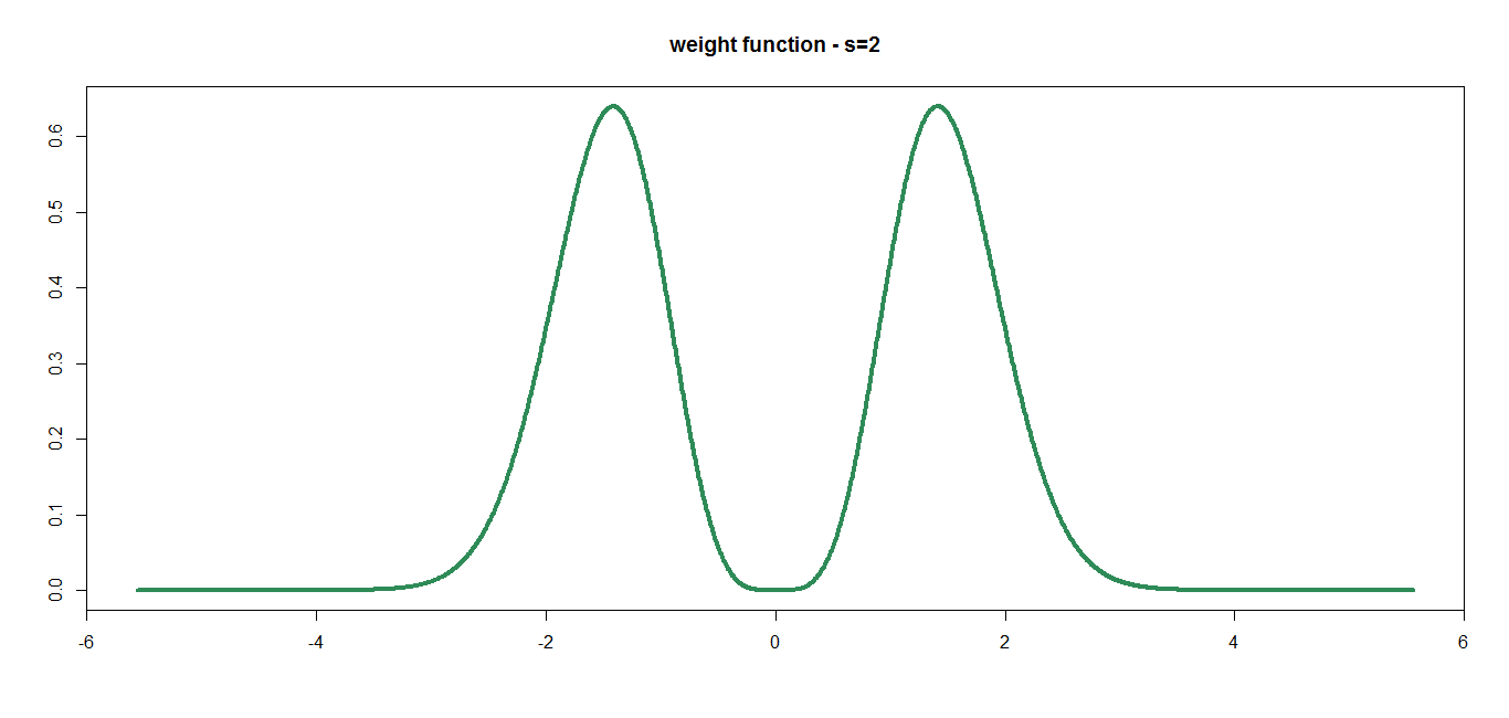
Figure 1: the weight function $w_{s}$ for $s=2$.

Consider now the function $w_{s}:\mathbb{R}\rightarrow\mathbb{R}_{+}$, named weight function (cfr. Figure 1) and defined as

$$w_{s}\left(x\right):=x^{s}\exp\left(-x\right)\text{ , }x\in\mathbb{R}\text{ .}$$ (3)

Following [20], from the Calderon formula and for $t\in\mathbb{R}_{+}$, we define

$$e_{s}:=\int_{0}^{\infty}\left|w_{s}\left(tx\right)\right|^{2}\frac{dx}{x}=\frac{\Gamma\left(2s\right)}{2^{2s}}\text{ ;}$$

on the other hand, (see [22]) fixing the scale parameter $B>1$, from the Daubechies’ Condition it follows that

$$\Lambda_{B,s}m_{B}\leq\sum_{j=-\infty}^{\infty}\left|w_{s}\left(tB^{-2j}\right)\right|^{2}\leq\Lambda_{B,s}M_{B}\text{ ,}$$

where $\Lambda_{B,s}=e_{s}\left(2\log B\right)^{-1}$, $M_{B}=\left(1+O_{B}\left(\left|B-1\right|^{2}\log\left|B-1\right|\right)\right)$ and $m_{B}=\left(1-O_{B}\left(\left|B-1\right|^{2}\log\left|B-1\right|\right)\right)$.

Fixed the resolution level $j\in\mathbb{Z}$, consider a partition of $\mathbb{S}^{1}$ $\left\{E_{jq}:q=1,...,Q_{j}\right\}$ such that for any $q_{1}\neq q_{2}$, $E_{jq_{1}}\cap E_{jq_{2}}=\varnothing$. The region $E_{jk}$ can be described in terms of the couple $\left(\lambda_{jq},x_{jq}\right)$: the positive constant $\lambda_{jq}:=\rho\left(E_{jq}\right)$ is the length of $E_{jq}$, and $x_{jq}\in E_{jq}$ is a generic point belonging to $E_{jq}$. For the sake of simplicity, from now on we will consider $x_{jq}$ as the midpoint of the segment of arc $E_{jq}$. Fixing the shape and the scale parameters $s\in\mathbb{N}$ and $B>1$ (cfr. Figure 2), the circular Mexican needlet $\psi_{jq;s}:\mathbb{S}^{1}\mapsto\mathbb{C}$ is defined as

$$\psi_{jq;s}\left(\theta\right) : =\sqrt{\lambda_{jq}}\sum_{k=-\infty}^{\infty}w_{s}\left(\left(B^{-j}k\right)^{2}\right)\overline{u_{k}\left(x_{jq}\right)}u_{k}\left(\theta\right)$$ (4)

$$= \sqrt{\lambda_{jq}}\sum_{k=-\infty}^{\infty}w_{s}\left(\left(B^{-j}k\right)^{2}\right)\exp\left(ik\left(\theta-x_{ju}\right)\right)\text{, }\theta\in\mathbb{S}^{1}\text{ .}$$

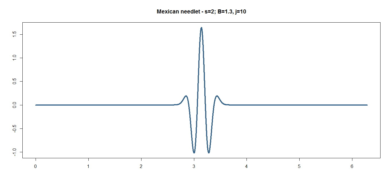
Figure 2: the Mexican needlet corresponding to $s=2$, $j=10$ and $B=1.3$.

For any $F\in$ $L^{2}\left(\mathbb{S}^{1}\right)$, the needlet coefficient $\beta_{jq;s}\in\mathbb{C}$ associated to $\psi_{jq;s}$ is given by

$$\beta_{jq;s}:=\left\langle F,\psi_{jq;s}\right\rangle_{L^{2}\left(\mathbb{S}^{1}\right)}\text{ .}$$ (5)

The system $\left\{\psi_{jq;s}\right\}$, under some regularity conditions, describes a nearly-tight frame over $\mathbb{S}^{1}$, as proved by the Theorem 1.1 in [22] (for general manifold). A set of functions $\left\{g_{i},i\geq 1\right\}$ over a manifold $M$ is said a frame if there exist two positive constant $c_{1}$ and $c_{2}$ (the tightness constants) such that for any $F\in L^{2}\left(M\right)$

$$c_{1}\left\|F\right\|_{L^{2}\left(M\right)}^{2}\leq\sum_{i}\left|\left\langle F,x_{i}\right\rangle_{L^{2}\left(M\right)}\right|^{2}\leq c_{2}\left\|F\right\|_{L^{2}\left(M\right)}^{2}\text{ .}$$

The frame is tight if $c=c_{1}=c_{2}$. If the frame is tight, it is characterized by a reconstruction formula, i.e. for any$F\in L^{2}\left(M\right)$, the following equality holds in the $L^{2}$-sense:

$$F=\frac{1}{\sqrt{c}}\sum_{i}\left\langle F,x_{i}\right\rangle_{L^{2}}x_{i}\text{ ,}$$

which can be roughly viewed as the counterpart of the harmonic expansion in the wavelet framework. As example, we recall that the standard spherical needlets describe a tight frame over the $d$-dimensional sphere $\mathbb{S}^{d}$, cfr. [33, 34]; a frame is nearly-tight if $c_{2}/c_{1}\simeq 1+\varepsilon$, $\varepsilon$ sufficiently close to $0$. In this case, a reconstruction formula does not hold anymore, but it is possible to build a summation formula, such that

$$F=\frac{1}{\sqrt{c}}\sum_{i}\left\langle F,x_{i}\right\rangle_{L^{2}}x_{i}+B_{\epsilon}\text{ .}$$

The bias $B_{\epsilon}$ is smaller as $\epsilon$ is closer to $0$, cfr. [18]. Following Theorem 1.1 in [22], we have that, fixing $B>1$ and $c_{0},\delta_{0}>0$ sufficiently small, there exists a constant $C_{0}$ as follows: (i) for the pixel parameter $\eta\in\left(0,1\right)$ and for $j\in\mathbb{Z}$, there exists a set of measurable sets $\left\{E_{jq},q=1,...,Q_{j}\right\}$, with $\lambda_{jq}\leq\eta B^{-j}$ and for each $j$ with $\eta B^{-j}<\delta_{0}$, $\lambda_{jq}\geq c_{0}\left(\eta B^{-j}\right)$ for $q=1,...,Q_{j}$; (ii) it holds that

$$\left(\Lambda_{B,s}m_{B}-C_{0}\eta\right)\left\|F\right\|_{L^{2}\left(\mathbb{S}^{1}\right)}^{2}\leq\sum_{j=-\infty}^{\infty}\sum_{q=1}^{Q_{j}}\left|\beta_{jq;s}\right|^{2}\leq\left(\Lambda_{B,s}M_{B}+C_{0}\eta\right)\left\|F\right\|_{L^{2}\left(\mathbb{S}^{1}\right)}^{2}.$$ (6)

If $\left(\Lambda_{B,s}m_{B}-C_{0}\eta\right)>0$, it follows $\left\{\psi_{jq;s}\right\}$ is a nearly tight frame, since

$$\frac{\left(\Lambda_{B,s}M_{B}+C_{0}\eta\right)}{\left(\Lambda_{B,s}m_{B}-C_{0}\eta\right)}\sim\frac{M_{B}}{m_{B}}=1+O_{B}\left(\left|B-1\right|^{2}\log\left|B-1\right|\right)\text{ .}$$

Remark 2.1

Mexican needlets present some remarkable advantages if compared to the standard needlet systems, see for instance [33, 34, 5] and the textbook [31]: first of all, they feature a stronger concentration property in the real domain, cfr. [15, 18, 22]. Then, they do not need an exact system of cubature points and weights but they can be built over a more general partition given by $\left\{E_{jq},q=1,...,Q_{j}\right\}$, cfr. [22]. On the other hand, they present also some disadvantages: spherical needlets are characterized by a compact support in the frequency domain (cfr. [33, 34]), while Mexican needlets are defined over the whole frequency range. Furthermore, as already mentioned, standard needlets describe a tight frame and therefore they enjoy an exact reconstruction formula, which is lacking in the Mexican needlet framework. The former issue is “empirically” compensated by the form of the function $w_{s}$, strongly localized around a dominant term in the frequency domain and very close to zero out of a very limited set of frequencies, substantially equivalent to the compact support of the standard needlets. As far as the latter issue is concerned, the summation formula, the counterpart of the reconstruction formula, is characterized by a bias which is easily controlled by the user given the nearly-tightness of the frame (cfr. [18]).

From now on, we will consider just positive resolution levels $j$. In order to respect the conditions of nearly-tightness, we impose that, for $j>0,$

$$Q_{j}\approx\eta^{-1}B^{j}\text{ , }\lambda_{jq}\approx\eta B^{-j}\text{ .}$$ (7)

The Mexican needlets localization property can be stated as follows: for any $s\in\mathbb{N}$, there exists $c_{s}$ such that

$$\left|\psi_{jk;s}\left(\theta\right)\right|\leq c_{s}B^{\frac{j}{2}}\exp\left(-\left(\frac{B^{j}\left(\theta-x_{jk}\right)}{2}\right)^{2}\right)\left(1+\left(\frac{B^{j}\left(\theta-x_{jk}\right)}{2}\right)^{2s}\right)\text{ ,}$$

cfr. [15, 18, 22]. The localization property leads to very relevant boundedness rules on the $L^{p}$-norms: there exist $\widetilde{c_{p}},\widetilde{C_{p}}>0$ such that

$$\widetilde{c_{p}}B^{j\left(\frac{p}{2}-1\right)}\eta^{\frac{p}{2}}\leq\left\|\psi_{jq;s}\right\|_{L^{p}\left(\mathbb{S}^{1}\right)}^{p}\leq\widetilde{C_{p}}\eta^{\frac{p}{2}}B^{j\left(\frac{p}{2}-1\right)}\text{ ,}$$ (8)

cfr. [15, 18].

2.2 Normal approximations and Stein-Malliavin bounds

This section provides a quick overview on the asymptotic Gaussianity of linear functionals of Poisson random measures, properly adapted to the unit circle $\mathbb{S}^{1}$ and initially introduced in [38, 39]. Here, we follow strictly the analogous findings developed on the sphere $\mathbb{S}^{2}$ in [16]. Further general discussions and more technical details can be found also in [36, 40]. Let us begin this section by introducing some distances between laws of random variables, standard in the literature, which define topologies strictly stronger than the convergence in distribution. While the former, the Wasserstein distance, is used in univariate case, the latter, the $d_{2}$-distance, is exploited in the multivariate case. Let $g\in\mathcal{C}\left(\mathbb{R}^{q}\right)$: its Lipschitz norm is given by

$$\left\|g\right\|_{Lip}=\sup_{x,y\in\mathbb{R}^{q},x\neq y}\frac{\left|g\left(x\right)-g\left(y\right)\right|}{\left\|x-y\right\|_{\mathbb{R}^{q}}}\text{ ;}$$

for $g\in\mathcal{C}^{2}\left(\mathbb{R}^{q}\right)$, let $M_{2}\left(g\right)$ be given by

$$M_{2}\left(g\right)=\sup_{y\in\mathbb{R}^{q}}\left\|Hess\left(g\left(x\right)\right)\right\|_{op}\text{ ,}$$

where $\left\|\cdot\right\|_{op}$ denotes the operator norm.

Definition 2.1

Let $X,Y$ be two random vectors with values on $\mathbb{R}^{q}$, $q\geq 1$, such that $\mathbb{E}\left[\left\|X\right\|_{\mathbb{R}^{q}}\right],$ $\mathbb{E}\left[\left\|Y\right\|_{\mathbb{R}^{q}}\right]<\infty$. The Wasserstein distance $d_{W}$ between the laws of $X~{}$and $Y$ is given by

$$d_{W}\left(X,Y\right)=\sup_{g:\left\|g\right\|_{Lip}\leq 1}\left|\mathbb{E}\left[g\left(X\right)-g\left(Y\right)\right]\right|\text{ .}$$

Definition 2.2

Let $X,Y$ be two random vectors with values on $\mathbb{R}^{q}$, $q\geq 1$, such that $\mathbb{E}\left[\left\|X\right\|_{\mathbb{R}^{q}}\right],$ $\mathbb{E}\left[\left\|Y\right\|_{\mathbb{R}^{q}}\right]<\infty$. The distance $d_{2}$ between the laws of $X~{}$and $Y$ is given by

$$d_{2}\left(X,Y\right)=\sup_{g:\left\|g\right\|_{Lip}\leq 1,M_{2}\left(g\right)\leq 1}\left|\mathbb{E}\left[g\left(X\right)-g\left(Y\right)\right]\right|\text{ .}$$

We recall now the definition of Poisson random measures (cfr. for instance [40]).

Definition 2.3

Let $\left(\Theta,\mathcal{A},\mu\right)$ be a $\sigma$-finite measure space, with no-atomic $\mu$. The collection of random variables $\left\{N\left(A\right):A\in\mathcal{A}\right\}$ taking values on $\mathbb{Z}_{+}\cup\left\{\infty\right\}$ is a Poisson random measure (PRM) on $\Theta$ with control (intensity) measure $\mu$ if the following conditions hold:

1. For every element $A\in\mathcal{A}$, $N\left(A\right)$ has Poisson distribution with parameter $\mu\left(A\right)$;

2. If $A_{1},A_{2},...,A_{n}$ $\in\mathcal{A}$ are pairwise disjoint, then $N\left(A_{1}\right),...,N\left(A_{n}\right)$ are independent.

Remark 2.2

In our case, we choose $\Theta=\mathbb{R}_{+}\times\mathbb{S}^{1}$, with $\mathcal{A}=\mathcal{F}\left(\Theta\right)$, the Borel subsets of $\Theta$; $N$ corresponds to a Poisson random measure on $\Theta$, governed by the intensity $\mu=\tau\times\nu$. As far as $\tau$ is concerned, we have that the map $R_{t}:=\tau\left(\mathds{1}_{\left[0,t\right]}\right)$ is strictly increasing and divergent as $t\rightarrow\infty$ and $\tau\left(\left\{0\right\}\right)=0$. The probability measure on the unit circle $\nu$ is absolutely continuous with respect to the Lebesgue uniform measure, i. e. $\nu\left(d\theta\right)=F\left(\theta\right)\rho\left(d\theta\right)$. From now on, $F$ is bounded away from zero, i.e. there exist two constants $M_{\infty},M_{0}>0$ such that

$$0<M_{0}=\inf_{\theta\in\mathbb{S}^{1}}F\left(\theta\right)\leq F\left(\theta\right)\leq\sup_{\theta\in\mathbb{S}^{1}}\left|F\left(\theta\right)\right|=M_{\infty}<\infty\text{ , }\theta\in\mathbb{S}^{1}\text{.}$$ (9a)

It follows that, for any fixed $$t>0$$, the mapping

$$A\mapsto N_{t}\left(A\right)=:N\left(\mathds{1}_{\left[0,t\right]}\times A\right)\text{ }$$

corresponds to a PRM over $\mathbb{S}^{1}$ with control

$$\mu_{t}\left(d\theta\right)=R_{t}\times\nu\left(d\theta\right)=R_{t}\times F\left(\theta\right)d\theta\text{ ,}$$

cfr. Point (i), Remark 2.4 in [16]. Furthermore, as stated in Point (ii), Remark 2.4 in [16], given $\left\{X_{i},i\geq 1\right\}$, the sequence of i.i.d. random variables on $\mathbb{S}^{1}$ with distribution $\nu$, for any $t>0$, it holds the identity in distribution between the two mappings $A\mapsto N_{t}\left(A\right)$ and $A\mapsto\sum_{i=1}^{N_{t}}\delta_{X_{i}}\left(A\right)$, where $\delta_{\cdot}\left(\cdot\right)$ is the Kronecker delta function and $N_{t}$ is an independent Poisson random variable with intensity $R_{t}$.

For any kernel $f\in L^{2}\left(\Theta,\mu\right)\cap L^{1}\left(\Theta,\mu\right)$, with the notation $N\left(f\right)$ and $\widetilde{N}\left(f\right)$ we will denote respectively the Wiener-Itô integrals with respect to $N$ and the corresponding compensated measure $\widetilde{N}\left(A\right)=N\left(A\right)-\mu\left(A\right)$, $A\in\mathcal{F}\left(\Theta\right)$, with the convention $N\left(A\right)-\mu\left(A\right)=\infty$ whereas $\mu\left(A\right)=\infty$. Furthermore, the following isometry property holds: for every $f,g$ $\in L^{2}\left(\Theta,\mu\right)$,

$$\mathbb{E}\left[\widetilde{N}\left(f\right)\widetilde{N}\left(g\right)\right]=\int_{\Theta}f\left(x\right)g\left(x\right)dx\text{ ,}$$

More details can be found in [40].

Finally, we present to rate of convergence to Gaussianity of Wiener-Itô integrals with respect some compensated measure $\widetilde{N}$ obtained by the combination of the Stein’s method for probabilistic approximations and the Malliavin calculus of variations, involving random variables lying in the first Wiener chaos of $N$. These results are here properly adapted to $\mathbb{S}^{1}$. The first bound, concerning normal approximation in dimension $1$ and the Wasserstein distance, was introduced in [38], while the second one, for the $d$-dimensional case, $d>1$, was introduced in [39].

Proposition 2.1

Let $h\in L^{2}\left(\mathbb{S}^{1},\mu_{t}\right)\cap L^{3}\left(\mathbb{S}^{1},\mu_{t}\right)$, let $Z\sim\mathcal{N}\left(0,1\right)$ and let $t>0$, then the following bound holds

$$d_{W}\left(\widetilde{N}_{t}\left(h\right),Z\right)\leq\left|1-\left\|h\right\|_{L^{2}\left(\mathbb{S}^{1},\mu_{t}\right)}^{2}\right|+\int_{\mathbb{S}^{1}}\left|h\left(\theta\right)\right|^{3}\mu_{t}\left(d\theta\right)\text{ .}$$ (10a)

Therefore, if $$\lim_{t\rightarrow\infty}\left\|h\right\|_{L^{2}\left(\mathbb{S}^{1},\mu_{t}\right)}=1 \lim_{t\rightarrow\infty}\left\|h\right\|_{L^{3}\left(\mathbb{S}^{1},\mu_{t}\right)}=0$$ and , it holds that

$$\widetilde{N}_{t}\left(h\right)\rightarrow_{d}Z\text{ .}$$

For $d>1$, let $Z_{d}\sim\mathcal{N}_{d}\left(0,\mathcal{\Sigma}\right)$, where $\Sigma$ is a $d$-dimensional positive-definite covariance matrix, $h_{1},...,h_{d}\in L^{2}\left(\mathbb{S}^{1},\mu_{t}\right)\cap L^{3}\left(\mathbb{S}^{1},\mu_{t}\right)$; let

$$G_{t}:=\left(\widetilde{N}_{t}\left(h_{1}\right),...,\widetilde{N}_{t}\left(h_{d}\right)\right)\text{ ,}$$

associated to a covariance matrix $\mathcal{C}_{d}$ whose elements are given by

$$\mathcal{C}_{d}\left(i_{1},i_{2}\right)=\mathbb{E}\left[\widetilde{N}_{t}\left(h_{i_{1}}\right)\widetilde{N}_{t}\left(h_{i_{2}}\right)\right]=\left\langle h_{i_{1}},h_{i_{2}}\right\rangle_{L^{2}\left(\mathbb{S}^{1},\mu_{t}\right)}\text{ , }i_{1},i_{2}=1,...,d\text{ .}$$

Hence it holds that

$$d_{2}\left(G_{t},Z_{d}\right) \leq \left\|\Sigma^{-1}\right\|_{op}\left\|\Sigma\right\|_{op}^{\frac{1}{2}}\left\|\Sigma-\mathcal{C}_{d}\right\|_{H.S.}+\frac{\sqrt{2\pi}}{8}\left\|\Sigma^{-1}\right\|_{op}^{\frac{3}{2}}\left\|\Sigma\right\|_{op}$$ (11)

$$\times\sum_{i_{1},i_{2},i_{3}=1}^{d}\int_{\mathbb{S}^{1}}\left|h_{i_{1}}\left(\theta\right)\right|\left|h_{i_{2}}\left(\theta\right)\right|\left|h_{i_{3}}\left(\theta\right)\right|\mu_{t}\left(d\theta\right)\text{ ,}$$

where $\left\|\cdot\right\|_{op}$ and $\left\|\cdot\right\|_{H.S.}$ denote respectively operator and Hilbert-Schmidt norms.

3 Rates of convergence to Gaussianity of Mexican needlet coefficients

In this section will study the asymptotic behaviour of the means of the Mexican needlet coefficients, establishing two quantitative central limit theorems and their explicit rates of convergence. Under the assumptions stated in the previous section, let $\left\{X_{i},i\geq 1\right\}$ be a sequence of i.i.d. random variables with distribution $\nu$, independent of the Poisson process $\widetilde{N_{t}}\left(\mathbb{S}^{1}\right)$. Consider the following kernel

$$h_{jq;s}^{\left(R_{t}\right)}\left(\theta\right):=\frac{\psi_{jq;s}\left(\theta\right)}{\sqrt{R_{t}}\sigma_{jq;s}}\text{ , }\theta\in\mathbb{S}^{1}\text{ ,}$$ (12)

where $h_{jq;s}^{\left(R_{t}\right)}\in L^{1}\left(\mathbb{S}^{1},\mu_{t}\right)\cap L^{2}\left(\mathbb{S}^{1},\mu_{t}\right)\cap L^{3}\left(\mathbb{S}^{1},\mu_{t}\right)$. Let $b_{jq;s}:=\mathbb{E}\left[\psi_{jq;s}\left(X_{1}\right)\right]$ and $\sigma_{jq;s}^{2}:=\mathbb{E}\left[\psi_{jq;s}^{2}\left(X_{1}\right)\right]$. Observe that, using (9a) and (8),

$$0<M_{0}\eta\widetilde{c_{2}}\leq M_{0}\left\|\psi_{jq;s}\right\|_{L^{2}\left(\mathbb{S}^{1}\right)}^{2}\leq\sigma_{jq;s}^{2}\leq M_{\infty}\left\|\psi_{jq;s}\right\|_{L^{2}\left(\mathbb{S}^{1}\right)}^{2}\leq M_{\infty}\eta\widetilde{C_{2}}<\infty$$ (13)

Let us write

$$\widetilde{\beta}_{jq;s}^{\left(R_{t}\right)}:=\widetilde{N_{t}}\left(h_{jq;s}^{\left(R_{t}\right)}\right)=\sum_{\theta\in\mathop{\mathrm{s}upp}\left(N_{t}\right)}h_{jq;s}^{\left(R_{t}\right)}\left(\theta\right)-R_{t}\int_{\mathbb{S}^{1}}h_{jq;s}^{\left(R_{t}\right)}\left(\theta\right)\nu\left(d\theta\right)\text{ ,}$$

or, in view of the Remark 2.2,

$$\widetilde{\beta}_{jq;s}^{\left(R_{t}\right)}=\frac{\sum_{i=1}^{N_{t}\left(\mathbb{S}^{1}\right)}\psi_{jq;s}\left(X_{i}\right)-R_{t}b_{jq;s}}{\sqrt{R_{t}}\sigma_{jq;s}}\text{ ,}$$ (14)

It is immediate to see that $\mathbb{E}\left[\widetilde{\beta}_{jq;s}^{\left(R_{t}\right)}\right]=0$, $\mathbb{E}\left[\left(\widetilde{\beta}_{jq;s}^{\left(R_{t}\right)}\right)^{2}\right]=1$. Let us finally define the $d$-dimensional vector

$$Y_{t}=\left(\widetilde{\beta}_{jq_{1};s}^{\left(R_{t}\right)},...,\widetilde{\beta}_{jq_{d};s}^{\left(R_{t}\right)}\right)\text{ ,}$$ (15)

while each element of its covariance matrix is given by

$$\Upsilon_{t,j,s}\left(q_{i_{1}},q_{i_{2}}\right):=\mathbb{E}\left[\widetilde{\beta}_{jq_{i_{1}};s}^{\left(R_{t}\right)}\widetilde{\beta}_{jq_{i_{2}};s}^{\left(R_{t}\right)}\right]\text{ , }i_{1},i_{2}=1,...,d\text{ .}$$ (16)

Let $Z\sim\mathcal{N}\left(0,I_{d}\right)\,$, where $I_{d}$ is the $d$-dimensional identity matrix. Hence the following results holds.

Theorem 3.1

Let $\widetilde{\beta}_{jq;s}^{\left(R_{t}\right)}$ by given by (14). there exist $C_{0}$ such that

$$d_{W}\left(\widetilde{\beta}_{jq;s}^{\left(R_{t}\right)},Z\right)\leq C_{0}\left(B^{-j}R_{t}\right)^{-\frac{1}{2}}\,\ \text{.}$$

Furthermore, if $\left(B^{-j}R_{t}\right)^{-\frac{1}{2}}=o_{t}\left(1\right)$, we have $\widetilde{\beta}_{jq;s}^{\left(R_{t}\right)}\rightarrow_{d}Z$.

Theorem 3.2

Let $Y_{t}$ by given by (15). there exist $C_{1},C_{2}$ such that

$$d_{2}\left(Y_{t},Z_{d}\right)\leq\widetilde{C_{2}^{\prime}}\exp\left(-B^{2j}\left(x_{jq_{1}}-x_{jq_{2}}\right)^{2}\right)\left(1+B^{2sj}\left(x_{jq_{1}}-x_{jq_{2}}\right)^{2s}\right)+\widetilde{C_{2}^{\prime}}d_{t}\left(B^{-j}R_{t}\right)^{-\frac{1}{2}}\,\ \text{.}$$

Furthermore, if $d_{t}\left(B^{-j}R_{t}\right)^{-\frac{1}{2}}=o_{t}\left(1\right)$, we have $Y_{t}\rightarrow_{d}Z_{d}$.

Observe that in both the cases we have the central limit theorem the Mexican needlet coefficients converge in distribution to the (univariate and multivariate) Gaussian distribution when $B^{j}=B^{j_{t}}=o\left(R_{t}\right)$.

Remark 3.1

Recall that the object $B^{-j}R_{t}$ can viewed as the effective sample size of the Mexican needlet (cfr. Remark 4.3 in [16]). Indeed, $B^{-j}$ can be thought as the ’effective’ scale of the wavelet $\psi_{jq,s}$, i.e. the dimension of the region $E_{jq}$. Hence, we obtain

$$\mathbb{E}\left[\mathop{\mathrm{c}ard}\left\{X_{i}:d\left(X_{i},x_{jq}\right)\leq B^{-j}\right\}\right]\simeq R_{t}\int_{d\left(X_{i},x_{jq}\right)\leq B^{-j}}F\left(\theta\right)d\theta\text{ ,}$$

where

$$M_{0}B^{-j}R_{t}\leq R_{t}\int_{d\left(X_{i},x_{jq}\right)\leq B^{-j}}F\left(\theta\right)d\theta\leq M_{\infty}B^{-j}R_{t}\text{ .}$$

In what follows, before concluding this section, we will prove that the explicit bounds deduced in the Theorems 3.1 and 3.2 can be also extended to the case of linear statistics based on vector of i.i.d. observations rather than on a Poisson measure, by paying the price of an additional factor proportional to $d\left(n\right)n^{-\frac{1}{4}}$. Let us define the de-Poissonized vector

$$Y_{n}^{\prime}=\frac{1}{\sqrt{n}}\left(\frac{\sum_{i=1}^{n}\psi_{j\left(n\right)q_{1};s}\left(X_{i}\right)}{\sigma_{j\left(n\right),q_{1};s}},...,\frac{\sum_{i=1}^{n}\psi_{j\left(n\right)q_{d\left(n\right)};s}\left(X_{i}\right)}{\sigma_{j\left(n\right),q_{d\left(n\right)};s}}\right)\text{ ,}$$

and let us recall the following result from [16] (Lemma 1.1).

Proposition 3.3

Let $R\left(n\right)=n$ and consider $X_{i},i\geq 1$, as random variables uniformly distributed over $\mathbb{S}^{1}$. Then, there exists a constant $M_{dP}>0$ such that for every $n$ and every Lipschitz function $f:\mathbb{R}^{d\left(n\right)}\mapsto\mathbb{R}$, the following inequality holds

$$\left|\mathbb{E}\left[f\left(G_{n}^{\prime}\right)-f\left(G_{n}\right)\right]\right|\leq M_{dP}\left\|f\right\|_{Lip}\frac{d\left(n\right)}{n^{\frac{1}{4}}}\text{.}$$

As consequence, there exists $C_{dP}>0$ such that following upper bound holds

$$d_{2}\left(G_{n},Z_{d\left(n\right)}\right)\leq C_{dP}\left(\left(B^{-j\left(n\right)}n\right)^{-\frac{1}{2}}+\frac{M_{dP}}{n^{\frac{1}{4}}}\right)d\left(n\right)\text{ .}$$

4 Proofs

In this Section we describe extensively the proofs of the Theorems 3.1 and 3.2 and of some auxiliary results.

4.1 Proofs of Theorems 3.1 and 3.2

Here we present the exhaustive proofs of the Theorems 3.1 3.2, obtained by using the explicit kernel (12) in the Proposition 2.1 and exploiting the properties of the Mexican needlets such as (8).

Proof of the Theorem 3.1. Using (12) and (13) in (10a), we have

$$1-\left\|h_{jq;s}^{\left(R_{t}\right)}\right\|_{L^{2}\left(\mathbb{S}^{1},\mu_{t}\right)}^{2}=0\text{ , }$$

while

$$\int_{\mathbb{S}^{1}}\left|h_{jq;s}^{\left(R_{t}\right)}\left(\theta\right)\right|^{3}\mu_{t}\left(d\theta\right) = \int_{\mathbb{S}^{1}}\frac{\left|\psi_{jq;s}\left(\theta\right)\right|^{3}}{R_{t}^{\frac{3}{2}}\sigma_{jq;s}^{3}}\mu_{t}\left(d\theta\right)$$

$$\leq \frac{R_{t}^{-\frac{1}{2}}}{\left(M_{0}\eta\widetilde{c_{2}}\right)^{\frac{3}{2}}}\int_{\mathbb{S}^{1}}\left|\psi_{jq;s}\left(\theta\right)\right|^{3}\nu\left(d\theta\right)$$

$$\leq \frac{R_{t}^{-\frac{1}{2}}M_{\infty}}{\left(M_{0}\eta\widetilde{c_{2}}\right)^{\frac{3}{2}}}\left\|\psi_{jq;s}\left(\theta\right)\right\|_{L^{3}\left(\mathbb{S}^{1}\right)}^{3}$$

$$\leq \frac{\widetilde{C_{3}}M_{\infty}}{\left(M_{0}\widetilde{c_{2}}\right)^{\frac{3}{2}}}\left(R_{t}B^{-j}\right)^{-\frac{1}{2}}\text{ ,}$$

where in the last equality we have used (8).   

As far as the multivariate case is concerned, we obtain the following results.

Proof of the Theorem 3.2. By definition, we have

$$\left\|I_{d}^{-1}\right\|_{op}=\left\|I_{d}\right\|_{op}^{\frac{1}{2}}=1\text{ ,}$$

while, following the Lemma 4.1, it holds that

$$\left\|I_{d}-\Upsilon_{t,j,s}\right\|_{H.S.}$$

$$\leq \sqrt{\sum_{q_{1}=q_{2}}\mathbb{E}\left[\widetilde{\beta}_{jq_{1};s}^{\left(R_{t}\right)}\widetilde{\beta}_{jq_{2};s}^{\left(R_{t}\right)}\right]}$$

$$\leq d\sup_{q_{1}\neq q_{2}=1,...,d}\frac{M_{\infty}}{M_{0}\widetilde{c_{2}}}e^{\left(-B^{2j}\left(x_{jq_{1}}-x_{jq_{2}}\right)^{2}\right)}\left(1+\left(B^{j}\left(x_{jq_{1}}-x_{jq_{2}}\right)\right)^{2s}\right)\text{ .}$$

On the other hand, the Lemma 4.2 states that there exists $\widetilde{C}>0$ such that

$$\sum_{i_{1},i_{2},i_{3}=1}^{d}\int_{\mathbb{S}^{1}}\left|\psi_{jq_{i_{1}};s}\left(\theta\right)\right|\left|\psi_{jq_{i_{2}};s}\left(\theta\right)\right|\left|\psi_{jq_{i_{3}};s}\left(\theta\right)\right|\mu_{t}\left(d\theta\right)\leq\widetilde{C}R_{t}dB^{\frac{j}{2}}\text{ .}$$

Hence, we have that

$$\sum_{i_{1},i_{2},i_{3}=1}^{d}\int_{\mathbb{S}^{1}}\left|h_{jq_{i_{1}};s}^{\left(R_{t}\right)}\left(\theta\right)\right|\left|h_{jq_{i_{2}};s}^{\left(R_{t}\right)}\left(\theta\right)\right|\left|h_{jq_{i_{3}};s}^{\left(R_{t}\right)}\left(\theta\right)\right|\mu_{t}\left(d\theta\right)$$

$$\leq\frac{R_{t}^{-\frac{3}{2}}}{\left(M_{0}\eta\widetilde{c_{2}}\right)^{\frac{3}{2}}}\sum_{i_{1},i_{2},i_{3}=1}^{d}\int_{\mathbb{S}^{1}}\left|\psi_{jq_{i_{1}};s}\left(\theta\right)\right|\left|\psi_{jq_{i_{2}};s}\left(\theta\right)\right|\left|\psi_{jq_{i_{3}};s}\left(\theta\right)\right|\mu_{t}\left(d\theta\right)$$

$$\leq\frac{d_{t}\left(R_{t}B^{-j}\right)^{-\frac{1}{2}}\widetilde{C}M_{\infty}}{\left(M_{0}\widetilde{c_{2}}\right)^{\frac{3}{2}}}\text{ ,}$$

as claimed.   

Remark 4.1

As far as the dimension $d$ is concerned, the bound proposed in the Theorem 3.2 holds both if $d$ is fixed and if $d=d_{t}$ grows with $t$, see also [16]. In the former case, the bound obtained depends only on $\left(B^{-j_{t}}R_{t}\right)^{-\frac{1}{2}}$, while in the latter we obtain

$$d_{w}\left(\widetilde{\beta}_{jq;s}^{\left(R_{t}\right)},Z\right)\leq Cd_{t}\left(B^{-j_{t}}R_{t}\right)^{-\frac{1}{2}}\text{.}$$

To attain the convergence in distribution, it suffices that $d_{t}=o_{t}\left(B^{-j_{t}}R_{t}\right)^{-\frac{1}{2}}$

4.2 Auxiliary results

This subsection includes the proofs of the auxiliary Lemmas, mainly related to asymptotic behaviour of the covariance matrix given in (16)

Lemma 4.1

For any $j>0$ and $1\leq q_{1}\neq q_{2}\leq Q_{j^{\prime}}$, there exists a constant $C_{\xi}>0$ such that

$$\left|\mathbb{E}\left[\left|\widetilde{\beta}_{jq_{1};s}^{\left(R_{t}\right)}\widetilde{\beta}_{jq_{2};s}^{\left(R_{t}\right)}\right|\right]\right|\leq C_{\xi}\exp\left(-B^{2j}\left(x_{jq_{1}}-x_{jq_{2}}\right)^{2}\right)\left(1+\left(B^{j}\left(x_{jq_{1}}-x_{jq_{2}}\right)\right)^{2s}\right)\text{ .}$$

Proof. We have that

$$\left|\mathbb{E}\left[\left|\widetilde{\beta}_{jq_{1};s}^{\left(R_{t}\right)}\widetilde{\beta}_{jq_{2};s}^{\left(R_{t}\right)}\right|\right]\right| = \left|\frac{1}{R_{t}\sigma_{jq_{1};s}\sigma_{jq_{2};s}}\int_{\mathbb{S}^{1}}\psi_{jq_{1};s}\left(\theta\right)\psi_{jq_{2};s}\left(\theta\right)\mu_{t}\left(d\theta\right)\right|$$

$$= \frac{1}{\sigma_{jq_{1},s}\sigma_{jq_{2},s}}\left|\int_{\mathbb{S}^{1}}\psi_{jq_{1};s}\left(\theta\right)\psi_{jq_{2};s}\left(\theta\right)F\left(\theta\right)d\theta\right|$$

$$\leq \frac{M_{\infty}}{\eta M_{0}\widetilde{c_{2}}}\left\langle\left|\psi_{jq_{1};s}\right|,\left|\psi_{jq_{2};s}\right|\right\rangle_{L^{2}\left(\mathbb{S}^{1}\right)}\text{ .}$$

Analogously to [16], we split $\mathbb{S}^{1}$ into two regions:

$$S_{1} = \left\{\theta\in\mathbb{S}^{1}:\left(\theta-x_{jq_{1}}\right)^{2}>\left(x_{jq_{1}}-x_{jq_{2}}\right)^{2}/2\right\}$$

$$S_{2} = \left\{\theta\in\mathbb{S}^{1}:\left(\theta-x_{jq_{2}}\right)^{2}>\left(x_{jq_{1}}-x_{jq_{2}}\right)^{2}/2\right\}\text{ .}$$

so that.

$$\left\langle\left|\psi_{jq_{1};s}\right|,\left|\psi_{jq_{2};s}\right|\right\rangle_{L^{2}\left(\mathbb{S}^{1}\right)}\leq\int_{S_{1}}\left|\psi_{jq_{1};s}\left(\theta\right)\psi_{jq_{2};s}\left(\theta\right)\right|d\theta+\int_{S_{2}}\left|\psi_{jq_{1};s}\left(\theta\right)\psi_{jq_{2};s}\left(\theta\right)\right|d\theta$$

From the localization property, it follows that

$$\int_{S_{1}}\left|\psi_{jq_{1};s}\left(\theta\right)\psi_{jq_{2};s}\left(\theta\right)\right|d\theta$$

$$\leq c_{s}^{2}\eta\int_{S_{1}}\exp\left(-B^{2j}\left(\left(\theta-x_{jq_{1}}\right)^{2}+\left(\theta-x_{jq_{2}}\right)^{2}\right)\right)$$

$$\times\left(1+\left(\frac{B^{2j}\left(\theta-x_{jq_{1}}\right)^{2}}{2}\right)^{s}\right)\left(1+\left(\frac{B^{2j}\left(\theta-x_{jq_{2}}\right)^{2}}{2}\right)^{s}\right)B^{j}d\theta$$

$$\leq c_{s}^{2}\eta\exp\left(-B^{2j}\left(x_{jq_{1}}-x_{jq_{2}}\right)^{2}\right)\int_{S_{1}}\exp\left(-B^{2j}\left(\theta-x_{jq_{2}}\right)^{2}\right)$$

$$\times\left(1+\left(\frac{B^{2j}\left(\theta-x_{jq_{1}}\right)^{2}}{2}\right)^{s}\right)\left(1+\left(\frac{B^{2j}\left(\theta-x_{jq_{1}}+x_{jq_{1}}-x_{jq_{2}}\right)^{2}}{2}\right)^{s}\right)B^{j}d\theta$$

$$\leq \left(c_{s}^{\prime}\right)^{2}\eta\exp\left(-B^{2j}\left(x_{jq_{1}}-x_{jq_{2}}\right)^{2}\right)\left(1+B^{2j}\left(x_{jq_{1}}-x_{jq_{2}}\right)^{2s}\right)$$

$$\int_{S_{1}}\exp\left(-B^{2j}\left(\theta-x_{jq_{2}}\right)^{2}\right)\left(1+\left(B^{2j}\left(\theta-x_{jq_{1}}\right)^{2}\right)^{s}\right)^{2}B^{j}d\theta\text{ .}$$

It is immediate to see

$$\int_{S_{1}}\exp\left(-B^{2j}\left(\theta-x_{jq_{2}}\right)^{2}\right)\left(1+\left(B^{2j}\left(\theta-x_{jq_{1}}\right)^{2}\right)^{s}\right)^{2}B^{j}d\theta$$

$$\leq\int_{0}^{\infty}\exp\left(-u^{2}\right)\left(1+u^{2s}\right)^{2}du$$

$$\leq\frac{1}{2}\left(\sqrt{\pi}+2\Gamma\left(s+\frac{1}{2}\right)+2\Gamma\left(2s+\frac{1}{2}\right)\right)\text{ ,}$$

so that

$$\int_{S_{1}}\left|\psi_{jq_{1};s}\left(\theta\right)\psi_{jq_{2};s}\left(\theta\right)\right|d\theta\leq\left(c_{s}^{\prime\prime}\right)^{2}\eta\exp\left(-B^{2j}\left(x_{jq_{1}}-x_{jq_{2}}\right)^{2}\right)\left(1+B^{2sj}\left(x_{jq_{1}}-x_{jq_{2}}\right)^{2s}\right)\text{ .}$$

This concludes the proof.   

Remark 4.2

For $j$ sufficiently large and for $\theta\neq x_{jq}$, there exist $\tau>s$ and $C_{\tau}>0$ such that

$$\frac{\left(1+\left(\frac{B^{j}\left(\theta-x_{jq}\right)}{2}\right)^{2s}\right)}{\exp\left(-\left(\frac{B^{j}\left(\theta-x_{jq}\right)}{2}\right)^{2}\right)}\leq C_{\tau}\left(1+\left(\frac{B^{j}\left(\theta-x_{jq}\right)}{2}\right)\right)^{-\tau}$$

Lemma 4.2

Let $\psi_{jq;s}\left(\cdot\right)$ be given by (4). For $j\geq 1$, there exists $C>0$ such that

$$\sum_{q_{1},q_{2},q_{3}=1}^{d}\int_{\mathbb{S}^{1}}\left|\psi_{jq_{1};s}\left(\theta\right)\right|\left|\psi_{jq_{2};s}\left(\theta\right)\right|\left|\psi_{jq_{3};s}\left(\theta\right)\right|d\theta\leq Cd\eta^{\frac{3}{2}}B^{\frac{j}{2}}\text{ .}$$

Proof. Let $\Im\left(\theta_{0},r\right)$ the arc centered on $\theta_{0}$ of length $r$. Hence, for any $\theta\in\Im\left(x_{jm},B^{-j}\right)$

$$\sum_{q_{1},q_{2},q_{3}=1}^{d}\int_{\mathbb{S}^{1}}\left|\psi_{jq_{1};s}\left(\theta\right)\right|\left|\psi_{jq_{2};s}\left(\theta\right)\right|\left|\psi_{jq_{3};s}\left(\theta\right)\right|d\theta$$

$$\leq\sum_{m}\int_{\Im\left(x_{j^{\prime}m},B^{-j}\right)}\left(\sum_{q=1}^{d}\left|\psi_{jq;s}\left(\theta\right)\right|\right)^{3}d\theta\text{ .}$$

Observe that

$$\sum_{q=1}^{d}\left|\psi_{jq;s}\left(\theta\right)\right|$$

$$\leq c_{s}\eta^{\frac{1}{2}}B^{\frac{j}{2}}\sum_{q=1}^{d}\exp\left(-\left(\frac{B^{j}\left(\theta-x_{jq}\right)}{2}\right)^{2}\right)\left(1+\left(\frac{B^{j}\left(\theta-x_{jq}\right)}{2}\right)^{2s}\right)$$

$$\leq c_{s}\eta^{\frac{1}{2}}B^{\frac{j}{2}}+c_{s}\eta B^{\frac{j}{2}}\sum_{q:=x_{jk}\notin\Im\left(x_{jm},B^{-j}\right)}^{d}\exp\left(-\left(\frac{B^{j}\left(\theta-x_{jq}\right)}{2}\right)^{2}\right)$$

$$\times\left(1+\left(\frac{B^{j}\left(\theta-x_{jq}\right)}{2}\right)^{2s}\right)\text{ .}$$

Now, in view of Remark 4.2, there exists $\tau>s$ such that

$$\sum_{q:=x_{jq}\notin\Im\left(x_{jm},B^{-j}\right)}^{d}B^{\frac{j}{2}}\exp\left(-\left(\frac{B^{j}\left(\theta-x_{jq}\right)}{2}\right)^{2}\right)\left(1+\left(\frac{B^{j}\left(\theta-x_{jq}\right)}{2}\right)^{2s}\right)$$

$$\leq c_{\tau}\sum_{q:=x_{jq}\notin\Im\left(x_{jm},B^{-j}\right)}^{d}B^{\frac{j}{2}}\left(1+\left(B^{2j}\left(\theta-x_{jq}\right)^{2}\right)\right)^{-\tau}\text{ .}$$

As in [16], by using triangle inequality, for $x_{jq}\notin\Im\left(x_{jm},B^{-j}\right),$ $\theta\in\Im\left(x_{jq},B^{-j}\right)$

$$\left(x_{jq}-x_{jm}\right)^{2}+\left(\theta-x_{jq}\right)^{2}\geq\left(\theta-x_{jm}\right)^{2}\text{ ,}$$

we have

$$\sum_{q:=x_{jq}\notin\Im\left(x_{jm},B^{-j}\right)}B^{\frac{j}{2}}\left(1+\left(B^{2j}\left(\theta-x_{jq}\right)^{2}\right)\right)^{-\tau}$$

$$\leq \sum_{q:=x_{jq}\notin\Im\left(x_{jm},B^{-j}\right)}B^{\frac{j}{2}}\left(B^{2j}\left(x_{jm}-x_{jq}\right)^{2}\right)^{-\tau}$$

$$\leq \sum_{q:=x_{jq}\notin\Im\left(x_{jm},B^{-j}\right)}\frac{c_{\tau}^{\prime}}{\rho\left(\Im\left(x_{jm},B^{-j}\right)\right)}\int_{\Im\left(x_{jm},B^{-j}\right)}B^{\frac{j}{2}}\left(B^{2j}\left(x_{jm}-x_{jq}\right)^{2}\right)^{-\tau}dx$$

$$\leq \sum_{q:=x_{jq}\notin\Im\left(x_{jm},B^{-j}\right)}\frac{c_{\tau}^{\prime}}{\rho\left(\Im\left(x_{jm},B^{-j}\right)\right)}\int_{\Im\left(x_{jm},B^{-j}\right)}2^{\tau}B^{\frac{j}{2}}\left(B^{2j}\left(x_{jm}-x\right)^{2}\right)^{-\tau}dx$$

$$\leq c_{\tau}^{\prime\prime}B^{\frac{j}{2}}\text{ ,}$$

as in [16], Theorem 5.5. Therefore we have

$$\sum_{q=1}^{d}\left|\psi_{jq;s}\left(\theta\right)\right|\leq C_{\tau}\eta^{\frac{1}{2}}B^{\frac{j}{2}}\text{ ,}$$ (17)

which leads to

$$\sum_{m}\int_{\Im\left(x_{jm},B^{-j^{\prime}}\right)}\left(\sum_{q=1}^{d}\left|\psi_{jq;s}\left(\theta\right)\right|\right)^{3}d\theta\leq\widetilde{C_{\tau}}\eta^{\frac{3}{2}}B^{\frac{3}{2}j}\text{ .}$$

To complete the proof, we use (17) to have

$$\int_{\mathbb{S}^{1}}\left(\sum_{q=1}^{d}\left|\psi_{jq;s}\left(\theta\right)\right|\right)^{3}d\theta = \sum_{q_{1}=1}^{d}\int_{\mathbb{S}^{1}}\left|\psi_{jq_{1};s}\left(\theta\right)\right|\sum_{q_{2}=1}^{d}\left|\psi_{jq;s}\left(\theta\right)\right|\sum_{q_{3}=1}^{d}\left|\psi_{jq_{3};s}\left(\theta\right)\right|d\theta$$

$$\leq C_{\tau}^{2}\eta B^{j}\sum_{q_{1}=1}^{d}\int_{\mathbb{S}^{1}}\left|\psi_{jq_{1};s}\left(\theta\right)\right|d\theta$$

$$\leq C_{\tau}^{2}\eta B^{j}\sum_{q_{1}=1}^{d}\left\|\psi_{jq_{1};s}\right\|_{L^{1}\left(\mathbb{S}^{1}\right)}$$

$$\leq C_{\tau}^{2}d\eta^{\frac{3}{2}}B^{\frac{j}{2}}\text{ .}$$

 

5 An application: nonparametric density estimation

In this section, we will present a practical application in the framework of nonparametric thresholding density estimation. The thresholding techniques, introduced in the literature by [11], have become a successful tool in statistics, used in many research fields, cfr. the textbooks [25, 45]. The asymptotic result here established are related to random vectors on the unit circle assuming the form (in the “de-Poissonized” case)

$$\widehat{\beta}_{jq;s}^{\left(n\right)}=\frac{1}{n}\sum_{i=1}^{n}\psi_{jq;s}\left(X_{i}\right)\text{ . }$$

Consider now a set of random circular observations $\left\{X_{i}\in\mathbb{S}^{1}:i=1,...,n\right\}$ with common distribution $v\left(\theta\right)=F\left(\theta\right)d\theta$. Let us introduce the threshold $\zeta_{jq}\left(\tau_{n}\right):=\mathds{1}_{\left\{\left|\beta_{jq;s}\right|\geq\kappa\tau_{n}\right\}}$ , where $\kappa$ is a real-valued positive constant to be chosen to set the size of the threshold (cfr. [5, 18]): the thresholding density estimator is given by

$$\widehat{F}\left(\theta\right)=\sum_{j=J_{0}}^{J_{n}}\sum_{q=1}^{Q_{j}}\zeta_{jq}\left(\tau_{n}\right)\widehat{\beta}_{jq;s}\psi_{jq;s}\left(\theta\right)\text{ , }\theta\in\mathbb{S}^{1}\text{ . }$$ (18)

where $\tau_{n}=\sqrt{\frac{\log n}{n}}$, as usual in the literature (see for instance [5, 12, 18, 25]). Further details on this topic can be found in [18]. Finite-sample approximations on the distribution of the coefficients $\widehat{\beta}_{jq;s}$ can be useful to fix an optimal value of the thresholding constant $\kappa$, by using a plug-in procedure built as follows

1. Fixed  a resolution level $j^{\ast}$, the finite-sample approximations on the distributions of the coefficients $\widehat{\beta}_{j^{\ast}q;s}$ can be establish explicitly their corresponding expected values and variances.

2. Using those informations, an optimal threshold $\kappa\tau_{n}$ can be built.

3. Study the nonparametric density estimator $\widehat{F}$ with the optimal threshold.

More in details, $\tau_{n}$ depends on $R_{t}$, while $\kappa$ can be built on the value of sample expected values and variances. In particular, observe that for the cut-off frequency $J_{n}\equiv J_{R_{t}}$, usually chosen such that $B^{J_{R_{t}}}=\sqrt{R_{t}/\log\left(R_{t}\right)}$, we have that

$$d_{2}\left(\widetilde{\beta}_{jq;s}^{\left(R_{t}\right)},Z\right)\leq O\left(\left(\log\left(R_{t}\right)\right)^{-\frac{1}{2}}\right)\underset{t\rightarrow\infty}{\longrightarrow}0\text{ .}$$

6 Numerical results

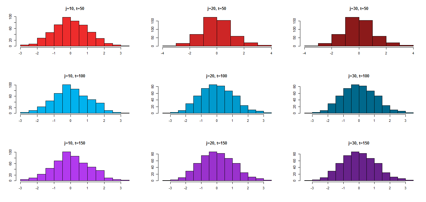
Figure 3: histograms of estimates of Mexican needlet coefficients corresponding to various choices of $j$ and $t$.

In this section we will present some numerical evidences obtained by simulations on CRAN R-code. Observe that these results, obtained in a finite sample situation, can be considered just as a qualitative check of the main theoretical achievements here proposed. We develop a procedure to build Mexican coefficients, in the univariate case, according to the following guidelines:

1. the distribution on $\mathbb{S}^{1}$ is uniform, such that for any $j,q$

   $$b_{jq;s} = 0,$$

   $$\sigma^{2}_{jq;s} = \frac{\Gamma\left(2s+\frac{1}{2}\right)}{2^{\left(2s+\frac{1}{2}\right)}}.$$

2. the intensity of the Poisson process is given by $R_{t}=R\cdot t$, with $R=10$ and $t=50,100,150$.

3. the needlets taken into account corresponds to the resolution levels: $j=10,20,30$, while we fixed $B=1.3$, $x_{jq}=\pi$ and $s=3$.

Shapiro-Wilk test
		$W$	$p$-value
	$j=10$	0.9962	0.28
$t=50$	$j=20$	0.9962	0.28
	$j=30$	0.9960	0.29
	$j=10$	0.9971	0.54
$t=100$	$j=20$	0.9970	0.53
	$j=30$	0.9968	0.52
	$j=10$	0.9981	0.85
$t=150$	$j=20$	0.9983	0.84
	$j=30$	0.9984	0.86

Table 1: Result of the Shapiro-Wilk test.

In Figure 3, each histogram describes the normalized Mexican coefficients built after the iteration of $N_{max}=500$ simulations, combining $j=10,20,30$ and $t=50,100,150$. Observe that they attain fastly the Gaussianity, as confirmed in Table 1 by the results of the Shapiro-Wilk test. Indeed, the test statistic $W$ is closer to $1$ for growing $t$ and it is slowing decreasing as $j$ increases. Furthermore, $p$-values increase strongly with $t$. As a counterexample, in Figure 4 we describe the distribution corresponding to the case $t=5,j=40$, on which the Gaussianity does not seem to be attained, as confirmed by the Shapiro-Wilk which gives as result $W=0.9719,$ $p$-value $=3.207\cdot 10^{-8}$.

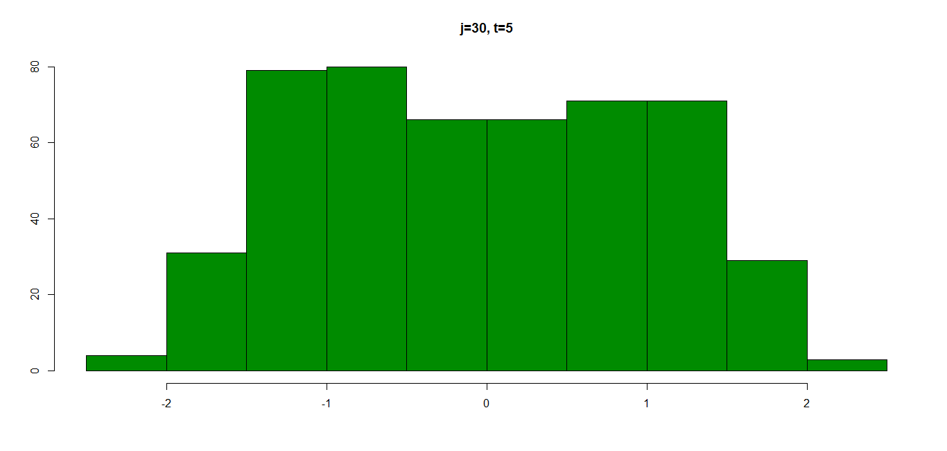
Figure 4: histogram of estimates of Mexican needlet coefficients corresponding to $j=30$ and $t=5$.

Acknowledgements - The author whishes to thank D. Marinucci for the useful discussions and E. Calfa for the accurate reading.

References

- [1] Al-Sharadqah, A., Chernov N., (2009). Error analysis for circle fitting algorithms, Elect. Jour. of Stat, Vol. 3, 886–911.
- [2] Antoine, J.-P. and Vandergheynst, P. (2007), Wavelets on the Sphere and Other Conic Sections, Journal of Fourier Analysis and its Applications,13, 369-386.
- [3] Azmoodeh, E., Campese, S., Poly G. (2013). Fourth Moment Theorems for Markov Diffusion Generators, Journal of Functional Analysis, in press.
- [4] Baldi, P., Kerkyacharian, G., Marinucci, D. and Picard, D. (2009). Asymptotics for Spherical Needlets, Annals of Statistics, Vol. 37, No. 3, 1150-1171.
- [5] Baldi, P., Kerkyacharian, G., Marinucci, D. and Picard, D. (2009) Adaptive Density Estimation for directional Data Using Needlets, Annals of Statistics, Vol. 37, No. 6A, 3362-3395, arXiv: 0807.5059
- [6] Bhattacharya A., Bhattacharya R. (2008), Nonparametric Statistics on Manifolds with Applications to Shape Spaces. In Pushing the Limits of Contemporary Statistics: Contributions in Honor of J. K. Ghosh, IMS Lecture Series.
- [7] Bourguin, S., Peccati, G. (2012). A portmanteau inequality on the Poisson space, submitted.
- [8] Bourguin, S., Durastanti, C., Marinucci, D., Peccati, G. (2014). Gaussian Approximation of nonlinear statistics on the sphere, submitted.
- [9] Cammarota, V., Marinucci, D. (2013), On the Limiting Behaviour of Needlets Polyspectra, in press.
- [10] Di Marzio, M., Panzera A., Taylor, C.C. (2009). Local polynomial regression for circular predictors. Statistics & Probability Letters, Vol. 79, Is. 19, 2066–2075.
- [11] Donoho, D, Johnstone, I. (1991), Minimax estimation via wavelet shrinkage, Tech. Report, Stanford University.
- [12] Durastanti, C., Geller, D., Marinucci D. (2012), Adaptive nonparametric regression on spin fiber bundles, Journal of Multivariate Analysis 104 (1), 16-38.
- [13] Durastanti, C., Lan, X., Marinucci D. (2013), Needlet-Whittle estimates on the unit sphere, Electron. J. Statist., Volume 7, 597-646.
- [14] Durastanti, C., Lan, X., (2013), High-Frequency Tail Index Estimation by Nearly Tight Frames, AMS Contemporary Mathematics, Vol. 603.
- [15] Durastanti, C. (2013). Tail Behaviour of Mexican Needlets. Submitted.
- [16] Durastanti, C., Marinucci, D., Peccati, G. (2013). Normal Approximations for Wavelet Coefficients on Spherical Poisson Fields. Journal of Mathematical Analysis and its Applications, 409, 1, 212-227.
- [17] Durastanti C. (2015). Block Thresholding on the Sphere, Sankhya A, to appear.
- [18] Durastanti C. (2015). Adaptive Density Estimation on the Circle by Nearly-Tight Frames , submitted.
- [19] Fisher, NI. (1993). Statistical Analysis of Circular Data, Cambridge University Press.
- [20] Geller, D. and Mayeli, A. (2006). Continuous Wavelets and Frames on Stratified Lie Groups I. Journal of Fourier Analysis and Applications, Vol. 12, Is. 5, pp. 543-579.
- [21] Geller, D. and Mayeli, A. (2009), Continuous Wavelets on Manifolds, Math. Z., Vol. 262, pp. 895-927, arXiv: math/0602201.
- [22] Geller, D. and Mayeli, A. (2009) Nearly Tight Frames and Space-Frequency Analysis on Compact Manifolds, Math. Z., Vol, 263 (2009), pp. 235-264, arXiv: 0706.3642.
- [23] Geller, D. and Mayeli, A. (2009) Besov Spaces and Frames on Compact Manifolds, Indiana Univ. Math. J., Vol. 58, pp. 2003-2042, arXiv:0709.2452.
- [24] Gorski, K.M., Hivon, E, Banday, A.J., Wandelt, B.D., Hansen, F.K., Reinecke, M, Bartelman, M. (2005), HEALPix, a Framework for High Resolution Discretization, and Fast Analysis of Data Distributed on the Sphere, Astrophys. J. 622:759-771.
- [25] Hardle, W., Kerkyacharian, G., Picard, D., Tsybakov, A. (1998), Wavelets, Approximation and Statistical Applications. Springer.
- [26] Huang, C., Wang, H., Zhang, L. (2011). Berry-Esseen bounds for kernel estimates of stationary processes. Journal of Statistical Planning and Inference, 141, no. 3, 1290-1296.
- [27] Klemela, J. (2000). Estimation of densities and derivatives of densities with directional data, Journal of Multivariate Analysis 73, 18–40.
- [28] Lan, X. and Marinucci, D. (2009), On the Dependence Structure of Wavelet Coefficients for Spherical Random Fields, Stochastic Processes and their Applications, 119, 3749-3766, arXiv:0805.4154.
- [29] Ledoux M., (2012). Chaos of a markov operator and the fourth moment condition, The Annals of Probability 40, no. 6, 2439–2459.
- [30] Li, Y., Wei, C., Xing, G. (2011). Berry-Esseen bounds for wavelet estimator in a regression model with linear process errors, Statist. Probab. Lett., 81, no. 1, 103-110.
- [31] Marinucci, D. and Peccati, G. (2011) Random Fields on the Sphere. Representation, Limit Theorem and Cosmological Applications, Cambridge University Press.
- [32] Mayeli, A. (2010), Asymptotic Uncorrelation for Mexican Needlets, J. Math. Anal. Appl. Vol. 363, Issue 1, pp. 336-344, arXiv: 0806.3009.
- [33] Narcowich, F.J., Petrushev, P. and Ward, J.D. (2006a) Localized Tight Frames on Spheres, SIAM Journal of Mathematical Analysis Vol. 38, pp. 574–594.
- [34] Narcowich, F.J., Petrushev, P. and Ward, J.D. (2006b) Decomposition of Besov and Triebel-Lizorkin Spaces on the Sphere, Journal of Functional Analysis, Vol. 238, 2, 530–564.
- [35] Nourdin, I., Peccati, G. (2009). Stein’s method on Wiener chaos. Probability Theory Related Fields, 145, no. 1-2, 75-118.
- [36] Nourdin, I., Peccati, G. (2012). Normal Approximations using Malliavin calculus: from Stein’s method to universality. Cambridge University Press.
- [37] Nualart, D., Peccati, G. (2005). Central limit theorems for sequences of multiple stochastic integrals. Annals of Probability, 33, no.1, 177-193.
- [38] Peccati, G., Solé J.-L., Taqqu, M.S., Utzet, F. (2010). Stein’s method and normal apprimation for Poisson functionals. The Annals of Probability, 38 (2), 443-478.
- [39] Peccati, G., Zheng, C. (2010). Multi-dimensional Gaussian fluctuationson the Poisson space. Electronic Journal of Probability 15 (48), 1487-1527.
- [40] Peccati, G., Taqqu, M.S. (2010). Wiener chaos: moments, cumulants and diagrams. Springer-Verlag.
- [41] Rao Jammalamadaka, S., Sengupta, A. (2001). Topics in Circular Statistics. World Scientific.
- [42] Scodeller, S., Rudjord, O. Hansen, F.K., Marinucci, D., Geller, D. and Mayeli, A. (2011), Introducing Mexican needlets for CMB analysis: Issues for practical applications and comparison with standard needlets, Astrophysical Journal, 733, 121.
- [43] Silverman, B.W. (1986). Density Estimation for Statistics and Data Analysis. Chapman & Hall CRC Monographs on Statistics & Applied Probability.
- [44] Stein, E., Weiss, G. (1971), Introduction to Fourier Analysis on Euclidean Spaces, Princeton University Press.
- [45] Tsybakov, A.B. (2009) Introduction to Nonparametric Estimation, Springer, New York.
- [46] Yang, W., Hu, S., Wang, X., Ling, N. (2012). The Berry-Esseen type bound of sample quantiles for strong mixing sequence. Journal of Statistical Planning and Inference, 142, no. 3, 660-672.
- [47] Wu, H. (1997). Optimal exact designs on a circle or a circular arc. Ann. Statist., Vol. 25, 5, 2027-2043.