Run Time Approximation of Non-blocking Service Rates for Streaming Systems

Abstract

Stream processing is a compute paradigm that promises safe and efficient parallelism. Modern big-data problems are often well suited for stream processing’s throughput-oriented nature. Realization of efficient stream processing requires monitoring and optimization of multiple communications links. Most techniques to optimize these links use queueing network models or network flow models, which require some idea of the actual execution rate of each independent compute kernel within the system. What we want to know is how fast can each kernel process data independent of other communicating kernels. This is known as the “service rate” of the kernel within the queueing literature. Current approaches to divining service rates are static. Modern workloads, however, are often dynamic. Shared cloud systems also present applications with highly dynamic execution environments (multiple users, hardware migration, etc.). It is therefore desirable to continuously re-tune an application during run time (online) in response to changing conditions. Our approach enables online service rate monitoring under most conditions, obviating the need for reliance on steady state predictions for what are probably non-steady state phenomena. First, some of the difficulties associated with online service rate determination are examined. Second, the algorithm to approximate the online non-blocking service rate is described. Lastly, the algorithm is implemented within the open source RaftLib framework for validation using a simple microbenchmark as well as two full streaming applications.

I Introduction

Stream processing (or data-flow programming) is a compute paradigm that enables parallel execution of sequentially constructed kernels. This is accomplished by managing the flows of data from one sequentially programmed kernel to the next. Flows of data within the stream processing community are known as “streams.” Queueing behavior naturally arises between two kernels independently executing. Selecting the correct queue capacity (buffer size) is one parameter (of many) that can be critical to the overall performance of the streaming system. Doing so, however, often requires information, such as the service rate of each kernel, not typically available at run time (online). Complicating matters further for online optimization, many analytic methods used to solve for optimal buffer size require an understanding of the underlying service process distribution, not just it’s mean. Both service rate and process distribution can be extremely difficult to determine online without effecting the behavior of the application (i.e., degrading application performance). This paper proposes and demonstrates a heuristic that enables online service rate approximation of each compute kernel within a streaming system. It is also shown that this method imposes minimal impact on the monitored application.

An example of a simple streaming application is shown in Figure 1. The kernel labeled as “A” produces output which is “streamed” to kernel “B” over the communications link labeled “Stream.” These communications links are directed (one way). Strict stream processing semantics dictate that all of the state necessary for each kernel to operate is compartmentalized within that kernel, the only communication allowed utilizes the stream. State compartmentalization and subsequent one-way transmittal of state via streaming comes with increased communications between kernels. Increased communication comes with multiple costs depending on the application: increased latency, decreased throughput, higher energy usage. No matter what the cost function is, minimizing its result often involves optimizing the streams (queues and subsequent buffers) connecting individual compute kernels. The buffers forming the streams of the application can be viewed as a queueing network [1, 14]. It is this network that we want to optimize while the application is executing.

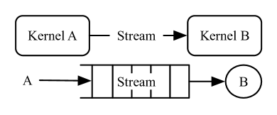
Figure 1: The simple streaming application at top has two compute Kernels A & B with a single stream connecting them. The corresponding queueing network is a single server B with a single queue fed by the arrival process generated by Kernel A.

Optimizing the queueing network that models a streaming application can be performed using analytic techniques. Ubiquitous to many of these models is the non-blocking service rate of each compute kernel. Classic approaches assume a stationary distribution. This carries the assumption that both the workload presented to the compute kernel and its environment are stable over time. One only has to look at the variety of data presented to any common application to realize that the assumption of a persistent homogeneous workload is naive. With the popularity of cloud computing we also have to assume that the environment an application is executing in can change at a moments notice, therefore we must build applications that can be resilient to perturbations in their execution environment. We focus on low overhead instrumentation that will enable more resilient stream processing applications by informing the runtime when conditions change.

When viewing each compute kernel as a “black-box,” as many streaming systems do (e.g., RaftLib [3, 20]), then buffer sizing is one of the most influential knobs available to tune the application aside from resource selection (i.e., the hardware the kernel is executing on). The sizing of each buffer (queue) within a streaming system has very real performance implications (see Figure 2). Too small of a buffer will result in it always being full, stifling performance of upstream compute nodes. On the other hand, bigger buffers are not always better. Extremely large buffers increase the overhead associated with accessing them. Discounting increased allocation time, excessively sized buffers can lead to increased page faults and virtual memory usage which can decrease performance. Large buffers are also wasteful, physical memory is often at a premium, it should be used wisely.

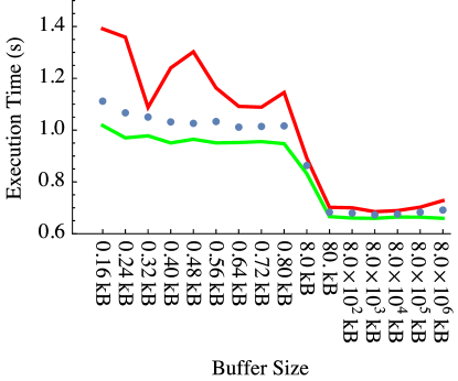
Figure 2: Incorrect buffer sizes can have a deleterious effect on the overall performance of a streaming system. This chart depicts empirical data collected from a matrix multiply application executing on eight threads. The points represent mean execution time, and the lower and upper solid lines are the $5^{th}$ and $95^{th}$ percentiles, respectively. The times are for the overall execution of the algorithm only, no allocation or deallocation time included. The net effect of increased buffer sizes initially improves performance but then slowly degrades as the buffer size is increased.

In addition to being useful for queue (buffer) sizing, service rate observation is also critical for another optimization tasks. Parallelization decisions are often made statically, however streaming systems have the advantage of state compartmentalization. Compartmentalization simplifies parallelization logic, methods such as that described by Gordon et al. [8] or Li et al. [15] can be used at runtime to increase parallelism and improve throughput. Platforms such as RaftLib have the capability of making parallelization decisions both statically and at run-time. One factor to consider when parallelizing a compute kernel is the effective service rate of the kernel itself. Knowledge of the downstream compute kernels’ service rates inform the run-time as to if the system downstream is capable of accepting more input. Knowing the downstream kernel’s non-blocking service rate is exactly what we need to know to make an informed parallelization decision. To the best of our knowledge there have been no other low overhead approaches to determine the online service rate of a compute kernel executing within a streaming system.

In the sections that follow we will first describe some background material and related work, followed by a description of our heuristic approach and it’s implementation within the RaftLib streaming library. The heuristic’s performance is evaluated with hundreds of micro-benchmark executions, and two real world application examples implemented using the RaftLib streaming framework. Finally we will describe how this method can be combined with methods of online moment approximation to potentially estimate the shape of the underlying kernel’s process distribution.

II Background & Related Work

At it’s core, this work is about low-overhead instrumentation of software systems. The same techniques could also be used for co-designed hardware/software systems. Many others have produced low overhead instrumentation systems. Amongst the earliest type of performance oriented instrumentation tools were call graph tools such as gprof [9]. Other instrumentation tools such as TAU [21] provide low overhead instrumentation and visualization for MPI style systems. What these tools don’t provide is a mechanism for reporting performance during execution (which our system does).

Modern stream processing systems such as RaftLib [3, 20] can dynamically re-optimize in response to changing conditions (workload and/or computing environment). To re-optimize buffer allocations there are generally two choices, either branch and bound search or analytic queueing model. Branch and bound search has the disadvantage of requiring multiple allocations and re-allocations until a semi-optimal buffer size is found. Analytic queuing models are highly desirable for this purpose since they can divine a buffer size directly, eschewing many unnecessary buffer re-allocations. Compute kernel mean service rates are, at a minimum, typically required for these types of models. Utilizing these models dynamically therefore requires dynamic instrumentation. Tools such as DTrace [5], Pin [16], and even analysis tools such as Valgrind [18] can provide certain levels of dynamic information on executing threads. Our approaches differ from the aforementioned ones in that we are specifically targeting methods for estimating online service rate in a low overhead manner.

Optimization of the queueing network inherent in stream processing systems through optimal buffer sizing is only one use of online service rate estimation, parallelization control can benefit as well. Parallelization decisions on streaming systems currently suffer from a lack of dynamic knowledge, that is, there really isn’t a way of knowing how parallelizing a kernel will effect the overall performance of an application. When combined with methods described by Beard and Chamberlain [1], knowledge of online service rates can quickly inform the run-time of how duplication will effect the overall application’s throughput.

Work by Lancaster et al. [13] laid out logic that could ostensibly make online service rate determination possible. They suggest measuring the throughput into a kernel when there is sufficient data available within it’s input queue(s) and no back-pressure from its output queue(s). This logic works well for FPGA-based systems where hardware is controlled by the developer. For multi-core systems, however, this logic breaks down, for several reasons which are enumerated within this section. The need for low overhead online service rate determination motivates this work.

The work of Lancaster et al. assumes that the measurements of a non-blocked service rate are all equal (i.e., the full service rate is observed at every sample point). In reality things like partially full queues result in less than realized service rates using this procedure. Further testing reveals that anomalies such as cache behavior and clock variations can further exacerbate understanding of the true service rate of a compute kernel. Making things worse still are context swaps that occur when one independent thread is observing another. In reality, sampling the service rate of a compute kernel looks like Figure 3 where multiple outliers and noise confound our understanding of the true service rate.

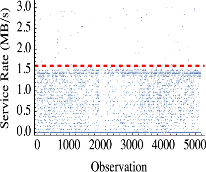
Figure 3: Direct observations of the service rate, using the logic of [13], for a nominally fixed rate microbenchmark kernel. The x-axis is the increasing observation index with time, the y-axis represents the actual data rate observed at each sample point. The red dashed line is the expected service rate as set experimentally.

Central to accurate estimation of service rate is observing non-blocking reads and writes performed by the server. While executing, the probability of observing a non-blocked read or write to a queue in general is very low for high performance systems (i.e., those systems whose compute kernels have high utilization). Equation 1 (a modification of the equations given by Kleinrock [12]) gives these probabilities for the simplified case where each server’s process is Poisson and only a single in-bound queue and out-bound queue are considered (also known as an $M/M/1$ queue, using Kendall’s notation [11]). Equation LABEL:eq:probread is fairly intuitive: with $k=\lceil\mu_{s}T\rceil$, $k$ is the mean number of items to be consumed by the server, what is the probability of $n\geq k$ items existing in the in-bound queue given the service rate of the server ($\mu_{s}$) and the time period ($T$) over which the transactions are observed? Just as intuitive is the estimate for the out-bound queue: for the server to have a non-blocking writes over the entire time period $T$ then the queue must have space for that entire time period, with $k=C-\lceil\mu_{s}T\rceil+1$ and $k$ is the space required by the server’s output, the probability that $n<k$ (here, $n$ is the number of items in the out-bound queue) is given by Equation 1d. Table I gives the list variable definitions. Figure 4 shows this graphically for a selection of throughput rates. In general the shorter the service time, the lower the probability of observing a non-blocking read or write. Lengthening the observation period, $T$, decreases the probability that blocking will not occur during the observation period whereas shorter periods increase the probability of observation (i.e., no blocking during the period).

TABLE I: Nomenclature used for Equation 1

Symbol	Description
$\mu_{s}$	mean service rate
$\rho$	server utilization
$C$	capacity of output queue
$T$	sampling period of monitor
$k$	items needed by server during $T$

$$k=\lceil\mu_{s}T\rceil$$ (1a)

$$Pr_{\mbox{\sc{\small{read}}}}(T,\rho,\mu_{s})=\rho^{k}$$ (1b)

$$Pr_{\mbox{\sc{\small{write}}}}(T,C,\rho,\mu_{s})=\begin{cases}1-\rho^{C-k+1}&C\geq\mu_{s}T\\ 0&C<\mu_{s}T\end{cases}$$ (1d)

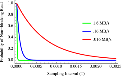
Figure 4: The probability (y-axis) of observing a non-blocking read given the observation period $T$ (x-axis). In general the faster the server or greater throughput the lower the probability of observing a non-blocking read from the queue.

The various mechanics required to estimate an online service rate will be covered in the subsequent sections. We will begin by describing the monitoring system itself at an abstract level, this is followed by setting the observation period and finally the heuristic for online service rate determination itself.

III Monitoring Mechanism

The simple act of observing a rate can change the behavior being observed. This phenomena is more obvious with large real world observations (e.g., observing animal behavior), however it is equally true for micro ones. Data observation might not make the data run away, however each observation requires non-zero perturbation to record it (e.g., a copy from the incremented register at some interval). Alternatively, saving every event under observation can quickly overwhelm the hardware and operating system. Trace files, even when compressed, can grow rapidly. Determining the service rate with trace data in a streaming fashion (saving none of it) might be possible, however it still increases traffic within the memory subsystem which is less than desirable in high performance applications. Concomitant to reducing communications overhead associated with monitoring is moving any computation associated with that instrumentation out of the application’s critical path. To accomplish this, our instrumentation scheme (implemented within RaftLib) uses a separate monitoring thread. This increases the sensitivity to timing precision and the possibility of noise within the observations. Within this section the overall architecture of our implementation is discussed.

At a high level, Figure 5 depicts the arrangement of the instrumentation system under consideration. A simplified streaming application with only two kernels is shown, connected by a single stream. Each kernel is depicted as executing on an independent thread. A monitor (depicted as an eye), performs all the instrumentation work, it executes on an independent thread as well. Each of these threads is scheduled by the streaming run-time and the operating system. Both provide input on when each kernel and the monitor is to execute. Each of these threads also could execute on independent processor cores or a single multiplexed core. Each abstraction layer has the potential to impart noise on any observations made by the monitor, the methods proposed here must deal with and operate in spite of this complexity.

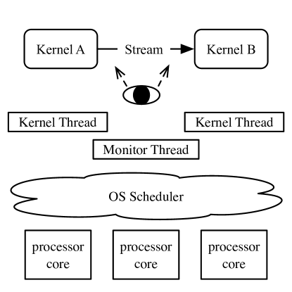
Figure 5: High level depiction of the abstraction layers coalesced around a simple streaming application with two compute kernels. An independent monitor thread serves to instrument the queue. Both the kernel threads and monitor threads are subject to the runtime and operating system (OS) scheduler.

To minimize overall impact, the data necessary to estimate the service rate is split between the queue itself and the monitor thread. This has the benefit of transmitting data only when absolutely necessary. As depicted in Figure 5, the queue itself is now visible to three distinct threads: the monitor thread and the producer/consumer threads at either terminus of the queue. The only logic to consider within the queue itself is that necessary to tell the monitor thread if it has blocked and that necessary to increment a item counter as items are read from or written to the queue. The monitor thread reads these variables written by the run-time controlling the queue (work is actually performed by the producer or consumer threads). The monitor thread also resets or zeros the counter (which will be called $tc$ from this point forward) and blocking boolean kept by the queue. In a non-locking operation, the monitor thread copies and zeros $tc$. This has the advantage of being quite fast, however there are implications.

The monitor thread samples at a fixed interval of time $T$ which is the sampling period. When the monitor thread samples $tc$ and the blocking boolean, it has no way of knowing if the server at either end only performed complete executions or partial ones. The only thing it can be certain of is that the data read are non-blocking if the boolean value is set appropriately. This means that $tc$ can represent something less than the actual service rate. Also contained within the $tc$ are effects not-representative of average behavior; these include (list not exhaustive): caching effects, interrupts, memory contention, faults, etc.

As mentioned previously (see Figure 4), the probability of making a non-blocking observation is in general quite low. In order to improve those odds there are some mechanisms that the run-time can implement. Given a full out-bound queue, resizing the queue provides a brief window over which to observe fully non-blocking behavior. Given an empty in-bound queue there are three implementable actions: (1) increasing the number in-bound servers feeding more arrivals to the queue, (2) changing execution hardware of the up-stream server can have the same effect as the aforementioned approach, (3) adjusting the scheduling frequency before observing full service rate in order to fill the in-bound queue. Our implementation within RaftLib utilizes only the first approach for out-bound queues, future implementations will utilize all of the above further improving service rate determination.

IV Service Rate Monitoring

Online estimation of service rate requires four basic steps: fixing a stable sampling period $T$, sampling only the correct states (expounded upon below), reducing and de-noising the data, then estimating the non-blocking service rate. The queueing system has a finite number of states which are useful in estimating the non-blocking service rate. The most obvious states to ignore are those where the in-bound or out-bound queue is blocked (see Lancaster et al.). As mentioned in Section III there are also data unrepresentative of the non-blocking service rate. Raw data such as Figure 3 are initially collected, filtering this data through the process described below produces a final usable result. We start by describing how we determine a stable sampling period, $T$, followed by the heuristic to process the raw read data, $tc$. Symbols used in this section are summarized in Table II.

TABLE II: Nomenclature used for Section IV

Symbol	Description
$T$	sampling period
$tc$	sum of non-blocking reads during $T$
$S$	windowed set of items $tc$
$S^{\prime}$	Gaussian filtered set of $S$
$q$	$95^{th}$ quantile of $S^{\prime}$
$\bar{q}$	population averaged $q$
$d$	bytes per data item

IV-A Sampling Period Determination

Each queue within a streaming application has it’s own monitor thread. As such, each $T$ is queue specific, since each instrumented queue is in a slightly differing environment. An initial requirement is a stable time reference across all utilized cores. The timing method described by Beard and Chamberlain [2] is employed (our specific implementation uses the x86 rdtsc instruction, but any sufficiently high resolution time reference could be used). This method provides a stable and monotonically increasing time reference whose latency on most systems is approximately $50-300$ ns across the cores. Despite a relatively stable time reference, two trends complicate matters. First, as service time decreases, the probability of observing a non-blocking queue transaction decreases as well (see Equation 1). Second, noise from the system and timing mechanism dominate for very small values of $T$ making observations unusable [4].

Given a common understanding of time across cores, we can now proceed to choose a sampling period, $T$. Modern computing systems (multi-core processors, multiple system services, general purpose operating system, etc.) introduce some level of noise into the measurements [2, 17]. Given that we are measuring service rates, a longer sample period helps to smooth out these disturbances. However, we wish to observe kernel executions that are unimpeaded by their environment (no blocking due to upstream or downstream effects). This pushes us towards a shorter sampling period.

Figure 6 shows how the measured (actual) sampling period varies with desired sampling period, $T$, starting with the minimum latency ($\sim\!300$ ns for this example) of back to back timing requests then iterating over multiples of that latency. The monitor thread tries to find the widest stable time period $T$ (moving to the right in Figure 6) while minimizing observed queue blockage during the period. To make this more concrete, our implementation lengthens the period if: (1) no blockage occurred on the in-bound or out-bound buffer (with respect to a kernel) within the last $k$ periods and (2) the realized period of the monitor was within $\epsilon$ of the current $T$ over the last $j$ periods (i.e., $T$ was stable). Failure to meet these conditions results in the failure of our method (i.e., we conclude that our approach will not result in usable service rate monitoring).

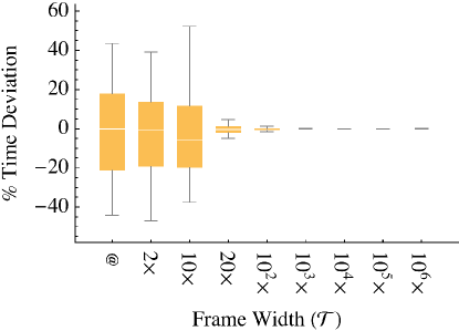
Figure 6: Observations of $T$ variation using the timing mechanism of [2]. The $@$ symbol represents the minimum resolution of the timing mechanism ($\sim\!300$ ns for this example), subsequent box and whisker observations are the indicated multiple of $@$. The trend indicates that wider time frames (up to the approximate time quanta for the scheduler) give more stable values of $T$.

IV-B Service Rate Heuristic

Once a stable $T$ has been determined, the next step is estimating the online service rate without having to store the entire data trace of all queueing transactions. Each queue stores transactional data at each end (referred to as the head and tail). The head and tail of the queue store counts of non-blocking transactions, $tc$, as well as the size of each item copied, $d$. The transaction count, $tc$, requires very little overhead since it is simply a counter. The item size is typically constant for any given queue. The instrumentation thread samples $tc$ from the head and tail of the queue every $T$ seconds. While there are many factors that can slow down a kernel in the context of a full execution, only a few can make it appear to execute faster (see Figure 3). We will use an estimate of the maximum, well-behaved $tc$ to estimate the service rate of interest. (What we mean by well-behaved is articulated below.) For simplicity, the discussion that follows will consider only actions that occur at the head of the queue (departures from the queue into the server), with the understanding that the same actions occur at the tail as well.

The overall process described below is summarized in Algorithm 1. This description presumes there is an implementaion of a streaming mean and standard deviation (see Welford [22] and Chan et al. [6]) through the $updateStats()$, $updateMeanQ()$ and $resetStats()$ methods. Not described explicitly in the algorithm is the convergence methodology described later in the text, which is implemented within the $QConverged()$ function. Padding is not used for the filter, therefore the filter starts at the radius for the filter so that the result of the filter has a width $2\times\text{radius}$ smaller than the data window.

$stream\leftarrow tc$;

$output\leftarrow$ output stream;

$S\leftarrow\{\}$;

while True do

       $tc_{current}\leftarrow pop(stream)$;

       $S^{\prime}\leftarrow\{\}$;

       for  $i\leftarrow gauss_{radius}$, $i<|window|-gauss_{radius}$,$i++$  do

             $val\leftarrow$ Dot( $S[i-gauss_{radius}$;;$i+gauss_{radius}]$,$GaussianFilter$ );

             push( $S^{\prime}$, $val$ );

            

       end for

      $\mu_{S^{\prime}}\leftarrow$Mean($S^{\prime}$);

       $\sigma_{S^{\prime}}\leftarrow$StandardDeviation( $S^{\prime}$);

       $q\leftarrow$NQuantileFunction( $\mu_{S^{\prime}}$, $\sigma_{S^{\prime}}$, $.95$ );

       updateStats( $q$ ); if  QConverged()  then

             push( $output$, getMeanQ() );

             resetStats();

            

       end if

      

end while

Algorithm 1 Service Rate Heuristic

While sampling $tc$, the timing thread creates an ordered list $S$, where items are ordered by entry time (easily implemented as a first-in first-out queue). $S$ is maintained as a sliding window of size $w$. If $S$ is of sufficient size, then it is expected that the distribution of $tc\in S$ tends toward a Gaussian distribution ($\mathcal{N}(\mu_{S},\sigma_{S})$), as it is a list of sums of non-blocking transactions. $S$, however also consists of many data that are not necessarily indicative of the non-blocking service rates. These elements arise from the following conditions: (1) the monitor thread observed only a partial firing of the server (i.e., the server had the capability to remove $j$ items from the queue but only $<j$ items were evident when retrieving $tc$); (2) the monitor thread clears the queue’s current value of $tc$ during a firing (i.e., the counter maintaining $tc$ is non-locking because locking it introduces delay); (3) outlier conditions as discussed in Section II which are not indicative of normal behavior conspire to speed up or slow down (momentarily) the service rate. We use a Gaussian filter to lessen the impact of these effects.

Filters are frequently used in signal processing applications to de-noise data sets. In general, a filter is a convolution between two distributions so that the response is a combination of both functions. The underlying distribution of $S$ without outliers tends towards a Gaussian, therefore a Gaussian discrete filter is used to shape the data in $S$ so that it is sufficiently well-behaved (de-noised) for estimating the maximum. The filtered data make up the set $S^{\prime}$. The exact Gaussian kernel is described by Equation 2, where $x\leftarrow[-2,2]$ is the index with respect to the center. Through experimentation a radius of two was selected as providing the best balance of fast computation and smoothing effect.

$$GaussianFilterKernel(x)\leftarrow\frac{e^{-\frac{x^{2}}{2}}}{\sqrt{2\pi}}$$ (2)

Once filtered, we use the data of $S^{\prime}$ to estimate the maximum. Since we must still account for outliers, rather than explicitly use the sample maximum, we estimate the maximum of the well-behaved counts via the $95^{th}$ quantile of $S^{\prime}$. This is a reasonable approximation given that: once filtered, $S^{\prime}$ even more closely has a Gaussian distribution than $S$ and a quantile is more robust to outliers than the sample maximum. Operationally, we use the sample mean, $\widehat{\mu_{S^{\prime}}}$, and standard deviation, $\widehat{\sigma_{S^{\prime}}}$, to estimate $\mathcal{N}(\mu_{S^{\prime}},\sigma_{S^{\prime}})$, and the quantile is

$$q=\widehat{\mu_{S^{\prime}}}+1.64485~{}\widehat{\sigma_{S^{\prime}}}.$$ (3)

Direct utilization of $q$ is sufficient for some purposes, however it is only valid for the time period comprising the window over which it was collected $p\leftarrow T\times w$. Subsequent sets $S^{\prime}_{i}$ update $\mu_{S^{\prime}}$ and $\sigma_{S^{\prime}}$ resulting in frequent new values (e.g., Figure 7). Stability is gained by using the online mean of successive values of $q_{i}$. Where $\bar{q}$ is the averaged, estimated maximum non-blocking transaction count $tc$, assuming only one queue for simplicity, the service rate is simply $\frac{\bar{q}\times d}{T}$. This, however also assumes that the underlying distribution generating $tc$ is also stable. As with all online estimates, that of $\bar{q}$ becomes more stable with more observations (e.g., Figure 8).

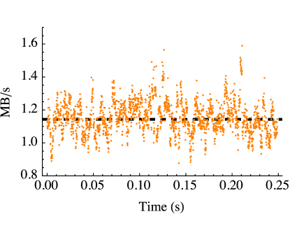
Figure 7: Plot of the values of $q$ with increasing time. Each value of $q$ is the result of a computation of Equation 3. The dashed line across the $y$-axis represents the set or expected service rate.

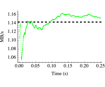
Figure 8: An example of convergence of $\bar{q}$ with increasing time. This data is from a single queue tandem server micro-benchmark, observing the departure rate from the queue to the server with the set service rate marked as a dashed line.

Convergence of $\bar{q}$ to a “stable” value is expected after a sufficiently large number of observations. In practice, with micro-second level sampling, convergence is rarely an issue at steady state. Determining when $\bar{q}$ is stable is accomplished by observing $\sigma$ of $\bar{q}$. Minimizing the standard deviation is equivalent to minimizing the error of $\bar{q}$. With a finite number of samples, it is unlikely that $\sigma(\bar{q})$ will ever equal to zero, however observing the rate of change of the error term to a given tolerance close to zero is a typical approach. A similar windowed approach as that taken above is used, however with differing filters to approximate the relative change over the window. A discrete Gaussian filter with a radius of one is followed by a Laplacian filter with discretized values (in practice, one combined filter is used). This type of filter is widely used in image edge detection. Here, we are utilizing to minimize the standard deviation; essentially the filter gives a quantitative metric for the rate of change of surrounding values. The exact kernel is given in Equation 4 with $x\leftarrow[-1,1]$ and $\sigma\leftarrow\frac{1}{2}$. The values of the minimum and maximum of the filtered $\sigma(\bar{q})$ are kept over a window $w\leftarrow 16$ where convergence is judged by these values all being within some tolerance (ours set to $5\times 10^{-7}$).

$$LaplacianGaussian(x)\leftarrow\frac{x^{2}e^{-\frac{x^{2}}{2\sigma^{2}}}}{\sqrt{2\pi}\sigma^{5}}-\frac{e^{-\frac{x^{2}}{2\sigma^{2}}}}{\sqrt{2\pi}\sigma^{3}}$$ (4)

An example of a stable and converged $\bar{q}$ is shown in Figure 9, where the data plot is of the dual filtered $\sigma(\bar{q})$ and the vertical line is the point of convergence. The time scale on the $x$-axis is the same as that of Figure 8 so that the stability point on Figure 9 matches that of Figure 8.

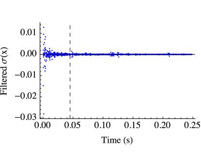
Figure 9: Plot of the filtered standard deviation of $\bar{q}$, the point of convergence is indicated by the vertical dashed line.

Once convergence is achieved, it is a simple matter to restart the process described above, finding a new value for $\bar{q}$. Figure 10 shows a sample run where the departure rate of data elements from a queue to the compute kernel. Within this figure the actual service rate is known (solid blue $y$-axis grid lines). The $x$-axis grid lines (dashed vertical lines) show where our method has converged to a stable solution and re-started. Changes in $\bar{q}$ are assumed to mean a change in the process distribution governing $tc$.

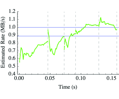
Figure 10: Example of $\bar{q}$ adapting to two service rates during execution of a micro-benchmark. The instrumentation captures the departure rate from a single queue to a compute kernel.

V Experimental Setup

V-A Infrastructure

The hardware used for all empirical evaluation is listed in Table III. All code is compiled with the “-O2” compiler flag using the GNU GCC compiler (version 4.8.3).

In order to assess our method over a wide range of conditions, a simple micro-benchmark consisting of two threads connected by a lock-free queue is used. Each thread consists of a while loop that consumes a fixed amount of time in order to simulate work with a known service rate. The amount of work, or service-rate, is generated using a random number generator sourced from the GNU Scientific Library [7]. The service rates of kernels within the micro-benchmark are limited to approximately $\sim 8$ MB/s due to the overhead of the random number generator and the size of the output item (8 bytes). Service time distributions are set as either exponential or deterministic. Parameterization of the distributions is selected using a pseudorandom number source. The exact parameterization range and distribution are noted where applicable within the results section.

TABLE III: Summary of hardware used for empirical evaluation

Platform	Processor	OS	Main Memory
1	2 $\times$ AMD Opteron 6136	Linux 2.6.32	62 GB
2	2 $\times$ Intel E5-2650	Linux 2.6.32	62 GB
3	2 $\times$ Intel Xeon X5472	Darwin 13.4.0	32 GB
4	2 $\times$ Six-Core AMD Opteron 2435	Linux 3.10.37	32 GB
5	Intel Xeon CPU E3-1225	Linux 3.13.9	8 GB

The streaming framework used is the RaftLib C++ template library [20]. The RaftLib framework previously included instrumentation for static service rate determination (i.e., by running each compute kernel individually with an infinite data source and infinitely large output queue). The functionality of online service rate determination as described by this work has also been incorporated into the platform.

V-B Applications

In addition to the micro-benchmarks described above, two full streaming applications are also explored. The first, matrix multiply, is a synchronous data flow application that is expected to have relatively stable service rates. The second is a string search application that has variable rates. Ground truth service rates for each kernel are determined by executing each kernel offline and measuring the rates individually using a large resident memory data source (constructed for each kernel) and ignoring the write pointers so that it simulates an infinite output buffer.

V-B1 Matrix Multiply

Matrix multiplication is central to many computing tasks. Implemented here is a simple dense matrix multiply ($C=AB$) where the multiplication of matrices $A$ and $B$ are broken into multiple dot-product operations. The dot-product operation is executed as a compute kernel with the matrix rows and columns streamed to it. This kernel can be duplicated $n$ times (see Figure 11). The result is then streamed to a reducer kernel (at right) which re-forms the output matrix $C$. This application differs from the micro-benchmarks in that it uses real data read from disk and performs multiple operations on it. As with the micro-benchmarks, it has the advantage of having a continuous output stream from both the matrix read and dot-product operations.

The data set used for the matrix multiply is a $10,000\times 10,000$ matrix of single precision floating point numbers produced by a uniform random number generator.

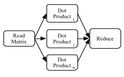
Figure 11: Matrix multiply application. The first kernel reads both matrices to be multiplied and streams the data to an arbitrary ($n$) number of dot product kernels. The final kernel reduces the input from the dot to a multiplied matrix.

V-B2 Rabin-Karp String Search

The Rabin-Karp [10] algorithm is classically used to search a text for a set of patterns. It utilizes a “rolling hash” function to efficiently recompute the hash of the text being searched as it is streamed in. The implementation divides the text to be searched with an overlap of $m-1$ (for a pattern length of $m$), so that a match at the end of one pattern will not result in a duplicate match on the next segment. The output of the rolling hash function is the byte position within the text of the match. The output of the rolling hash kernel is variable (dependent on the number of matches), for model selection testing purposes the input data will be specially constructed in order to produce a regular steady state output. The next kernel verifies the match from the rolling hash to ensure hash collisions don’t cause spurious matches. The verification matching kernel can be duplicated up to $j$ times. The final kernel simply reduces the output from the verification kernel(s), returning the byte position of each match (see Figure 12). The corpus consists of 2 GB of the string, “foobar.”

Figure 12: Rabin-Karp matching algorithm. The first compute kernel (at left) reads the file to be searched, hashes the patterns to search and distributes the data to $n$ “rolling-hash” kernel(s). Next are $j,j\leq n$ verification kernel(s) to guard against matches due to hash collision. The final kernel (at right) is a reducer which consolidates all the results.

VI Results

The methods that we have described are designed to enable online service rate determination. Just how well do these methods work in real systems while they are executing? In order to evaluate this quantitatively, several sets of micro-benchmarks and real applications are instrumented to determine the mean service rate of a given server. We start with two sets of micro-benchmarks, the first having a stationary distribution (with a fixed mean) and the second having a bi-modal distribution that shifts its mean halfway through its execution.

Each micro-benchmark is constructed with the configuration depicted in Figure 1 and executed with a fixed arrival process distribution. The service rate of Kernel B is varied for each execution of the micro-benchmark from ($0.8$ MB/s $\rightarrow\;\sim\!8$ MB/s). The results comprise $1800$ executions in total. The departure rate from the queue is instrumented to observe the service rate of Kernel B. The goal is to find the service rate of this kernel without a priori knowledge of the actual rate (which we are setting for this controlled experiment). Figure 13 is a histogram of the percent difference between the service rate estimated via our method and the “set” filtered rate.

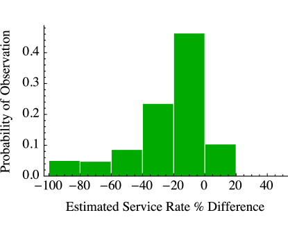
Figure 13: Histogram of the probability of estimating the service rate of Kernel B from Figure 1. Each execution is a data point, with the percent difference calculated as $(\frac{(\text{observed rate}-\text{set rate})}{\text{set rate}})\times 100$. Not plotted are four outliers to right of the plotted data which are greater than $1000\%$ difference, which is not unexpected given the probabilistic nature of our heuristic.

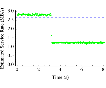
Figure 14: Depiction of the ideal (drawn from empirical data) of the instrumentation’s ability to estimate the service rate while the application is executing. Each dot represents the converged service rate estimate ($y$-axis). The top and bottom dashed lines represent the first and second phases as verified by manual measurement in isolation.

We see in this histogram that generally the correspondence between estimated service rate and ideal service rate is reasonably good. We expect divergence since these rates are determined while the application is executing, not the full execution time average rate. When it errs, the estimate is typically low, which is consistent with previous empirical data, in which actual realized execution times are typically longer than nominal [2]. The majority of the results are within 20% of nominal in any case. The computational environment of any given kernel can change from moment to moment. We simulate environment change by moving the mean of the distribution halfway through execution of Kernel B (with reference to the number of data elements sent). We are interested in whether our instrumentation can detect this change, potentially enabling many online optimizations. An ideal example with a wide switch in service rate is shown in Figure 14 where the first phase is at $\sim\!2.66$ MB/s and the second is much lower at $\sim\!1$ MB/s. Not all examples are so clear cut.

In order to classify the dual phase results into categories, a percent difference ($20\%$) from the manually determined rates for each phase is used. Approximately $14.7\%$ of the data had nominal service rate shifts that were known to be less than the $20\%$ criteria specified. Figure 15 shows the effectiveness of our technique in categorizing the distinct execution phases of the micro-benchmarks. The rightmost graph shows the categorizations for low $\rho$, and the leftmost graph shows the categorizations for high $\rho$. Here, we make two observations. First, the system correctly detects both phases more effectively in high utilization conditions, which are the conditions under which correct classification is likely to be more important. Second, the classification errors that are made are all conservative. That is, it is correctly detecting the final condition of the kernel, indicative of a conservative settling period for rate estimation.

It is well understood that a server with sufficient data on it’s input queue should be able to proceed with processing (assuming no other complicating factors). Therefore one trend that we expect to see is an improvement in the approximation for higher server utilizations. In addition, servers that are more highly utilized typically have a much more profound impact on the performance of the application as a whole (e.g., they are dramatically more likely to be throughput bottlenecks in the overall data flow).

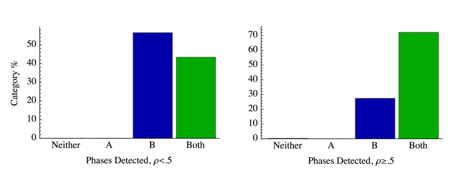
Figure 15: Data from a dual-phase micro-benchmark that generates two distinct service rate phases separated by server utilization, $\rho$, and then by correct classification at each phase (as “Neither,” “A,” “B,” or “Both”), which represent the heuristic finding none, only the first phase, only the second phase or both, respectively.

Overall, the heuristic did quite well. Looking at the single phase data, only four of the micro-benchmark results were extremely off. The dual phase data were also fairly good, the heuristic failed to find either phase in only $0.24\%$ of the instances. The real test of any instrumentation is how well it can handle situations beyond those that are carefully controlled. The only variable that is within the users’ control is that of data set selection. Notably these applications are not limited to the slower service rates of the micro-benchmark applications but are dependent on the mechanics of the application. The matrix multiply application is executed on platform 2 from Table III with the number of parallel dot-products set to five. Only the reduce kernel is instrumented (see Figure 11) as the dot-products would be rather easy given the high data rates inherent in transmitting an entire row by copy. The ground-truth service rate realized by each queue (the total service rate being a combination of rates from each input-queue) are determined by the method described in Section V-B1. Overall the results are not quite as clean as those of the microbenchmark, but that is expected given the chosen kernel has an extremely low $\rho$. A majority ($63\%$) are within the range of measurements observed during manual estimation removing each kernel from the system and manually measuring data rates at each input port).

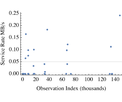
Figure 16: Plot of the trace for the instrumented partial service rate of the reduce kernel (the full rate being the sum of all rates for each in-bound queue). The manually determined rate for this experimental setup ranged from $0.05$ MB/s to $0.43$ MB/s. Overall, a majority of the results $\sim\!63\%$ are within this range.

Similar to the results for the matrix-multiply application, the results for the Rabin-Karp application are also relatively good (recall that these are rates taken at points over the course of execution). The application is executed on platform 2 from Table III with the number of matching kernels fixed at four and the number of verification kernels fixed to two. Figure 17 shows the online service rate by convergence point each data point represents a converged estimate of the service rate (potentially multiple convergences for a single application execution). Instrumented is a single queue arriving to the verify block from the hash kernel. Again, we’ve intentionally picked a case where the $\rho$ is very low, which is very difficult for the instrumentation to find a non-blocking read from the queue. In total, only $\sim\!35\%$ of estimates are within the range observed when manually measuring service rate, although most of the data points are fairly close. This highlights the limitations of our approach. If the non-blocking reads are not observed then the rate simply cannot be determined with too much accuracy.

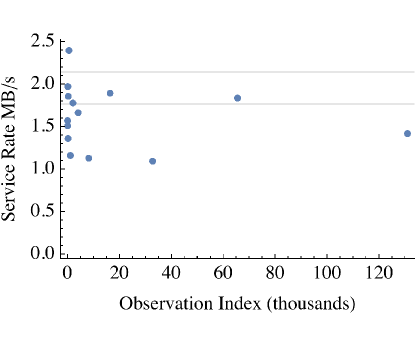
Figure 17: Plot of the converged estimates of service rate for a single queue within the Rabin-Karp string matching application. The utilization of this server is less than $0.1$ meaning that the queue is almost always empty which leads to less opportunity for recording non-blocking reads from the queue.

Low overhead instrumentation should be exactly that, low overhead. This means that there should be little, if any, impact on the execution of the application itself. Low impact also means that the system executing both the application and instrumentation should see as little increase in overhead as possible. Given that our system utilizes a separate monitor thread, this could be a concern. Using the single queue micro-benchmark, the impact was measured with instrumentation and without instrumentation. Using the GNU time command over dozens of executions, the average impact is only $1$ - $2\%$. Impact to the system overall was equally minimal, load average increased only a small amount (by $0.1$ on average).

VII Conclusions & Future Work

This paper proposes and demonstrates a heuristic that enables online service rate approximation of each compute kernel within a streaming system. In streaming systems that exhibit filtering, the heuristic presented here can also be used to detect non-blocking departure rates which can inform a run-time of routing decisions made by the kernel as well as the amount of filtering currently exhibited. Overall our methodology works quite well. When the heuristic fails, it usually fails knowingly (e.g., no convergence is reached or non-blocking reads were not observed). A few cases of non-convergence are included in the results (and noted). Currently the default in RaftLib is to fall back on the current best solution, but note the non-converged state. Future work might include the solutions mentioned in Section III (i.e., temporary throttling and duplication) which could improve the probability of convergence.

Alluded to earlier was the potential to estimate the likelihood of the distribution process modulating the data stream as matching a known distribution; which is quite useful if the known distribution enables the use of a closed form modeling solution. We’ve shown a heuristic that can estimate the central moment of the service process and it’s second moment (variance) in a streaming manner (for these calculations, only saving sums and discarding the actual values). Efficient methods also exist for streaming computation of higher moments [19]. Using the method of moments along with some simple classification, it should be clear that online distribution selection can be performed using the techniques described within this work as a basis, then extending them to include higher moment estimation. Future work, and extensions to the RaftLib instrumentation system, will include these pieces.

Parallelization decisions can easily benefit from the information that this method provides. Instead of relying on static (compile time) information, decisions can now be made with up-to-date data improving optimality of the execution. Related, but not shown here, is the ability of this process to instrument streams entering or exiting a TCP stack. It is assumed that there should be no difference in monitoring user-space queues feeding data into a TCP link. An open question is exactly how best to synchronize the ingress and egress transaction data.

In conclusion, we’ve demonstrated a probabilistic heuristic that under most conditions can estimate the service rate of compute kernels executing within a streaming system while that application is executing. It has been demonstrated to be effective using micro-benchmarks and two full stream processing applications on multi-core processors.

References

- [1] J. C. Beard and R. D. Chamberlain, “Analysis of a simple approach to modeling performance for streaming data applications,” in Proc. of IEEE Int’l Symp. on Modelling, Analysis and Simulation of Computer and Telecommunication Systems, Aug. 2013, pp. 345–349.
- [2] J. C. Beard and R. D. Chamberlain, “Use of a Levy distribution for modeling best case execution time variation,” in Computer Performance Engineering, ser. Lecture Notes in Computer Science, A. Horváth and K. Wolter, Eds., vol. 8721. Springer International Publishing, Sep. 2014, pp. 74–88.
- [3] J. C. Beard, P. Li, and R. D. Chamberlain, “Raftlib: A C++ template library for high performance stream parallel processing,” in Proc. of Programming Models and Applications on Multicores and Manycores. ACM, Feb. 2015, to appear.
- [4] J. Cadzow and H. Martens, Discrete-Time and Computer Control Systems. Englewood Cliffs: Prentice-Hall, 1970.
- [5] B. Cantrill, M. W. Shapiro, A. H. Leventhal et al., “Dynamic instrumentation of production systems.” in USENIX Annual Technical Conference, General Track, 2004, pp. 15–28.
- [6] T. F. Chan, G. H. Golub, and R. J. LeVeque, “Algorithms for computing the sample variance: Analysis and recommendations,” The American Statistician, vol. 37, no. 3, pp. 242–247, 1983.
- [7] M. Galassi, B. Gough, G. Jungman, J. Theiler, J. Davies, M. Booth, and F. Rossi, “The GNU scientific library reference manual, 2007,” http://www.gnu.org/software/gsl, accessed November 2014.
- [8] M. I. Gordon, W. Thies, and S. Amarasinghe, “Exploiting coarse-grained task, data, and pipeline parallelism in stream programs,” in Proc. of 12th Int’l Conf. on Architectural Support for Programming Languages and Operating Systems, 2006, pp. 151–162.
- [9] S. L. Graham, P. B. Kessler, and M. K. Mckusick, “Gprof: A call graph execution profiler,” ACM Sigplan Notices, vol. 17, no. 6, pp. 120–126, 1982.
- [10] R. M. Karp and M. O. Rabin, “Efficient randomized pattern-matching algorithms,” IBM Journal of Research and Development, vol. 31, no. 2, pp. 249–260, 1987.
- [11] M. Kendall and W. Buckland, A Dictionary of Statistical Terms. Edinburgh and London: Published for the International Statistical Institute by Oliver & Boyd, Ltd., 1957.
- [12] L. Kleinrock, Queueing Systems. Volume 1: Theory. Wiley-Interscience, 1975.
- [13] J. M. Lancaster, J. G. Wingbermuehle, and R. D. Chamberlain, “Asking for performance: Exploiting developer intuition to guide instrumentation with TimeTrial,” in Proc. 13th Int’l Conf. High Performance Computing and Communications, Sep. 2011.
- [14] S. S. Lavenberg, “A perspective on queueing models of computer performance,” Performance Evaluation, vol. 10, no. 1, pp. 53–76, 1989.
- [15] P. Li, K. Agrawal, J. Buhler, and R. D. Chamberlain, “Adding data parallelism to streaming pipelines for throughput optimization,” in Proc. of IEEE Int’l Conf. on High Performance Computing, 2013.
- [16] C.-K. Luk, R. Cohn, R. Muth, H. Patil, A. Klauser, G. Lowney, S. Wallace, V. J. Reddi, and K. Hazelwood, “Pin: building customized program analysis tools with dynamic instrumentation,” ACM Sigplan Notices, vol. 40, no. 6, pp. 190–200, 2005.
- [17] A. Mazouz, S.-A.-A. Touati, and D. Barthou, “Study of variations of native program execution times on multi-core architectures,” in Proc. of Int’l Conf. on Complex, Intelligent and Software Intensive Systems, 2010, pp. 919–924.
- [18] N. Nethercote and J. Seward, “Valgrind: a framework for heavyweight dynamic binary instrumentation,” ACM Sigplan Notices, vol. 42, no. 6, pp. 89–100, 2007.
- [19] P. Pébay, “Formulas for robust, one-pass parallel computation of covariances and arbitrary-order statistical moments,” Sandia Report SAND2008-6212, Sandia National Laboratories, 2008.
- [20] http://www.raftlib.io, accessed November 2014.
- [21] S. S. Shende and A. D. Malony, “The TAU parallel performance system,” International Journal of High Performance Computing Applications, vol. 20, no. 2, pp. 287–311, 2006.
- [22] B. Welford, “Note on a method for calculating corrected sums of squares and products,” Technometrics, vol. 4, no. 3, pp. 419–420, 1962.