A Markov model of a limit order book: thresholds, recurrence, and trading strategies

Abstract.

We analyze a tractable model of a limit order book on short time scales, where the dynamics are driven by stochastic fluctuations between supply and demand. We establish the existence of a limiting distribution for the highest bid, and for the lowest ask, where the limiting distributions are confined between two thresholds. We make extensive use of fluid limits in order to establish recurrence properties of the model. We use the model to analyze various high-frequency trading strategies, and comment on the Nash equilibria that emerge between high-frequency traders when a market in continuous time is replaced by frequent batch auctions.

1. Introduction.

A limit order book (LOB) is a trading mechanism for a single-commodity market. The mechanism is of significant interest to economists as a model of price formation. It is also used in many financial markets, and has generated extensive research, both empirical and theoretical: for a recent survey, see [11].

The detailed historic data from LOBs in financial markets has encouraged models able to replicate the observed statistical properties of these markets. Unfortunately, the added complexity usually makes the models less analytically tractable and, with relatively few exceptions, such models are explored by simulation or numerical methods. Our aim in this paper is to analyze a simple and tractable model of a LOB, first introduced by [22] and independently by [16] and by [19]. The basic form of the model explicitly excludes a number of significant features of real-world markets. Nevertheless we shall see that, from the model, several non-trivial and insightful results can be obtained on the structure of high-frequency trading strategies. Further, the model has a natural interpretation for a competitive and highly traded market on short time-scales, where the excluded features may be less significant. We believe the model may be helpful in discussions of market design, and as an illustration we use the model to comment on the Nash equilibria that emerge between high-frequency traders when a market in continuous time is replaced by frequent batch auctions.

To motivate the model consider a market with only two classes of participant. Firstly, long-term investors who place orders for reasons exogenous to the model, who view the market as effectively efficient for their purposes, and who do not shade their orders strategically. Temporary imbalances between supply and demand from such long-term investors will cause prices to fluctuate even in the absence of any new information becoming available concerning the fundamentals of the underlying asset. Our second class of participant, high-frequency traders, attempt to benefit from these price fluctuations by providing liquidity between the long-term investors. In practice we should expect a spectrum of behavior between these two extremes. The extreme case, with just long-term investors and high-frequency traders, is clearly a caricature, but we shall see that it does allow us to analyze various high-frequency trading strategies (for example market-making, sniping and mixtures of these) and the Nash equilibria between them.

We next describe the model of a LOB for an example involving long-term investors only, and outline our results for this example. A bid is an order to buy one unit, and an ask is an order to sell one unit. Each order has associated with it a price, a real number. Suppose that bids and asks arrive as independent Poisson processes of unit rate and that the prices associated with bids, respectively asks, are independent identically distributed random variables with density $f_{b}(x)$, respectively $f_{a}(x)$. An arriving bid is either added to the LOB, if it is lower than all asks present in the LOB, or it is matched to the lowest ask and both depart. Similarly an arriving ask is either added to the LOB, if it is higher than all bids present in the LOB, or it is matched to the highest bid and both depart. The LOB at time $t$ is thus the set of bids and asks (with their prices), and our assumptions imply the LOB is a Markov process.

For this model we show that there exists a threshold $\kappa_{b}$ with the following properties: for any $x<\kappa_{b}$ there is a finite time after which no arriving bids less than $x$ are ever matched; and for any $x>\kappa_{b}$ the event that there are no bids greater than $x$ in the LOB is recurrent. Similarly, with directions of inequality reversed, there exists a corresponding threshold $\kappa_{a}$ for asks. Further there is a density $\pi_{a}(x)$, respectively $\pi_{b}(x)$, supported on $(\kappa_{b},\kappa_{a})$ giving the limiting distribution of the lowest ask, respectively highest bid, in the LOB. The densities $\pi_{a},\pi_{b}$ solve the equations

(1a) $$f_{b}(x)\int_{x}^{\kappa_{a}}\pi_{a}(y)dy=\pi_{b}(x)\int_{-\infty}^{x}f_{a}(y)dy$$

(1b) $$f_{a}(x)\int_{\kappa_{b}}^{x}\pi_{b}(y)dy=\pi_{a}(x)\int_{x}^{\infty}f_{b}(y)dy.$$

As a specific example, if $f_{a}(x)=f_{b}(x)=1,x\in(0,1)$, then $\kappa_{a}=\kappa,\kappa_{b}=1-\kappa$, $\pi_{a}(x)=\pi_{b}(1-x)$, and

(2) $$\pi_{b}(x)=(1-\kappa)\left(\frac{1}{x}+\log\left(\frac{1-x}{x}\right)\right),\quad x\in(\kappa,1-\kappa)$$

where the value of $\kappa$ is given as follows. Let $w$ be the unique solution of $we^{w}=e^{-1}$: then $w\approx 0.278$ and $\kappa=w/(w+1)\approx 0.218$. Observe that any example with $f_{a}=f_{b}$ can be reduced to this example by a monotone transformation of the price axis.

The existence of thresholds with the claimed properties is a relatively straightforward result, using Kolmogorov’s 0–1 law. In order to make the claimed distributional result precise the major challenge is to establish positive recurrence of certain binned models: such models arise naturally where, for example, prices are recorded to only a finite number of decimal places. Given a sufficiently strong notion of recurrence the intuition behind equations (1) is straightforward: in equilibrium the right-hand side of equation (1a) is the probability flux that the highest bid in the LOB is at $x$ and that it is matched by an arriving ask with a price less than $x$, and the left-hand side is the probability flux that the lowest ask in the LOB is more than $x$ and that an arriving bid enters the LOB at price $x$; these must balance, and a similar argument for the lowest ask leads to equation (1b). To establish positive recurrence of the binned models we make extensive use of fluid limits (see [2]), an important technique in the study of queueing networks.

The orders we have described so far are called limit orders to distinguish them from market orders which request to be fulfilled immediately at the best available price. Market orders are straightforward to include in the model: in the specific example just described we simply associate a price $1$ or $0$ with a market bid or market ask respectively. As the proportion of market bids increases towards a critical threshold, $w\approx 0.278$ in the above example, the support of the limiting distributions $\pi_{a},\pi_{b}$ increases to approach the entire interval $(0,1)$: above the threshold the model predicts recurring periods of time when there will exist either no highest bid or no lowest ask in the LOB. This conclusion necessarily holds, with the same critical threshold $w$, for any example with $f_{a}=f_{b}$.

A LOB is a form of two-sided queue, the study of which dates at least to the early paper of [12], who modeled a taxi-stand with arrivals of both taxis and travellers as a symmetric random walk. Recent theoretical advances involve servers and customers with varying types and constraints on feasible matchings between servers and customers, with applications ranging from large-scale call centres to national waiting lists for organ transplants (cf. [1, 23, 27]). Our interest in models of LOBs is in part due to the simplicity of the matchings in this particular application: types, as real variables, are totally ordered and so when an arriving order can be matched the match is uniquely defined.

Next we comment on several important features of real-world markets that are missing from the above basic model of a LOB. We assume that orders (from investors) are never cancelled and that the arrival streams of orders, with their prices, are not dependent on the state of the LOB. These assumptions might be natural for orders from our long-term investors who view the market as effectively efficient for their purposes. These assumptions, and the related assumption of stationarity of the arrival streams, may also be natural for a high-volume market where there may be a substantial amount of trading activity even over time periods where no new information becomes available concerning the fundamentals of the underlying asset. Mathematically the model may then be viewed as assuming a separation between the time-scale of trading, represented in the model, and a longer time-scale on which fundamentals change.

The assumption that all orders are for a single unit is important mathematically for the derivation of equations (1); economically, it corresponds to an assumption of a competitive market where an investor does not need to think about the impact of her order size on the market. We note that a long-term investor placing a large order may attempt to be passive in her execution, so as not to move the price against her, by spreading the order in line with volume in the market; see [8]. The natural question then becomes over how long the order is spread, and the model can give insight here. We note, however, that our assumption of a separation between the time-scale of trading and the timescale on which fundamentals change, modeled by our assumption of stationarity of arrival streams, may no longer be tenable when the time taken by a large investor to complete an order increases. In markets with a relatively small set of participants with large orders other approaches may be necessary; see [7] for a discussion of trading protocols that complement limit order books for large strategic investors.

Markets may contain traders other than long-term investors, and there is currently considerable interest in the effect of high-frequency trading on LOBs. Importantly, many high-frequency trading strategies are straightforward to represent within the model, since traders who can react immediately to an order entering the LOB may leave the Markov structure intact. Consider first the following sniping strategy for a single high-frequency trader: she immediately buys every bid that joins the LOB at price above $q$ and every ask that joins the LOB at price below $p$, where $p$ and $q$ are chosen to balance the rates of these purchases. This model fits straightforwardly within our framework, and we show how to calculate the optimal values, for the high-frequency trader, of the constants $p$ and $q$. A single trader might instead behave as a market maker and place an infinite number of bid, respectively ask, orders at $p$, respectively $q$, where $\kappa_{b}<p<q<\kappa_{a}$. We are again able to analyze this case. The optimal profit rate under the sniping strategy may beat that under the market making strategy: it does so for the specific example above where $f_{a}(x)=f_{b}(x)=1,x\in(0,1)$, describes the order flow from long-term investors. But a third strategy, which combines market making and sniping, will generally beat both the individual strategies.

The model also allows us to readily explore the equilibria that emerge when there are multiple high-frequency traders competing using market making or sniping strategies. There has been considerable discussion recently of the effects of competition between multiple high-frequency traders, and of proposals aimed to slow down markets. A key issue is that high-frequency traders may wastefully compete on the speed with which they can snipe an order, and as a regulatory response Budish et al. [3, 4] propose replacing a market continuous in time with frequent batch auctions, held perhaps several times a second. We consider Nash equilibria in continuous and batch markets when there are multiple high-frequency traders competing using mixtures of market making and sniping. Competition between market making traders reduces the bid-ask spread and the traders’ profit rate, and does so whether the market is continuous or batch. Competition between sniping traders in a batch market results in a Nash equilibrium with traders sniping bids above, respectively asks below, a central price; the traders’ profit rate is slightly less in a batch market than a continuous market.

Competition between sniping strategies produces a large number of cancelled orders since if a strategy’s attempt to snipe an arriving order is not successful then the strategy immediately cancels its own order. A notable feature of data from real LOBs, that a substantial proportion of orders are immediately cancelled [11], thus emerges as a deduction from, rather than an assumption of, the model.

A discrete version of the model was first proposed by [22] in his pioneering work on regulation of securities markets, and the model was independently introduced by [16] and by [19]. Taking stationarity as an assumption, [16] provided an extensive analysis of the model; our equations (1) can be deduced from [16, Proposition 1], assuming steady-state behavior, by setting time derivatives to zero. Our contribution is to establish the existence of the thresholds $\kappa_{a},\kappa_{b}$ and to prove a sufficiently strong notion of recurrence to justify the intuition behind equations (1).

Previous research similar in mathematical framework to that reported here is by Cont and coauthors [6, 5], by Simatos and coauthors [21, 14] building on Lakner et al. [15], and by Toke [25]: as we do, these authors describe LOBs as Markovian systems of interacting queues and are able to obtain analytical expressions for various quantities of interest. In the models of [6, 5, 15, 21, 14] the arrival rates of orders at any given price depends on how far the price is above or below the current best ask or bid price; the models of [15, 21, 14, 25] are one-sided in that all bids are limit orders and all asks are market orders. Gao et al. [10] study the temporal evolution of the the shape of a LOB in the model of [6], under a scaling limit. Maglaras et al. [17] study a fragmented one-sided market in which traders may route their orders to one of several exchanges. The work of Lachappelle et al. [13], building on Roşu [20], uses a different mathematical framework, that of a mean field game, but shares with our approach some important features. In particular, these authors distinguish between institutional investors whose decisions are independent of the immediate state of the LOB and high-frequency traders who trade as a consequence of the immediate state of the LOB. The models of both [5] and [13] keep detailed information on queue sizes only at the best bid and best ask prices; [6] shares with our approach a Markov description of the entire LOB.

In much of the market microstructure literature features of LOBs, such as large bid-ask spreads, are explained as a consequence of participants protecting themselves from others with superior information. While this is clearly an important aspect of real-world markets we note that such features may also arise from simpler models. The driving force for the dynamics of the LOB in our approach, as in [13, 20], is not asymmetric information but stochastic fluctuations between supply and demand.

The organisation of the paper is as follows. In Section 2 we describe precisely the model and our main results. Section 3 develops the scaffolding necessary for the proofs, which are given in Section 4. In Section 5 we describe some applications of our results: this section contains our discussion of market orders, and of high-frequency trading strategies and Nash equilibria.

2. Model and results.

The state of the LOB at time $t$ is a pair $(B_{t},A_{t})$ of (possibly infinite) counting measures on ${\mathbb{R}}$; $B_{t}$ represents the prices of queued (not yet executed) bid orders, and $A_{t}$ represents the prices of queued asks. New orders arrive as a labeled point process; the label records the type of order (bid or ask) and the price. Without loss of generality, we assume that the price axis has been continuously reparametrized so that all prices fall in the interval $(0,1)$ (or, occasionally, $[0,1]$).

Orders depart from the queue when an arriving order “matches” one of the orders already in the book. We shall need several notions of what it means for two prices to match, and to capture this we introduce a price equivalence function, that is a nondecreasing, not necessarily continuous, function ${\mathcal{P}}:[0,1]\to[0,1]$. A bid-ask pair is compatible if ${\mathcal{P}}(\text{bid})\geq{\mathcal{P}}(\text{ask})$.We shall primarily consider two types of price equivalence function: ${\mathcal{P}}(x)=x$, and the function that partitions all prices into $n$ pricing bins. We will refer to the latter case, where the image of ${\mathcal{P}}$ is a finite set, as the binned model. Note that the same price equivalence function is applied to the prices of all the orders, and compatibility of bid-ask pairs is unchanged under any strictly increasing transformation of the equivalence function.

We are now ready to formally define the evolution limit order book ${\mathcal{L}}_{t}$.

Initial state: Initially, there should be no compatible bid–ask pairs in the book. Equivalently, the initial state $(B_{0},A_{0})$ satisfies

$$B_{0}[x,1)\cdot A_{0}(0,y]=0\quad\text{ if }\quad{\mathcal{P}}(y)\leq{\mathcal{P}}(x).$$

Most of the time we assume that the total number of orders in the book is finite; we relax this assumption in Section 5, where we allow an infinite number of orders to be placed at a single price, and otherwise the book is finite.

Order arrival process: New orders arrive as a Poisson process with iid labels designating the type and price of the order. Unless specified otherwise, we assume that ${\mathbb{P}}(\text{bid})={\mathbb{P}}(\text{ask})=1/2$. We assume the labels of orders are independent and identically distributed, and in particular independent of the state of the book, but the distributions of prices may depend on type. We let $F_{a}$ be the CDF of prices of arriving asks, and $F_{b}$ be the CDF of prices of arriving bids. We will often assume that the distributions of the prices of arriving orders have densities $f_{a}$ and $f_{b}$ respectively; this entails no loss of generality, because the LOB evolution is defined by the combination of the arriving price distributions and a price equivalence function, and thus we can always assume that the arriving orders have densities and only become discontinuous after being put through the price equivalence function.

Change at order arrival: We do not allow cancellations in the model (until Section 5), so all changes to the state occur at the time of an order arrival. Suppose at time $t$ a bid at price $p$ arrives. If there is a matching ask in the book, i.e. if $A_{t-}(0,y]>0$ for some $y$ such that ${\mathcal{P}}(y)\leq{\mathcal{P}}(x)$, then nothing happens to the bids in the book ($B_{t}=B_{t-}$), and the lowest ask departs: $A_{t}=A_{t-}-\delta_{q}$, where $q=\min\{x:A_{t-}\{x\}>0\}$ . If there are no matching asks in the book, the bid joins the book: $B_{t}=B_{t-}+\delta_{p}$ and $A_{t}=A_{t-}$. The situation is symmetric if the arriving order is an ask at price $q$: if there is a matching bid, the two orders depart (so $A_{t}=A_{t-}$ and $B_{t}=B_{t-}-\delta_{p}$ where $p=\max\{x:B_{t-}\{x\}>0\}$), and if there are no matching bids, then the ask joins the book ($B_{t}=B_{t-}$ and $A_{t}=A_{t-}+\delta_{q}$).

We will be keeping track of the highest (price of a) bid $\beta_{t}$ and lowest (price of an) ask $\alpha_{t}$ in the book at time $t$. If an order departs the book at time $t$, it must be at price $\beta_{t-}$ (if a bid) or $\alpha_{t-}$ (if an ask). We allow $B_{0}\{x\}=\infty$ or $A_{0}\{y\}=\infty$; if this is the case, then no bids left of $x$, and no asks right of $y$, will ever depart the limit order book, since they will never be the highest bid (respectively lowest ask).

Below, we will refer to continuous and discretized models of LOBs. A continuous LOB is one where the order price densities $f_{a}$ and $f_{b}$ (exist and) are bounded above and below, and the price equivalence function is ${\mathcal{P}}(x)=x$. Discretized models will use some binned price equivalence function, and will sometimes (but not always) assume that all bins receive a positive proportion of the orders of each type.

For a discretized, binned LOB, we will use notation $\llbracket x\rrbracket$ to denote the index of the bin containing $x$; $\llbracket x\rrbracket$ is a positive integer ranging from 1 to $N$ for some $N>0$.

We now present the main results concerning the model. The first result, Theorem 2.1, establishes a transition at threshold values $\kappa_{b}$ and $\kappa_{a}$. Eventually bids arriving below $\kappa_{b}$, and asks arriving above $\kappa_{a}$, will never be executed; whereas all bids arriving above $\kappa_{b}$, and all asks arriving below $\kappa_{a}$, will be executed. The second result, Theorem 2.2, presents the distribution of the rightmost bid and leftmost ask.

Theorem 2.1 (Thresholds).

There exist prices $\kappa_{b}$ and $\kappa_{a}$ with the following properties:

1. For any $\epsilon>0$ there exists, almost surely, a (random) time $T_{0}<\infty$ such that $\beta_{t}>\kappa_{b}-\epsilon$ and $\alpha_{t}<\kappa_{a}+\epsilon$ for all $t\geq T_{0}$.

2. For any $\epsilon>0$, infinitely often there will be no orders with prices in $(\kappa_{b}+\epsilon,\kappa_{a}-\epsilon)$.

3. Let $x>\kappa_{b}+\epsilon$ and $y<\kappa_{a}-\epsilon$ for some $\epsilon>0$. Consider the LOB started with infinitely many bids at $x$, infinitely many asks at $y$, and finitely many orders in between. The evolution of the orders at prices in the interval $(x,y)$ is a positive (Harris) recurrent Markov process, with finite expected time until there are no orders in the interval.

The fact that there will infinitely often be no bids above $x$, and no asks below $y$, is a consequence of Kolmogorov’s 0–1 law; the challenge is to show that there will simultaneously be neither bids nor asks in the interval $(x,y)$. In fact, we shall need to prove this part of Theorem 2.1 and Theorem 2.2 below in tandem.

Theorem 2.2 (Distribution of the highest bid).

Consider a continuous LOB; that is, ${\mathcal{P}}(x)=x$, and the densities $f_{b}$ and $f_{a}$ are bounded above and below. Then

1. The limiting distributions of the highest bid and lowest ask have densities, denoted $\pi_{b}$ and $\pi_{a}$; let $\varpi_{b}=\pi_{b}/f_{b}$ and $\varpi_{a}=\pi_{a}/f_{a}$.

2. The thresholds satisfy $0<\kappa_{b}<\kappa_{a}<1$, and also $F_{b}(\kappa_{b})=1-F_{a}(\kappa_{a})$.

3. The distribution of the highest bid is such that $\varpi_{b}$ is the unique solution to the ordinary differential equation

   $$\left(-\frac{f_{a}(x)}{1-F_{b}(x)}(F_{a}(x)\varpi_{b}(x))^{\prime}\right)^{\prime}=\varpi_{b}(x)f_{b}(x)$$

   with initial conditions

   $$(F_{a}(x)\varpi_{b}(x))|_{x=\kappa_{b}}=1,\qquad(F_{a}(x)\varpi_{b}(x))^{\prime}|_{x=\kappa_{b}}=0$$

   and the additional constraint $\varpi_{b}(x)\to 0$ as $x\uparrow\kappa_{a}$. The distribution of the lowest ask is determined by a similar ODE.

Corollary 2.3 (Uniform arrivals).

Suppose that ${\mathcal{P}}(x)=x$ and the arrival price distribution is uniform on $(0,1)$ for both bids and asks. Then $\kappa_{b}=\kappa\approx 0.218$ is given by $\kappa=w/(w+1)$ where $we^{w}=e^{-1}$. The limiting density of the highest bid is supported on $(\kappa,1-\kappa)$, and is given by

$$\varpi_{b}(x)={\mathbf{1}}_{(\kappa,1-\kappa)}(1-\kappa)\left(\frac{1}{x}+\log\left(\frac{1-x}{x}\right)\right)$$

and the limiting density of the lowest ask is $\varpi_{a}(x)=\varpi_{b}(1-x)$.

Remark 1 (Absolute continuity).

We can replace conditions on the densities $f_{a}$ and $f_{b}$ by the requirement that $dF_{a}/dF_{b}$ be bounded above and below; however, it is more natural to state the result of Theorem 2.2 in terms of densities. The boundedness requirement avoids the trivial counterexamples $f_{b}=2{\mathbf{1}}_{[0,1/2)}$, $f_{a}=2{\mathbf{1}}_{(1/2,1]}$ (nonoverlapping supports, no orders leave) or $f_{a}=2{\mathbf{1}}_{[0,1/2)}$, $f_{b}=2{\mathbf{1}}_{(1/2,1]}$ (nonoverlapping supports, no threshold).

Through a reparametrization of the price axis, Corollary 2.3 covers all cases where arriving bid and ask prices have identical densities. We describe some other analytically tractable applications of Theorem 2.2 in Section 5. We shall also, in Section 5, extend the analysis to deal with some examples where the supports of the bid and ask price distributions do not coincide.

Remark 2.

The form of the limiting density appearing in Corollary 2.3 can be deduced from equations (63)–(64) of [16, Section 3] after applying a coordinate transformation to convert between $[0,\infty)$ and $[0,1)$.

In Figure 1, we show the exact limiting distribution of the highest bid for the binned LOB with uniform arrivals over 50 bins, along with the limiting distribution for the continuous LOB. Note the “shoulder” bin: in the binned LOB, the threshold happens to fall into the middle of a bin, so the long-term probability of having the rightmost bid in the bin is positive but below the continuous limit.

Figure 1. Limiting density of the highest bid for the binned LOB with 50 bins, and limiting density for a continuous LOB (dotted line). Note the “shoulder” bin in the binned model: the threshold in the continuous LOB lies in the interior of this bin.

While we have been able to compute analytically the distribution of the location of the rightmost bid, there are many related quantities for which we do not have exact expressions in steady-state (although the positive recurrence established in Theorem 2.1 implies that they are well-defined and can be estimated consistently from simulation). Notably, except in the special case to be considered in Section 5.1.3, we have not been able to derive analytic expressions for the equilibrium height of the book (i.e. expected number of bids or asks at a given price in the binned model), or for the joint distribution of the highest bid and lowest ask. For an illustration of the simulated joint density of the highest bid and lowest ask, see [26].

2.1. Brief summary of notation

We summarize here our notation, as well as some of the main assumptions used in the text.

${\mathcal{L}}$: limit order book.
${\mathcal{P}}$: price equivalence function, a monotone increasing function. Most of the time we use either ${\mathcal{P}}(x)=x$ or the function that places all prices into one of several bins.
$A_{t}$, $B_{t}$: the counting measure of asks, respectively bids, at time $t$.
$F_{a}$, $F_{b}$: CDFs of the prices of arriving ask and bid orders. Until Section 5.1.1, newly arriving orders are assumed to have equal probability of being a bid or an ask. In a binned model, we may write $F_{a,b}(n)$ (with $n$ an integer) to refer to the fraction of orders arriving into bins with index $\leq n$, i.e. the CDF evaluated at the rightmost endpoint of the interval.
$f_{a}$, $f_{b}$: the corresponding densities, which are assumed to exist. For most results, $f_{a}$ and $f_{b}$ are assumed to be bounded above and below.
$\alpha_{t}$, $\beta_{t}$: the price of the lowest ask, respectively highest bid, at time $t$. Note that this is the actual price, not the bin containing it.
$\llbracket x\rrbracket$: in a binned LOB, the index of the bin containing price $x$.
$\kappa_{a}$, $\kappa_{b}$: limiting prices above (respectively below) which only finitely many asks (bids) are ever executed. It is not obvious a priori that $\kappa_{a}<1$ or $\kappa_{b}>0$; we prove this fact in Step 3 of the proof of Proposition 4.2.
For functions of two or more arguments, we may interchange arguments and subscripts: thus, $f_{k,n}(t)\equiv f_{n}(k,t)\equiv f(k,n,t)$. We will use notation $f_{n}(k,\cdot)$ when we wish to consider $f$ as a function of the third argument alone.

3. Preliminary results: monotonicity.

Before proving the main results, we erect some scaffolding. Part of its purpose is to allow us to transition between continuous LOBs (for which we expect to get differential equations in the answer) and binned models (which can be modeled as countable-state Markov chains). It will also allow us to compare LOBs with different arrival price distributions.

Lemma 3.1 asserts that the state of the limit order book is Lipschitz in the initial state with Lipschitz constant 1: in particular, small perturbations in the arrival and matching patterns will lead to small perturbations in the state of the book. Lemma 3.2 asserts that actions that decrease cumulative bid and ask queues by either shifting orders or removing them in bid–ask pairs will only decrease future queue sizes.

Lemma 3.1 (Adding one order).

Consider a limit order book ${\mathcal{L}}$, and let $\tilde{\mathcal{L}}$ differ from ${\mathcal{L}}$ by the addition of one bid at time 0; let their arrival processes and price equivalence functions be the same. Then at all times $\tilde{\mathcal{L}}$ differs from ${\mathcal{L}}$ either by the addition of one bid or by the removal of one ask.

Proof.

Proof. The roles of “bid” and “ask” are symmetric here. The claim clearly holds until the additional bid is the highest bid that departs from the system; once it does, ${\mathcal{L}}$ differs from $\tilde{\mathcal{L}}$ by the addition of a single ask, and the result follows by induction.∎

Define cumulative queue sizes $Q_{b}(p,t)=B_{t}(0,p]$, $Q_{a}(p,t)=A_{t}[p,1)$. (Note that we count bids from the left and asks from the right.) When we want to highlight the dependence on only one of the variables, we will drop the other variable into a subscript.

Lemma 3.2 (Decreasing queues).

Consider a limit order book ${\mathcal{L}}$, and let $\tilde{\mathcal{L}}$ differ from ${\mathcal{L}}$ by modifying the initial state in such a way that $\tilde{Q}_{b}(\cdot,0)\leq Q_{b}(\cdot,0)$, $\tilde{Q}_{a}(\cdot,0)\leq Q_{a}(\cdot,0)$ (as functions of price), and also $\tilde{Q}_{b}(1,0)-\tilde{Q}_{a}(0,0)=Q_{b}(1,0)-Q_{a}(0,0)$. In words, to get from ${\mathcal{L}}$ to $\tilde{\mathcal{L}}$, at time 0 we remove some bid–ask pairs, and/or shift some bids to the right, and/or shift some asks to the left. Then at all future times $t\geq 0$, $\tilde{Q}_{b}(\cdot,t)\leq Q_{b}(\cdot,t)$ and $\tilde{Q}_{a}(\cdot,t)\leq Q_{a}(\cdot,t)$ as functions of price.

Proof.

Proof. We show $\tilde{Q}_{b}\leq Q_{b}$, the argument for asks being identical. The argument proceeds by induction on time, i.e. the number of arrived orders. Throughout the proof, we use notation $f_{t-}=\lim_{s\searrow t}f(s)$ for the left limit of a càdlàg function $f$.

Consider first the arrival of a bid at time $t$ and price $p$. For it to upset the inequality, it must stay in $\tilde{\mathcal{L}}$ but depart immediately in ${\mathcal{L}}$; additionally, we need $Q_{b}(q,t-)=\tilde{Q}_{b}(q,t-)$ for some $q\geq p$. Note that if the bid departs immediately in ${\mathcal{L}}$, the leftmost ask at $\alpha_{t-}$ must be compatible with $p$, and in particular there are no bids right of $p$: $Q_{b}(p,t-)=Q_{b}(1,t-)$. This, together with $Q_{b}(q,t-)=\tilde{Q}_{b}(q,t-)$ and $\tilde{Q}_{b}(\cdot,t-)\leq Q_{b}(\cdot,t-)$, implies that $Q_{b}(1,t-)=\tilde{Q}_{b}(1,t-)$. Since bid–ask departures occur in pairs, this in turn implies $Q_{a}(0,t-)=\tilde{Q}_{a}(0,t-)$. But it is easy to see that if $\tilde{Q}_{a}(\cdot,t-)\leq Q_{a}(\cdot,t-)$ and they are equal at $0$, then $\tilde{\alpha}_{t-}$ (the leftmost jump of $\tilde{Q}_{a}(\cdot,t-)$) and $\alpha_{t-}$ (the leftmost jump of $Q_{a}(\cdot,t-)$) satisfy $\tilde{\alpha}_{t-}\leq\alpha_{t-}$, and hence the arriving bid actually departs immediately in $\tilde{\mathcal{L}}$ as well.

Next consider the arrival of an ask at time $t$ and price $p$. For it to upset the inequality, it must cause the departure of the highest bid in ${\mathcal{L}}$, but not in $\tilde{\mathcal{L}}$, and we must have $Q_{b}(q,t-)=\tilde{Q}_{b}(q,t-)$ for some $q\geq\beta_{t-}$ with ${\mathcal{P}}(\beta_{t-})\geq{\mathcal{P}}(p)$. Now, in $\tilde{\mathcal{L}}$ there are no bids at prices $\geq{\mathcal{P}}(p)$, hence $\tilde{Q}_{b}(1,t-)=\lim_{\epsilon\to 0}\tilde{Q}_{b}(p-\epsilon,t-)$. However, this contradicts the inequality $\tilde{Q}_{b}(\cdot,t-)\leq Q_{b}(\cdot,t-)$, since $\lim_{\epsilon\to 0}Q_{b}(p-\epsilon,t-)\leq\lim_{\epsilon\to 0}Q_{b}(\beta_{t-}-\epsilon,t-)\leq Q_{b}(1,t-)-1$. (Note that inequalities may not be equalities if there are multiple bids at the same price.)∎

We can use this lemma to compare two limit order books ${\mathcal{L}}$ and $\tilde{\mathcal{L}}$ with identical initial states and order arrival processes, but different price equivalence functions. Suppose the price equivalence function $\tilde{\mathcal{P}}$ merges some of the values that were distinguished by ${\mathcal{P}}$. Then any bid–ask pair that is compatible in ${\mathcal{L}}$ is also compatible in $\tilde{\mathcal{L}}$; and possibly additional bid–ask pairs are compatible in $\tilde{\mathcal{L}}$ as well. This lets us apply Lemma 3.2 to conclude that fewer orders will be present in $\tilde{\mathcal{L}}$.

We can give an upper bound on the queue sizes in ${\mathcal{L}}$ by using a binned LOB with one more bin and a shifted arrival process. If ${\mathcal{L}}$ has a bid arrival at price $x$ in bin $k=\llbracket x\rrbracket$, we let $\widehat{\mathcal{L}}$ have a bid arrival at some price in bin $k-1$. The ask arrivals are identical in ${\mathcal{L}}$ and $\widehat{\mathcal{L}}$. (If bins of ${\mathcal{L}}$ are numbered 1 through $N$, then bins of $\widehat{\mathcal{L}}$ are numbered $0$ through $N$; bids arrive into bins 0 through $N-1$ in $\widehat{\mathcal{L}}$, while asks arrive into bins 1 through $N$.) Under this arrangement, any bid–ask pair that is compatible in $\widehat{\mathcal{L}}$ was compatible in ${\mathcal{L}}$ as well, so $\tilde{\mathcal{L}}$ offers an upper bound on the queue sizes of ${\mathcal{L}}$. Consequently we can bound a continuous LOB ${\mathcal{L}}$ both from above and from below by two binned LOBs with slightly different arrival price distributions. (Assuming the continuous LOB has arrival distributions supported on $[0,1]$, the binned LOB providing the upper bound will have bid arrival distribution supported on $[-\epsilon,1-\epsilon]$ and ask arrival distribution supported on $[0,1]$.)

Finally, when bin sizes are small, the difference in the arrival price distributions will be small, and we’ll use Lemma 3.1 to bound the rate at which the states of $\tilde{\mathcal{L}}$ and $\widehat{\mathcal{L}}$ diverge. This will let us show that the behavior of the continuous LOB converges in a suitable sense.

4. Proof of main results.

We begin by stating a weaker form of Theorem 2.1.

Proposition 4.1 (Weak thresholds).

There exist prices $\kappa_{b}$ and $\kappa_{a}$ with the following properties:

1. For any $\epsilon>0$ there exists, almost surely, a (random) time $T_{0}<\infty$ such that $\beta_{t}>\kappa_{b}$ and $\alpha_{t}<\kappa_{a}$ for all $t\geq T_{0}$.

2. For any $\epsilon>0$, infinitely often there will be no bids with price exceeding $\kappa_{b}+\epsilon$. Similarly, infinitely often there will be no asks with price below $\kappa_{a}-\epsilon$.

3. The threshold values $\kappa_{b}$ and $\kappa_{a}$ satisfy $F_{b}(\kappa_{b})=1-F_{a}(\kappa_{a})$.

In addition, suppose that the bid and ask price densities (exist and) are bounded above by $M$. Then the following holds:

1. For any $\epsilon>0$, with probability 1, there exists a sequence of times $T_{n}\to\infty$ such that at time $T_{n}$ there are no bids with prices above ${\mathcal{P}}(\kappa_{b})+\epsilon$, and the number of asks with prices below ${\mathcal{P}}(\kappa_{a})-\epsilon$ is bounded above by $2(M+1)\epsilon T_{n}$.

Remark 3.

Although the compatibility of bid–ask pairs is driven by the price equivalence function ${\mathcal{P}}(x)$, the statements about $\kappa$ are in terms of $x$ itself. This is because whenever there are compatible bid–ask pairs, the bid with the highest value of $x$ and the ask with the lowest value of $x$ always depart the book. In particular, in a binned model, $\kappa_{b}$ and $\kappa_{a}$ will usually fall in the middle of some bin; in this “shoulder” bin, a nontrivial fraction of the arriving orders remain in the book forever. In Figure 1, $\kappa_{b}$ is approximately half-way through the “shoulder” bin. (It is also possible for $\kappa_{b}$ to form the edge of a bin.)

Remark 4.

Note that we make no assertions here about the behavior of $n^{-1}T_{n}$ as $n\to\infty$: for the purposes of this proposition, this sequence may well tend to zero. The proof of Theorem 2.1 will show that for any $\epsilon>0$ the sequence $n^{-1}T_{n}=n^{-1}T_{n}(\epsilon)$ is in fact eventually bounded away from zero, with the bound depending on $\epsilon$.

Proof.

Proof. The first two claims follow from Kolmogorov’s 0–1 law. Consider the events

$${\mathcal{E}}_{b}(x)=\{\text{finitely many bids will depart from prices $\leq x$}\}$$

$${\mathcal{E}}_{a}(x)=\{\text{finitely many asks will depart from prices $\geq x$}\}.$$

Lemma 3.1 shows that these events are in the tail $\sigma$-algebra of the arrival process. Since the arrival process consists of a sequence of independent and identically distributed events, Kolmogorov’s 0–1 law ensures that for each $x$, ${\mathcal{E}}_{b}(x)$ has probability 0 or 1 (and similarly for ${\mathcal{E}}_{a}(x)$). Now let

(3a) $$\kappa_{b}=\sup\{x:{\mathbb{P}}({\mathcal{E}}_{b}(x))=1\},\qquad\kappa_{a}=\inf\{x:{\mathbb{P}}({\mathcal{E}}_{a}(x))=1\}.$$

(If the set whose extremum is to be taken is empty, we let $$\kappa_{b}=0 \kappa_{a}=1 {\mathcal{E}}_{b}(x)\subseteq{\mathcal{E}}_{b}(y) x\geq y x x$$ or .) The first two asserted properties now follow upon noticing that for , and that whenever there is a bid departure at price , there must be no bids at prices higher than . (The situation is similar for asks.)

We next show that $F_{b}(\kappa_{b})+F_{a}(\kappa_{a})=1$. From the strong law of large numbers for the arrival process and the 0–1 law above, we know that $F_{b}(\kappa_{b})$ is the smallest limiting proportion of arriving bids that stay in the system:

(3b) $$F_{b}(\kappa_{b})=\lim\inf_{t\to\infty}\frac{1}{t}\#(\text{bids in the LOB at time $t$}).$$

A similar equality clearly holds for asks with $1-F_{a}(\kappa_{a})$. Since bids and asks always depart in pairs, a further appeal to the strong law of large numbers for the arrival process shows that we must have $F_{b}(\kappa_{b})=1-F_{a}(\kappa_{a})$.

The existence of times $T_{n}$ as in part (4) of the theorem follows by a similar argument from the functional law of large numbers for the arrival processes. With probability 1, picking a large enough time $T_{n}$ when there are no bids at prices above ${\mathcal{P}}(\kappa_{b})+\epsilon$ ensures that there are at most $(F_{b}(\kappa_{a})+(M+1)\epsilon)T_{n}$ asks in the system. Since asks to the right of $\kappa_{a}$ arrive at rate $(1-F_{a}(\kappa_{a}))=F_{b}(\kappa_{b})$ and eventually never leave, for large enough $T_{n}$ there will be at most $2(M+1)\epsilon T_{n}$ asks at prices below $\kappa_{a}-\epsilon$.∎

This result is weaker than the positive recurrence we wish to prove eventually: in particular, it does not show that the total number of both types of orders between $\kappa_{b}$ and $\kappa_{a}$ is ever zero. To obtain statements about positive recurrence, we shall need to use fluid limit techniques, and our overall approach will be similar to that in [2, Chapter 4]. The final proof of stability will use multiplicative Foster’s criterion (state-dependent drift), see [18, Theorem 13.0.1]. In order to get there, we need to show that whenever there are many bids or asks in $(\kappa_{b},\kappa_{a})$, their number tends to decrease at some positive, bounded below, rate over long periods of time. This is a standard line of argument in queueing theory; but the challenge of the model is that the evolution of the queues depends on which queues are positive, rather than which queues are large. In general Markov chains of this form are very difficult to analyze ([9] show that in general the stability of such chains is undecidable), but the special structure of our chain makes it amenable to analysis. The outline of the proof is as follows.

1. We work with binned LOBs. We begin by showing that, after appropriate rescaling, both the queue sizes and the local time of the highest bid (lowest ask) in each bin converge to a set of Lipschitz trajectories, which we call fluid limits. We then proceed to develop properties of the fluid limits.

2. We next show that all fluid limits tend to zero for bins (strictly) between $\llbracket\kappa_{b}\rrbracket+1$ and $\llbracket\kappa_{a}\rrbracket-1$. We exploit the equations and inequalities satisfied by fluid limits to show the following:

   1. There is an interval $[x_{0},y_{0}]$ on which, whenever the fluid limit of the number of orders is positive, it decreases (at a rate bounded below). Therefore, after some time $T_{0}$ (which depends on the initial state), the fluid limit will be zero on $[x_{0},y_{0}]$. The values $x_{0}$ and $y_{0}$ may not be bin boundaries.

   2. Following $T_{0}$, we will be able to bound from below the rate of increase of the local time of the rightmost bid on $[x_{1},x_{0})$ for some $x_{1}<x_{0}$, and of the leftmost ask on $(y_{0},y_{1}]$ for some $y_{1}>y_{0}$. Since whenever the highest bid is in $[x_{1},x_{0})$ it has a positive chance of departing (and similarly for asks in $(y_{0},y_{1}]$), we conclude that whenever the number of orders in $[x_{1},y_{1}]$ is large, it will decrease (at a rate bounded below). We repeat the argument until $[x_{n},y_{n}]\approx[\kappa_{b},\kappa_{a}]$. The $x_{i}$ and $y_{i}$ may not be bin boundaries in this step.

3. We show that if on some interval, all fluid limits converge to 0 in finite time, then the binned LOB is recurrent on that interval. (This step is standard for fluid limit arguments.) Since the number of bids in a continuous limit order book can be bounded from above by binned ones, this will also show recurrence of the continuous LOB.

4.1. ODE of the limiting distribution.

Our first result shows that the ODE which should describe the unique limit, as $t\to\infty$, of the empirical distribution of the highest bid does in fact describe some such limit. In the process, we also establish $0<\kappa_{b}<\kappa_{a}<1$.

Proposition 4.2 (Weak distribution of the highest bid).

Suppose the arrival price distributions have densities bounded above and below, and consider a sequence of binned LOBs with the number of bins, $N$, tending to infinity.

For each $N$ and $\epsilon>0$, let $T_{n}=T_{n}(N,\epsilon)\to\infty$ be the sequence of times identified in part (4) of Proposition 4.1. Let $\pi_{b}(n,N,\epsilon)$ be the discrete normalized empirical density of the highest bid over the time interval $[0,T_{n}]$; that is,

$$\pi_{b}(n,N,\epsilon,x)=\frac{\text{time up to $T_{n}$ that the highest bid is in $\llbracket x\rrbracket$}}{T_{n}\cdot\text{(length of $\llbracket x\rrbracket$)}}.$$

1. There exists a unique limit $\lim_{n\to\infty,\ N\to\infty,\ \epsilon\to 0}\pi_{b}(n,N,\epsilon):=\pi_{b}$, and similarly for asks.

2. Denoting $\varpi_{b}=\pi_{b}/f_{b}$ and $\varpi_{a}=\pi_{a}/f_{a}$, these satisfy the pair of integral equations

   (4a) $$F_{a}(x)\varpi_{b}(x)=\int_{x}^{1}\varpi_{a}(y)f_{a}(y)dy,~{}~{}x\in(\kappa_{b},\kappa_{a});\qquad\int_{\kappa_{b}}^{\kappa_{a}}\varpi_{b}(x)f_{b}(x)dx=1,$$

   (4b) $$(1-F_{b}(x))\varpi_{a}(x)=\int_{0}^{x}\varpi_{b}(y)f_{b}(y)dy,~{}~{}x\in(\kappa_{b},\kappa_{a});\quad\int_{\kappa_{b}}^{\kappa_{a}}\varpi_{a}(x)f_{a}(x)dx=1.$$

3. Moreover, wherever $\varpi_{b}$ is differentiable, it satisfies the ODE

   (5a) $$\left(-\frac{1-F_{b}(x)}{f_{a}(x)}(F_{a}(x)\varpi_{b}(x))^{\prime}\right)^{\prime}=\varpi_{b}(x)f_{b}(x)$$

   with initial conditions

   (5b) $$(F_{a}(x)\varpi_{b}(x))|_{x=\kappa_{b}}=1,\qquad(F_{a}(x)\varpi_{b}(x))^{\prime}|_{x=\kappa_{b}}=0$$

   and the additional constraint $\varpi_{b}(x)\to 0$ as $x\uparrow\kappa_{a}$. The distribution of the leftmost ask satisfies a similar ODE.

4. The equation (5) has a unique solution; in particular, $\kappa_{b}$ and $\kappa_{a}$ are uniquely determined by it.

Remark 5 (Normalization and initial conditions).

From the integral equation (4) it follows that $\varpi_{b}$ will be a continuous function of price, whereas $\pi_{b}$ may not be. In particular, if we are interested in piecewise continuous functions $f_{b}$ and $f_{a}$, then $\varpi_{b}$ will satisfy the ODE (5a) on each of the segments where $f_{b}$ and $f_{a}$ are continuous, and can be patched together from the requirement that $\varpi_{b}(x)$ and $(F_{a}(x)\varpi_{b}(x))^{\prime}$ are both continuous.

The initial conditions (5b) apply for LOBs with finite initial states. Consider instead a LOB $\tilde{\mathcal{L}}$ with an infinite bid order at some price $p>\kappa_{b}$. As long as the threshold $\tilde{\kappa}_{b}$ of $\tilde{\mathcal{L}}$ is positive, we can do away with the infinite order at $p$ by changing the price equivalence function so that ${\mathcal{P}}(0)={\mathcal{P}}(\tilde{\kappa}_{b})={\mathcal{P}}(p)$: the evolution of $\tilde{\mathcal{L}}$ and this new LOB $\hat{\mathcal{L}}$ will be the same at prices above $p$ after the threshold time. In $\hat{\mathcal{L}}$, there is yet another threshold $\hat{\kappa}_{b}$, and the initial conditions (5b) hold for all $x\in(\hat{\kappa}_{b},p]$, meaning $\hat{\varpi}_{b}(x)=1/F_{a}(x)$ on that interval. Correspondingly, in $\tilde{\mathcal{L}}$, the distribution of the highest bid price has an atom at $p$ of mass $\int_{\hat{\kappa}_{b}}^{p}1/F_{a}(x)dx$. For the lowest ask price, we will of course have ${\mathbb{P}}(\alpha_{t}\leq p)=0$, but it may be the case that $\varpi_{a}(x)\not\to 0$ as $x\downarrow p$: it may be discontinous at the location of the infinite bid.

Remark 6.

The computations in our Steps 2 and 3 below are similar to computations appearing in [16, Section 1]; we present the full argument for completeness.

Proof.

Proof. The proof proceeds as follows:

1. Fix the number of bins $N$, and consider the collection of empirical densities $\pi_{b}(n,N,\epsilon)$, $\pi_{a}(n,N,\epsilon)$. Along any sequence $n\to\infty$, $N\to\infty$, and $\epsilon\to 0$ there is a convergent subsequence.

2. Any subsequential limit satisfies a certain pair of integral equations, hence some ODEs.

3. The ODEs will directly imply $\kappa_{b}<\kappa_{a}$; in addition, $0<\kappa_{b}$ and $\kappa_{a}<1$.

4. The solution to these ODEs is unique, and in particular the limit does not depend on the order of $n\to\infty$, $N\to\infty$, and $\epsilon\to 0$.

Step 1: The space of probability distributions with compact support is compact, so along any sequence of empirical distributions there will be convergent subsequences. Moreover, whenever the highest bid is in bin $\llbracket x\rrbracket$, bid departures occur from the bin at rate $\geq F_{a}(x)\pi_{b}(\llbracket x\rrbracket)$, whereas bid arrivals occur into that bin at rate at most $f_{b}(x)$. Consequently, under the assumption of bounded densities $f_{b},f_{a}$, the highest bid density $\pi_{b}(\llbracket x\rrbracket)\leq f_{b}(x)/F_{a}(x)$ is bounded uniformly in $n$, $N$, $\epsilon$; this guarantees the existence of limiting densities along subsequences. Finally, the lower bound on $f_{a}$ and $f_{b}$ guarantees that $\varpi_{a}$ and $\varpi_{b}$ are bounded, and hence also converge along subsequences. For steps 2 and 3, $\pi_{a,b}$ and $\varpi_{a,b}$ refer to any such subsequential limit, taken along a single subsequence for all four quantities.

Step 2: The integral equations are expressing the idea that the rate of bid arrival should be equal to the rate of bid departure. Along a sequence of times where the queues are small (i.e. $\epsilon\approx 0$), this is very nearly true; it will be exactly true in the limit $\epsilon\to 0$. The bid arrival rate at $x$ is $f_{b}(x){\mathbb{P}}(\alpha_{t}>x)=f_{b}(x)\int_{x}^{1}\pi_{a}(y)dy$, and the bid departure rate at $x$ is $\pi_{b}(x)F_{a}(x)$, so setting the two equal gives the result; the ODE is obtained by differentiating twice.

Of course, if we fix the number of bins $N$, the limit distribution will be described by a difference equation rather than an integral (or differential) equation. It is standard to see that the limit of solutions to the difference equations solves the differential (or integral) equation.

Step 3: To see $\kappa_{b}<\kappa_{a}$, note that $\pi_{b}$ is bounded above by $f_{b}/F_{a}$ always, so if it integrates to 1 we must have $\kappa_{b}<\kappa_{a}$. To see $\kappa_{b}>0$ (and $\kappa_{a}<1$), we consider a binned LOB $\tilde{\mathcal{L}}$ with three bins, with bin partitions at $x$ and $x+\delta$ for some $x\in(\kappa_{b},\kappa_{a})$. By monotonicity, $\llbracket\tilde{\kappa}_{b}\rrbracket=1$ and $\llbracket\tilde{\kappa}_{a}\rrbracket=3$. For $\delta$ small enough, the number of orders in the middle bin will eventually be stochastically dominated by a geometric random variable. Indeed, whenever there are bids in bin 2, more bids arrive at rate $F_{b}(x+\delta)-F_{b}(x)$ and depart at the larger rate $F_{a}(x+\delta)$ (this is after asks from bin 3 stop departing). The situation is similar for asks. Consequently, in $\tilde{\mathcal{L}}$ we must have $\tilde{\pi}_{b}(2)>0$ and $\tilde{\pi}_{a}(2)>0$.

If $\tilde{\pi}_{b}(1)$ and $\tilde{\pi}_{a}(3)$ were such that (almost) all orders depart, then from $\tilde{\pi}_{b}(1)F_{a}(x)=F_{b}(x)$ we find

$$\tilde{\pi}_{b}(1)F_{a}(x)=F_{b}(x)\implies\tilde{\pi}_{b}(2)=\frac{F_{a}(x)-F_{b}(x)}{F_{a}(x)}\implies F_{a}(x)>F_{b}(x).$$

Now let $\delta$ be small enough that $F_{a}(x)>F_{b}(x+\delta)$, and solve for $\tilde{\pi}_{b}(2)$ from the alternative expression $\tilde{\pi}_{b}(2)F_{a}(x+\delta)=(F_{b}(x+\delta)-F_{b}(x))\tilde{\pi}_{a}(3)$. This gives

$$\tilde{\pi}_{b}(1)+\tilde{\pi}_{b}(2)=\frac{F_{b}(x)}{F_{a}(x)}+\frac{F_{b}(x+\delta)-F_{b}(x)}{F_{a}(x+\delta)}\frac{1-F_{a}(x+\delta)}{1-F_{b}(x+\delta)}<1.$$

The contradiction shows that in fact in this LOB we must have $\tilde{\pi}_{b}(1)F_{a}(x)<F_{b}(x)-\eta$ for some $\eta>0$, which implies $F_{b}(\tilde{\kappa}_{b})\geq\eta$. By monotonicity, we obtain $\kappa_{b}>0$ as well (for $N$ large enough that the above bin of width $\delta$ is one of the original bins of the LOB).

Step 4: The uniqueness of solution follows from the fact that we have a second-order ODE with two initial conditions (which, as we just showed, are finite). Note that an alternative argument for $\kappa_{b}>0$ would be to show that $\pi_{b}(x)>0$ for some $x>0$, since then the ODE forces $\pi_{b}F_{a}/f_{b}$ decreasing, and $\pi_{b}(x)\sim 1/x$ near 0, which is not integrable. However, it is not immediately obvious why in a binned LOB the highest bid couldn’t spend (almost) all of its time in the leftmost bin, hence we give the more involved argument above.

It is at this moment possible that there are multiple solutions to the ODE with different values for $\kappa_{b}$. Intuitively, this should not be the case, since any limiting $\kappa_{b}$ should give the (unique) threshold value of the continuous LOB. We will derive the uniqueness of the quadruple $(\kappa_{b},\kappa_{a},\pi_{b},\pi_{a})$ from Lemma 4.3 below, which shows that the solution of (5a) is monotonic in the initial conditions. This implies that the requirements $\int_{\kappa_{b}}^{\kappa_{a}}\pi_{b}(x)dx=1$ and $F_{b}(\kappa_{b})=1-F_{a}(\kappa_{a})$ pin down $\kappa_{b}$ and $\kappa_{a}$ uniquely, since decreasing $\kappa_{b}$ increases the initial value of $\varpi_{b}$ and $\frac{d}{dx}\varpi_{b}$.∎

The second result we require about the ODE is monotonicity in the initial conditions:

Lemma 4.3 (ODE monotonicity).

Let $\varpi_{b}$ and $\tilde{\varpi}_{b}$ be two solutions of the ODE (5a) with initial conditions

$$\varpi_{b}(x_{0})\geq\tilde{\varpi}_{b}(x_{0}),\qquad(\varpi_{b})^{\prime}(x_{0})\geq(\tilde{\varpi}_{b})^{\prime}(x_{0}).$$

Then for all $x\geq x_{0}$, $\varpi_{b}(x)\geq\tilde{\varpi}_{b}(x)$.

Proof.

Proof. We may reparametrize space monotonically so that $F_{a}(x)=x$. Then the ODE (5a) becomes

$$(F_{b}(x)-1)\left(x\frac{d}{dx}\varpi_{b}(x)+\varpi_{b}(x)\right)^{\prime}+xf_{b}(x)\frac{d}{dx}\varpi_{b}(x)=0,$$

which is a first-order ODE in $\frac{d}{dx}\varpi_{b}(x)$. Since solutions of first-order ODEs are increasing in their initial conditions, we obtain $\frac{d}{dx}\varpi_{b}(x)\geq\frac{d}{dx}\tilde{\varpi}_{b}(x)$, and the desired inequality follows trivially.∎

Corollary 4.4.

Suppose the initial conditions for $\varpi_{b}$ come (5b), and the initial conditions for $\tilde{\varpi}_{b}$ are $F_{a}(x_{0})\tilde{\varpi}_{b}(x_{0})=1$, $(F_{a}(x)\tilde{\varpi}_{b}(x))^{\prime}|_{x=x_{0}}=0$ for some $x_{0}>\kappa_{b}$. Then $\varpi_{b}(x_{0})\leq\tilde{\varpi}_{b}(x_{0})$ and $\frac{d}{dx}\varpi_{b}(x)|_{x=x_{0}}\leq\frac{d}{dx}\tilde{\varpi}_{b}(x)|_{x=x_{0}}$. Consequently, $\varpi_{b}(x)\leq\tilde{\varpi}_{b}(x)$ for $x\geq x_{0}$.

Proof.

Proof. Reparametrize space as before, so that $F_{a}(x)=x$. Then

$$(x\varpi_{b}(x))^{\prime}=-\pi_{a}(x),\quad\varpi_{b}(x)=\frac{1}{x}\left(1-\int_{0}^{x}\varpi_{a}(y)dy\right).$$

From this it is clear that $\varpi_{b}(x_{0})\leq\tilde{\varpi}_{b}(x_{0})$. Further,

$$x\frac{d}{dx}\varpi_{b}(x)=-\pi_{a}(x)-\varpi_{b}(x)=-\frac{1}{x}+\frac{1}{x}\int_{0}^{x}(\varpi_{a}(y)-\varpi_{a}(x))dy.$$

Now, in a LOB, $(1-F_{b}(x))\varpi_{a}(x)$ is increasing (cf. $x\varpi_{b}(x)$ which is decreasing), meaning $\varpi_{a}$ is increasing. Consequently, the integral above is nonpositive, and we see

$$x_{0}\frac{d}{dx}\varpi_{b}(x)|_{x=x_{0}}\leq-\frac{1}{x_{0}}=x_{0}\frac{d}{dx}\tilde{\varpi}_{b}(x)|_{x=x_{0}}$$

as required.∎

4.2. Fluid limits.

In this section we introduce the fluid-scaled processes associated with the limit order book, discuss their convergence to fluid limits, and determine properties of the limits. Throughout the section, we work with a binned limit order book.

Let $B_{k}(\cdot)$ and $A_{k}(\cdot)$ be the arrival processes of bids and asks into bin $k$ (indexed by time). The time structure of these processes is not important for our results, so we may assume that these are Poisson processes; by definition, they are independent. We will assume that the total arrival rate of bids is 1, and also of asks, so that if $p_{b}(k)$ (respectively $p_{a}(k)$) is the probability that an arriving bid (ask) falls into bin $k$, this is also the arrival rate of bids (asks) into that bin. Let $Q_{b}(k,t)$ (respectively $Q_{a}(k,t)$) be the number of bids (asks) in bin $k$ at time $t$. Let $T_{\beta}(k,t)$ and $T_{\alpha}(k,t)$ be the amount of time up to time $t$ when the rightmost bid, respectively leftmost ask, is in bin $k$: that is,

$$T_{\beta}(k,t)=\int_{0}^{t}{\mathbf{1}}\{\llbracket\beta_{s}\rrbracket=k\}ds,\qquad T_{\alpha}(k,t)=\int_{0}^{t}{\mathbf{1}}\{\llbracket\alpha_{s}\rrbracket=k\}ds.$$

It is clear that the initial data $Q_{b}(k,0)$, $Q_{a}(k,0)$ together with the arrival processes $B_{k}(\cdot)$, $A_{k}(\cdot)$ give sufficient information to determine the values of all of these processes at later times. We have the following expressions:

(6a) $$\llbracket\beta_{t}\rrbracket=k\iff Q_{b}(k,t)>0,\quad\sum_{k^{\prime}>k}Q_{b}(k^{\prime},t)=0$$

(6b) $$\llbracket\alpha_{t}\rrbracket=k\iff Q_{a}(k,t)>0,\quad\sum_{k^{\prime}<k}Q_{a}(k^{\prime},t)=0$$

(6c) $$Q_{b}(k,t)=Q_{b}(k,0)+\int_{0}^{t}{\mathbf{1}}\{\llbracket\alpha(s)\rrbracket>k\}dB_{k}(s)-\sum_{k^{\prime}\leq k}\int_{0}^{t}{\mathbf{1}}\{\llbracket\beta(s)\rrbracket=k\}dA_{k^{\prime}}(s)$$

(6d) $$Q_{a}(k,t)=Q_{a}(k,0)+\int_{0}^{t}{\mathbf{1}}\{\llbracket\beta(s)\rrbracket<k\}dA_{k}(s)-\sum_{k^{\prime}\geq k}\int_{0}^{t}{\mathbf{1}}\{\llbracket\alpha(s)\rrbracket=k\}dB_{k^{\prime}}(s)$$

(6e) $$T_{\beta}(k,t)=T_{\beta}(k,0)+\int_{0}^{t}{\mathbf{1}}\{\llbracket\beta(s)\rrbracket=k\}ds$$

(6f) $$T_{\alpha}(k,t)=T_{\alpha}(k,0)+\int_{0}^{t}{\mathbf{1}}\{\llbracket\alpha(s)\rrbracket=k\}ds$$

We define the fluid-scaled processes by $\overline{X}_{n}(t)=n^{-1}X(nt)$ for any process $X$. We now have the following result on convergence to fluid limits:

Theorem 4.5 (Convergence to fluid limits).

Consider a sequence of processes

$$(\overline{B}_{n}(k,\cdot),\overline{A}_{n}(k,\cdot),\overline{Q}_{b,n}(k,\cdot),\overline{Q}_{a,n}(k,\cdot),\overline{T}_{\beta,n}(k,\cdot),\overline{T}_{\alpha,n}(k,\cdot))$$

whose initial state (at time 0) is bounded: $||\overline{Q}_{a,n}(k,0),\overline{Q}_{b,n}(k,0)||\leq 1$. As $n\to\infty$, any such sequence has a subsequence which converges, uniformly on compact sets of $t$, to a collection of Lipschitz functions

$$(b_{k}(\cdot),a_{k}(\cdot),q_{b}(k,\cdot),q_{a}(k,\cdot),\tau_{\beta}(k,\cdot),\tau_{\alpha}(k,\cdot)).$$

(Different subsequences may converge to different 6-tuples of Lipschitz functions.) We call the limiting 6-tuple a fluid limit.

Any fluid limit satisfies the following equations almost everywhere (i.e. everywhere where the derivatives are defined):

(7a) $$b^{\prime}_{k}(t)=p_{b}(k),\quad a^{\prime}_{k}(t)=p_{a}(k)$$

(7b) $$\frac{\partial}{\partial t}\left(\tau_{\beta}(k,t)\right)=0\text{ if }\sum_{k^{\prime}>k}q_{b}(k^{\prime},t)>0,\quad\frac{\partial}{\partial t}\left(\tau_{\alpha}(k,t)\right)=0\text{ if }\sum_{k^{\prime}<k}q_{a}(k^{\prime},t)>0$$

(7c) $$\sum_{k=\llbracket\kappa_{b}\rrbracket-1}^{\llbracket\kappa_{a}\rrbracket}\tau_{\beta}(k,t)=t,\quad\sum_{k=\llbracket\kappa_{b}\rrbracket}^{\llbracket\kappa_{a}\rrbracket+1}\tau_{\alpha}(k,t)=t$$

(7d) $$q_{b}(k,t)\geq 0,\quad q_{a}(k,t)\geq 0$$

(7e) $$\frac{\partial}{\partial t}q_{b}(k,t)=0\text{ if }q_{b}(k,t)=0,\quad\frac{\partial}{\partial t}q_{a}(k,t)=0\text{ if }q_{a}(k,t)=0$$

(7f) $$\frac{\partial}{\partial t}q_{b}(k,t)=p_{b}(k)\sum_{k^{\prime}>k}\frac{\partial}{\partial t}\tau_{\alpha}(k^{\prime},t)-\frac{\partial}{\partial t}\tau_{\beta}(k,t)\sum_{k^{\prime}\leq k}p_{a}(k^{\prime})$$

(7g) $$\frac{\partial}{\partial t}q_{a}(k,t)=p_{a}(k)\sum_{k^{\prime}<k}\frac{\partial}{\partial t}\tau_{\beta}(k^{\prime},t)-\frac{\partial}{\partial t}\tau_{\alpha}(k,t)\sum_{k^{\prime}\geq k}p_{b}(k^{\prime}).$$

Proof.

Proof. The expressions in (6) together with the functional law of large numbers for the arrival processes lead to the u.o.c. convergence along subsequences to a fluid limit. The integral representation implies that limits must be Lipschitz functions.

To see that any fluid limit must satisfy (7), we note that (7a) follows directly for the functional law of large numbers for the arrival processes. Identities (7b) follows from the corresponding statement for prelimit processes: if $\sum_{k^{\prime}>k}q_{b}(k^{\prime},s)>\epsilon>0$ on a time interval $s\in(t-\epsilon,t+\epsilon)$, then for all sufficiently large $n$, $\sum_{k^{\prime}>k}Q_{b,n}(k^{\prime},ns)>n\epsilon/2>0$, so $\llbracket\beta(ns)\rrbracket>k$ and $T_{\beta,n}(k,ns)$ is not increasing. Identity (7c) holds because the rightmost bid (leftmost ask) is eventually always in one of the bins in the prelimit processes, so this must be true in the limit. Identities (7d) follows for a similar reason: prelimit queues are nonnegative, hence the limit is nonnegative as well.

Identity (7e) is a corollary of (7d): a process that is always nonnegative, differentiable at $t$, and equal to 0 at $t$ must have derivative 0 there.

Finally, identities (7f) and (7g) follow from (6a)–(6d) for the prelimit queues. More precisely, the rate at which the bid queue size changes is as follows: if the lowest ask is higher than bin $k$, then bids arrive into the queue at rate $p_{b}(k)$; and if the highest bid is in bin $k$, then all asks arriving at prices below $k$ deplete the queue at $k$. Because the location of the highest bid or lowest ask does not show up in the fluid limit, we instead use the local times $t_{\beta}$ and $t_{\alpha}$.∎

We introduce notation $\pi_{\beta}(k,t)=\frac{\partial}{\partial t}\tau_{\beta}(k,t)$, $\pi_{\alpha}(k,t)=\frac{\partial}{\partial t}\tau_{\alpha}(k,t)$.

4.3. Fluid limits drain.

We will now show that in a LOB that starts with infinitely many bids in $\llbracket\kappa_{b}\rrbracket+1$ and asks in $\llbracket\kappa_{a}\rrbracket-1$, the fluid limit queue sizes drain, i.e. converge to 0 on the bins ranging from $\llbracket\kappa_{b}\rrbracket+1$ to $\llbracket\kappa_{a}\rrbracket-1$. We will assume that bin widths (and hence $p_{b}(k)$, $p_{a}(k)$) are all small. This is the meat of the argument in the paper.

Theorem 4.6 (Fluid limits drain).

Consider a fluid limit corresponding to a binned LOB with $N$ bins. Suppose the arrival process is symmetric ($p_{b}(k)=p_{a}(N-k)$), the probabilities $p_{a,b}(k)$ are bounded below, and $p_{b}(k)$ is decreasing in $k$ ($p_{a}(k)$ increasing in $k$). Suppose that initially there are infinitely many bids in bin $\llbracket\kappa_{b}\rrbracket+1$ and infinitely many asks in $\llbracket\kappa_{a}\rrbracket-1$; then the fluid limit of queues can be described by $q_{a,b}(k,t)$ for $\llbracket\kappa_{b}\rrbracket+2\leq k\leq\llbracket\kappa_{a}\rrbracket-2$, and the fluid limit of the local times can be described by $\pi_{a,b}(k,t)$ for $\llbracket\kappa_{b}\rrbracket+1\leq k\leq\llbracket\kappa_{a}\rrbracket-1$.

Let the initial state of the fluid limit satisfy $\left\lVert(q_{b}(0),q_{a}(0)\right\rVert\leq 1$. There exists $\epsilon=\epsilon(N)\to 0$ as $N\to\infty$, and a time $T$ depending on $\{p_{a}(k),p_{b}(k),\text{bin widths}\}$, such that for all bins $k$ satisfying $\llbracket\kappa_{b}+\epsilon\rrbracket<k<\llbracket\kappa_{a}-\epsilon\rrbracket$, and all times $t\geq T$,

$$q_{b}(k,t)=0,\qquad q_{a}(k,t)=0,\qquad\forall t\geq T.$$

Further, in the interval $\llbracket\kappa_{b}+\epsilon\rrbracket<k<\llbracket\kappa_{a}-\epsilon\rrbracket$ and for $t\geq T$, the derivatives $\pi_{\beta}(k,t)$ satisfy the second-order difference equation

$$\Delta_{k}\left(\frac{1-F_{b}(k)}{p_{a}(k+1)}\cdot\Delta_{k}\left(\frac{F_{a}(k)}{p_{b}(k)}\pi_{\beta}(k)\right)\right)=\pi_{\beta}(k+1),$$

where the operator $\Delta_{k}$ is given by $\Delta_{k}(f)=f(k+1)-f(k)$. The initial conditions satisfy

$$\frac{F_{a}(\llbracket\kappa_{b}+\epsilon\rrbracket)}{p_{b}(\llbracket\kappa_{b}+\epsilon\rrbracket)}\pi_{\beta}(\llbracket\kappa_{b}+\epsilon\rrbracket)\leq 1,\qquad\Delta_{\llbracket\kappa_{b}+\epsilon\rrbracket}\left(\frac{F_{a}(k)}{p_{b}(k)}\pi_{\beta}(k)\right)\leq 0.$$

A similar equation holds for asks. As $N\to\infty$, the solution of the difference equation converges to the solution of the ODE (5a) with initial conditions given by (5b).

Note that $\kappa_{a}$ and $\kappa_{b}$ are the thresholds of an LOB with a finite starting state; the LOB with infinite bid and ask orders can be thought of as having different thresholds $\tilde{\kappa}_{b}<\kappa_{b}$ and $\tilde{\kappa}_{a}>\kappa_{a}$. For large $N$, Lemma 3.1 implies $\tilde{\kappa}_{b}\approx\kappa_{b}$ and $\tilde{\kappa}_{a}\approx\kappa_{a}$.

Proof.

Proof. The proof proceeds in stages.

Stage 0. Let $x_{0}$ be given by $F_{a}(x_{0})=F_{b}(\kappa_{a})-F_{b}(x_{0})$, and let $y_{0}$ be given by $1-F_{b}(x_{0})=(1-F_{a}(\kappa_{b}))-(1-F_{a}(y_{0}))$. Equivalently, $F_{a}(x_{0})+F_{b}(x_{0})=2x_{0}=F_{b}(\kappa_{a})$, so $x_{0}=\frac{1}{2}F_{b}(\kappa_{a})$, and $y_{0}=\frac{1}{2}(1+F_{a}(\kappa_{b}))$.

Claim 0.1: $\kappa_{b}\leq x_{0}<y_{0}\leq\kappa_{a}$.
Proof: Note that $F_{a}(\kappa_{b})$ is a lower bound on the rate of bid departure from the Markov chain when there are any bids present, while $F_{b}(\kappa_{b})-F_{b}(\kappa_{a})$ is an upper bound on the rate of bid arrival. Consequently, if $F_{a}(\kappa_{b})>F_{b}(\kappa_{b})-F_{b}(\kappa_{a})$, then the number of bids on the entire interval $(\kappa_{b},\kappa_{a})$ would be stochastically bounded, whereas it should scale as a random walk. A similar argument gives $y_{0}\leq\kappa_{a}$. Finally, $\frac{1}{2}F_{b}(\kappa_{a})=\frac{1}{2}(1-F_{a}(\kappa_{b}))<\frac{1}{2}(1+F_{a}(\kappa_{b}))$, since $\kappa_{b}>0$ by Proposition 4.2.∎

Claim 0.2: There exists $T_{0}=T_{0}(M)$ such that for all times $t\geq T_{0}$ and all fluid models, $\sum_{k=\llbracket x_{0}\rrbracket+1}^{\llbracket y_{0}\rrbracket-1}(q_{b}(k,t)+q_{a}(k,t))=0$.
Proof: Since these processes are absolutely continuous and nonnegative, it suffices to show that whenever there are any fluid orders in the interval (and all the derivatives are defined), the fluid number of orders in the interval decreases at a rate bounded below. By (7f) and (7g), we see that for $Q(t)=\sum_{\llbracket x_{0}\rrbracket+1\leq k\leq\llbracket\kappa_{a}\rrbracket-1}q_{b}(k,t)$,

$$Q^{\prime}(t)\leq\begin{cases}0,&Q(t)=0\\ \sum_{k=\llbracket x_{0}\rrbracket+1}^{\llbracket\kappa_{b}\rrbracket-1}p_{b}(k)-\sum_{k^{\prime}\leq\llbracket x_{0}\rrbracket+1}p_{a}(k)<F_{b}(\kappa_{b})-F_{b}(x_{0})-F_{a}(x_{0})-\epsilon,&Q(t)>0.\end{cases}$$

Consequently, after a finite amount of time $T_{b,0}$, there will be no fluid bids in bins $\geq\llbracket x_{0}\rrbracket+1$. Similarly, after a finite amount of time $T_{a,0}$, there will be no fluid asks in bins $\leq\llbracket y_{0}\rrbracket-1$; we may take $T_{0}=\max(T_{b,0},T_{a,0})$.

Claim 0.3: There exists $\epsilon_{0}>0$ such that for all times $t\geq T_{0}$ and all fluid models, $\sum_{k\leq\llbracket x_{0}\rrbracket}\pi_{\beta}(k,t)\geq\epsilon_{0}$ and $\sum_{k\geq\llbracket y_{0}\rrbracket}\pi_{\alpha}(k,t)\geq\epsilon_{0}$. (This result requires bins to be sufficiently small.)
Proof: Note that equations (7f) and (7g) hold at all times, even when there are no fluid orders in the bin; thus, for $t\geq T_{0}$ and all $k\in[\llbracket x_{0}\rrbracket+1,\llbracket y_{0}\rrbracket-1]$ we have

$$p_{b}(k)\sum_{k^{\prime}>k}\pi_{\alpha}(k^{\prime},t)=\pi_{\beta}(k,t)\sum_{k^{\prime}\leq k}p_{a}(k^{\prime}),\qquad p_{a}(k)\sum_{k^{\prime}<k}\pi_{\beta}(k^{\prime},t)=\pi_{\alpha}(k,t)\sum_{k^{\prime}\geq k}p_{b}(k^{\prime}).$$

Omitting the dependence on $t$ for clarity, these equations, together with the observation that $\sum_{k}\pi_{\alpha}(k)=\sum_{k}\pi_{\beta}(k)=1$, can be rearranged to give two decoupled second-order difference equations for $\pi_{\alpha}(k)$ and $\pi_{\beta}(k)$. We abuse notation to write $F_{a}(k)=\sum_{k^{\prime}\leq k}p_{a}(k^{\prime})$ and similarly for $F_{b}(k)$.

(8a) $$\Delta_{k}\left(\frac{1-F_{b}(k)}{p_{a}(k+1)}\cdot\Delta_{k}\left(\frac{F_{a}(k)}{p_{b}(k)}\pi_{\beta}(k)\right)\right)=\pi_{\beta}(k+1),\qquad\llbracket x_{0}\rrbracket+1\leq k\leq\llbracket y_{0}\rrbracket-1.$$

(There is a corresponding equation for $$\pi_{a}$$, of course.)

If we had two initial conditions for this second-order difference equation, we would be able to solve it. Unfortunately, in general we do not have such initial conditions, but we have bounds on them, namely

(8b) $$\frac{F_{a}(\llbracket x_{0}\rrbracket)}{p_{b}(\llbracket x_{0}\rrbracket)}\pi_{\beta}(\llbracket x_{0}\rrbracket)\leq 1,\qquad\Delta_{\llbracket x_{0}\rrbracket}\left(\frac{F_{a}(k)}{p_{b}(k)}\pi_{\beta}(k)\right)\leq 0.$$

These inequalities would hold with equality in a different limit order book $\tilde{\mathcal{L}}_{0}$, in which we assign the same low price to all the bins up through $\llbracket x_{0}\rrbracket+1$, and the same high price to all the bins from $\llbracket y_{0}\rrbracket-1$ up. (We nonetheless keep track the bins containing the highest bid and lowest ask of $\tilde{\mathcal{L}}$.) Corollary 4.4 shows that the solutions to (8) on $\llbracket x_{0}\rrbracket+1\leq k\leq\llbracket y_{0}\rrbracket-1$ are bounded from above by the solution for $\tilde{\mathcal{L}}$. (The result is in continuous space, but the arguments work just as well for difference equations.) We refer to the solution for $\tilde{\mathcal{L}}$ as $\tilde{\pi}_{\beta}$ and $\tilde{\pi}_{\alpha}$.

Using the trivial upper bound on $\tilde{\pi}_{\beta}(k)$ for $k\geq\llbracket y_{0}\rrbracket$, we find

(9) $$\sum_{k\leq\llbracket y_{0}\rrbracket-1}\pi_{\beta}(k)\leq\sum_{k=\llbracket x_{0}\rrbracket+1}^{\llbracket y_{0}\rrbracket-1}\tilde{\pi}_{\beta}(k)+\sum_{k=\llbracket y_{0}\rrbracket}^{\llbracket\kappa_{a}\rrbracket-1}\frac{p_{b}(k)}{F_{a}(k)}.$$

Notice that $\tilde{\pi}_{\beta}$ must equal $(F_{a}(k))^{-1}p_{b}(k)$ for $\llbracket\tilde{\kappa}_{b}\rrbracket+1\leq k\leq\llbracket x_{0}\rrbracket$, as bids will not be queueing in those bins. Consequently, for the first term in the right-hand side of (9) we have the bound

$$\sum_{k=\llbracket x_{0}\rrbracket+1}^{\llbracket y_{0}\rrbracket-1}\tilde{\pi}_{\beta}(k)\leq 1-\sum_{k=\llbracket\tilde{\kappa}_{b}\rrbracket+1}^{\llbracket x_{0}\rrbracket}\frac{p_{b}(k)}{F_{a}(k)}\leq 1-\sum_{k=\llbracket y_{0}\rrbracket}^{\llbracket\kappa_{a}\rrbracket-1}\frac{p_{b}(k)}{F_{a}(k)}-\epsilon_{0},$$

as long as the bins are narrow enough. Indeed, notice that $x_{0}-\tilde{\kappa}_{b}>x_{0}-\kappa_{b}=\kappa_{a}-y_{0}$ (from monotonicity of ${\mathcal{L}}$ vs. $\tilde{\mathcal{L}}$ and symmetry), the denominator is increasing in $k$, and the bid arrival density decreases with translation to the right. We require the bins to be narrow enough that the sums are all nonempty.

Stage 1. We now let $x_{1},y_{1}$ be defined by $F_{b}(x_{0})-F_{b}(x_{1})=\epsilon_{0}F_{a}(x_{1})$ and $F_{a}(y_{1})-F_{a}(y_{0})=\epsilon_{0}(1-F_{b}(y_{1}))$. Similarly to the argument for Stage 0, there exists a time $T_{1}$ such that for all $t\geq T_{1}$ there will be no fluid queues on $[\llbracket x_{1}\rrbracket+1,\llbracket y_{1}\rrbracket-1]$. Indeed, if there are fluid bids in the interval $[\llbracket x_{1}\rrbracket+1,\llbracket x_{0}\rrbracket]$, then whenever the highest bid is below $\llbracket x_{0}\rrbracket$ it is in fact in this interval; the defining inequality then means that the fluid amount of bids in this interval decreases, and similarly for asks.

Next, we use the difference equation description on $[\llbracket x_{1}\rrbracket+1,\llbracket y_{0}\rrbracket-1]$ to show that after $T_{1}$, the highest bid spends at least $\epsilon_{1}>0$ of its time below $x_{1}$. This will require comparison against a different restricted LOB $\tilde{\mathcal{L}}_{1}$, where we merge all prices up to $\llbracket x_{1}\rrbracket+1$ and from $\llbracket y_{1}\rrbracket-1$.

Subsequent stages. We can now construct a nested sequence of intervals $\dotsc<x_{2}<x_{1}<x_{0}<y_{0}<y_{1}<y_{2}<\dotsc$, where the inequalities are strict provided bins are narrow enough. It remains to show that $\lim_{k\to\infty,N\to\infty}x_{k}=\kappa_{b}$ and $\lim_{k\to\infty,N\to\infty}y_{k}=\kappa_{a}$. (Note that $N\to\infty$, i.e. thinner bins, is certainly necessary for this to hold!)

This result follows from the fact that $\epsilon_{i}$ can be taken to be bounded below:

(10) $$\epsilon_{i}\geq\sum_{k=\llbracket\tilde{\kappa}_{b}\rrbracket+1}^{\llbracket x_{i}\rrbracket}\frac{p_{b}(k)}{F_{a}(k)}-\sum_{k=\llbracket y_{i}\rrbracket}^{\llbracket\kappa_{a}\rrbracket-1}\frac{p_{b}(k)}{F_{a}(k)}\geq\left(\frac{1}{F_{a}(\llbracket x_{i}\rrbracket)}-\frac{1}{F_{a}(\llbracket y_{i}\rrbracket)}\right)\left(F_{b}(\llbracket x_{i}\rrbracket)-F_{b}(\llbracket\tilde{\kappa}_{b}\rrbracket+1)\right).$$

As long as $x_{i}$ is bounded away from $\kappa_{b}$ (and bin widths are small enough), this will be bounded below, and therefore $x_{i}-x_{i+1}$ and $y_{i+1}-y_{i}$ will be bounded below.

Convergence to ODE. The convergence of bounded solutions to difference equations to solutions of an ODE is standard. The argument above gives an inequality for the initial conditions, but note that as we approach $\kappa_{b}$ the initial conditions become exact. Indeed,

$$F_{a}(\kappa_{b}+\epsilon)\varpi_{b}(\kappa_{b}+\epsilon)=\int_{\kappa_{b}+\epsilon}^{1}\varpi_{a}(x)f_{a}(x)dx\to 1,$$

since the lowest ask will never be below $\kappa_{b}$. Also,

$$(F_{a}(x)\varpi_{b}(x))^{\prime}|_{x=\kappa_{b}+\epsilon}=-\varpi_{a}(\kappa_{b}+\epsilon)=-(1-F_{b}(\kappa_{b}+\epsilon))^{-1}\int_{0}^{\kappa_{b}+\epsilon}\varpi_{b}(x)f_{b}(x)dx\to 0,$$

since the highest bid density is bounded.

Putting this result together with Proposition 4.2 shows that, for symmetric distributions $p_{b}$, $p_{a}$ with $p_{b}$ decreasing, the fluid limits $\pi_{\beta}(k,t)/p_{b}(k)$, $\pi_{\alpha}(k,t)/p_{a}(k)$ will approach, as $t\to\infty$ and $N\to\infty$, the solution of the ODE (5), uniformly on compact subsets of $(\kappa_{b},\kappa_{a})$.

Remark 7.

The argument leading to the inequality (10) implies that the joint density of the highest bid and lowest ask must be bounded away from zero on at least a fraction of the boundary of the support, i.e. the probability of the event “there are no asks below $\kappa_{a}$ and the highest bid is at $\kappa_{b}+x$” should be $O(x)$ but not $o(x)$. In fact, the simulated joint density in [26] is bounded away from 0 everywhere except the very corner (highest bid at $\kappa_{b}$ and lowest ask at $\kappa_{a}$).

It remains to show that stability of fluid limits implies positive recurrence of the Markov chain.

Lemma 4.7 (Fluid stability and positive recurrence).

Consider a LOB satisfying the assumptions of Theorem 4.6. Suppose that on some interval of bins $k_{0}\leq k\leq k_{1}$, all fluid limits with initial state bounded above by $1$ satisfy the following: there exists a time $T$ (depending on $\{p_{a}(k),p_{b}(k),\text{bin widths}\}$), such that for all times $t\geq T$,

$$q_{b}(k,t)=0,\qquad q_{a}(k,t)=0,\qquad k_{0}\leq k\leq k_{1},\ t\geq T.$$

Consider a limit order book $\tilde{\mathcal{L}}$ started with infinitely many bids in bin $k_{0}-1$ and infinitely many asks in bin $k_{1}+1$; its state is described by the Markov chain of queue sizes in bins $k_{0}\leq k\leq k_{1}$. The Markov chain associated with $\tilde{\mathcal{L}}$ is positive recurrent.

Proof.

Proof. To go between fluid stability and positive recurrence, we use multiplicative Foster’s criterion [18, Theorem 13.0.1]. Let

$$Q(t)=\left\lVert(Q_{b}(k,t),Q_{a}(k,t))_{k_{0}\leq k\leq k_{1}}\right\rVert,$$

and let $C$ be sufficiently large. Let $Q(0)=q>C$, and consider the fluid scaling $\overline{Q}_{a,b}(k,t)=q^{-1}Q_{a,b}(k,qt)$. By Theorem 4.5, if $C$ and hence $q$ is large enough, there exists a fluid limit $(q_{a}(k,t),q_{b}(k,t),\tau_{\alpha}(k,t),\tau_{\beta}(k,t))_{k_{0}\leq k\leq k_{1}}$ satisfying $\left\lVert q_{a}(k,t),q_{b}(k,t)\right\rVert=1$, such that

$${\mathbb{P}}(\left\lVert\overline{Q}_{a}(k,t)-q_{a}(k,t),\overline{Q}_{b}(k,t)-q_{b}(k,t)\right\rVert>\epsilon)\leq\epsilon\quad\text{for all }t\in[0,T].$$

In particular, ${\mathbb{P}}(\left\lVert Q_{a}(k,qT),Q_{a}(k,qT)\right\rVert>\epsilon q)<\epsilon$. Note further that $\left\lVert Q_{a}(k,qT),Q_{b}(k,qT)\right\rVert\leq A(qT)+B(qT)$ is bounded by the arrival process, and hence has all moments. Thus, we conclude

$${\mathbb{E}}_{q}[\left\lVert Q_{a}(k,qT),Q_{b}(k,qT)\right\rVert]\leq\epsilon(1+2T)q.$$

Choosing $\epsilon<(1+2T)^{-1}$ completes the proof.∎

4.4. General order price distributions.

It remains to remove the extra conditions (symmetric and decreasing) on the order price distributions, and finish the argument for continuous limit order books. This requires two observations:

1. Recall that a continuous LOB could be bounded by two discrete LOBs with different arrival price distributions (in one of them, we shift all arriving bids one bin to the left). This shifted arrival distribution no longer satisfies the absolute continuity conditions, but nevertheless, Lemma 3.1 shows that all of the above fluid-scaled arguments work for it as bin size shrinks to 0. Specifically, we model the bid arrivals as shifting the rightmost bin of bids all the way to the left, and then the difference between the two books is at most two bins’ worth of arrivals over the fluid time interval $[0,T]$, which will be small provided bins are narrow. This allows us to conclude the positive recurrence of a continuous LOB with infinitely many bids at price ${\mathcal{P}}(\kappa_{b})+\epsilon$ and infinitely many asks at price ${\mathcal{P}}(\kappa_{a})-\epsilon$, provided the densities $f_{a}$, $f_{b}$ are bounded above and below, symmetric, and $f_{b}$ is decreasing.

2. By Lemma 3.2, replacing the bid arrival price distribution by another distribution with stochastically higher prices, and/or replacing the ask arrival price distribution by another distribution with stochastically lower prices, results in fewer orders in a book. In particular, if we have shown the positive recurrence of an LOB with an infinite supply of bids at price $p$ and asks at price $q$ with a particular arrival distribution, the LOB will remain positive recurrent when we switch to an arrival price distribution with bids further right, and asks further left. Notice that as long as there are bids in the interval $(p,q)$, they evolve on that interval identically whether or not there is an infinite supply of bids at $p$; and similarly for asks. This can be used to show that fluid limits drain in the new LOB on the interval $(p,q)$.

   In the new LOB with the shifted price distribution, $(p,q)$ may not be close to $(\tilde{\kappa}_{b},\tilde{\kappa}_{a})$, so we will be wanting to extend the interval, as in Claim 0.3 of Theorem 4.6. The argument there does not use the full extent of the symmetry and monotonicity conditions; they are only used to prove the inequality

   $$\sum_{k=\llbracket\kappa_{b}\rrbracket+1}^{\llbracket p\rrbracket}\frac{p_{b}(k)}{F_{a}(k)}\geq\sum_{k=\llbracket q\rrbracket}^{\llbracket\kappa_{a}\rrbracket-1}\frac{p_{b}(k)}{F_{a}(k)}+\epsilon$$

   for some $\epsilon>0$. For this inequality to hold, it is entirely sufficient to have

   (11) $$\int_{\hat{\kappa}_{b}}^{p}\frac{f_{b}(x)}{F_{a}(x)}dx\geq\int_{q}^{\tilde{\kappa}_{a}}\frac{f_{b}(x)}{F_{a}(x)}dx+\epsilon,$$

   with no constraints on what happens between $p$ and $q$.

   Consequently, for a general pair of densities $(f_{b},f_{a})$ bounded below and above, we begin by finding $f_{b,0},f_{a,0}$ with $F_{b,0}\geq F_{b}$, $F_{a,0}\leq F_{a}$ which are symmetric and for which $f_{b,0}$ is decreasing. (For example, we may take $f_{b,0}=f_{a,0}=\min(f_{a},f_{b})$ on most of the interval, with $f_{b,0}$ taking a large value near 0, and $f_{a,0}$ taking a large value near 1.) We use Theorem 4.6 to show that fluid limits drain for $f_{b,0},f_{a,0}$ (and hence, by Lemma 3.2, also for $(f_{b},f_{a})$) on an interval $(\kappa_{b,0},\kappa_{a,0})$. We then modify $f_{b,1}$ on $(0,\kappa_{a,0})$ and $f_{a,1}$ on $(\kappa_{b,0},1)$ to find the next pair of bounded densities $(f_{b,1},f_{a,1})$ for which $F_{b,0}\geq F_{b,1}\geq F_{b}$, $F_{a}\leq F_{a,1}\leq F_{a,0}$, and (11) holds. We already know from monotonicity that fluid limits will drain for these distributions on $(\kappa_{b,0},\kappa_{a,0})$, and we use the inequality for $p\leq\kappa_{b,0}$ and $q\geq\kappa_{a,0}$ to extend fluid stability to the bigger interval $(\kappa_{b,1},\kappa_{a,1})$. We repeat the process until the interval $(\kappa_{b,n},\kappa_{a,n})$ approaches the entire interval $(\tilde{\kappa}_{b},\tilde{\kappa}_{a})$ for $(f_{b},f_{a})$.

   To see that it will indeed approach the entire interval, notice that all that really matters for the thresholds of a LOB is $F_{a,b}(x),\kappa_{b}\leq x\leq\kappa_{a}$; it is immaterial what $f_{b}$ and $f_{a}$ do outside of those intervals, so long as they integrate to the correct amounts. Consequently, if $\kappa_{b,n}>\tilde{\kappa}_{b}+\epsilon$, it must be that $F_{b,n}<F_{b}$ or $F_{a,n}>F_{a}$ somewhere on $[\kappa_{b,n},\kappa_{a,n}]$, which means that the process won’t get “stuck” until $\kappa_{b,n}\searrow\tilde{\kappa}_{b}$ and $\kappa_{a,n}\nearrow\tilde{\kappa}_{a}$.

5. Discussion.

In this section we discuss several applications of our methods and results. We begin with a discussion of market orders and then consider various simple trading strategies.

5.1. Market orders.

The orders we have considered so far, each with a price attached, are called limit orders. Suppose that, in addition to limit orders, there are also market orders which request to be fulfilled immediately at the best available price. Suppose that limit order bids and asks arrive as independent Poisson processes of rates $\nu_{b},\nu_{a}$ respectively; and that the prices associated with limit order bids, respectively asks, are independent identically distributed random variables with density $f_{b}(x)$, respectively $f_{a}(x)$. Without loss of generality we may assume that $x\in(0,1)$. In addition suppose that there are independent Poisson arrival streams of market order bids and asks of rates $\mu_{b},\mu_{a}$ respectively. Then these correspond to extreme limit orders: we simply associate a price $1$ or $0$ with a market bid or market ask respectively.

Note that, in addition to market orders, we have also allowed an asymmetry in arrival rates between bid and ask orders. The intuition behind equations (1) leads to the generalization

(12a) $$\nu_{b}f_{b}(x)\int_{x}^{\kappa_{a}}\pi_{a}(y)dy=\pi_{b}(x)\left(\mu_{a}+\nu_{a}\int_{0}^{x}f_{a}(y)dy\right)$$

(12b) $$\nu_{a}f_{a}(x)\int_{\kappa_{b}}^{x}\pi_{b}(y)dy=\pi_{a}(x)\left(\nu_{b}\int_{x}^{1}f_{b}(y)dy+\mu_{b}\right)$$

although now the existence of a solution to these equations satisfying the required boundary conditions is not assured, and the deduction of the recurrence properties necessary for an interpretation of $\pi_{b}(x),\pi_{a}(x)$ as limiting densities may fail. To illustrate some of the possibilities we shall look in detail at a simple example.

Suppose $f_{a}(x)=f_{b}(x)=1,x\in(0,1)$, $\nu_{a}=\nu_{b}=1-\lambda$ and $\mu_{a}=\mu_{b}=\lambda$. Thus a proportion $\lambda$ of all orders are market orders. Use the notation $\pi_{b}(\lambda;x),\pi_{a}(\lambda;x)$ for the solution to equations (12) satisfying the required boundary conditions in this example. Then provided $\lambda<w\approx 0.278$, the unique solution of $we^{w}=e^{-1}$, this solution has $\pi_{a}(\lambda;x)=\pi_{b}(\lambda;1-x)$ and

(13) $$\pi_{b}(\lambda;x)=\frac{1-\lambda}{1+\lambda}\cdot\pi_{b}\left(\frac{1+\lambda}{1-\lambda}x-\frac{\lambda}{1-\lambda}\right),\quad x\in(\kappa(\lambda),1-\kappa(\lambda))$$

where $\pi_{b}(\cdot)$ is the earlier solution (2) and

$$\kappa(\lambda)=\frac{1+\lambda}{1-\lambda}\cdot\frac{w}{1+w}-\frac{\lambda}{1-\lambda}.$$

Indeed, provided $\lambda<w$ the model is simply a rescaled version of the earlier model with distribution (13) having a support increased from $(\kappa,1-\kappa)$ to the wider interval $(\kappa(\lambda),1-\kappa(\lambda))$. The inclusion of market orders in the model causes the price distributions to have atoms and not to be absolutely continuous with respect to each other; but nevertheless the analysis of earlier sections continues to apply since the market orders arrive outside of the range $(\kappa(\lambda),1-\kappa(\lambda))$.

Next we explore this example as $\lambda\uparrow w$ and the support becomes the entire interval $(0,1)$. In our model a market order bid, respectively ask, which arrives when there are no ask, respectively bid, limit orders in the order book waits until it can be matched. When $\lambda<w$ there is a finite (random) time after which the order book always contains limit orders of both types and no market orders of either type and hence the analysis of previous sections applies. But if $\lambda>w$ then infinitely often there will be no asks in the order book and infinitely often there will be no bids in the order book, with probability 1. Now the difference between the number of bid and ask orders in the limit book is a simple symmetric random walk and hence null recurrent. There will infinitely often be periods when the state of the order book contains limit orders of both types and no market orders of either type, but such states cannot be positive recurrent.

In the model described above an arriving market order which cannot be matched immediately must wait until it can be matched. If instead such orders are lost then we obtain a model which can be analyzed by the methods in Section 5.2.1: namely, we start the LOB with an infinite bid order at 0 and an infinite ask order at 1.

5.1.1. Differing arrival rates.

Our analysis in earlier sections assumed bids and asks arrived at the same rate. This was without loss of essential generality, as it is convenient to illustrate now with a discussion of equations (12) when $f_{a}(x)=f_{b}(x)=1,x\in(0,1)$, $\nu_{a},\nu_{b}>0$ and $\mu_{a}=\mu_{b}=0$. The solution to equations (12) satisfying the required boundary conditions is then

(14) $$\pi_{b}(x)=\kappa_{a}\left(\frac{1}{x}+\log\left(\frac{1-x}{x}\right)-\frac{1}{\kappa_{a}}-\log\left(\frac{1-\kappa_{a}}{\kappa_{a}}\right)\right),\quad x\in(\kappa_{b},\kappa_{a})$$

where

(15) $$\nu_{a}\kappa_{a}=\nu_{b}(1-\kappa_{b})$$

and $\kappa_{b}$ is the unique solution to

$$\log\left(\frac{(1-\kappa_{b})^{2}}{\kappa_{b}(\nu_{a}/\nu_{b}-1+\kappa_{b})}\right)=\left(1+\frac{\nu_{a}}{\nu_{b}}\right)\frac{1}{1-\kappa_{b}}.$$

Although $\nu_{a}$ and $\nu_{b}$ may differ, provided they are both positive the thresholds $\kappa_{a}$ and $\kappa_{b}$ are both inside the interval $(0,1)$ and ensure the necessary balance (15) between bids and asks that are matched.

If there are market orders, that is if $\mu_{a},\mu_{b}\geq 0$, then this results in a rescaling of the distribution (14) provided the support of the rescaled distribution remains contained within the interval $(0,1)$.

5.1.2. Market impact.

As a further illustration, consider the case where $f_{a}(x)=f_{b}(x)=1,x\in(0,1)$, $\nu_{a}=\nu_{b}=1$ and $\mu_{a},\mu_{b}\geq 0$. Use the notation $\pi_{b}(\mu_{a},\mu_{b};x),\pi_{a}(\mu_{a},\mu_{b};x)$ for the solution to equations (12) satisfying the required boundary conditions in this case. Then provided $\mu_{a}/(1+\mu_{b}),\mu_{b}/(1+\mu_{a})<w(\approx 0.278$) this solution has $\pi_{a}(\mu_{a},\mu_{b};x)=\pi_{b}(\mu_{b},\mu_{a};1-x)$ and

(16) $$\pi_{b}(\mu_{a},\mu_{b};x)=\frac{\pi_{b}\left((1+\mu_{b})x+\mu_{a}(1-x)\right)}{1+\mu_{a}+\mu_{b}},\quad x\in\left(\frac{w(1+\mu_{b})-\mu_{a}}{w+1},1-\frac{w(1+\mu_{a})-\mu_{b}}{w+1}\right)$$

where $\pi_{b}(.)$ is the earlier solution (2).

An important assumption for our mathematical development has been that all orders are for a single unit, and an outstanding question concerns the extent to which the model can be generalized. In practice, a long-term investor who wishes to buy or sell a large number of units may choose to spread the order in line with volume in the market, so as not to unduly move the price against her [8]. We are able to analyze the market impact of a particularly simple approach, when the investor leaks the order into the market according to an independent Poisson process over a relatively long period, where the market relaxes to the new equilibrium dynamics over that period. Thus the impact of a large market order to buy will be to increase the parameter $\mu_{b}$ to say $\mu_{b}+\epsilon$. As $\epsilon$ increases the time taken to complete the order decreases, but the impact on the distribution (16) increases, leading to an overall less advantageous trading price. Similarly if a large limit order is leaked into the market as an independent Poisson process, this can also modeled by a perturbation of equations (12).

In markets with a relatively small set of participants with large orders there may be advantages in market designs where large transactions may be quickly arranged at fixed prices; [7] discuss trading protocols that complement limit order books for large strategic investors.

5.1.3. One-sided markets.

Toke [25] has considered a special case where analytic expressions for various quantities such as the expected number of bids in a given interval are readily available, as we now describe.

Suppose that $f_{b}(x)=1,x\in(0,1)$, $\nu_{a}=\mu_{b}=0$ and $\mu_{a}>\nu_{b}>0$. Thus all bids are limit orders and all asks are market orders, a one-sided market. Then $\pi_{b}(x)=\nu_{b}/\mu_{a},x\in(\kappa_{b},1)$ where $\kappa_{b}=1-\mu_{a}/\nu_{b}$. And, further, for $x>\kappa_{b}$ the number of bids present in the interval $(x,1)$, that is $B(x,1)$, is a birth and death process whose stationary distribution is geometric with mean $\nu_{b}(1-x)/(\mu_{a}-\nu_{b}(1-x))$. Thus, for example, ${\mathbb{E}}[B(x,y)]$ can be readily calculated.

Various generalizations are also tractable, provided the market remains one-sided [25]. For example, suppose each bid entering the LOB is cancelled after an independent exponentially distributed time with parameter $\theta$ unless it has been previously matched. Then the number of bids present in the interval $(x,1)$ is again a birth and death process. Now the entire LOB is a positive recurrent Markov process, and it is straightforward to verify that, as $\theta\downarrow 0$, bids to the left of $\kappa_{b}$ are seldom matched and the stationary distribution of the rightmost bid approaches $\pi_{b}(x)=\nu_{b}/\mu_{a},x\in(\kappa_{b},1)$, as we would expect.

5.2. Trading strategies.

Next we consider a few simple strategies that can be analyzed using our model. For simplicity, we present the results for the case when the bid and ask price distributions are equal and uniform on $(0,1)$, but the analysis easily extends to other arrival distributions. The limiting densities of the rightmost bid and leftmost ask for this model were determined in Corollary 2.3.

5.2.1. Market making.

We begin by considering a single market maker who places an infinite number of bid, respectively ask, orders at $p$, respectively $q=1-p$, where $\kappa_{b}<p<q<\kappa_{a}$. Thus whenever $q$ is the lowest ask price, the trader obtains all bids that arrive at prices above $q$, and whenever $p$ is the highest bid price, she obtains all asks that arrive at prices below $p$, making a profit of $q-p$ per bid–ask pair so acquired. Call the orders placed by the trader artificial, to distinguish them from the natural orders. The rate at which the trader is able to match her orders is proportional to $p$ times the probability that the rightmost bid is exactly $p$.

Placing an infinite supply of bids at a level below $\kappa$ has no asymptotic effect on the evolution of the LOB. For $p>\kappa\approx 0.218$ no ask is accepted at a price less than $p$, and there will be a positive probability that the rightmost bid is exactly $p$ (i.e., there are no bids at prices above $p$). To find this probability, we consider the following alternative model $\tilde{\mathcal{L}}$: there is an infinite supply of bids placed at 0, but the price equivalence function $\tilde{\mathcal{P}}$ is constant on $[0,p]$. (Otherwise, the initial state, arrival processes, and price equivalence functions coincide in ${\mathcal{L}}$ and $\tilde{\mathcal{L}}$.) In $\tilde{\mathcal{L}}$, the bids and asks above $p$ will interact just as in ${\mathcal{L}}$, so the probability that the rightmost bid is the infinite order in ${\mathcal{L}}$ is equal to the probability that the rightmost bid is at or below $p$ in $\tilde{\mathcal{L}}$. Note that only finitely many of the bids placed at 0 will ever be fulfilled in $\tilde{\mathcal{L}}$. By Lemma 3.1, pathwise, at all times the difference between the bid/ask queue sizes in $\tilde{\mathcal{L}}$ and a limit order book without the infinite supply of bids at 0 will be bounded by the overall number of bids departing from that infinite supply. Hence the infinite bid at 0 is irrelevant for the analysis of the steady-state distribution of the highest bid, since in the limit $t\to\infty$ the difference will disappear.

In $\tilde{\mathcal{L}}$, asks at prices below $p$ cannot stay in the book, i.e. $\varpi_{a}(x)=0$ for $x\leq p$. By Remark 5, the density of the highest bid $\varpi_{b}(x)$ is equal to $1/x$ on $[\kappa_{b},p)$, and to $C\left(\frac{1}{x}+\log\frac{1-x}{x}\right)$ on $[p,q]$ (the latter is obtained as in Corollary 2.3). Recall that $\varpi_{b}$ is continuous, which allows us to determine $C$ and $\kappa_{b}$ (since $\varpi_{b}$ integrates to 1). This allows us to find $\kappa_{b}$ as

$$\kappa_{b}=\frac{p}{e}\left(\frac{1-p}{p}\right)^{C}$$

and to deduce that the rightmost natural bid has density

$$\varpi_{b}(x)=\begin{cases}\displaystyle{\frac{1}{x}},&\displaystyle{\frac{p}{e}\left(\frac{1-p}{p}\right)^{C}\leq x\leq p};\\ \displaystyle{C\left(\frac{1}{x}+\log\frac{1-x}{x}\right)},&p\leq x\leq q;\end{cases}$$

where $C=({1+p\log((1-p)/p)})^{-1}.$ The probability the rightmost natural bid is $p$ or less is thus $1-C\log((1-p)/p)$, and this is therefore the probability that the rightmost bid is exactly $p$ in the model with infinitely many artificial bids at $p$ and infinitely many artificial asks at $q=1-p$, where $\kappa<p<1/2<q.$

To maximize the profit rate we need to solve the optimization problem

maximize $$(1-2p)p\left(1-C\log\frac{1-p}{p}\right)\ C=\left(1+p\log\frac{1-p}{p}\right)^{-1}$$ where

subject to $$p\in[\kappa,1/2].$$

The maximum is attained at $p\approx 0.377$, and gives a profit rate of $\approx 0.054$.

5.2.2. Sniping.

We next consider a trader with a sniping strategy: the trader immediately buys every bid that joins the LOB at price above $q$, and every ask that joins the LOB at price below $p$ (with $q=1-p$ still). Now the trader has lower priority than the orders already in the queue, but she obtains a better price for the orders that she does manage to buy.

The effect on the LOB of the sniping strategy is to ensure there are no queued bids above $q$ and no queued asks below $p$; for $p<q$, the set of bids and asks on $(p,q)$ has the same distribution in the sniping and the market making model, and therefore the probability that $p$ is the highest bid is the same as in the market making model as well. (The profit rates for the trader are different.) But it also makes sense to consider the sniping strategy with $p>q$, when it ensures that there are no queued orders of any kind in the interval $(q,p)$: they are all sniped up by the trader. (An ask arriving at price $a\in(q,p)$ cannot be matched with a queued bid, because there are no queued bids above $q$.) The trader makes a net profit of zero on the orders in $(q,p)$; the point of sniping them is to increase the probability of being able to buy a bid at a high price.

Summarizing, if $p>q$ then the LOB has no queued orders between $p$ and $q$. Since all the bids are at prices below $q$, and the ask density there is zero, we seefrom Proposition 4.2 that the density of the rightmost bid is $\varpi_{b}(x)=1/x$ on $[\kappa_{b},q)$; since $\varpi_{b}$ integrates to 1, we find $\kappa_{b}=q/e$. Notice that the distribution of the rightmost bid stochastically decreases as $q$ decreases, hence the probability of acquiring an ask at low price $a<1/2$ increases as $q$ decreases. This shows that the profit rate from sniping bids above $q$ and asks below $p$ for $p>1/2$ is strictly higher than the profit rate from sniping bids above $p$ and asks below $q$. Thus, it suffices to consider the case of $p>1/2>q$. We thus solve

maximize $$\int_{\kappa_{b}}^{1-p}(1-2x)\log\frac{x}{\kappa_{b}}dx\ \kappa_{b}=\frac{1-p}{e}$$ where

subject to $$p\in[1/2,1].$$

The maximum is attained at $1-p=q=e/(e^{2}+1)\approx 0.324$ and gives a profit rate of $\approx 0.060$.

Figure 2 presents a comparison between the profit rates from the market making and sniping strategies, as a function of $p$ (which, recall, is the price below which the trader would like all asks) – for completeness, $p<1/2$ is included for the sniping strategy as well.

Figure 2. Profit from sniping and market making strategies. Solid line is the sniping strategy, dashed line is the market making strategy. (Sniping with $p<1/2$ is shown for completeness; as argued in the text, it does not maximize the profit.)

5.2.3. A mixed strategy.

It is possible to consider a mixture of the above strategies: the trader places an infinite supply of bids at $P$ (thus acquiring all asks that arrive below $P$ whenever $P$ is the highest bid price), but in addition attempts to snipe up all the additional asks that land at prices $x<p$. We assume the trader gets the best of the two possible prices when both $p$ and $P$ are larger than the price of the arriving ask. There are several possible cases corresponding to the relative arrangement of $p$, $P$, and $1/2$:

1. If $p<P$ (this means that there are no additional asks to snipe up), this degenerates to the market maker strategy, with a profit of $(1-2P)$ per bid–ask pair bought, with pairs bought at rate $P\log(P/\kappa_{b})$. (The probability of the highest natural bid being below $P$ is $\log(P/\kappa_{b})$; when it is there, asks arrive at prices below $P$ at rate $P$.) Clearly, one wants $P<1/2$ in this case, otherwise the profit is negative, so we can write this case as $p<P<1/2$.

2. If $P<p<1/2$, then one gets additional asks at price $x$ at rate $\log(x/\kappa_{b})$, for a profit of $(1-2x)$, for all $x$ from $P$ to $p$.

3. If $P<1/2<p$, there are two further cases: we may have $P<1-p$ or $P>1-p$.

   1. If $P<1-p<1/2<p<1-P$, then the trader snipes all orders between $1-p$ and $p$ for a net profit of 0. Profit $(1-2P)$ from a bid–ask pair matching the infinite orders is generated at rate $P\log((1-p)/\kappa_{b})$, and profit $1-2x$, $P\leq x\leq 1-p$, from sniping is generated at rate $1+\log(x/\kappa_{b})$. By Remark 5, the highest bid density is $1/x$ on $(\kappa_{b},1-p]$, so $\kappa_{b}=(1-p)/e$.

   2. If $1-p<P<1/2<1-P<p$, then $P$ is always the best bid, which means that the trader gets all the asks that arrive below $P$, generating profit at rate $(1-2P)P$. Orders arriving between $P$ and $1-P$ cancel each other, and all the asks arriving between $1-P$ and $p$ are bought up for a loss (negative profit) of $(1-2x)$.

4. Finally, the case $P>1/2$ is silly, because every bid–ask pair bought will be bought at a loss.

Figure 3 shows the profit for the two-parameter space. The largest profit is obtained when $P=1-p=1/4$, and the profit is then acquired at rate $1/8=0.125$. This corresponds to the trader placing an infinite bid order at $1/4$ (thus buying all asks that arrive with price below $1/4$ for $1/4$), an infinite ask order at $3/4$, and sniping up all orders that join the LOB at prices between $1/4$ and $3/4$.

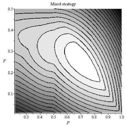
Figure 3. Profit rate from the mixed strategy as a function of sniping threshold $p$ and infinite bid order location $P$.

5.3. Competition between traders.

Finally we comment on the situation that arises when multiple traders compete using the simple strategies described in Section 5.2.

Consider first the case of two competing traders, the first of whom has the ability to employ a sniping strategy of the form described in Section 5.2.2, and the second of whom cannot act quickly enough to snipe but does have the capacity to employ a market making strategy of the form described in Section 5.2.1. Suppose then the market maker places an infinite number of bid, respectively ask, orders at $P$, respectively $1-P$, where $P\leq 1/2$. And suppose the sniper immediately buys every bid that joins the LOB at price above $q$, and every ask that joins the LOB at price below $1-q$, where $P\leq q\leq 1/2$.

For given $P$ and $q$ the behavior of the LOB is as analyzed in Section 5.2.3: but incentives for the two traders are different. Given $P$ and $q$ the profit rate for the sniper is $\int_{P}^{q}(1-2x)\ln(ex/q)dx$ and for the market maker $(1-2P)P\int_{q/e}^{P}1/x\ dx=(1-2P)P\log(eP/q)$ provided $P>\kappa_{b}=q/e$. If $P<q/e$ the market maker’s orders are outside of the recurrent range $(\kappa_{b},1-\kappa_{b})$ of the LOB and so are not matched. It is natural to suppose the sniper follows the market maker: that is the sniper observes the choice $P$ of the market maker and chooses $q$ accordingly. The maximizing choice for the sniper is then $q=\sqrt{P(1-P)}$. Given this, the optimum choice for the market maker, that maximizes his profit rate, is $P\approx 0.340$. At this equilibrium, the profit rate of the market maker is 0.073 and of the sniper 0.020.

Consider next the case of two or more traders using either the market making strategies of Section 5.2.1 or the mixed strategies of Section 5.2.3. Each trader will have an incentive to improve slightly the prices at which she places infinite orders of bids and asks, thus gaining all the profit from those orders for herself alone. The Nash equilibrium has the traders compete away the bid-ask spread and with it all their profits. The model becomes an example of the Bertrand model of price competition and, as there, the conclusion is softened with more realistic assumptions on, for example, capacity constraints or cost asymmetries.

Next consider competition between two or more traders using the sniping strategies of Section 5.2.2; for example between traders who attempt to snipe a limit order as it arrives with an exactly matching limit order. If multiple traders attempt to simultaneously snipe the arriving order, than one of them will succeed and the others will cancel their own orders immediately as they detect that their orders have not been successful. There is clearly an advantage for a trader who can snipe an arriving order more quickly than the other traders, and indeed such a trader can enforce the optimum sniping strategy of Section 5.2.2 and exclude slower traders from the market. It has been argued that competition on speed is wasteful (see [3]), and there are proposals to encourage traders to compete on price, rather than speed, as for example in the proposal of [4] where a market continuous in time is replaced with frequent batch auctions, held perhaps several times a second. We shall explore the consequences of competition on price between sniping traders who can all react at the same speed to a new order entering the LOB.

In such a competitive environment traders will have an incentive to increase the price $q$ above which they snipe bids, and decrease the price $p$ below which they snipe asks, towards $1/2$: they will refrain from sniping orders on which they would expect to make a loss. At the Nash equilibrium, each trader will snipe at all asks with prices below $1/2$ and at all bids with prices above $1/2$ (getting the order with the same probability as each of the other traders). The rightmost bid will then have density $1/x$ on $(1/(2e),1/2)$ by Remark 5. This results in a combined profit rate $1/(2e)-(1+e^{2})/(8e^{2})\approx 0.042$. Thus price competition between sniping traders has decreased their combined profit rate only slightly, from $0.060$ to $0.042$. Alternatively, one can view this reduction as the effect of a batch rather than a continuous market.

Next we comment on the impact of traders on the bid-ask spread. The mean of the distribution (2) can be calculated and is simply $(1-\kappa)/2$. Thus without traders the mean spread between the highest bid and the lowest ask in the LOB is $\kappa\approx 0.218$, while the maximum spread is $1-2\kappa\approx 0.564$. At the Nash equilibrium between sniping traders both are increased, the mean spread to $1/e\approx 0.368$ and the maximum spread to $1-1/e\approx 0.632$. For comparison, with a single sniping trader both are further increased, the mean spread to $1-2(e-1)/(e^{2}+1)\approx 0.590$ and the maximum spread to $1-2/(e^{2}+1)\approx 0.762$; and at the equilibrium between a market making trader and a sniping trader the mean and maximum spread are as low as 0.228 and 0.320 respectively. These calculations are of course for a specific example, but they do illustrate the tractability of the model and its insights.

As a final remark we comment on the inventory of traders under the Nash equilibrium between sniping traders described above. Observe that the LOB below $1/2$ evolves independently of the LOB above $1/2$, and both processes are positive recurrent inside their corresponding thresholds. Consider the net position of the traders collectively, that is all the bids they have matched minus all the asks they have matched, observed at those times when the LOB is empty. This evolves as a symmetric random walk, and is null recurrent. Slight variations of the traders’ strategies would moderate this conclusion: for example, a trader might refrain from sniping bids close enough to $1/2$ when his net position is large. And of course such variations will be essential over longer time-scales than those considered in this paper where the arrival price distributions may vary.

References

- [1] I. Adan and G. Weiss. Exact FCFS matching rates for two infinite multitype sequences. Operations Research, 60:475–489, 2012.
- [2] M. Bramson. Stability and Heavy Traffic Limits for Queueing Networks: St. Flour Lectures Notes. Springer, 2006. http://www.math.duke.edu/~rtd/CPSS2007/Bramson.pdf.
- [3] E. Budish, P. Cramton, and J. Shim. The high-frequency trading arms race: Frequent batch auctions as a market design response. http://faculty.chicagobooth.edu/eric.budish/research/HFT-FrequentBatchAuctions.pdf, 2013.
- [4] E. Budish, P. Cramton, and J. Shim. Implementation details for frequent batch auctions: Slowing down markets to the blink of an eye. American Economic Review, 104:418––424, 2014.
- [5] R. Cont and A. de Larrard. Price dynamics in a markovian limit order book market. SIAM Journal of Financial Mathematics, 4:1–25, 2013.
- [6] R. Cont, S. Stoikov, and R. Talreja. A stochastic model for order book dynamics. Operations Research, 58:549––563, 2010.
- [7] D. Duffie and H. Zhu. Size discovery. NBER Working Paper No. 21696, 2015. http://dx.doi.org/10.3386/w21696.
- [8] D. Easley, M. L. de Prado, and M. O’Hara. The volume clock: Insights into the high frequency paradigm. The Journal of Portfolio Management, 39:19–29, 2012.
- [9] D. Gamarnik and D. Katz. The stability of the deterministic Skorokhod problem is undecidable. Queueing Systems, pages 1–29, 2014.
- [10] X. Gao, J. G. Dai, A. B. Dieker, and S. J. Deng. Hydrodynamic limit of order book dynamics. http://arxiv.org/pdf/1411.7502.pdf, 2014.
- [11] M. D. Gould, M. A. Porter, S. Williams, M. McDonald, D. J. Fenn, and S. D. Howison. Limit order books. Quantitative Finance, 13:1709–1742, 2013.
- [12] D. Kendall. Some problems in the theory of queues. Journal of the Royal Statistical Society, 13(2):151–185, 1951.
- [13] A. Lachapelle, J.-M. Lasry, C.-A. Lehalle, and P.-L. Lions. Efficiency of the price formation process in presence of high frequency participants: a mean field game analysis. http://arxiv.org/pdf/1305.6323v3.pdf, 2014.
- [14] P. Lakner, J. Reed, and F. Simatos. Scaling limit of a limit order book model via the regenerative characterization of Lévy trees. arXiv preprint arXiv:1312.2340, 2013.
- [15] P. Lakner, J. Reed, and S. Stoikov. High frequency asymptotics for the limit order book. Submitted, 2013. http://people.stern.nyu.edu/jreed/Papers/LimitFinal.pdf.
- [16] H. Luckock. A steady-state model of the continuous double auction. Quantitative Finance, 3(5):385–404, 2003.
- [17] C. Maglaras, C. C. Moallemi, and H. Zheng. Queueing dynamics and state space collapse in fragmented limit order book markets. Columbia Business School Research Paper No. 14-13, 2014. http://dx.doi.org/10.2139/ssrn.2403884.
- [18] S. Meyn and R. L. Tweedie. Markov Chains and Stochastic Stability. Cambridge University Press, second edition, 2009.
- [19] J. Plačková. Shluky volatility a dynamika poptávky a nabídky. Master Thesis, MFF, Charles University Prague, 2011. (In Czech).
- [20] I. Roşu. A dynamic model of the limit order book. Review of Financial Studies, 22:4601–4641, 2009.
- [21] F. Simatos. Coupling limit order books and branching random walks. Journal of Applied Probability, 51:625–639, 2014.
- [22] G. Stigler. Public regulation of the securities markets. The Journal of Business, 37(2):117–142, 1964.
- [23] A. L. Stolyar and E. Yudovina. Systems with large flexible server pools: Instability of “natural” load balancing. Annals of Applied Probability, 23:2099–2138, 2013.
- [24] J. Swart. Rigorous results for the stigler-luckock model for the evolution of an order book. Submitted, 2016. arXiv:1605.01551.
- [25] M. Toke. The order book as a queueing system: average depth and influence of the size of limit orders. Quantitative Finance, 14, 2014.
- [26] E. Yudovina. Collaborating Queues: Large Service Network and a Limit Order Book. Ph.D. thesis, University of Cambridge, 2012.
- [27] S. A. Zenios, G. M. Chertow, and L. M. Wein. Dynamic allocation of kidneys to candidates on the transplant waiting list. Operations Research, 48:549–569, 2000.