Method for an unbinned measurement of the $q^{2}$ dependent decay amplitudes of $\kern 2.59189pt\overline{\kern-2.59189ptB}{}^{0}\!\rightarrow\kern 2.87996pt\overline{\kern-2.87996ptK}{}^{*0}\mu^{+}\mu^{-}$ decays

U. Egede¹, M. Patel¹, K.A. Petridis^2,1

¹Imperial College London, London, United Kingdom
²Univeristy of Bristol, Bristol, United Kingdom

A method for determining the $q^{2}$ dependent $\kern 1.99997pt\overline{\kern-1.99997ptK}{}^{*0}$ spin amplitudes of $\kern 1.79993pt\overline{\kern-1.79993ptB}{}^{0}\!\rightarrow\kern 1.99997pt\overline{\kern-1.99997ptK}{}^{*0}\mu^{+}\mu^{-}$ decays through a maximum likelihood fit to data is presented. While current experimental techniques extract a limited set of observables in bins of $q^{2}$, our approach allows for the determination of all observable quantities as continuous distributions in $q^{2}$. By doing this, the method eliminates the need to correct theory predictions of these observables for $q^{2}$ averaging effects, thus increasing the sensitivity to the effects of physics beyond the Standard Model. Accounting for the symmetries of the angular distribution and using a three parameter ansatz for the $q^{2}$ dependence of the amplitudes, the precision of the angular observables and the sensitivity to new physics is estimated using simulated events. These studies are based on the sample sizes collected by the LHCb experiment during Run-I and expected for Run-II.

 

1 Introduction

Rare $b\rightarrow s\mu^{+}\mu^{-}$ processes are suppressed in the Standard Model (SM) as they can proceed only via electroweak penguin or box type diagrams. As-yet undiscovered particles could give additional contributions with comparable amplitudes to those of the SM processes, and such decays are therefore sensitive probes of new phenomena.

The angular distribution of the $K^{-}\pi^{+}\mu^{+}\mu^{-}$ system in $\kern 1.79993pt\overline{\kern-1.79993ptB}{}^{0}\!\rightarrow\kern 1.99997pt\overline{\kern-1.99997ptK}{}^{*0}\mu^{+}\mu^{-}$ decays is of particular interest, as it can be described by a number of measurable quantities which are sensitive to new physics and can be precisely predicted in a given physics model. Theoretical predictions for such observables are particularly precise in the range of dimuon invariant mass squared, $q^{2}$, $1<q^{2}<6~{}{\mathrm{\,Ge\kern-1.00006ptV^{2}\!/}c^{4}}$ [1, 2, 3, 4, 5, 6, 7, 8]. The potential of the $\kern 1.79993pt\overline{\kern-1.79993ptB}{}^{0}\!\rightarrow\kern 1.99997pt\overline{\kern-1.99997ptK}{}^{*0}\mu^{+}\mu^{-}$ decay as a probe of New Physics (NP) has resulted in numerous proposals for observables with varying levels of theoretical precision, as described in Refs. [9, 10, 11, 1, 12, 13, 14].

The dominant uncertainty in the predictions of $\kern 1.79993pt\overline{\kern-1.79993ptB}{}^{0}\!\rightarrow\kern 1.99997pt\overline{\kern-1.99997ptK}{}^{*0}\mu^{+}\mu^{-}$ observables, is attributed to the calculation of the $\kern 1.79993pt\overline{\kern-1.79993ptB}{}^{0}\rightarrow\kern 1.99997pt\overline{\kern-1.99997ptK}{}^{*0}$ hadronic form-factors. The LHCb collaboration have determined a number of observables which are designed to have a reduced dependence on these form-factors [15, 16]. The measurement of the observable $P_{5}^{\prime}$ [13], which is designed to ensure the cancellation of the hadronic $\kern 1.79993pt\overline{\kern-1.79993ptB}{}^{0}\rightarrow\kern 1.99997pt\overline{\kern-1.99997ptK}{}^{*0}$ soft form-factors at leading order, exhibits a local tension at the level of 3.7 $\sigma$ with respect to the SM prediction of Ref [13]. This measurement has been interpreted as an indication of a new, heavy, vector particle [17, 18, 19, 20, 21, 22, 23, 24, 25, 26, 27, 6, 28, 29] or as a consequence of previously unaccounted for QCD effects [30, 31, 32]. In addition to potentially unexpected QCD effects, there are several other factors that limit the sensitivity of the data to new physics effects. As detailed below, these include the omission of certain symmetry relations between the observables in experimental analyses, the interference between P- and S-waves of the $K^{-}\pi^{+}$ system, and the binning in $q^{2}$.

The LHCb collaboration have published a number of separate analyses of $\kern 1.79993pt\overline{\kern-1.79993ptB}{}^{0}\!\rightarrow\kern 1.99997pt\overline{\kern-1.99997ptK}{}^{*0}\mu^{+}\mu^{-}$ decays to determine different observables [33, 15]. Recently, the LHCb collaboration also presented a measurement of all observables related to the $K^{-}\pi^{+}$ system in a P-wave state [16]. In all these measurements, the simple relations between the P-wave observables, arising due to the symmetries of the angular distribution, are implemented. However, the remaining complex relation between P-wave observables [11, 34], is not exploited. This results in redundant parameters being determined, reducing the overall experimental precision of the observables.

One of the dominant systematic uncertainties for the experimental determination of $\kern 1.79993pt\overline{\kern-1.79993ptB}{}^{0}\!\rightarrow\kern 1.99997pt\overline{\kern-1.99997ptK}{}^{*0}\mu^{+}\mu^{-}$ observables is the lack of knowledge of the S-wave contribution to the predominately P-wave $K^{-}\pi^{+}$ system. An S-wave contribution can induce a bias on the (P-wave) observables and dilute the experimental sensitivity to such observables [35]. Until recently, the experimental results included a systematic uncertainty to cover this. In the latest LHCb analysis [16], the S-wave components are explicitly included. However, further symmetry relations between the P- and S-wave components are not accounted for, resulting in two redundant S-wave parameters [36]. As in the case of the omitted P-wave symmetry relations, this redundancy dilutes the experimental precision of the observables of the angular distribution.

The precision of global fits to existing measurements of $\kern 1.79993pt\overline{\kern-1.79993ptB}{}^{0}\!\rightarrow\kern 1.99997pt\overline{\kern-1.99997ptK}{}^{*0}\mu^{+}\mu^{-}$ transitions are also limited by the fact that the measurements are performed in bins in $q^{2}$. Comparison between theoretical predictions and experimental measurements then requires the integration of theoretically predicted observables over experimental $q^{2}$ bins. This integration has the effect of diluting variations and introducing dependence on other, potentially more poorly predicted, observables. For example, the angular terms in the differential decay rate that involve the theoretically clean $P_{5}^{\prime}$ observable have a $\sqrt{F_{\rm L}(1-F_{\rm L})}$ prefactor, where $F_{\rm L}$ is the longitudinal polarisation fraction of the $\kern 1.99997pt\overline{\kern-1.99997ptK}{}^{*0}$ and is a poorly predicted observable. This results in the experimental measurements being sensitive to, $\int{\sqrt{F_{\rm L}(q^{2})(1-F_{\rm L}(q^{2}))}}P_{5}^{\prime}(q^{2})dq^{2}$. Although the angular distribution is also sensitive to $\int{F_{\rm L}(q^{2})dq^{2}}$, this does not enable $\int{P_{5}^{\prime}(q^{2})dq^{2}}$ to be computed and hence does not allow the full exploitation of the cancellation of the form factors at leading order for which $P_{5}^{\prime}$ was designed.

In this paper, we propose a method of analysing $\kern 1.79993pt\overline{\kern-1.79993ptB}{}^{0}\!\rightarrow\kern 1.99997pt\overline{\kern-1.99997ptK}{}^{*0}\mu^{+}\mu^{-}$ decays that allows the determination of all of the $\kern 1.99997pt\overline{\kern-1.99997ptK}{}^{*0}$ amplitudes as a parametric function of $q^{2}$. This method allows the formation of any observable from a single fit to the data from a given experiment, including the full experimental correlations. The method also allows the S-wave related amplitudes to be determined, removing the need for any experimental systematic uncertainty from S-wave contamination. The $q^{2}$ shape information and the application of all the symmetry relations of the angular distribution, result in a substantial gain in sensitivity to new physics effects and completely remove the $q^{2}$ averaging problem mentioned above. The method can be used with the $\kern 1.79993pt\overline{\kern-1.79993ptB}{}^{0}\!\rightarrow\kern 1.99997pt\overline{\kern-1.99997ptK}{}^{*0}\mu^{+}\mu^{-}$ sample that is already available at the LHCb experiment.

The paper is organised as follows: Sec. 2 describes the decay rate and angular observables of $\kern 1.79993pt\overline{\kern-1.79993ptB}{}^{0}\!\rightarrow K^{-}\pi^{+}\mu^{+}\mu^{-}$ transitions; Sec. 3 describes the method for extracting the $\kern 1.99997pt\overline{\kern-1.99997ptK}{}^{*0}$ helicity amplitudes from a single fit to data; Sec. 4 presents the results of the method using simulated $\kern 1.79993pt\overline{\kern-1.79993ptB}{}^{0}\!\rightarrow\kern 1.99997pt\overline{\kern-1.99997ptK}{}^{*0}\mu^{+}\mu^{-}$ decays with sample sizes equivalent to those obtained by LHCb during Run-I and projected for Run-II of the LHC; finally Sec. 5 compares the sensitivity of the amplitude fit to other methods for extracting the $\kern 1.99997pt\overline{\kern-1.99997ptK}{}^{*0}$ angular observables.

2 The differential decay rate

The differential decay rate of the $\kern 1.79993pt\overline{\kern-1.79993ptB}{}^{0}$ meson, for a $K\pi$ system in a P-wave configuration and ignoring scalar contributions to the dimuon system, is given by [9]

$$\frac{\mathrm{d}^{4}\Gamma[\kern 1.79993pt\overline{\kern-1.79993ptB}{}^{0}\!\rightarrow\kern 1.99997pt\overline{\kern-1.99997ptK}{}^{*0}\mu^{+}\mu^{-}]}{\mathrm{d}\cos\theta_{\ell}\,\mathrm{d}\cos\theta_{K}\,\mathrm{d}\phi\,\mathrm{d}q^{2}}= \frac{9}{32\pi}[\frac{}{}{J_{1s}}\sin^{2}\theta_{K}+{J_{1c}}\cos^{2}\theta_{K}+{J_{2s}}\sin^{2}\theta_{K}\cos 2\theta_{\ell}~{}+$$

$$\phantom{\frac{9}{32\pi}}~{}\frac{}{}{J_{2c}}\cos^{2}\theta_{K}\cos 2\theta_{\ell}+{J_{3}}\sin^{2}\theta_{K}\sin^{2}\theta_{\ell}\cos 2\phi~{}+$$

$$\phantom{\frac{9}{32\pi}}~{}\frac{}{}{J_{4}}\sin 2\theta_{K}\sin 2\theta_{\ell}\cos\phi+{J_{5}}\sin 2\theta_{K}\sin\theta_{\ell}\cos\phi~{}+$$ (1)

$$\phantom{\frac{9}{32\pi}}~{}\frac{}{}{J_{6s}}\sin^{2}\theta_{K}\cos\theta_{\ell}+{J_{7}}\sin 2\theta_{K}\sin\theta_{\ell}\sin\phi~{}+$$

$$\phantom{\frac{9}{32\pi}}~{}\frac{}{}{J_{8}}\sin 2\theta_{K}\sin 2\theta_{\ell}\sin\phi+{J_{9}}\sin^{2}\theta_{K}\sin^{2}\theta_{\ell}\sin 2\phi\frac{}{}].$$

The angular observables, $J_{i}(q^{2})$, depend on six $q^{2}$ dependent complex amplitudes, $A_{0}^{L,R}$, $A_{\parallel}^{L,R}$, $A_{\perp}^{L,R}$ representing the three polarisation states of the $\kern 1.99997pt\overline{\kern-1.99997ptK}{}^{*0}$. The configuration of a longitudinally polarised $K^{*0}$ and time-like polarised dimuon system is suppressed and therefore safely neglected. The labels $L$ and $R$ refer to the chirality of the dimuon system. The various $J_{i}(q^{2})$ observables are given by

$$\begin{split}J_{1s}&=\frac{(2+\beta_{\mu}^{2})}{4}\bigl{[}|A_{\perp}^{L}|^{2}+|A_{\parallel}^{L}|^{2}+(L\rightarrow R)\bigr{]}+\frac{4m_{\mu}^{2}}{q^{2}}\mathrm{Re}(A_{\perp}^{L}A_{\perp}^{R*}+A_{\parallel}^{L}A_{\parallel}^{R*})\\ J_{1c}&=|A_{0}^{L}|^{2}+|A_{0}^{R}|^{2}+\frac{4m_{\mu}^{2}}{q^{2}}\bigl{[}2\mathrm{Re}(A_{0}^{L}A_{0}^{R*})\bigr{]}\\ J_{2s}&=\frac{\beta_{\mu}^{2}}{4}\biggl{[}|A_{\perp}^{L}|^{2}+|A_{\parallel}^{L}|^{2}+(L\rightarrow R)\biggr{]}\\ J_{2c}&=-\beta_{\mu}^{2}\biggl{[}|A_{0}^{L}|^{2}+(L\rightarrow R)\biggr{]}\\ J_{3}&=\frac{\beta_{\mu}^{2}}{2}\biggl{[}|A_{\perp}^{L}|^{2}-|A_{\parallel}^{L}|^{2}+(L\rightarrow R)\biggr{]}\\ J_{4}&=\frac{\beta_{\mu}^{2}}{\sqrt{2}}\biggl{[}\mathrm{Re}(A_{0}^{L}A_{\parallel}^{L*})+(L\rightarrow R)\biggr{]}\\ J_{5}&=\sqrt{2}\beta_{\mu}\biggl{[}\mathrm{Re}(A_{0}^{L}A_{\perp}^{L*})-(L\rightarrow R)\biggr{]}\\ J_{6s}&=2\beta_{\mu}\biggl{[}\mathrm{Re}(A_{\parallel}^{L}A_{\perp}^{L*})-(L\rightarrow R)\biggr{]}\\ J_{7}&=\sqrt{2}\beta_{\mu}\biggl{[}\mathrm{Im}(A_{0}^{L}A_{\parallel}^{L*})-(L\rightarrow R)\biggr{]}\\ J_{8}&=\frac{\beta_{\mu}^{2}}{\sqrt{2}}\biggl{[}\mathrm{Im}(A_{0}^{L}A_{\perp}^{L*})+(L\rightarrow R)\biggr{]}\\ J_{9}&=\beta_{\mu}^{2}\biggl{[}\mathrm{Im}(A_{\parallel}^{L*}A_{\perp}^{L})+(L\rightarrow R)\biggr{]}\end{split}$$ (2)

with $\beta_{\mu}^{2}=(1-4m_{\mu}^{2}/q^{2})$ and $(L\rightarrow R)$ denotes the same term but with flipped chirality. In the limit of $q^{2}\gg 4m_{\mu}^{2}$ the various $J_{i}$ coefficients can be trivially related by $J_{2c}=-J_{1c}$ and $J_{2s}=J_{1s}/3$. An additional, more complicated relation exists between $J_{2c}$ and the rest of the angular observables as noted in Ref. [11] and explicitly given in Ref. [34].

While the differential decay rate in Eq. 1 is defined for the decay of the $\kern 1.79993pt\overline{\kern-1.79993ptB}{}^{0}$ meson, the decay of the $B^{0}$ can be given in complete analogy, by starting from Eq. 1 and performing the substitution $J_{i}\rightarrow\bar{J}_{i}$, following the angular convention described in Refs. [33, 15] This convention allows the sum of the decay rates of $B^{0}$ and $\kern 1.79993pt\overline{\kern-1.79993ptB}{}^{0}$ mesons to be written in terms of sums of $J_{i}$ and $\bar{J}_{i}$ angular observables by simply performing the substitutions $J_{i}\rightarrow(\bar{J}_{i}+J_{i})$ into Eq. (1). It is therefore convenient to define $C\!P$-averaged observables $S_{i}$, as discussed in Ref. [1],

$$S_{i} \equiv\frac{J_{i}+\bar{J}_{i}}{\left({\rm d}\Gamma+{\rm d}\bar{\Gamma}\right)/{\rm d}q^{2}}.$$ (3)

In a similar way, the $C\!P$-asymmetric observables, $A_{i}$, are defined as [1]

$$A_{i} \equiv\frac{J_{i}-\bar{J}_{i}}{\left({\rm d}\Gamma+{\rm d}\bar{\Gamma}\right)/{\rm d}q^{2}}.$$ (4)

2.1 S-wave interference

The expression in Eq. (1) assumes that the $K^{-}\pi^{+}$ system is in a P-wave configuration, as is the case for the $K^{*0}(892)$ vector meson. To account for a $K^{-}\pi^{+}$ system in an S-wave configuration, the spin-amplitudes need to be modified to account for the presence of the S-wave amplitudes $A_{00}^{L,R}$.

In previous experimental analyses [33, 15] the presence of an S-wave contribution was accounted for by assigning a systematic uncertainty. The method presented here enables the determination of the S-wave amplitudes using a modified version of Eq. 1,

$$\begin{split}\frac{\mathrm{d}^{4}\Gamma}{\mathrm{d}\cos\theta_{\ell}\,\mathrm{d}\cos\theta_{K}\,\mathrm{d}\phi\,\mathrm{d}q^{2}}~{}\rightarrow~{}&\frac{\mathrm{d}^{4}\Gamma}{\mathrm{d}\cos\theta_{\ell}\,\mathrm{d}\cos\theta_{K}\,\mathrm{d}\phi\,\mathrm{d}q^{2}}~{}+\\ \frac{9}{32\pi}[~{}{J^{\prime}}_{1c}(1-\cos 2\theta_{\ell})~{}+&{J^{\prime\prime}}_{1c}\cos\theta_{K}(1-\cos 2\theta_{\ell})~{}+\\ \phantom{\frac{9}{32\pi}[}~{}{J^{\prime}}_{4}\sin 2\theta_{\ell}\sin\theta_{K}\cos\phi~{}+&{J^{\prime}}_{5}\sin\theta_{\ell}\sin\theta_{K}\cos\phi~{}+\\ \phantom{\frac{9}{32\pi}[}~{}{J^{\prime}}_{7}\sin\theta_{\ell}\sin\theta_{K}\sin\phi~{}+&{J^{\prime}}_{8}\sin 2\theta_{\ell}\sin\theta_{K}\sin\phi~{}],\end{split}$$ (5)

with

$$\begin{split}{J^{\prime}}_{1c}&=\frac{1}{3}|A_{00}^{L}|^{2}+\frac{1}{3}|A_{00}^{R}|^{2}\\ {J^{\prime\prime}}_{1c}&=\frac{2}{\sqrt{3}}\biggl{[}\mathrm{Re}(A_{00}^{L}A_{0}^{L*})+(L\rightarrow R)\biggr{]}\\ {J^{\prime}}_{4}&=\sqrt{\frac{2}{3}}\biggl{[}\mathrm{Re}(A_{00}^{L}A_{\parallel}^{L*})+(L\rightarrow R)\biggr{]}\\ {J^{\prime}}_{5}&=2\sqrt{\frac{2}{3}}\biggl{[}\mathrm{Re}(A_{00}^{L}A_{\perp}^{L*})-(L\rightarrow R)\biggr{]}\\ {J^{\prime}}_{7}&=2\sqrt{\frac{2}{3}}\biggl{[}\mathrm{Im}(A_{00}^{L}A_{\parallel}^{L*})-(L\rightarrow R)\biggr{]}\\ {J^{\prime}}_{8}&=\sqrt{\frac{2}{3}}\biggl{[}\mathrm{Im}(A_{00}^{L}A_{\perp}^{L*})+(L\rightarrow R)\biggr{]},\\ \end{split}$$ (6)

as given in Ref. [14], where an implicit integration over the mass of the $K^{-}\pi^{+}$ system is assumed.

The fraction of the S-wave contribution is defined as:

$$F_{\rm S}(q^{2})=\frac{|A_{00}^{L}|^{2}+|A_{00}^{R}|^{2}}{\mathrm{d}\Gamma/\mathrm{d}q^{2}}$$ (7)

Where $\mathrm{d}\Gamma/\mathrm{d}q^{2}$ is defined as the total differential rate of both S and P-wave contributions, given by

$$\begin{split}\frac{\mathrm{d}\Gamma}{\mathrm{d}q^{2}}&=\frac{\mathrm{d}\Gamma_{\rm S}}{\mathrm{d}q^{2}}+\frac{\mathrm{d}\Gamma_{\rm P}}{\mathrm{d}q^{2}}\\ &=|A_{00}^{L}|^{2}+|A_{0}^{L}|^{2}+|A_{\parallel}^{L}|^{2}+|A_{\perp}^{L}|^{2}+(L\rightarrow R).\\ \end{split}$$ (8)

3 Fitting for the ${\boldsymbol{K^{*0}}}$ amplitudes

3.1 Infinitesimal symmetries of the angular distribution

Ignoring the S-wave terms, the angular distribution of $\kern 1.79993pt\overline{\kern-1.79993ptB}{}^{0}\!\rightarrow\kern 1.99997pt\overline{\kern-1.99997ptK}{}^{*0}\mu^{+}\mu^{-}$ decays can be described by eleven angular observables ($J_{i}$) for each $B^{0}$ flavour. These observables are made up of bilinear combinations of the $K^{*0}$ spin amplitudes and represent the “experimental” degrees of freedom. If the $J_{i}$ terms are all independent, the experimental degrees of freedom should match the number of amplitude components which represent the “theoretical” degrees of freedom. However, there are continuous symmetry transformations of the amplitudes that leave the decay rate invariant [11]. In order for the degrees of freedom to match it is required that

$$n_{j}-n_{d}=2n_{a}-n_{s},$$ (9)

where $n_{j}$ is the number of $J_{i}$ terms, $n_{d}$ the number of the relations between the $J_{i}$, $n_{a}$ is the number of complex amplitude components and $n_{s}$ is a number of continuous symmetry transformations of the amplitudes that leave the decay rate invariant. In the massless limit $(q^{2}\gg 4m_{\mu}^{2})$, and ignoring scalar contributions to the dimuon system, there are four continuous symmetry transformations of the amplitudes ($n_{s}=4$) that leave each of the $J_{i}$, and therefore the decay rate invariant, (see [11, 34] for a detailed discussion). Given $n_{j}=11$ and $n_{a}=12$, as specified by Eq. 9, there are three relations between the various $J_{i}$, yielding eight independent angular observables.

The following continuous transformations of the amplitudes, leave the angular distribution unchanged [11, 34]:

$$n^{\prime}_{i}=\left(\begin{array}[]{cc}{\color[rgb]{0,0,0}e^{i\phi_{L}}}&0\\ 0&{\color[rgb]{0,0,0}e^{-i\phi_{R}}}\end{array}\right)\left({\color[rgb]{0,0,0}\begin{array}[]{cc}\cos\theta&-\sin\theta\\ \sin\theta&\cos\theta\end{array}}\right)\left({\color[rgb]{0,0,0}\begin{array}[]{cc}\cosh i\omega&-\sinh i\omega\\ -\sinh i\omega&\cosh i\omega\end{array}}\right)n_{i}~{},$$ (10)

where the basis vectors $n_{i}$ are defined as,

$$n_{\parallel}=\left(\begin{array}[]{c}A_{\parallel}^{L}\\ A_{\parallel}^{R*}\end{array}\right)~{},~{}n_{\perp}=\left(\begin{array}[]{c}A_{\perp}^{L}\\ -A_{\perp}^{R*}\end{array}\right)~{},~{}n_{0}=\left(\begin{array}[]{c}A_{0}^{L}\\ A_{0}^{R*}\end{array}\right),$$ (11)

The components $\phi_{L}$ and $\phi_{R}$ are phase-rotations of the left- and right-handed amplitudes separately. The second and third matrices act as a transformation between the left- and right-handed amplitudes.

The angular distribution is degenerate under these transformations of the amplitudes. A likelihood function including all twelve real amplitude components, would therefore exhibit a 4D hypersurface of continuous maxima in amplitude space, rendering useless the minimisation techniques for the determination of the amplitude components. The symmetries of the angular distribution allow for the transformation of the amplitudes to a particular basis, where four of the amplitude components are fixed to some arbitrary value at every point in $q^{2}$. The choice of the basis, referred to as “basis-fixing”, lifts the degeneracy. For the basis-fixing to allow for a subsequent fit of the remaining eight amplitudes as a function of $q^{2}$, it is required that the values for $\phi_{L}$, $\phi_{R}$, $\theta$, and $\omega$ exist for every point in $q^{2}$; and the amplitudes in this transformed basis are slowly varying in $q^{2}$, such that they can be described by a simple functional form. This second requirement restricts the $q^{2}$ range where the amplitudes can be extracted. The presence of potential light resonances below $\sim 1$ ${\mathrm{\,Ge\kern-1.00006ptV^{2}\!/}c^{4}}$ and of $c\bar{c}$ resonances above 8 ${\mathrm{\,Ge\kern-1.00006ptV^{2}\!/}c^{4}}$ motivates the use of the resonance-free and theoretically preferred region of $1<q^{2}<6$ ${\mathrm{\,Ge\kern-1.00006ptV^{2}\!/}c^{4}}$.

A previous study described in Ref. [11] used the following basis-fixing

$$\mathrm{Re}(A_{\parallel}^{L})=\mathrm{Im}(A_{\parallel}^{L})=\mathrm{Im}(A_{\parallel}^{R})=\mathrm{Im}(A_{\perp}^{R})=0.$$ (12)

This basis suffers from a rapidly varying behaviour in $\mathrm{Im}(A_{0}^{L})$ at $q^{2}\sim 2{\mathrm{\,Ge\kern-1.00006ptV^{2}\!/}c^{4}}$, as shown in Fig. 1. In Ref. [11], the problems caused by this discontinuity were avoided by ignoring the $q^{2}$ region below 2.5${\mathrm{\,Ge\kern-1.00006ptV^{2}\!/}c^{4}}$.

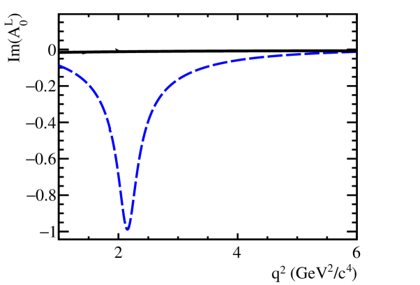
Figure 1: Distribution of the SM $\mathrm{Im}(A_{0}^{L})$ amplitude in the untransformed (solid black) and in the fixed-basis proposed in Ref. [11] (dashed blue). The untransformed amplitudes are given by the EOS program [3], up to an overall scaling factor.

Ignoring the $q^{2}$ region below 2.5${\mathrm{\,Ge\kern-1.00006ptV^{2}\!/}c^{4}}$ is clearly highly undesirable. For the method that we propose here, we instead use,

$$\mathrm{Re}(A_{0}^{R})=\mathrm{Im}(A_{0}^{R})=\mathrm{Im}(A_{0}^{L})=\mathrm{Im}(A_{\perp}^{R})=0.$$ (13)

The amplitudes in the improved fixed-basis then exhibit a slow varying behaviour in $q^{2}$ both in the SM, shown in Fig. 2 as well as in a range of new physics models. The EOS program [3] is used to generate the amplitudes in the original basis.

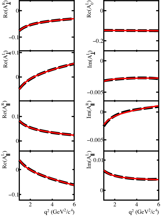
Figure 2: Distribution of the transformed SM $K^{*0}(892)$ spin amplitudes in the fixed-basis (dashed black line) which exhibit a smooth behaviour in $q^{2}$. The solid red line denotes the result of the fit of the $q^{2}$ dependent ansatz discussed in the Sec. 3.3. The untransformed amplitudes are given by the EOS program [3], up to an overall scaling factor. Only the non-zero amplitude components in the fixed-basis are shown.

3.2 Exact discrete symmetries

In addition to the continuous transformations of the amplitudes that leave the angular distribution invariant, the angular distribution is also invariant under discrete transformations of the amplitudes. Even after the basis-fixing, which reduces the number of amplitudes to eight, there is a discrete symmetry comprising a simultaneous shift $A_{i}\rightarrow-A_{i}$ for all $i$, that leaves the angular distribution invariant. This symmetry can be seen simply by inspecting Eq. 2 and noting that even after the conditions of Eq. 13 have been applied, all angular observables are still constructed out of products of spin-amplitudes in the fixed-basis.

3.3 Approximate discrete symmetries

The limited amount of signal candidates available in the experimental data, can give rise to approximate symmetries under discrete transformations of the amplitudes. The exact form of these approximate symmetries can depend on the basis-fixing transformations discussed in Sec. 3.1. Given the basis-fixing condition of Eq. (13), a clear example occurs in the transformed basis with the SM amplitudes, where the lack of right-handed currents can give rise to an approximate symmetry under the transformation

$$A_{\parallel}^{L} \rightarrow-A_{\perp}^{L}$$

$$A_{\perp}^{L} \rightarrow-\frac{A_{\parallel}^{L}}{2}$$ (14)

The effect of this accidental approximate symmetry can be demonstrated by generating samples based on the SM and on a model with large right-handed Wilson coefficients. Figure 3 shows the effect of the discrete transformation of Eq. 3.3 on $\cos\theta_{\ell}$, both in the SM and the model with large right-handed currents. The region where $-\pi/4<\phi<\pi/2$ and $0<\cos\theta_{K}<1$ is considered, in order to reduce possible cancellation of terms arising from the integration of the angular distribution over $\phi$ and $\cos\theta_{K}$. Figure 3 shows that in the SM the angular distribution in $\cos\theta_{\ell}$ is essentially indistinguishable under the transformation; whereas, in the model with right-handed currents, the angular distributions can be distinguished. It is therefore clear that the above transformation is an approximate discrete symmetry of the angular distribution only in the SM and in other models with no right-handed currents.

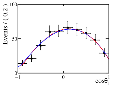
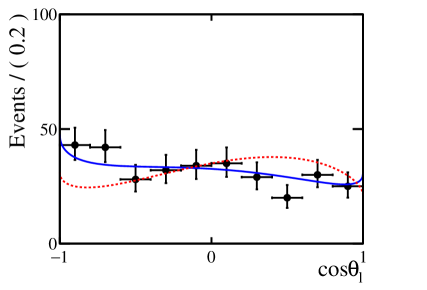
Figure 3: Demonstration of the effect of the transformation of Eq. (3.3) in the SM (left) and in a model with large right-handed Wilson Coefficients (right). The amount of data corresponds to the expected number of $\kern 1.61993pt\overline{\kern-1.61993ptB}{}^{0}\!\rightarrow\kern 1.79997pt\overline{\kern-1.79997ptK}{}^{*0}\mu^{+}\mu^{-}$ candidates in LHCb’s Run-II dataset. The blue line denotes the model that the data is generated from. The red-dashed line denotes the model with the approximate symmetry transformation, as mentioned in the main text, applied. The angles $\phi$ and $\theta_{K}$ are required to satisfy $-\pi/4<\phi<\pi/2$ and $0<\cos\theta_{K}<1$.

An additional approximate discrete symmetry exists under the transformation of the right handed amplitudes in the transformed basis

$$A_{\parallel}^{R} \leftrightarrow-A_{\perp}^{R}.$$ (15)

As for the left-handed amplitudes, the transformation of Eq. (15) is an approximate discrete symmetry of the angular distribution only in the SM and in other models with no right-handed currents.

3.4 Parameterised amplitudes

In order to determine the $q^{2}$ dependent $\kern 1.99997pt\overline{\kern-1.99997ptK}{}^{*0}$ spin amplitudes, a $q^{2}$ parametrisation of the amplitudes in the fixed-basis needs to be employed. A three-parameter ansatz of the form

$$A=\alpha+\beta q^{2}+\gamma/q^{2}$$ (16)

for both the real and imaginary components of each left- and right- handed amplitudes is chosen. No attempt is made to interpret these $\alpha$, $\beta$ and $\gamma$ coefficients in terms of short- or long-distance parameters. The choice of this ansatz is justified by fitting the transformed spin amplitudes, as provided by the EOS program [3], in the SM and numerous other physics models, using the parametrisation described above. Figure 2 shows the result of the SM fit. Any bias coming from this choice of ansatz will be much smaller than the statistical uncertainty of current and any foreseeable-future experimental measurements.

The basis-fixing reduces the number of amplitude components that need to be determined to eight per $B^{0}$ flavour. Considering that each such component is described by three parameters to account for the $q^{2}$ dependence, in total there are twenty-four amplitude parameters per $B^{0}$ flavour that need to be determined. This parameter counting ignores any S-wave amplitudes. Such amplitudes are discussed further in Sec. 3.5. Alternatively, the model dependent assumption can be made, that the only weak phases present in the amplitudes come from the CKM matrix elements. This assumption leads to the $B^{0}$ and $\kern 1.79993pt\overline{\kern-1.79993ptB}{}^{0}$ amplitudes being identical, as the diagrams with non-zero weak phases are Cabibbo suppressed. Accounting for the experimental angular convention of the decay rate described in Sec. 2, the decay distribution of both the $B^{0}$ and $\kern 1.79993pt\overline{\kern-1.79993ptB}{}^{0}$ decays can be described using a single set of amplitude parameters. The approaches with separate and identical $B^{0}$ and $\kern 1.79993pt\overline{\kern-1.79993ptB}{}^{0}$ amplitude parameters, are both discussed below.

3.5 S-wave contribution

Previous studies have discussed both the potential size as well as the impact of the S-wave contribution in the angular analysis of $B^{0}\!\rightarrow K^{*0}\mu^{+}\mu^{-}$ decays [37, 38, 35]. In particular, it has been shown that the number of signal candidates expected in LHCb’s Run-I dataset, ignoring the S-wave contribution can have a significant effect on some angular observables. It is therefore critical that the $q^{2}$ dependent S-wave amplitude components are also accounted for in the fit to the angular distribution of $B^{0}\!\rightarrow K^{*0}\mu^{+}\mu^{-}$ decays.

In this study, the S-wave amplitudes are included in the angular distribution of the signal based on Eq. 5 and are treated as nuisance parameters in the fit. The $K^{+}\pi^{-}$ mass range considered corresponds to 100 ${\mathrm{\,Me\kern-1.00006ptV\!/}c^{2}}$ around the $K^{*0}(892)$ pole mass. The $m_{K\pi}$ dependence is accounted for by modifying each $J_{i}$ term in Eq. 5 by

$$J_{ij}=A_{i}A_{j}^{*}\rightarrow A_{i}A_{j}^{*}\int g_{i}(m_{K\pi})g_{j}^{*}(m_{K\pi})dm_{K\pi},$$ (17)

where $g_{i}(m_{K\pi})$ represents the $m_{K\pi}$ line-shape of either a P-wave or an S-wave amplitude. It is thus assumed that the amplitudes do not explicitly depend on $m_{K\pi}$.

The $q^{2}$ dependence of the S-wave amplitudes used in the generation of the simulated events are calculated following Ref. [39]. For simplicity, only the $\kappa(600)$ is considered to contribute to the S-wave in the $K^{+}\pi^{-}$ mass range considered. This means that for this analysis only the line-shape of the $\kappa$ is considered to contribute to the S-wave $g_{i}(m_{K\pi})$. The line-shape of both the $\kappa(600)$ and the $K^{*0}(892)$ are taken as relativistic Breit-Wigner distributions with mass and width parameters as given in Ref. [40]. The form-factor of the $\kappa(600)$ is taken from Ref. [41]. The values of the corresponding $\int g_{i}(m_{K\pi})g_{j}^{*}(m_{K\pi})dm_{K\pi}$ terms are shown in Tab. 1. In the SM, the resulting value of $F_{S}$ as a function of $q^{2}$ is shown in Fig. 4. Using this simplistic approach, the predicted value of $F_{S}$ is similar to the values obtained using more sophisticated treatments, such as those of Refs. [37, 38].

Given the size of current data samples, and the fact that the S-wave fraction is expected to be small ($\mathcal{O}(10\%)$), the $q^{2}$ dependence of the S-wave amplitudes $A_{00}^{L,R}$, can be approximated to be constant as a function of $q^{2}$ when performing fits to the data. This is a good approximation since the $q^{2}$ shape of the S-wave amplitudes is expected to be similar to that of $A_{0}^{L,R}$ [39], which is approximately constant in the region $1<q^{2}<6$ ${\mathrm{\,Ge\kern-1.00006ptV^{2}\!/}c^{4}}$.

Table 1: Summary of the various integrals of the S- and P- wave line shapes that are used both in this study. The integral is performed in the $m_{K\pi}$ range $[796,996]~{}{\mathrm{\,Ge\kern-1.00006ptV\!/}c^{2}}$.

Term	Value
$\int|g_{K^{*0}}|^{2}dm_{K\pi}$	$0.80$
$\int|g_{\kappa}|^{2}dm_{K\pi}$	$0.18$
$\int g_{\kappa}g_{K^{*0}}^{*}dm_{K\pi}$	$0.22-0.23i$

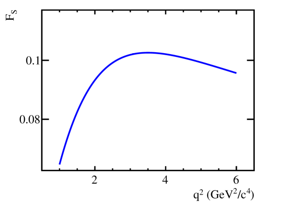
Figure 4: Estimate of the S-wave fraction $F_{S}$ in the SM as a function of $q^{2}$ using the simplistic approach described in the text.

3.6 Determining the amplitudes

The stability and sensitivity of a fit for the $q^{2}$ dependent amplitudes is determined using simulated data with sample sizes equivalent to those expected at LHCb during Run-I and Run-II of the LHC. Estimates of the signal and background yields are taken from Refs. [33, 15] and scaled linearly. Table 2 summarises the signal and background yields used in the generation of the simulated data samples. The angular distribution of the signal is described using Eq. (5), where the $q^{2}$ dependent amplitudes are again calculated using the EOS program [3], for both the SM and new physics models. The angular distribution of the background is both generated and described in the fit as a product of four one-dimensional functions, each describing the dependence to the three helicity angles and $q^{2}$, as shown in Eq. (18),

$$\begin{split}\frac{\mathrm{d}^{4}\Gamma[\mathrm{Bkg}]}{\mathrm{d}\cos\theta_{\ell}\,\mathrm{d}\cos\theta_{K}\,\mathrm{d}\phi\,\mathrm{d}q^{2}}&=f(\cos\theta_{\ell})\times g(\cos\theta_{K})\times h(\phi)\times l(q^{2})~{},\end{split}$$ (18)

where $f,~{}g,~{}h,~{}l$ are first order polynomials.

Table 2: Summary of the signal and background yields used in the generation of the simulated data samples. Events are assumed to be equally distributed between $B^{0}$ and $\kern 1.79993pt\overline{\kern-1.79993ptB}{}^{0}$ candidates, both for signal and background.

	Yields
Sample	Run-I	Run-II
Signal	600	2400
Background	500	2000

For each dataset, the amplitude coefficients of Eq. 16 are determined using an extended maximum likelihood fit. The probability distribution functions for the signal and background, $P_{\mathrm{Sig(Bkg)}}$, are formed from the decay rate functions of Eq. 5 and Eq. 18, respectively. The signal amplitudes, which make up the various $J_{i}$ factors of Eq. 5, are written in terms of the three-parameter ansatz of Eq. 16. The likelihood function is thus

$$\displaystyle-\log\mathcal{L} = \sum_{i}^{N_{\mathrm{Dat}}}-\log[N_{\mathrm{Sig}}(\alpha_{j},\beta_{j},\gamma_{j})P_{\mathrm{Sig}}(\cos\theta_{\ell},\cos\theta_{K},\phi,q^{2})+$$ (19)

$$\hskip 49.14307ptN_{\mathrm{Bkg}}P_{\mathrm{Bkg}}(\cos\theta_{\ell},\cos\theta_{K},\phi,q^{2})]+$$

$$-N_{\mathrm{Dat}}\log[N_{\mathrm{Sig}}(\alpha_{j},\beta_{j},\gamma_{j})+N_{\mathrm{Bkg}}]+[N_{\mathrm{Sig}}(\alpha_{j},\beta_{j},\gamma_{j})+N_{\mathrm{Bkg}}],$$

where $N_{\mathrm{Dat}}$ is the total number of events in the dataset, $N_{\mathrm{Bkg}}$ is a parameter in the fit that gives the number of background events, and $N_{\mathrm{Sig}}(\alpha_{j},\beta_{j},\gamma_{j})$ is the number of signal events written in terms of the integrated signal decay rate:

$$N_{\mathrm{Sig}}(\alpha_{j},\beta_{j},\gamma_{j})=\frac{\bar{N}_{Dat}}{\Delta q^{2}}\int_{-1}^{1}\int_{-1}^{1}\int_{-\pi}^{\pi}\int_{1{\mathrm{\,Ge\kern-0.70004ptV^{2}\!/}c^{4}}}^{6{\mathrm{\,Ge\kern-0.70004ptV^{2}\!/}c^{4}}}\frac{\mathrm{d}^{4}\Gamma[\mathrm{Sig}]}{\mathrm{d}\cos\theta_{\ell}\,\mathrm{d}\cos\theta_{K}\,\mathrm{d}\phi\,\mathrm{d}q^{2}}\,\mathrm{d}\cos\theta_{\ell}\,\mathrm{d}\cos\theta_{K}\,\mathrm{d}\phi\,\mathrm{d}q^{2},$$ (20)

where $\bar{N}_{Dat}$ represents the average expected number of signal and background events for a given LHCb data sample, and $\Delta q^{2}$ denotes the $q^{2}$ range in consideration, in this case $5~{}{\mathrm{\,Ge\kern-1.00006ptV^{2}\!/}c^{4}}$.

4 Results

An ensemble of $10^{4}$ simulated data sets is generated containing signal and background events as described in Sec. 3.6. A maximum likelihood fit is performed to each of the data sets, to extract the $q^{2}$ dependent P- and S-wave spin-amplitudes. Therefore at a given value of $q^{2}$, $10^{4}$ determinations of each amplitude and thus of each angular observable are performed. The results of the fits for the $q^{2}$ dependent amplitudes are presented in two scenarios. Firstly for a sample size equivalent to the full LHC Run-II data sample expected to be collected by LHCb, where the amplitudes of the $B^{0}$ and $\kern 1.79993pt\overline{\kern-1.79993ptB}{}^{0}$ are both extracted without any model dependent assumptions (Scenario-II); and secondly, for a sample size equivalent to the data sample collected by LHCb during Run-I of the LHC, where it is assumed that all weak phases of the amplitudes can be safely neglected (Scenario-I). In the latter case, the model dependent choice allows the sensitivity to the $C\!P$-averaged observables, $S_{i}$, to be maximised, with the smaller sample that will be available from Run-I of the LHC.

The resulting $q^{2}$ dependent P-wave $\kern 1.79993pt\overline{\kern-1.79993ptB}{}^{0}$ amplitudes, obtained from fits to an ensemble of simulated data under Scenario-II, are shown in Fig. 5. At a given point in $q^{2}$, the 68% and 95% confidence intervals can be computed. Connecting these points at different $q^{2}$ values gives the statistical uncertainty on the amplitudes as a function of $q^{2}$. A clear degeneracy is observed under reflections about the x-axis. This effect is a consequence of the discrete symmetry $A_{i}\rightarrow-A_{i}$, as discussed in Sec. 3.2. Given the observable quantities are bilinear combinations of the amplitudes, there is no corresponding degeneracy in any observable.

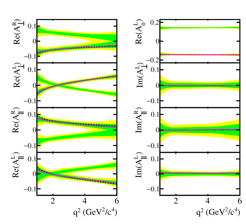
Figure 5: Distributions of the $\kern 1.61993pt\overline{\kern-1.61993ptB}{}^{0}$ amplitudes as a function of $q^{2}$ resulting from $10^{4}$ fits to generated signal and background simulated data under Scenario-II. The green and yellow bands correspond to the 68% and 95% confidence intervals respectively. The dotted line denotes the SM prediction as given by the EOS program [3]. The magenta solid line denotes the most likely value resulting from the ensemble of fits. A discrete symmetry of reflections about zero is observed due to the fact that the $J_{i}$ terms are bilinear coefficients of the amplitudes.

The complete set of $C\!P$-symmetric and $C\!P$-asymmetric observables, defined in Sec. 2, can be constructed out the $\kern 1.79993pt\overline{\kern-1.79993ptB}{}^{0}$ and $B^{0}$ amplitudes. A subset of these observables are shown in Figs. 6 and 7, for Scenario-II and Scenario-I respectively. The 68% and 95% bands are given as in Fig. 5.

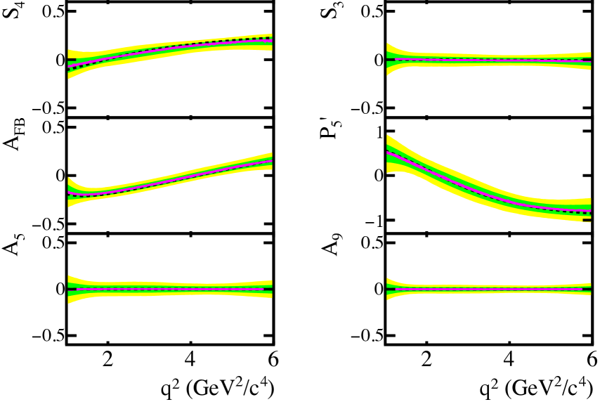
Figure 6: Subset of observables constructed out of the helicity-amplitudes, resulting from fits to ensembles of simulated data, under Scenario-II. The meaning of the various bands and curves is given in Fig 5.

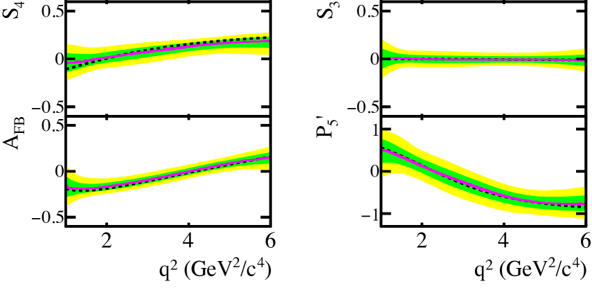
Figure 7: Subset of observables constructed out of the helicity-amplitudes, resulting from fits to ensembles of simulated data, under Scenario-I. The meaning of the various bands and curves is given in Fig 5.

In a minor part of the $q^{2}$ range, a bias at the level of $0.5\sigma$ is apparent in some observables, most notably $S_{4}$. The $S_{4}$ observable is sensitive to the interference between the $A_{\parallel}^{L}$ and $A_{0}^{L}$ amplitudes which in the fixed-basis is given by $\mathrm{Re}(A_{\parallel}^{L}A_{0}^{L})$. This bias arises from the approximate discrete symmetry discussed in Sec. 3.3. This accidental symmetry is more prone to occur in models where the right-handed Wilson Coefficients are zero, such as the SM. As this is an effect of the angular distribution, this type of bias would have to be taken into account for any fitting method employed, whether binned or unbinned in $q^{2}$.

4.1 Uncertainty estimation

The probability distribution function of the signal decay remains positive definite for all values of the amplitude coefficients. This fact, coupled with the expected LHCb sample sizes for Scenarios-I and II, means that the likelihood surface, constructed out of the data and the probability distributions of the signal and the background, should be a good estimator of the statistical uncertainty of the amplitude coefficients.

Table 3 summarises the pull mean and width of the amplitudes in the fixed-basis for Scenario-I at a point in $q^{2}$. In order to discern any statistical bias from the bias originating from the approximate symmetries discussed in Sec. 3.3, a point in $q^{2}$ is chosen such that minimises the bias from the approximate symmetries.

The pull means and widths are largely consistent with zero and unity, respectively, indicating that the likelihood is a good estimator of the uncertainty of the amplitudes. The residual bias in $A_{\parallel}^{R}$ arises from the additional approximate symmetry between $A_{\parallel}^{R}$ and $A_{\perp}^{R}$ discussed in Sec. 3.3. Figure 5 shows that there is no point in $q^{2}$ where the bias from the approximate symmetry can be removed for all the amplitudes simultaneously.

Table 3: Means and widths of the pull distributions of the P-wave amplitudes at $q^{2}=2.4$ ${\mathrm{\,Ge\kern-0.90005ptV^{2}\!/}c^{4}}$, obtained from fits to ensembles of simulated data samples in Scenario-I. The pull is defined as (Fit-SM)/$\sigma_{\mathrm{Meas.}}$ where $\sigma_{\mathrm{Meas.}}$ is the error on the measured quantity obtained using the error matrix of the fit. The deviation of the pull mean of $\mathrm{Re}(A_{\parallel}^{R})$ from zero arises due to the residual bias from the approximate symmetry of the angular distribution.

Parameter	Pull mean	Pull width
$\mathrm{Re}(A_{0}^{L})\kern 1.79993pt\overline{\kern-1.79993ptB}{}^{0}$	$-0.03\pm 0.02$	$0.97\pm 0.03$
$\mathrm{Re}(A_{\parallel}^{L})\kern 1.79993pt\overline{\kern-1.79993ptB}{}^{0}$	$\phantom{-}0.00\pm 0.02$	$1.01\pm 0.03$
$\mathrm{Im}(A_{\parallel}^{L})\kern 1.79993pt\overline{\kern-1.79993ptB}{}^{0}$	$\phantom{-}0.01\pm 0.02$	$1.02\pm 0.03$
$\mathrm{Re}(A_{\parallel}^{R})\kern 1.79993pt\overline{\kern-1.79993ptB}{}^{0}$	$\phantom{-}0.22\pm 0.02$	$0.90\pm 0.03$
$\mathrm{Im}(A_{\parallel}^{R})\kern 1.79993pt\overline{\kern-1.79993ptB}{}^{0}$	$-0.02\pm 0.02$	$0.94\pm 0.03$
$\mathrm{Re}(A_{\perp}^{L})\kern 1.79993pt\overline{\kern-1.79993ptB}{}^{0}$	$\phantom{-}0.02\pm 0.02$	$0.97\pm 0.03$
$\mathrm{Im}(A_{\perp}^{L})\kern 1.79993pt\overline{\kern-1.79993ptB}{}^{0}$	$-0.04\pm 0.02$	$0.95\pm 0.03$
$\mathrm{Re}(A_{\perp}^{R})\kern 1.79993pt\overline{\kern-1.79993ptB}{}^{0}$	$-0.05\pm 0.02$	$0.94\pm 0.03$

A subset of two dimensional profile-likelihood distributions is shown in Fig. 8. The profile likelihood is obtained by scanning over the two parameters in question, and minimising the likelihood over the rest of the parameters at each point. These profile likelihoods can be used to determine the confidence regions of the amplitude coefficients and therefore of the observables. The error matrix of the fit is a good approximation to the likelihood surface at the level of around $15\%$.

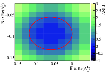
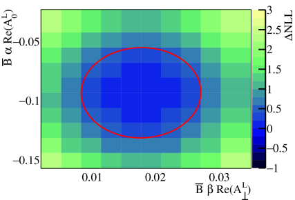
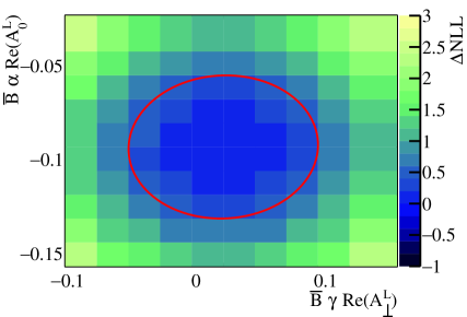
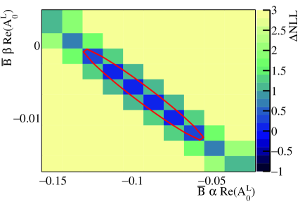
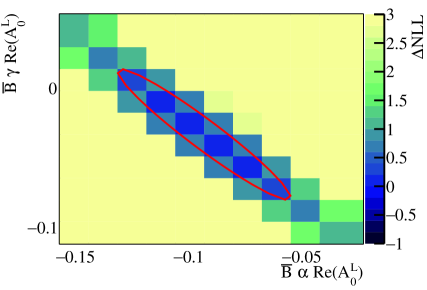
Figure 8: Subset of two dimensional profile likelihood distributions from a fit to a single simulated dataset in Scenario-I. The red ellipses denote the error and the correlation obtained from the error matrix of the fit.

For a given dataset, a prediction of the spin-amplitudes as a function of $q^{2}$ can be obtained for a particular value of the Wilson Coefficients and $B\rightarrow K^{*}$ form factors. In turn, each amplitude can be expressed in terms of the three parameter ansatz of Eq. (16), by transforming to the fixed-basis, using the procedure detailed in Appendix A. By fitting each transformed amplitude with the ansatz of Eq. (16), the coefficients $\alpha$, $\beta$ and $\gamma$ can be determined. The best fit point and the error matrix of the fit to the data, can then be used to place constraints on the Wilson Coefficients using a procedure like that employed in Refs. [17, 18, 19, 6, 22].

5 Sensitivity to new physics

The expected sensitivity to the effects of new physics (NP), neglecting theory uncertainties, is estimated by generating a large number of simulated data samples according to the SM (null dataset) and a NP model where $\delta C_{9}=-1.5$ (test dataset). The choice of the NP model is motivated by recent results from global fits to $b\rightarrow s\ell\ell$ and $b\rightarrow s\gamma$ measurements [17, 18, 19, 20, 21, 22, 23, 24, 25, 26, 27, 6, 28] which are dominated by LHCb’s anomalous results in the angular distribution of $\kern 1.79993pt\overline{\kern-1.79993ptB}{}^{0}\!\rightarrow\kern 1.99997pt\overline{\kern-1.99997ptK}{}^{*0}\mu^{+}\mu^{-}$ decays [15, 16]. The EOS program [3] is used to generate simulated data from these two models using their central value predictions. Two fits are then performed to an ensemble of simulated datasets generated with the SM and the NP model. In the first fit, the amplitude parameters are fixed to their SM values (null hypothesis). In the second fit, the amplitude parameters are fixed to the values given by the model with $\delta C_{9}=-1.5$ (test hypothesis). The background components and yields are treated as nuisance parameters and are left floating in each fit. The S-wave contribution in the $K\pi$ system of $\kern 1.79993pt\overline{\kern-1.79993ptB}{}^{0}\!\rightarrow\kern 1.99997pt\overline{\kern-1.99997ptK}{}^{*0}\mu^{+}\mu^{-}$ decays is less understood theoretically than the dominant P-wave part. In order to correctly model the S-wave component of the $K\pi$ system, experimental input is required. Therefore, for these sensitivity studies, the S-wave amplitudes are treated as nuisance parameters in the fit.

The test statistics are defined as

$$Q^{SM} =2(\mathrm{NLL}^{SM}_{{test}}-\mathrm{NLL}^{SM}_{{null}})$$

$$Q^{NP} =2(\mathrm{NLL}^{NP}_{{test}}-\mathrm{NLL}^{NP}_{{null}}),$$ (21)

where $\mathrm{NLL}^{SM,NP}_{{null,test}}$ corresponds to the negative log likelihood value of the null or test hypothesis on a SM or NP simulated dataset. The expected sensitivity to a model with $\delta C_{9}=-1.5$ is then estimated by counting the fraction of the toy simulations with a value of $Q^{SM}\leq\bar{Q}^{NP}$, where $\bar{Q}^{NP}$ is the median of the $Q^{NP}$ distribution. Figure 9 shows the distribution of the test statistic for both the SM and NP simulated data samples in fits to $B^{0}$ and $\kern 1.79993pt\overline{\kern-1.79993ptB}{}^{0}$ candidates separately, using a sample size equivalent to that expected at LHCb during Run-I of the LHC. The probability for the SM sample to fluctuate such that it gives a test statistic as low or lower than the median of the NP sample (i.e $Q^{SM}\leq\bar{Q}^{NP}$) corresponds to a significance of $6.5\sigma$. This significance is obtained for an idealised model of the experimental data and does not account for the theoretical uncertainties associated with the translation from Wilson coefficients to amplitudes.

For comparison with methods used previously, the same procedure for estimating the expected significance can be performed for fits directly to the $C\!P$-averaged observables, $S_{i}$ in bins of $q^{2}$. For these fits, three $q^{2}$ bins between $1<q^{2}<6$ ${\mathrm{\,Ge\kern-1.00006ptV^{2}\!/}c^{4}}$ are chosen as $(1,2.7)$, $(2.7,4.3)$, $(4.3,6)$ ${\mathrm{\,Ge\kern-1.00006ptV^{2}\!/}c^{4}}$. In this binned approach a combined significance of $5.0\sigma$ is obtained. Therefore, fitting for the $q^{2}$ dependent $K^{*0}$ spin-amplitudes, separately for the $B^{0}$ and the $\kern 1.79993pt\overline{\kern-1.79993ptB}{}^{0}$, results in a 30% improvement in the expected sensitivity. Equivalently, to get the same sensitivity as the amplitude method, a binned fit to the $C\!P$-averaged observables would require an additional 70% of integrated luminosity.

The inclusion of the $K\pi$ system in an S-wave configuration introduces six additional observables, as shown in Eq. (5), in contrast to four additional S-wave amplitude components. Approximately half of the increase in sensitivity detailed above, can be attributed to the reduced number of S-wave-related nuisance parameters present in the amplitude fits, and the other half owes to the intrinsic sensitivity of the method.

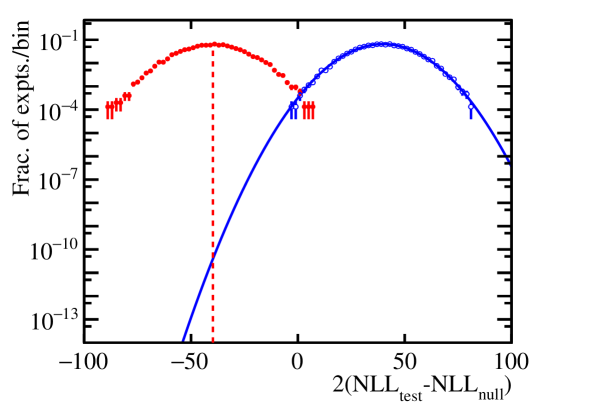
Figure 9: Distribution of the test statistic $Q^{NP,SM}$, for fits to the NP (red full points) and SM (blue open points) simulated data samples. The S-wave components are treated as nuisance parameters and are therefore floating in the fit. The dashed red line denotes the median of the test statistic from fits to the NP sample. The solid blue curve is a fit of a Gaussian distribution to the distribution of the test statistic from fits to the SM sample.

6 Conclusions

In summary, a method of analysing $\kern 1.79993pt\overline{\kern-1.79993ptB}{}^{0}\!\rightarrow\kern 1.99997pt\overline{\kern-1.99997ptK}{}^{*0}\mu^{+}\mu^{-}$ decays is presented that allows the determination of all of the $K^{*0}$ amplitudes as a parametric function of $q^{2}$. The method is applicable with the data sample that is already available at the LHCb experiment and works in the region where the amplitudes can be described by a simple functional form, $1<q^{2}<6$ ${\mathrm{\,Ge\kern-1.00006ptV^{2}\!/}c^{4}}$. The bias coming from the choice of $q^{2}$ parameterisation is much smaller than the statistical uncertainty of current and any forseeable-future experimental measurements.

The method overcomes several shortcomings of previous methods: As all the $\kern 1.99997pt\overline{\kern-1.99997ptK}{}^{*0}$ helicity amplitudes are determined from a single fit to data, the full correlations between experimentally determined quantities can be obtained, improving the sensitivity to new physics; fitting for the amplitudes enables all of the symmetries of the angular distribution for a $K\pi$ system in a P- and S-wave state to be accounted for, giving increased experimental precision compared to previous approaches which retain redundant degrees of freedom; the method avoids the integration of theoretical predictions over experimental $q^{2}$ bins, enabling the full exploitation of the cancellation of the form factors at leading order and therefore further improving the sensitivity to new physics.

The continuous symmetry transformations that can be applied to the amplitudes enable a modified basis to be specified, in which a number of amplitude components are set to zero. The basis considered by previous studies [11] gave a discontinuous shape in $q^{2}$, rendering the region $q^{2}<2.5$ ${\mathrm{\,Ge\kern-1.00006ptV^{2}\!/}c^{4}}$ unusable. Here, a new choice of basis is presented, which leaves the amplitudes smoothly varying in the entire range $1<q^{2}<6$ ${\mathrm{\,Ge\kern-1.00006ptV^{2}\!/}c^{4}}$ for the SM and for a wide range of new physics models. The present analysis also highlights new approximate discrete symmetries that are manifest for data samples on the order of that collected at LHCb during Run-I. These approximate symmetries are more prone to occur in models like the SM, where there are no right-handed currents.

In order to illustrate the options that are available to fit a given dataset, the sensitivity of the method is presented in two different scenarios. For a sample equivalent to the LHCb Run-I dataset, a model-dependent assumption is made that the only weak phases present in the amplitudes come from the CKM matrix elements. Given diagrams with non-zero weak phases are Cabibbo suppressed, this assumption results in $B^{0}$ and $\kern 1.79993pt\overline{\kern-1.79993ptB}{}^{0}$ amplitudes which are identical. The $C\!P$-averaged observables can then be determined with greater precision than would be possible if instead both the $C\!P$-averaged and $C\!P$-asymmetric observables were determined. For a sample equivalent to the LHCb Run-II dataset, the results are determined without this assumption and the sensitivity to both $C\!P$-averaged and $C\!P$-asymmetric observables is presented.

The recent anomalous result in the angular distribution of $\kern 1.79993pt\overline{\kern-1.79993ptB}{}^{0}\!\rightarrow\kern 1.99997pt\overline{\kern-1.99997ptK}{}^{*0}\mu^{+}\mu^{-}$ motivates the consideration of a new physics scenario with $\delta C_{9}=-1.5$ [15]. In such a scenario, the new method presented is 30% more sensitive than a three $q^{2}$-bin fit to the $C\!P$-averaged, $S_{i}$, in the region $1<q^{2}<6$ ${\mathrm{\,Ge\kern-1.00006ptV^{2}\!/}c^{4}}$, improving the discrimination between this scenario and the SM from 5.0 to 6.5 $\sigma$. An additional $\sim$70% of integrated luminosity would therefore be required in order for a fit to the $C\!P$-averaged observables to achieve the same sensitivity as the fit to the $\kern 1.99997pt\overline{\kern-1.99997ptK}{}^{*0}$ spin-amplitudes. This improvement arises from the treatment of the $q^{2}$ dependence of the amplitudes as a continuous function, and the use of all symmetry relations of the angular distribution to reduce the number of independent parameters that describe the $\kern 1.79993pt\overline{\kern-1.79993ptB}{}^{0}\!\rightarrow\kern 1.99997pt\overline{\kern-1.99997ptK}{}^{*0}\mu^{+}\mu^{-}$ decay.

Appendix A Amplitude transformation and parametrisation

The spin-amplitudes in the fixed-basis can be determined by applying Eq. (10) to a set of amplitudes in the original basis. The transformation angles, $\phi_{L},\phi_{R},\theta,\omega$ can be determined in terms of the original amplitudes, by requiring that in the fixed-basis Eq. (13) holds, and solving a system of four non-linear equations. The analytical expressions of the transformation angles are given in Ref. [36] and shown below

$$\tan{2\omega} =2\frac{\mathrm{Im}(A_{0}^{R})\mathrm{Re}(A_{0}^{L})+(L\leftrightarrow R)}{|A_{0}^{R}|^{2}-|A_{0}^{L}|^{2}}$$

$$\tan\theta =\frac{\mathrm{Re}(A_{0}^{R})+\mathrm{Im}(A_{0}^{L})\tan\omega}{-\mathrm{Re}(A_{0}^{L})+\mathrm{Im}(A_{0}^{R})\tan\omega}$$

$$\tan\phi_{L} =\frac{\mathrm{Im}(A_{0}^{L})+\mathrm{Im}A_{0}^{R}\tan\theta-[\mathrm{Re}(A_{0}^{R})-\mathrm{Re}(A_{0}^{L})\tan\theta]\tan\omega}{-\mathrm{Re}(A_{0}^{L})+\mathrm{Re}(A_{0}^{R})\tan\theta+[\mathrm{Im}(A_{0}^{R})+\mathrm{Im}(A_{0}^{L})\tan\theta]\tan\omega}$$

$$\tan\phi_{R} =\frac{\mathrm{Im}(A_{\perp}^{R})+\mathrm{Im}(A_{\perp}^{L})\tan\theta-[\mathrm{Re}(A_{\perp}^{L})-\mathrm{Re}(A_{\perp}^{R})\tan\theta]\tan\omega}{-\mathrm{Re}(A_{\perp}^{R})+\mathrm{Re}(A_{\perp}^{L})\tan\theta+[\mathrm{Im}(A_{\perp}^{L})+\mathrm{Im}(A_{\perp}^{R})\tan\theta]\tan\omega},$$

where $A_{i}^{L,R}$ are the $\kern 1.99997pt\overline{\kern-1.99997ptK}{}^{*0}$ amplitudes in the original basis.

A C++ library will be provided shortly, which will transform a given set of amplitudes to the fixed-basis, and perform a fit in $q^{2}$ to determine the coefficients $\alpha,~{}\beta,~{}\gamma$ of the $q^{2}$ ansatz of Eq. (16). In addition, provided there is a consensus in the experimental community, the likelihood function of Eq. (19) could be made publicly available, along with tools that minimise the likelihood over the nuisance parameters, for a given set of amplitudes.

References

- [1] W. Altmannshofer et al., Symmetries and asymmetries of decays in the Standard Model and beyond, JHEP 01 (2009) 019, arXiv:0811.1214
- [2] C. Bobeth, G. Hiller, and G. Piranishvili, CP asymmetries in and untagged , decays at NLO, JHEP 07 (2008) 106, arXiv:0805.2525
- [3] C. Bobeth, G. Hiller, and D. van Dyk, The benefits of decays at low recoil, JHEP 07 (2010) 098, arXiv:1006.5013
- [4] D. Das and R. Sinha, New physics effects and hadronic form factor uncertainties in , Phys. Rev. D86 (2012) 056006, arXiv:1205.1438
- [5] R. R. Horgan, Z. Liu, S. Meinel, and M. Wingate, Calculation of and observables using form factors from lattice QCD, Phys. Rev. Lett. 112 (2014) 212003, arXiv:1310.3887
- [6] F. Mahmoudi, S. Neshatpour, and J. Virto, optimised observables in the MSSM, Eur. Phys. J. C74 (2014) 2927, arXiv:1401.2145
- [7] C. Hambrock, G. Hiller, S. Schacht, and R. Zwicky, form factors from flavor data to QCD and back, Phys. Rev. D89 (2014) 074014, arXiv:1308.4379
- [8] T. Hurth, F. Mahmoudi, and S. Neshatpour, Global fits to b data and signs for lepton non-universality, JHEP 12 (2014) 053, arXiv:1410.4545
- [9] F. Kruger, L. M. Sehgal, N. Sinha, and R. Sinha, Angular distribution and CP asymmetries in the decays and , Phys. Rev. D61 (2000) 114028, Erratum ibid. D63 (2001) 019901, arXiv:hep-ph/9907386
- [10] F. Kruger and J. Matias, Probing new physics via the transverse amplitudes of at large recoil, Phys. Rev. D71 (2005) 094009, arXiv:hep-ph/0502060
- [11] U. Egede et al., On the new physics reach of the decay mode , JHEP 10 (2010) 056, arXiv:1005.0571
- [12] C. Bobeth, G. Hiller, and D. van Dyk, More benefits of semileptonic rare decays at low recoil: Violation, JHEP 07 (2011) 067, arXiv:1105.0376
- [13] S. Descotes-Genon, J. Matias, M. Ramon, and J. Virto, Implications from clean observables for the binned analysis of at large recoil, JHEP 01 (2013) 048, arXiv:1207.2753
- [14] S. Descotes-Genon, T. Hurth, J. Matias, and J. Virto, Optimizing the basis of observables in the full kinematic range, JHEP 05 (2013) 137, arXiv:1303.5794
- [15] LHCb collaboration, R. Aaij et al., Measurement of form-factor-independent observables in the decay , Phys. Rev. Lett. 111 (2013) 191801, arXiv:1308.1707
- [16] LHCb collaboration, Angular analysis of the decay, LHCb-CONF-2015-002
- [17] S. Descotes-Genon, J. Matias, and J. Virto, Understanding the Anomaly, Phys. Rev. D88 (2013) 074002, arXiv:1307.5683
- [18] W. Altmannshofer and D. M. Straub, New physics in ?, Eur. Phys. J. C73 (2013) 2646, arXiv:1308.1501
- [19] F. Beaujean, C. Bobeth, and D. van Dyk, Comprehensive Bayesian analysis of rare (semi)leptonic and radiative decays, Eur. Phys. J. C74 (2014) 2897, arXiv:1310.2478
- [20] T. Hurth and F. Mahmoudi, On the LHCb anomaly in B , JHEP 04 (2014) 097, arXiv:1312.5267
- [21] S. Jäger and J. Martin Camalich, On at small dilepton invariant mass, power corrections, and new physics, JHEP 05 (2013) 043, arXiv:1212.2263
- [22] S. Jäger and J. Martin Camalich, Reassessing the discovery potential of the decays in the large-recoil region: SM challenges and BSM opportunities, arXiv:1412.3183
- [23] S. Descotes-Genon, L. Hofer, J. Matias, and J. Virto, On the impact of power corrections in the prediction of observables, JHEP 12 (2014) 125, arXiv:1407.8526
- [24] W. Altmannshofer, S. Gori, M. Pospelov, and I. Yavin, Quark flavor transitions in models, Phys. Rev. D89 (2014) 095033, arXiv:1403.1269
- [25] A. Crivellin, G. D’Ambrosio, and J. Heeck, Explaining , and in a two-Higgs-doublet model with gauged , arXiv:1501.00993
- [26] R. Gauld, F. Goertz, and U. Haisch, An explicit Z’-boson explanation of the anomaly, JHEP 01 (2014) 069, arXiv:1310.1082
- [27] W. Altmannshofer and D. M. Straub, State of new physics in transitions, arXiv:1411.3161
- [28] A. Datta, M. Duraisamy, and D. Ghosh, Explaining the data with scalar interactions, Phys. Rev. D89 (2014) 071501, arXiv:1310.1937
- [29] S. D. Aristizabal, F. Staub, and A. Vicente, Shedding light on the anomalies with a dark sector, arXiv:1503.06077
- [30] J. Lyon and R. Zwicky, Resonances gone topsy turvy - the charm of QCD or new physics in ?, arXiv:1406.0566
- [31] A. Khodjamirian, T. Mannel, and Y. M. Wang, decay at large hadronic recoil, JHEP 02 (2013) 010, arXiv:1211.0234
- [32] A. Khodjamirian, T. Mannel, A. A. Pivovarov, and Y.-M. Wang, Charm-loop effect in and , JHEP 09 (2010) 89, arXiv:1006.4945
- [33] LHCb collaboration, R. Aaij et al., Differential branching fraction and angular analysis of the decay , JHEP 08 (2013) 131, arXiv:1304.6325
- [34] J. Matias, F. Mescia, M. Ramon, and J. Virto, Complete anatomy of and its angular distribution, JHEP 04 (2012) 104, arXiv:1202.4266
- [35] T. Blake, U. Egede, and A. Shires, The effect of S-wave interference on the angular observables, JHEP 03 (2013) 027, arXiv:1210.5279
- [36] L. Hofer and J. Matias, Exploiting the symmetries of P and S-wave for , arXiv:1502.00920
- [37] D. Becirevic and A. Tayduganov, Impact on the new physics search in decay, Nuclear Physics B868 (2013) 368 , arXiv:1207.4004
- [38] D. Das, G. Hiller, M. Jung, and A. Shires, The and distributions at low hadronic recoil, JHEP 09 (2014) 109, arXiv:1406.6681
- [39] C.-D. Lü and W. Wang, Analysis of in the higher kaon resonance region, Phys. Rev. D 85 (2012) 034014, arXiv:1111.1513
- [40] Particle Data Group, J. Beringer et al., Review of particle physics, Phys. Rev. D86 (2012) 010001
- [41] U.-G. Meisner and W. Wang, Generalized heavy-to-light form factors in light-cone sum rules, Physics Letters B730 (2014) 336 , arXiv:1312.3087